
A New Concept of Soil Line Retrieval from Landsat 8 Images for Estimating Plant Biophysical Parameters


Abstract
:
1. Introduction
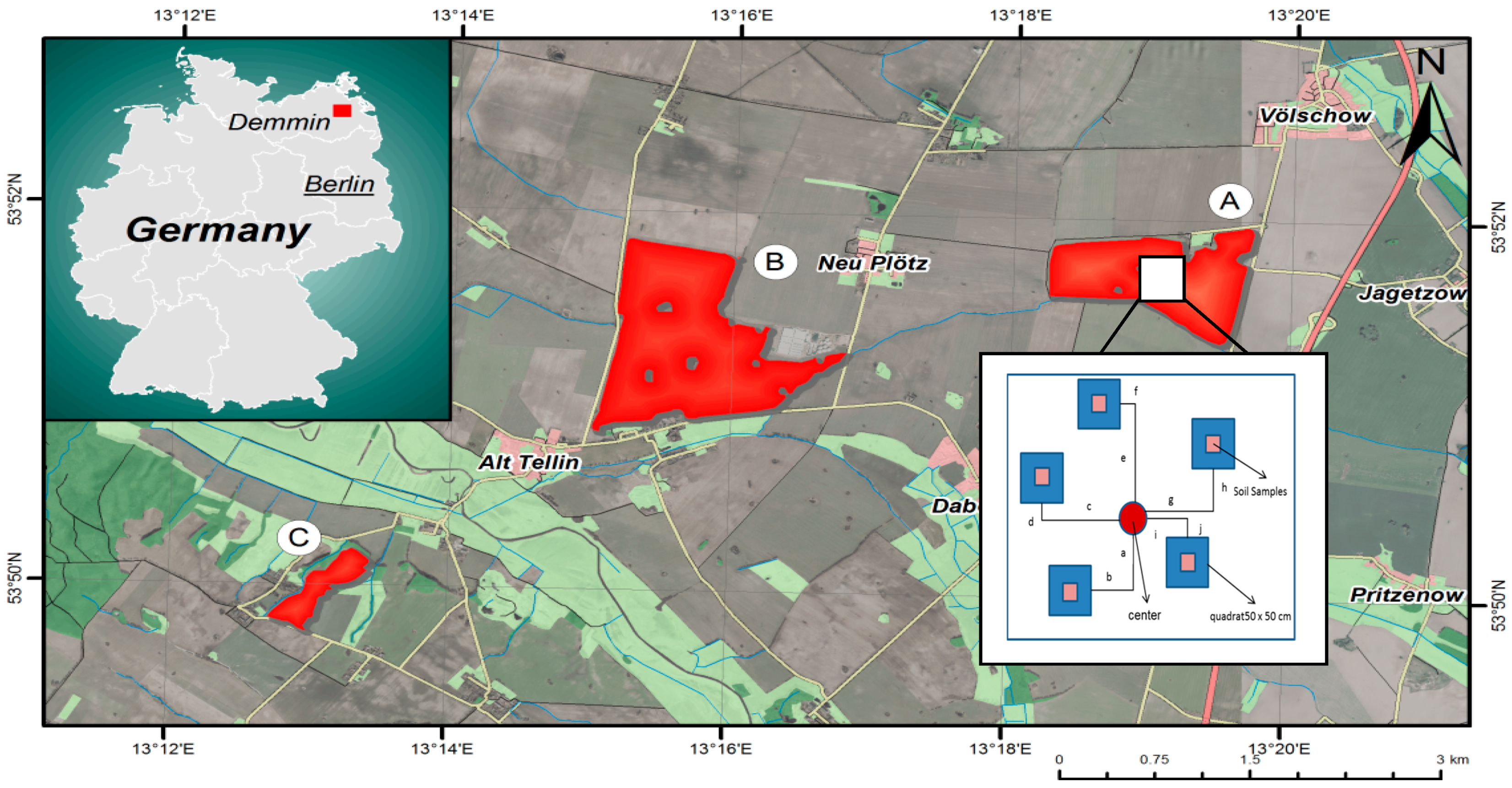
2. Test Site and Study Area
3. Materials
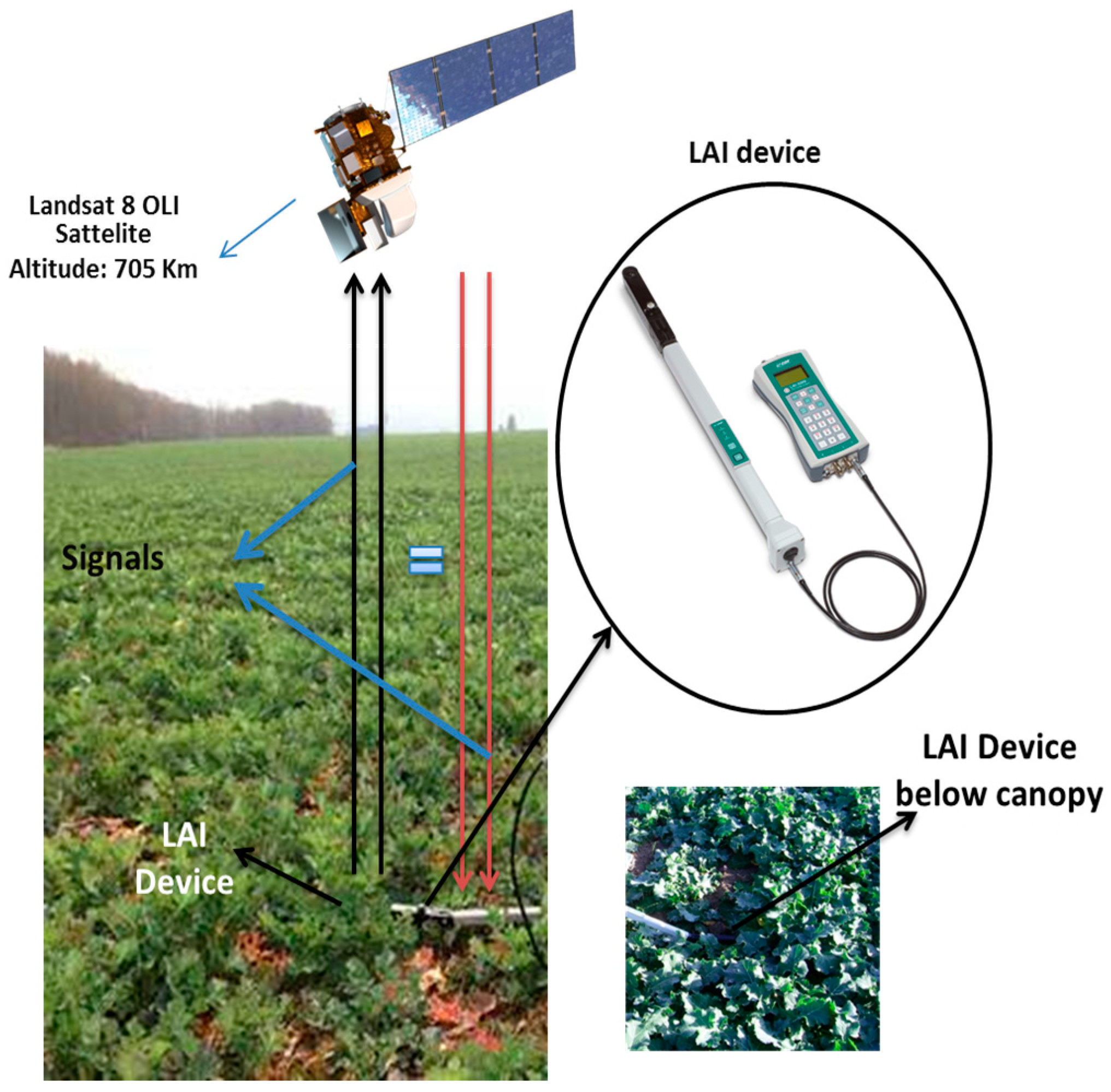
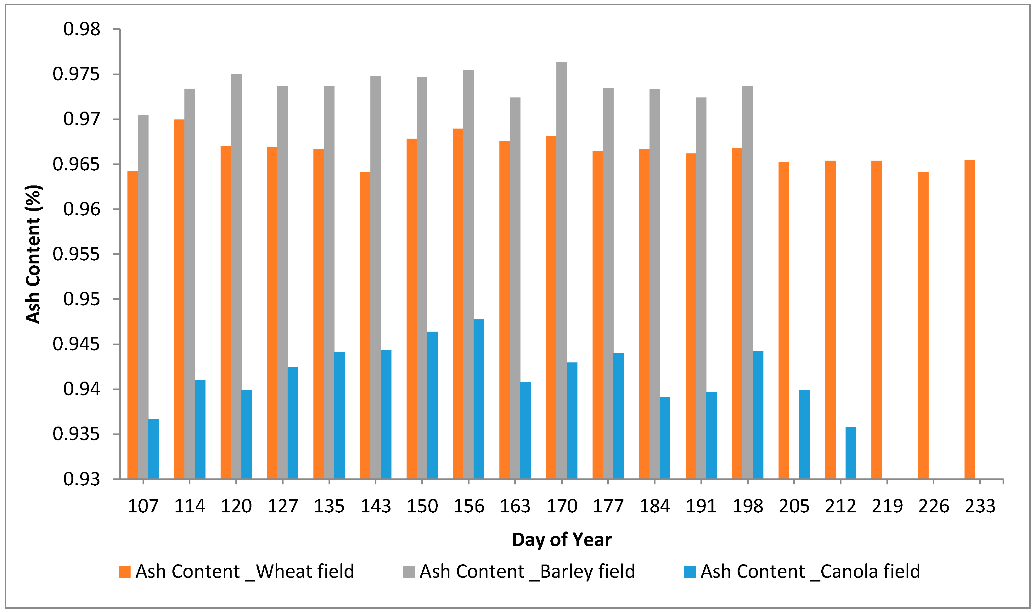
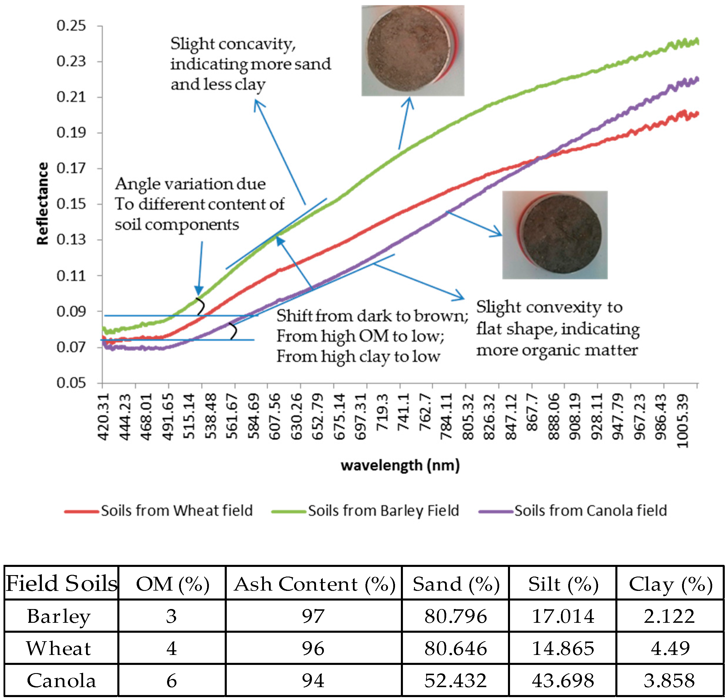
3.1. Field Data and Laboratory Analysis
3.2. Satellite Data
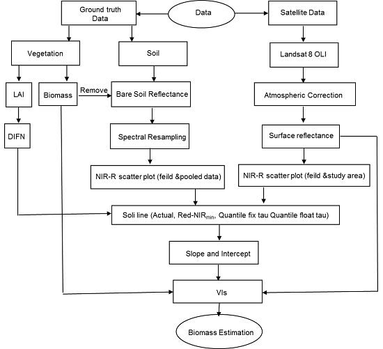
4. Methods
4.1. (Red-NIRmin) Regression Method
4.2. Quantile Regression Method
4.3. SL-Related Vegetation Indices and Validation
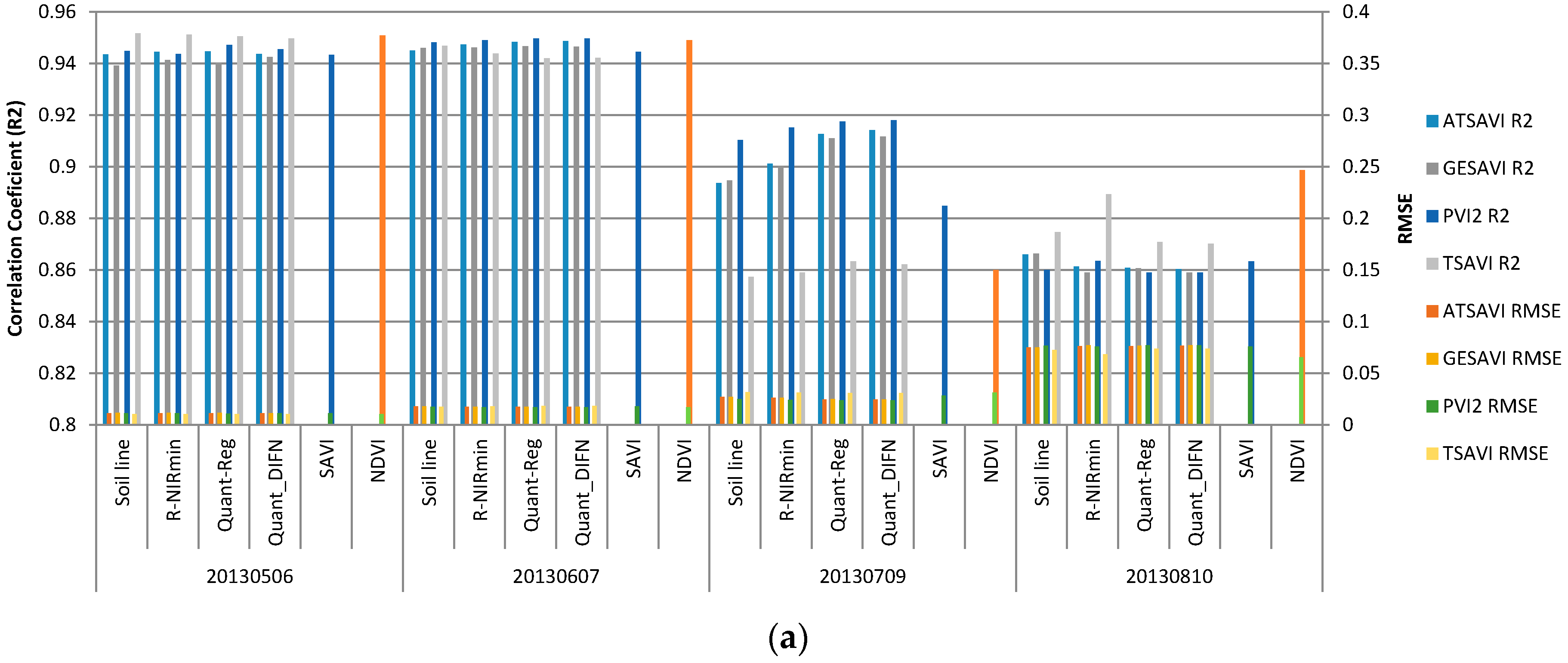
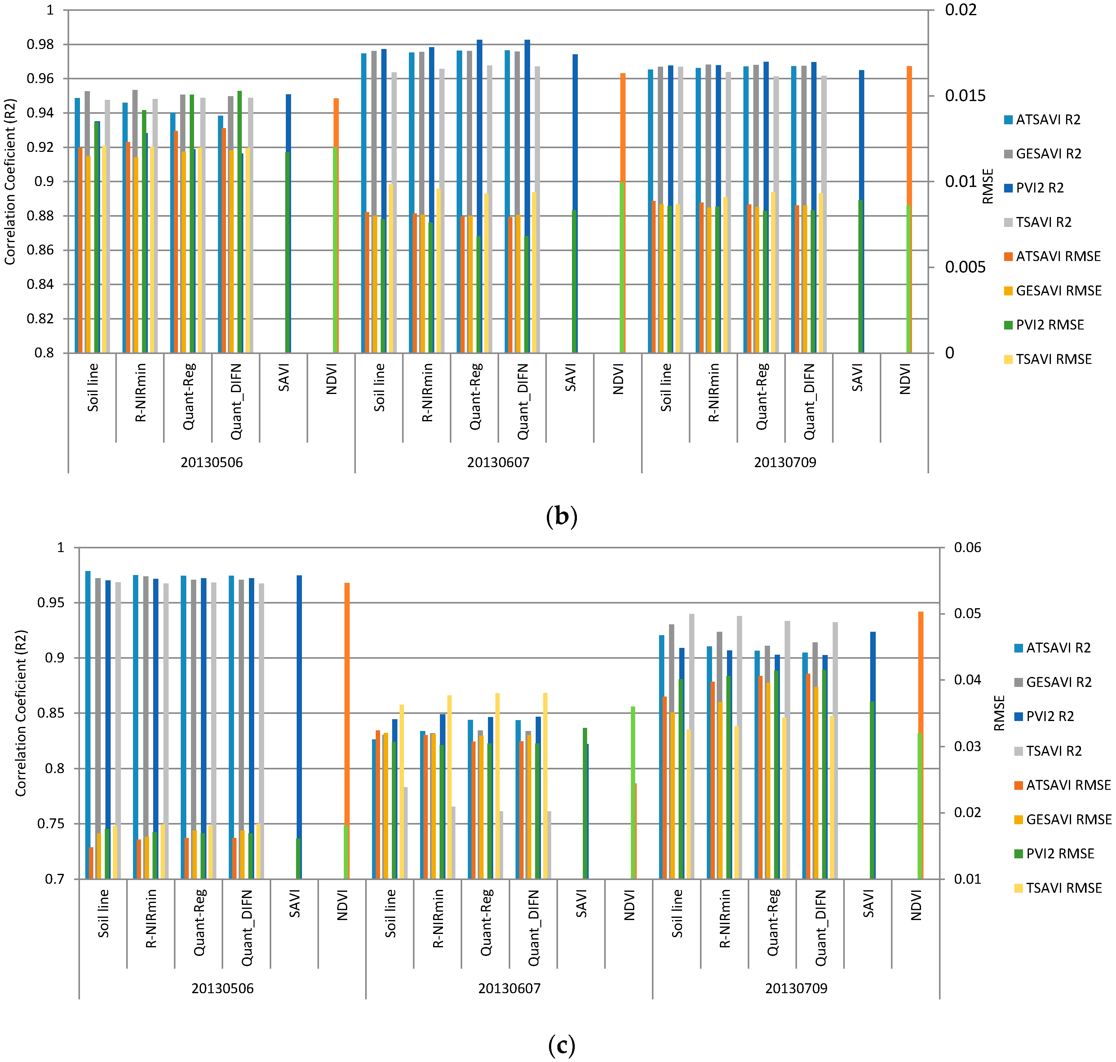
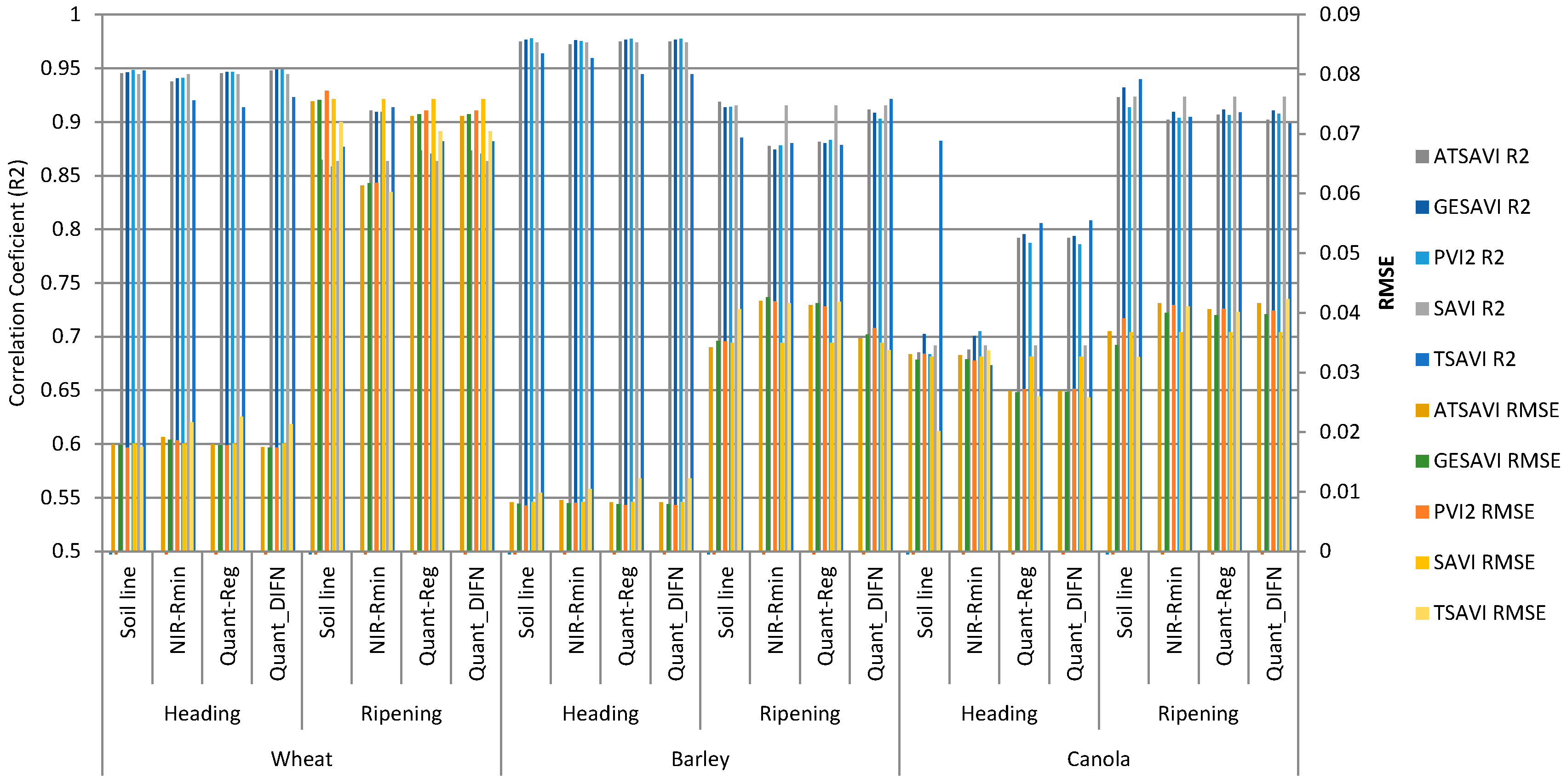
5. Results
6. Discussion
7. Conclusions
Acknowledgments
Author Contributions
Conflicts of Interest
References
- Baret, F.; Jacquemoud, S.; Hanocq, J.F. The soil line concept in remote sensing. Remote Sens. Rev. 1993, 7, 65–82. [Google Scholar] [CrossRef]
- Nanni, M.R.; Demattê, J.A.M. Comportamento da linha do solo obtida por espectrorradiometria laboratorial para diferentes classes de solo. Rev. Bras. Ciência Solo 2006, 30, 1031–1038. [Google Scholar] [CrossRef]
- Jasinski, M.F.; Eagleson, P.S. The structure of red-infrared scattergrams of semivegetated landscapes. IEEE Trans. Geosci. Remote Sens. 1989, 27, 441–451. [Google Scholar] [CrossRef]
- Chang, C.-W.; Laird, D.A.; Mausbach, M.J.; Hurburgh, C.R. Near-infrared reflectance spectroscopy—Principal components regression analyses of soil properties. Soil Sci. Soc. Am. J. 2001, 65, 480–490. [Google Scholar] [CrossRef]
- Cierniewski, J. A model for soil surface roughness influence on the spectral response of bare soils in the visible and near-infrared range. Remote Sens. Environ. 1987, 23, 97–115. [Google Scholar] [CrossRef]
- Rondeaux, G.; Steven, M.; Baret, F. Optimization of soil-adjusted vegetation indices. Remote Sens. Environ. 1996, 55, 95–107. [Google Scholar] [CrossRef]
- Demattê, J.A.; Campos, R.C.; Cardoso Alves, M.; Fiorio, P.R.; Nanni, M.R. Visible–NIR reflectance: A new approach on soil evaluation. Geoderma 2004, 121, 95–112. [Google Scholar] [CrossRef]
- Fox, G.A.; Sabbagh, G.J.; Searcy, S.W.; Yang, C. An automated soil line identification routine for remotely sensed images. Soil Sci. Soc. Am. J. 2004, 68, 1326–1331. [Google Scholar] [CrossRef]
- Kaleita, A.L.; Tian, L.F.; Hirschi, M.C. Relationship between soil moisture content and soil surface reflectance. Trans. ASAE 2005, 48, 1979–1986. [Google Scholar] [CrossRef]
- Bowers, S.A.; Hanks, R.J. Reflection of radiant energy from soils. TRID 1965, 100, 130–138. [Google Scholar] [CrossRef]
- Baumgardner, M.F.; Silva, L.F.; Biehl, L.L.; Stoner, E.R. Reflectance properties of soils. In Advances in Agronomy; Brady, N.C., Ed.; Academic Press: New York, NY, USA, 1985; Volume 38, pp. 2–44. [Google Scholar]
- Xu, D.; Guo, X. A Study of soil line simulation from Landsat images in mixed grassland. Remote Sens. 2013, 5, 4533–4550. [Google Scholar] [CrossRef]
- Kauth, R.J.; Thomas, G.S. The tasseled cap—A graphic description of the spectral-temporal development of agricultural crops as seen by Landsat. In Proceedings of the Symposium on Machine Processing of Remotely Sensed Data, West Lafayette, IN, USA, 29 June–1 July 1976; pp. 41–51.
- Jackson, R. Spectral indices in N-Space. Remote Sens. Environ. 1983, 13, 409–421. [Google Scholar] [CrossRef]
- Richardson, A.J.; Wiegand, C.L. Distinguishing vegetation from soil background information (by gray mapping of Landsat MSS data). Photogramm. Eng. Remote Sens. 1977, 43, 1541–1552. [Google Scholar]
- Baret, F.; Guyot, G. Potentials and limits of vegetation indices for LAI and APAR assessment. Remote Sens. Environ. 1991, 35, 161–173. [Google Scholar] [CrossRef]
- Broge, N.H.; Mortensen, J.V. Deriving green crop area index and canopy chlorophyll density of winter wheat from spectral reflectance data. Remote Sens. Environ. 2002, 81, 45–57. [Google Scholar] [CrossRef]
- Díaz, B.M.; Blackburn, G.A. Remote sensing of mangrove biophysical properties: Evidence from a laboratory simulation of the possible effects of background variation on spectral vegetation indices. Int. J. Remote Sens. 2003, 24, 53–73. [Google Scholar] [CrossRef]
- Baret, F.; Jacquemoud, S.; Hanocq, J.F. About the soil line concept in remote sensing. Adv. Space Res. 1993, 13, 281–284. [Google Scholar] [CrossRef]
- Huete, A.R. Soil influences in remotely sensed vegetation-canopy spectra. Theory Appl. Opt. Remote Sens. 1989, 107–141. [Google Scholar]
- Gitelson, A.A.; Stark, R.; Grits, U.; Rundquist, D.; Kaufman, Y.; Derry, D. Vegetation and soil lines in visible spectral space: A concept and technique for remote estimation of vegetation fraction. Int. J. Remote Sens. 2002, 23, 2537–2562. [Google Scholar] [CrossRef]
- Flénet, F.; Kiniry, J.R.; Board, J.E.; Westgate, M.E.; Reicosky, D.C. Row spacing effects on light extinction coefficients of corn, sorghum, soybean, and sunflower. Agron. J. 1996, 88, 185–190. [Google Scholar] [CrossRef]
- Jordan, C.F. Derivation of leaf-area index from quality of light on the forest floor. Ecology 1969, 50, 663–666. [Google Scholar] [CrossRef]
- Tucker, C.J. Red and photographic infrared linear combinations for monitoring vegetation. Remote Sens. Environ. 1979, 8, 127–150. [Google Scholar] [CrossRef]
- Thoma, D.P.; Gupta, S.C.; Bauer, M.E. Evaluation of optical remote sensing models for crop residue cover assessment. J. Soil Water Conserv. 2004, 59, 224–233. [Google Scholar]
- Zhao, D.; Yang, T.; An, S. Effects of crop residue cover resulting from tillage practices on LAI estimation of wheat canopies using remote sensing. Int. J. Appl. Earth Obs. Geoinf. 2012, 14, 169–177. [Google Scholar] [CrossRef]
- Locke, C.R.; Carbone, G.J.; Filippi, A.M.; Sadler, E.J.; Gerwig, B.K.; Evans, D.E. Using remote sensing and modeling to measure crop biophysical variability. In Proceedings of the 5th International Conference on Precision Agriculture, Madison, WI, USA, 16–19 July 2000.
- Fox, G.A.; Metla, R. Soil property analysis using principal components analysis, soil line, and regression models. Soil Sci. Soc. Am. J. 2005, 69, 1782–1788. [Google Scholar] [CrossRef]
- Amani, M.; Mobasheri, M.R. A parametric method for estimation of leaf area index using Landsat ETM+ data. GISci. Remote Sens. 2015, 52, 478–497. [Google Scholar] [CrossRef]
- Fox, G.A.; Sabbagh, G.J. Estimation of soil organic matter from red and near-infrared remotely sensed data using a soil line Euclidean distance technique. Soil Sci. Soc. Am. J. 2002, 66, 1922–1929. [Google Scholar] [CrossRef]
- Shrestha, D.P. Mapping salinity hazard. In Remote Sensing of Soil Salinization; Metternicht, G., Zinck, J.A., Eds.; CRC Press: Boca Raton, FL, USA, 2008; pp. 257–270. [Google Scholar]
- Gilabert, M.A.; González-Piqueras, J.; García-Haro, F.J.; Meliá, J. A generalized soil-adjusted vegetation index. Remote Sens. Environ. 2002, 82, 303–310. [Google Scholar] [CrossRef]
- Gerighausen, H.; Borg, E.; Wloczyk, C.; Fichtelmann, B.; Günther, A.; Vajen, H.-H.; Rosenberg, M.; Schulz, M.; Engler, H.-G. DEMMIN—A test site for the validation of Remote Sensing data products. General description and application during AgriSAR 2006. In Proceedings of the Final Workshop on AGRISAR and EAGLE Campaigns, Noordwijk, The Netherlands, 15–16 October 2007.
- DLR Earth Observation Center. Available online: http://www.dlr.de/eoc/en/desktopdefault.aspx/tabid-5395/10255_read-40097 (accessed on 29 August 2016).
- Kaufman, Y.J.; Wald, A.E.; Remer, L.A.; Flynn, L. The MODIS 2.1-μm channel-correlation with visible reflectance for use in remote sensing of aerosol. IEEE Trans. Geosci. Remote Sens. 1997, 35, 1286–1298. [Google Scholar] [CrossRef]
- Berk, A.; Bernstein, L.S.; Anderson, G.P.; Acharya, P.K.; Robertson, D.C.; Chetwynd, J.H.; Adler-Golden, S.M. MODTRAN cloud and multiple scattering upgrades with application to AVIRIS. Remote Sens. Environ. 1998, 65, 367–375. [Google Scholar] [CrossRef]
- Dantzig, G. Linear Programming and Extensions; Princeton University Press: Princeton, NJ, USA, 1963. [Google Scholar]
- Koenker, R.; Bassett, G. Regression quantiles. Econometrica 1978, 46, 33–50. [Google Scholar] [CrossRef]
- Koenker, R. Quantile Regression in R: A Vignette. Available online: http://www.econ.uiuc.edu/~roger/research/rq/vig.pdf/ (accessed on 31 August 2016).
- Tsionas, E.G. Bayesian quantile inference. J. Stat. Comput. Simul. 2003, 73, 659–674. [Google Scholar] [CrossRef]
- Young, T.M.; Shaffer, L.B.; Guess, F.M.; Bensmail, H.; León, R.V. A comparison of multiple linear regression and quantite regression for modeling the internal bond of medium density fiberboard. For. Prod. J. 2008, 58, 39–48. [Google Scholar]
- Cade, B.S.; Terrell, J.W.; Neely, B.C. Estimating geographic variation in allometric growth and body condition of blue suckers with quantile regression. Trans. Am. Fish. Soc. 2011, 140, 1657–1669. [Google Scholar] [CrossRef]
- Koenker, R.; Machado, J.A.F. Goodness of fit and related inference processes for quantile regression. J. Am. Stat. Assoc. 1999, 94, 1296–1310. [Google Scholar] [CrossRef]
- Mills, A.J.; Fey, M.V.; Gröngröft, A.; Petersen, A.; Medinski, T.V. Unravelling the effects of soil properties on water infiltration: Segmented quantile regression on a large data set from arid South-West Africa. Aust. J. Soil Res. 2006, 44, 783–797. [Google Scholar] [CrossRef]
- Mills, A.; Fey, M.; Donaldson, J.; Todd, S.; Theron, L. Soil infiltrability as a driver of plant cover and species richness in the semi-arid Karoo, South Africa. Plant Soil 2009, 320, 321–332. [Google Scholar] [CrossRef]
- Tivoli, B.; Calonnec, A.; Richard, B.; Ney, B.; Andrivon, D. Current knowledge on plant/canopy architectural traits that reduce the expression and development of epidemics. Eur. J. Plant Pathol. 2013, 135, 471–478. [Google Scholar] [CrossRef]
- Olson, B.E.; Wallander, R.T.; Beaver, J.M. Comparing nondestructive measures of forage structure and phytomass. Can. J. Plant Sci. 2000, 80, 565–573. [Google Scholar] [CrossRef]
- Mabhaudhi, T.; Modi, A.T. Growth, phenological and yield responses of a bambara groundnut (Vigna subterranea (L.) Verdc.) landrace to imposed water stress under field conditions. South Afr. J. Plant Soil 2013, 30, 69–79. [Google Scholar] [CrossRef]
- The Hydrological Open Air Laboratory. Available online: http://hoal.hydrology.at/ (accessed on 22 July 2016).
- LI-CORE. Available online: https://www.licor.com/env/products/leaf_area/LAI-2200/ (accessed on 29 August 2016).
- Baret, F.; Guyot, G.; Major, D.J. TSAVI: A vegetation index which minimizes soil brightness effects on LAI and APAR estimation. In Proceedings of the IEEE 12th Canadian Symposium on Remote Sensing, Vancouver, BC, Canada, 10–14 July 1989; pp. 1355–1358.
- Huete, A.R. A soil-adjusted vegetation index (SAVI). Remote Sens. Environ. 1988, 25, 295–309. [Google Scholar] [CrossRef]
- Rouse, J.W., Jr.; Haas, R.H.; Schell, J.A.; Deering, D.W. Monitoring vegetation systems in the Great Plains with ERTS. NASA Spececr. Publ. 1974, 351, 309. [Google Scholar]
- Olden, J.D.; Jackson, D.A. Torturing data for the sake of generality: How valid are our regression models? Ecoscience 2000, 7, 501–510. [Google Scholar]
- Automated Radiative Transfer Models Operator (ARTMO). Available online: http://ipl.uv.es/artmo/ (accessed on 29 August 2016).
- Dematte, J.A.M.; Huete, A.R.; Ferreira, L.G.; Nanni, M.R.; Alves, M.C.; Fiorio, P.R. Methodology for bare soil detection and discrimination by Landsat TM Image. Open Remote Sens. J. 2009, 2, 24–35. [Google Scholar] [CrossRef]
- Nanni, M.R.; Demattê, J.A.M. Spectral reflectance methodology in comparison to traditional soil analysis. Soil Sci. Soc. Am. J. 2006, 70, 393–407. [Google Scholar] [CrossRef]
- Torrion, J.; Maas, S.; Guo, W.; Bordovsky, J.; Cranmer, A. A three-dimensional index for characterizing crop water stress. Remote Sens. 2014, 6, 4025–4042. [Google Scholar] [CrossRef]
- Demattê, J.A.M.; Bellinaso, H.; Romero, D.J.; Fongaro, C.T. Morphological interpretation of reflectance spectrum (MIRS) using libraries looking towards soil classification. Sci. Agric. 2014, 71, 509–520. [Google Scholar] [CrossRef]
- Maas, S.J.; Rajan, N. Normalizing and converting image dc data using scatter plot matching. Remote Sens. 2010, 2, 1644–1661. [Google Scholar] [CrossRef]
- Huete, A.R.; Post, D.F.; Jackson, R.D. Soil spectral effects on 4-space vegetation discrimination. Remote Sens. Environ. 1984, 15, 155–165. [Google Scholar] [CrossRef]
- Huete, A.; Miura, T.; Yoshioka, H.; Ratana, P.; Broich, M. Indices of vegetation activity. In Biophysical Applications of Satellite Remote Sensing; Hanes, J.M., Ed.; Springer: Berlin/Heidelberg, Germany, 2014; pp. 1–41. [Google Scholar]
- Yoshioka, H.; Miura, T.; Demattê, J.A.M.; Batchily, K.; Huete, A.R. Derivation of soil line influence on two-band vegetation indices and vegetation isolines. Remote Sens. 2009, 1, 842–857. [Google Scholar] [CrossRef]
- Yoshioka, H.; Miura, T.; Demattê, J.A.M.; Batchily, K.; Huete, A.R. Soil line influences on two-band vegetation indices and vegetation isolines: A numerical study. Remote Sens. 2010, 2, 545–561. [Google Scholar] [CrossRef]
- Thompson, D.R.; Wehmanen, O.A. Using Landsat digital data to detect moisture stress in corn-soybean growing regions. Photogramm. Eng. Remote Sens. 1980, 45, 201–207. [Google Scholar]
- Galvão, L.S.; Vitorello, Í. Variability of laboratory measured soil lines of soils from southeastern Brazil. Remote Sens. Environ. 1998, 63, 166–181. [Google Scholar] [CrossRef]
- Elvidge, C.D.; Chen, Z. Comparison of broad-band and narrow-band red and near-infrared vegetation indices. Remote Sens. Environ. 1995, 54, 38–48. [Google Scholar] [CrossRef]
- Ahmadian, N.; Ghasemi, S.; Wigneron, J.-P.; Zölitz, R. Comprehensive study of the biophysical parameters of agricultural crops based on assessing Landsat 8 OLI and Landsat 7 ETM+ vegetation indices. GISci. Remote Sens. 2016, 53, 337–359. [Google Scholar] [CrossRef]


| Ground Truth Data Samples from Field Observation | Landsat 8 OLI Satellite Data 1 | ||||||
|---|---|---|---|---|---|---|---|
| Crop Type | Dry Biomass 2 | DIFN (LAI) 3 | Soil Samples (Ash Content) | Field Spectrometer 4 | Soil Granulometric Analysis 5 | Local | Field |
| Wheat | 190 | 228 | 95 | 88 | 10 | 4 (126, 158, 190, 222) | 2 (158, 222) |
| Barley | 140 | 168 | 70 | 80 | 10 | 3 (126, 158, 190) | 3 (158, 197, 238) |
| Canola | 160 | 192 | 80 | 79 | 10 | 3 (126, 158, 190) | 2 (165, 190) |
| Vegetation Index | Algorithm | Description |
|---|---|---|
| PVI [15] | a = slope of the SL, b = intercept of the SL | |
| TSAVI 2 or ATSAVI [16] | a = slope of the SL, b = intercept of the SL, X = 0.08 | |
| GESAVI [32] | Z = 0.35, b = slope of the SL, a = intercept of the SL | |
| TSAVI [51] | a = slope of the SL, b = intercept of the SL | |
| SAVI [52] | L = 0.5 (soil adjustment factor) | |
| NDVI [53] |
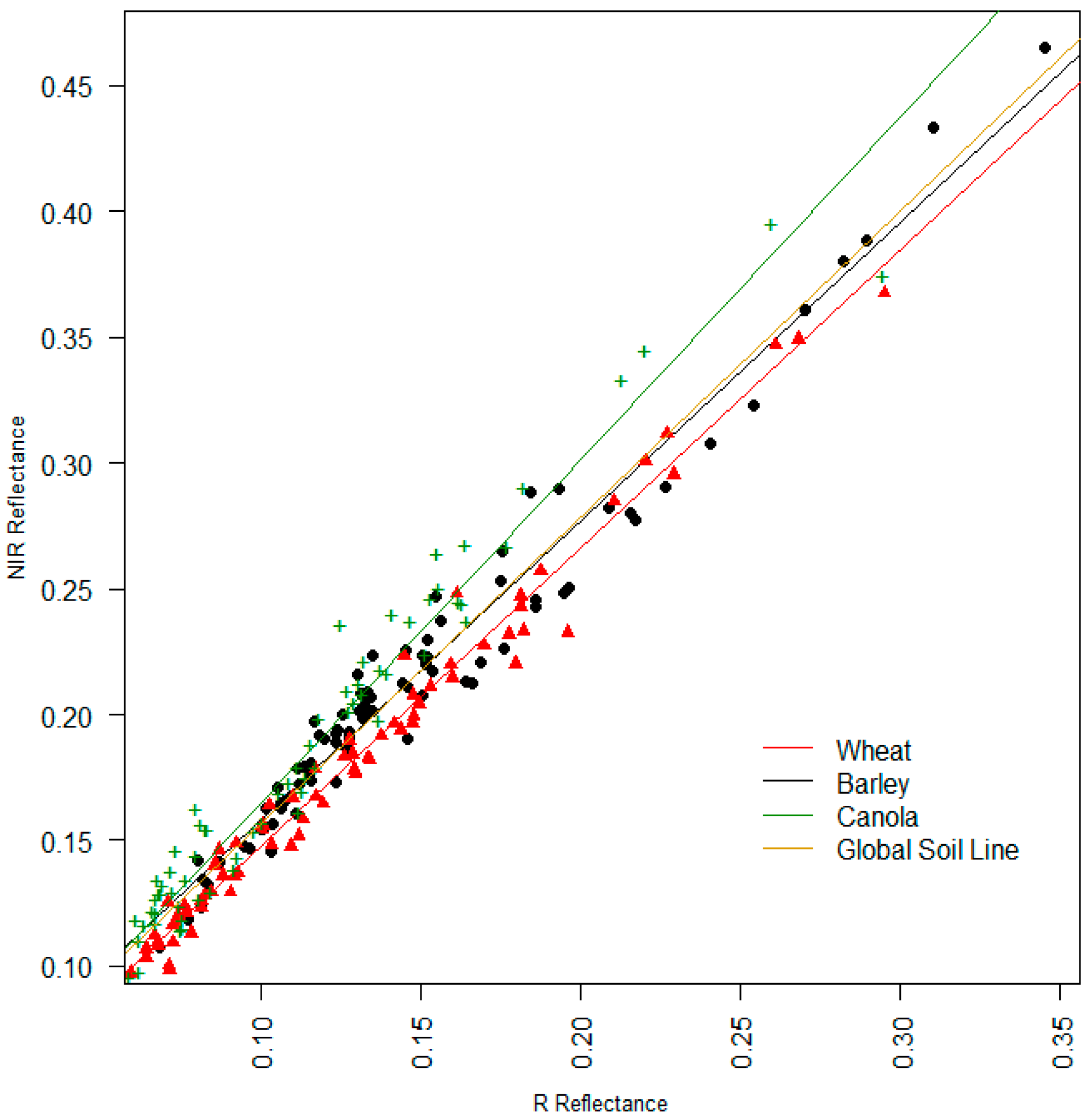
| Soils of Different Fields | a | b | R2 | RMSE |
|---|---|---|---|---|
| Wheat | 1.187 | 0.02862 | 0.9821 | 0.0089 |
| Barley | 1.188 | 0.03929 | 0.9632 | 0.0125 |
| Canola | 1.362 | 0.02875 | 0.9636 | 0.0134 |
| Global SL (Pool Data) | 1.22 | 0.03425 | 0.9555 | 0.0147 |
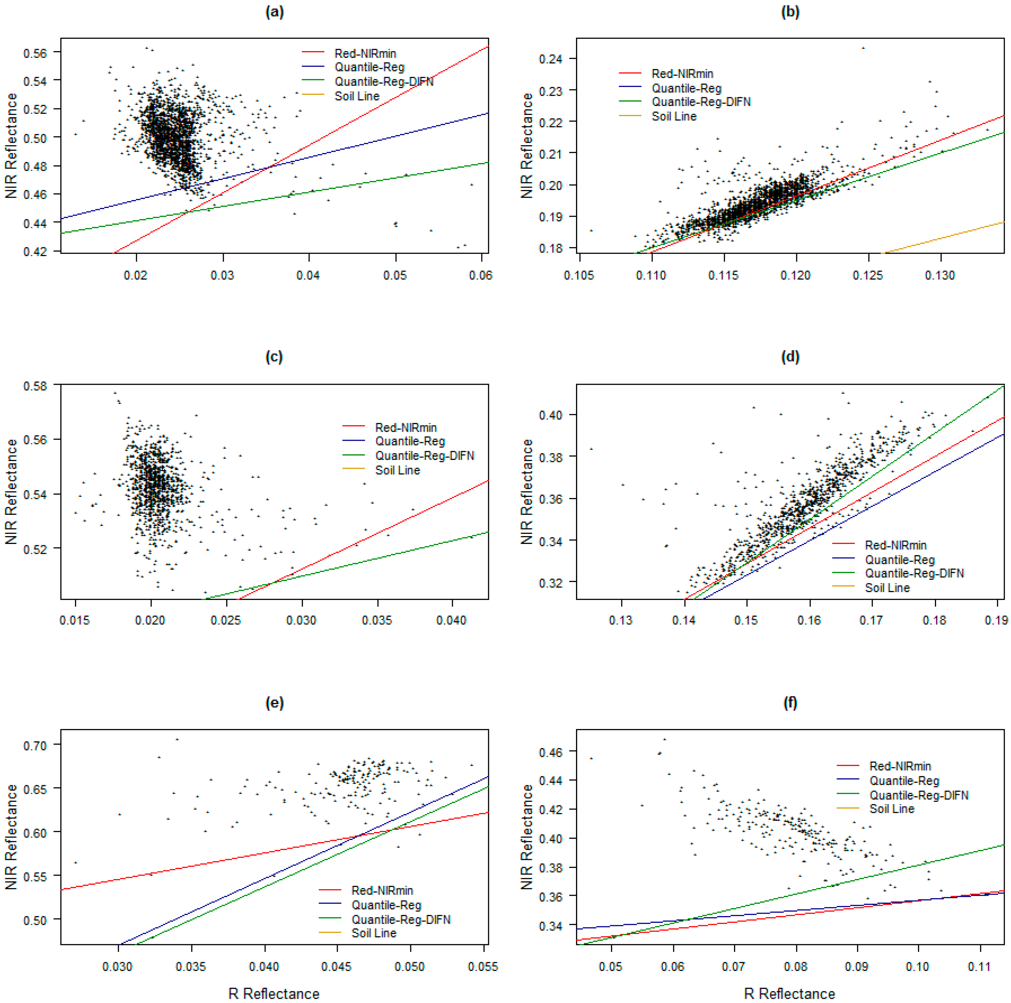
| Methods | (Red-NIRmin) | Quantile Float Tau | Quantile with Fixed Tau = DIFN | ||||||
|---|---|---|---|---|---|---|---|---|---|
| Date | Slope | Intercept | R2 | tau | Slope | Intercept | tau | Slope | Intercept |
| 2013/05/06 | 1.047 * | 0.047 * | 0.974 | 0.01 | 0.844 * | 0.100 * | 0.059 | 0.819 * | 0.121 * |
| 2013/06/07 | 0.796 * | 0.087 * | 0.981 | 0.02 | 0.617 * | 0.158 * | 0.016 | 0.623 * | 0.152 * |
| 2013/07/09 | 0.932 * | 0.074 * | 0.989 | 0.02 | 0.617 * | 0.158 * | 0.054 | 0.574 * | 0.191 * |
| 2013/08/10 | 1.067 * | 0.008 | 0.996 | 0.03 | 1.106 * | 0.042 * | 0.085 | 1.107 * | 0.059 * |
| Methods | Wheat | Barley | Canola | ||||
|---|---|---|---|---|---|---|---|
| Heading | Ripening | Heading | Senescence | Heading | Ripening | ||
| 2013/06/07 | 2013/08/10 | 2013/06/07 | 2013/07/16 | 2013/06/14 | 2013/07/09 | ||
| (Red-NIRmin) | Slope | 3.370 * | 1.782 * | 2.637 * | 1.711 * | 3.047 | 0.490 * |
| Intercept | 0.359 * | −0.018 * | 0.433 * | 0.072 * | 0.454 * | 0.308 * | |
| R2 | 0.903 | 0.867 | 0.962 | 0.994 | 0.340 | 0.994 | |
| Quantile float tau | tau | 0.075 | 0.089 | 0.010 | 0.004 | 0.022 | 0.010 |
| Slope | 1.500 | 1.500 * | 1.303 * | 1.648 * | 7.672 * | 0.364 * | |
| Intercept | 0.426 * | 0.015 * | 0.471 * | 0.076 * | 0.239 * | 0.321 * | |
| Quantile with fixed tau = DIFN | tau | 0.024 | 0.085 | 0.010 | 0.087 | 0.017 | 0.069 |
| Slope | 0.989 * | 1.500 * | 1.303 * | 2.068 * | 7.526 * | 1.000 * | |
| Intercept | 0.422 * | 0.0145 * | 0.471 * | 0.019 * | 0.236 * | 0.280 * | |
© 2016 by the authors; licensee MDPI, Basel, Switzerland. This article is an open access article distributed under the terms and conditions of the Creative Commons Attribution (CC-BY) license (http://creativecommons.org/licenses/by/4.0/).
Share and Cite
Ahmadian, N.; Demattê, J.A.M.; Xu, D.; Borg, E.; Zölitz, R. A New Concept of Soil Line Retrieval from Landsat 8 Images for Estimating Plant Biophysical Parameters. Remote Sens. 2016, 8, 738. https://doi.org/10.3390/rs8090738
Ahmadian N, Demattê JAM, Xu D, Borg E, Zölitz R. A New Concept of Soil Line Retrieval from Landsat 8 Images for Estimating Plant Biophysical Parameters. Remote Sensing. 2016; 8(9):738. https://doi.org/10.3390/rs8090738
Chicago/Turabian StyleAhmadian, Nima, José A. M. Demattê, Dandan Xu, Erik Borg, and Reinhard Zölitz. 2016. "A New Concept of Soil Line Retrieval from Landsat 8 Images for Estimating Plant Biophysical Parameters" Remote Sensing 8, no. 9: 738. https://doi.org/10.3390/rs8090738