Article

Do Agrometeorological Data Improve Optical Satellite-Based Estimations of the Herbaceous Yield in Sahelian Semi-Arid Ecosystems?

1
Centre de Suivi Ecologique, Rue Aimé Césaire x Léon Gontran Damas, BP 15532 Fann-Dakar, Senegal
2
Water, Environment and Development Unit, University of Liège, Avenue de Longwy B6700, 6700 Arlon, Belgium
3
Géosciences Environnement Toulouse (GET), Observatoire Midi-Pyrénées, UMR 5563 (CNRS/UPS/IRD/CNES), 14 Avenue Edouard Belin, 31400 Toulouse, France
4
Department of Geosciences and Natural Resource Management, University of Copenhagen, 1350 Copenhagen, Denmark
5
Centre Regional AGRHYMET, BP 11011 Niamey, Niger
*
Author to whom correspondence should be addressed.
Remote Sens. 2016, 8(8), 668; https://doi.org/10.3390/rs8080668
Submission received: 23 April 2016 / Revised: 26 July 2016 / Accepted: 10 August 2016 / Published: 18 August 2016
(This article belongs to the Special Issue Remote Sensing of Vegetation Structure and Dynamics)

Abstract

:
Quantitative estimates of forage availability at the end of the growing season in rangelands are helpful for pastoral livestock managers and for local, national and regional stakeholders in natural resource management. For this reason, remote sensing data such as the Fraction of Absorbed Photosynthetically Active Radiation (FAPAR) have been widely used to assess Sahelian plant productivity for about 40 years. This study combines traditional FAPAR-based assessments with agrometeorological variables computed by the geospatial water balance program, GeoWRSI, using rainfall and potential evapotranspiration satellite gridded data to estimate the annual herbaceous yield in the semi-arid areas of Senegal. It showed that a machine-learning model combining FAPAR seasonal metrics with various agrometeorological data provided better estimations of the in situ annual herbaceous yield (R2 = 0.69; RMSE = 483 kg·DM/ha) than models based exclusively on FAPAR metrics (R2 = 0.63; RMSE = 550 kg·DM/ha) or agrometeorological variables (R2 = 0.55; RMSE = 585 kg·DM/ha). All the models provided reasonable outputs and showed a decrease in the mean annual yield with increasing latitude, together with an increase in relative inter-annual variation. In particular, the additional use of agrometeorological information mitigated the saturation effects that characterize the plant indices of areas with high plant productivity. In addition, the date of the onset of the growing season derived from smoothed FAPAR seasonal dynamics showed no significant relationship (0.05 p-level) with the annual herbaceous yield across the whole studied area. The date of the onset of rainfall however, was significantly related to the herbaceous yield and its inclusion in fodder biomass models could constitute a significant improvement in forecasting risks of a mass herbaceous deficit at an early stage of the year.

Graphical Abstract

1. Introduction

In the Sahel belt south of the Sahara desert, an arid to semi-arid region, the vegetation is composed of a herbaceous layer dominated by annual grasses and scattered woody plants including bushes, shrubs and small trees, among which are several thorny species [1,2]. These areas provide the bulk of pastoral livestock feeding [3] and contribute to carbon sequestration, nutrient uptake and cycling, soil fixation and soil biologic activity, as well as water cycle regulation. In this context, an accurate evaluation of herbaceous mass yield at the end of the growing season is essential for ensuring the rational use of available resources and environmental sustainability. Vegetation indices derived from satellite data have been widely used to monitor Sahelian herbaceous productivity for about 40-years. After the severe drought of 1970s, the first applications of herbaceous yield estimation in Sahelian rangelands using the Normalized Difference Vegetation Index (NDVI) from the National Oceanic and Atmospheric Administration-Advanced Very High Resolution Radiometer (NOAA-AVHRR) were published and were pioneer studies in the field of applied remote sensing [4,5,6]. In the past two decades and with regard to the technological advances in sensor design for vegetation monitoring [7], new satellites such as the Satellite Pour l’Observation de la Terre-VEGETATION (SPOT-VGT) and the Moderate Resolution Imaging Spectroradiometer (MODIS)-TERRA/AQUA have been launched and more datasets have become available with higher spatial and denser temporal resolutions [8,9]. In addition to the NDVI, the Fraction of Absorbed Photosynthetically Active Radiation (FAPAR) in relation to surface processes such as photosynthesis [10] has been recognized as constituting a key variable in the assessment of vegetation status [11,12]. For this purpose, the metrics of the FAPAR seasonal dynamics are commonly used in environmental studies [13,14,15] and their potential for herbaceous mass monitoring in Sahelian rangelands has recently been endorsed by [16]. Most studies however, rely exclusively on satellite-based vegetation indices (e.g., [13,17]), with only a minority combining these indices with rainfall data, soil water status indicators and ground plant mass data.
Rainfall distribution is generally considered as the main driver of plant growth in the West African Sahel [18,19,20,21], although there are many other local drivers of plants’ photosynthetic capacity and spatial variability in the Sahel [22,23]. Among them, the supply of mineral nutrients such as nitrogen (N) and phosphorus (P) are major determinants of plant growth rate [24]. In the Sahel, N and P are the main limiting factors to plant production when rainfall is sufficient. For this reason, [25] proposed is the subdividing of the Sahel belt according to the 250 mm isohyet, with rainfall as the main limiting factor below 250 mm and the nutrients N and P the main limiting factors above 250 mm annual rainfall. The wide temporal variability of N and P however, in relation to the soil moisture regime and the absence of reliable information on their spatial distribution across Sahelian regions makes it difficult to include this information in statistical modeling approaches. In contrast, comprehensive rainfall data has become increasingly accessible for use in the Sahel through the development of satellite-based products such as the Tropical Applications of Meteorology using SATellite (TAMSAT) data and ground-based observations [26], the Famine Early Warning System NETwork (FEWS NET) Rainfall Estimate (RFE) [27] and the African Rainfall Climatology (ARC) [28]. The use of rainfall data as the overall driver of plant growth is supported by the high variability of Sahelian herbaceous productivity, which is difficult to predict in time and space [29,30]. Not all rainfall water however, is directly available to plants. Rainfall water availability is mediated by the redistribution (i.e., run-off/run-on) on the soil surface in relation to soil physical characteristics (i.e., structure and texture), to topography [25] and to the physical nature of the canopy [31]. This could help explain the poor relationship observed between herbaceous yield and annual total rainfall in the Sahelian rangelands of Niger and Mali [32,33]. It justifies the concept of a water requirement index (also called a water satisfaction index or a water requirement satisfaction index, WRSI) developed and implemented through a soil water balance model named the Crop Specific Water Balance (CSWB) by the Food and Agricultural Organization (FAO) of the United Nations. With this model, the water balance of a given crop can be calculated in time increments, usually 10 days (i.e., dekad), as presented in Equation (1) [34]. Then, when filled with complementary parameters, the CSWB model produces a set of water status indicators generally used to assess the effect of weather conditions on crop development and yield [35,36].
W d = W d 1 + R ETm ( r + i )
where,
  • Wd: amount of water stored in the soil at the end of the dekad (d)
  • Wd–1: amount of water stored in the soil at the end of the previous dekad (d–1)
  • R: cumulated rainfall during the dekad
  • ETm: maximum evapotranspiration in the decadal period
  • r: represents the water losses due to runoff in the decadal period
  • i: represents the water losses due to deep percolation in the decadal period
For its agricultural monitoring activities, FEWS NET developed a grid cell-based modeling environment from the FAO’s CSWB [37]. The established geospatial model, GeoWRSI, was then enhanced by [38] for West Africa’s Sahelian rangelands [39]. Plant production models established solely from the absorbed PAR, as mentioned earlier and according to [40], neglect the direct effects of other factors such as water availability and nutrient shortage on plant growth. Models including both soil moisture (i.e., soil water status indicators) and the metrics of FAPAR seasonal dynamics are therefore expected to overcome FAPAR-related problems (e.g., saturation and cloud contamination) and to improve herbaceous standing mass estimations. In such models, agrometeorological data introduce information about soil water availability, whereas FAPAR metrics provide information on herbaceous productivity and species patterns not taken into consideration by the agrometeorological component [41].
In this context, the overall aim of our study was to predict the herbaceous yield across the arid to sub-humid areas of Senegal. The originality of the study was the combination of satellite-based rainfall estimates, agro-ecological data and satellite-derived FAPAR metrics using a machine learning approach. The more specific objectives were to: (i) develop three herbaceous models based only on FAPAR metrics, only on agrometeorological variables and on the combined FAPAR and agrometeorological variables; (ii) conduct a spatio-temporal comparison of model outputs; and (iii) analyze the relationship between herbaceous yields and the onset/end of season metrics calculated from FAPAR and satellite-based rainfall data for early warning purposes.

2. Materials and Methods
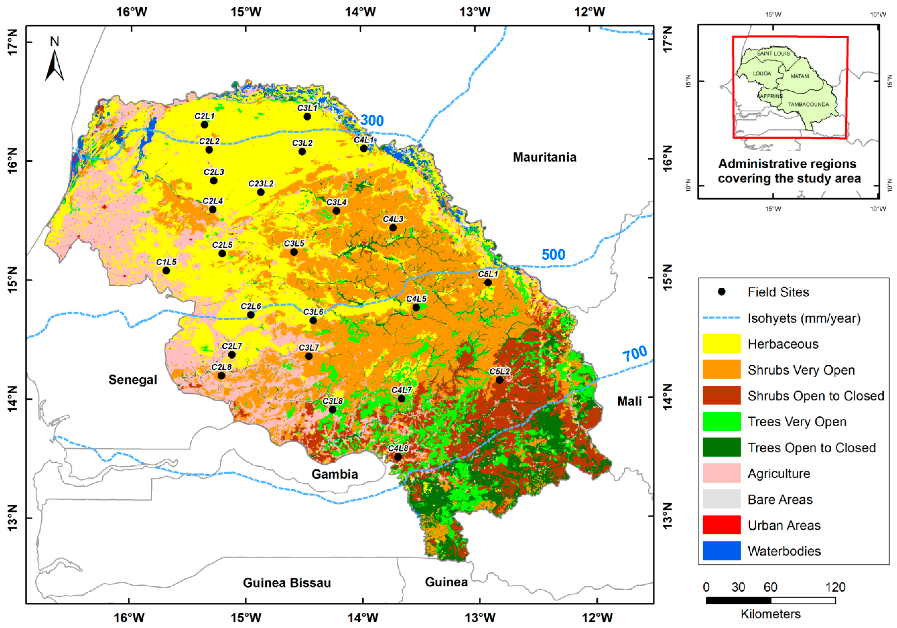
2.1. Study Area

The study area covered 15 districts belonging to five administrative regions (i.e., Saint-Louis, Matam, Kaffrine, Louga and Tambacounda), with a total area of 125,000 km2 (Figure 1). The area lies in the Sahelian and northern Sudano-Guinean zone of Senegal between 16.69°N and 12.63°N latitude and 16.74°W and 11.86°W longitude. It includes all natural grazing areas of the pastoral domain as defined by [42], as well as some croplands, including fallows. The mean annual precipitation varies between 200 and 980 mm from north to south, with reference to the FEWS NET rainfall estimates for the 2000–2015 period [43,44]. The rainy season, driven by the West African monsoon, is unimodal, occurring over 3–5 months between June and October. The studied area includes different ecoregions, with a prevalence of red-brown sandy soils, ferruginous tropical sandy soils, leptic, gley and vertic soils [45,46]. Typical of the Sahel, the herbaceous vegetation is particularly dependent on the intra-seasonal rainfall distribution [47] and is dominated by annual plants with C4 photosynthesis [48]. According to the Centre de Suivi Ecologique (CSE) [49,50], the northern zone (≤300 mm annual rainfall) is characterized by Poaceae such as Chloris prieurii, Aristida mutabilis and Dactyloctenium aegyptium, as well as legumes such as Alysicarpus ovalifolius and Zornia glochidiata, whereas in the central zone (between 300 and 500 mm) the characteristic species are Zornia glochidiata (Fabaceae) and Schoenfeldia gracilis, Pennisetum pedicellatum and Eragrostis tremula (all Poaceae). Towards the south, Andropogoneae species such as Andropogon pseudapricus and A. amplectans are the most common species. Other species, such as Spermacoce stachydea (Rubiaceae), Cassia obtusifolia (Fabaceae) and Fimbristylis exilis (Cyperaceae), occur irregularly, depending on the terrain morphology (e.g., depressions) and human and livestock influence. The studied area contains nine land cover classes that, when excluding cropped lands, coincide with woody plant density, which increases from north to south (Figure 1, Table 1). These nine classes were constituted by aggregating the 60 classes of the original land cover database of Senegal [51] and more or less corresponded with those used by [52] for analyzing land cover change in Senegal between 1990 and 2005.

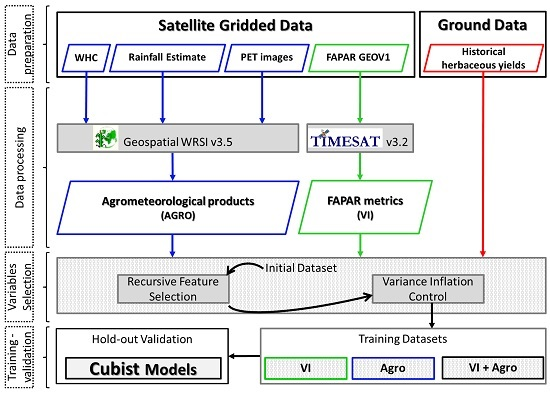
2.2. Data and Processing

2.2.1. Historical Field Herbaceous Yields

The in situ herbaceous mass data used in this study for the calibration of the models were collected annually from 2000 to 2015 (except for 2004) from 24 field sites located in free access natural rangelands, as shown in Figure 1 (black dots). The sites were selected away from the main water points and pastoral camps in order to avoid heavy grazing. Each field site covered a 3 × 3 km² homogeneous area and represented the most common land cover classes. Above-ground herbaceous mass was measured towards the end of the growing season, in early October. The technique used was the stratified sampling line originally proposed by the International Livestock Centre for Africa (ILCA) for monitoring pastoral ecosystems in the Gourma of Mali [55]. Along a 1000 m transect, four strata (bare soil, and low, medium and high herbaceous mass production) were identified. Then, taking into account the variability of herbage mass in the three covered strata, between 35 and 100 plots (each 1 m2) were sampled randomly along the transect line and fresh herbaceous mass was cut and weighed within each plot. After re-sampling, three samples for each stratum (i.e., nine samples per site) were kept for drying. The dry matter rate obtained by dividing the dry herbaceous mass weight by the fresh mass weight, as well as the relative frequency along the 1000 m transect, were then used to calculate the herbaceous mass yield in kg·DM/ha, first for each of the three strata and then for the site by adding them together. Note that the biomass data were not regularly collected in all monitoring sites due to occasional lack of logistics or the early passage of bush fires before field measures [16]. For more detailed information on the overall herbaceous mass collection, see [16].

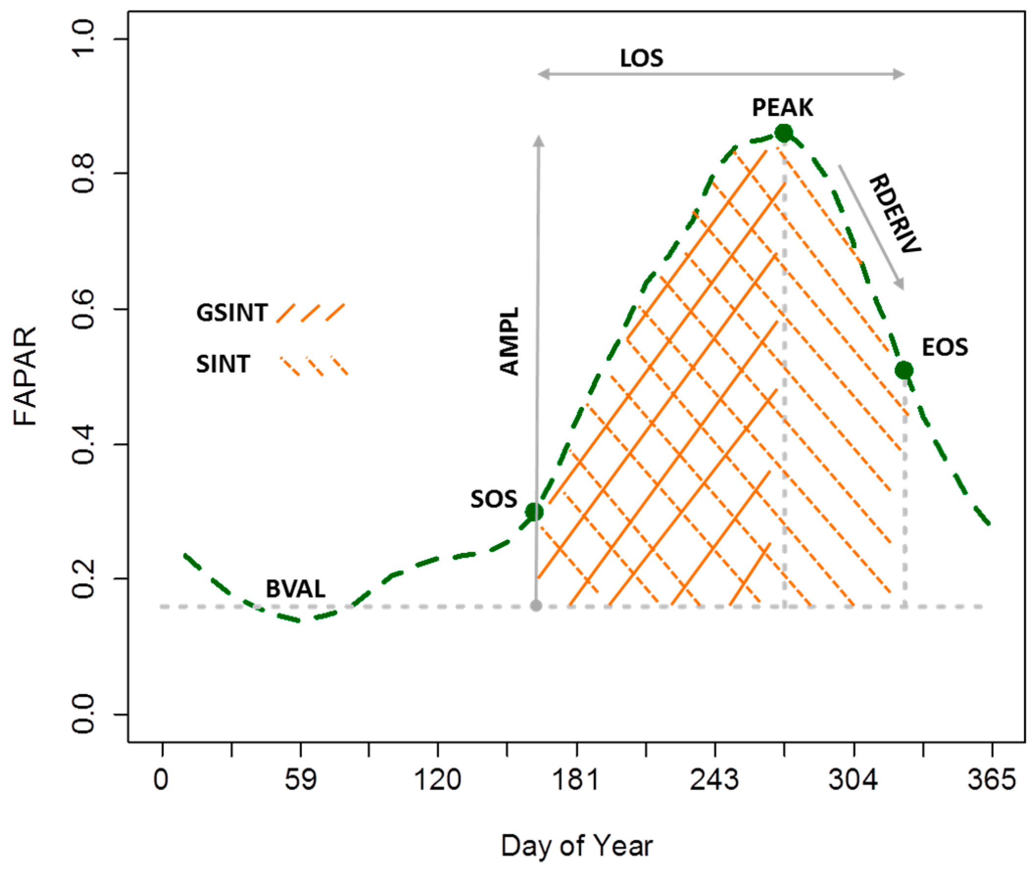
2.2.2. FAPAR Vegetation Dynamics and Calculated Metrics

GEOV1 Copernicus Global Land FAPAR runs from 24 December 1998 to the present day at a ground sampling distance of 1/112° (about 1 km at the Equator) and 10-day steps [56]. Derived from the SPOT-VEGETATION (from 2000 to 2013) and Proba-V (for 2014 and 2015) instruments, this product is freely available on http://land.copernicus.eu/global. For detailed information on the principles used to estimate the GEOV1 FAPAR product, see [10].
In order to calculate seasonal metrics, the GEOV1 FAPAR time series were filtered using the Savitzky-Golay (SG) fitting method available via TIMESAT software [16,57]. Filtering is essential in semi-arid areas such as the Sahel, where many factors (e.g., clouds, aerosols, shadows, surface water) tend to produce noisy and erroneous FAPAR values [58,59]. From the filtered FAPAR time series, eight metrics were retrieved with TIMESAT and used in this study (Figure 2): the start of the plant growth season (SOS); the end of the season (EOS); the length of growing season (LOS); the maximum FAPAR value over the season (PEAK); the amplitude (AMPL) corresponding to the difference between PEAK and the averaged left and right minimum values over the ongoing annual cycle (BVAL); the small integrated FAPAR (SINT) from SOS to EOS and above BVAL; the small integrated FAPAR from SOS to PEAK time and above BVAL (GSINT); and the decreasing rate during the senescence phase (RDERIV). All these metrics have been described by [15,16], except for GSINT, which was computed to include information during the green-up phase. SOS and EOS are essential for calculating the cumulated FAPAR metrics and were set to occur at 20% and 50% of the seasonal AMPL before and after the peak value, respectively [16]. All the metrics were derived for each year between 2000 and 2015 on a pixel basis and 1 km spatial resolution. The annual values were then averaged for each site over an area of about 3 × 3 km² to match, as far as possible, the spatial sampling of the ground data.

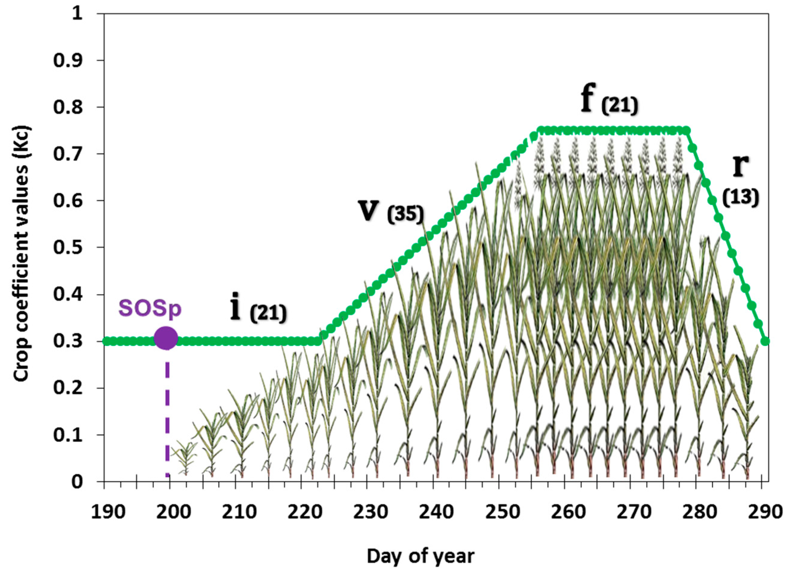
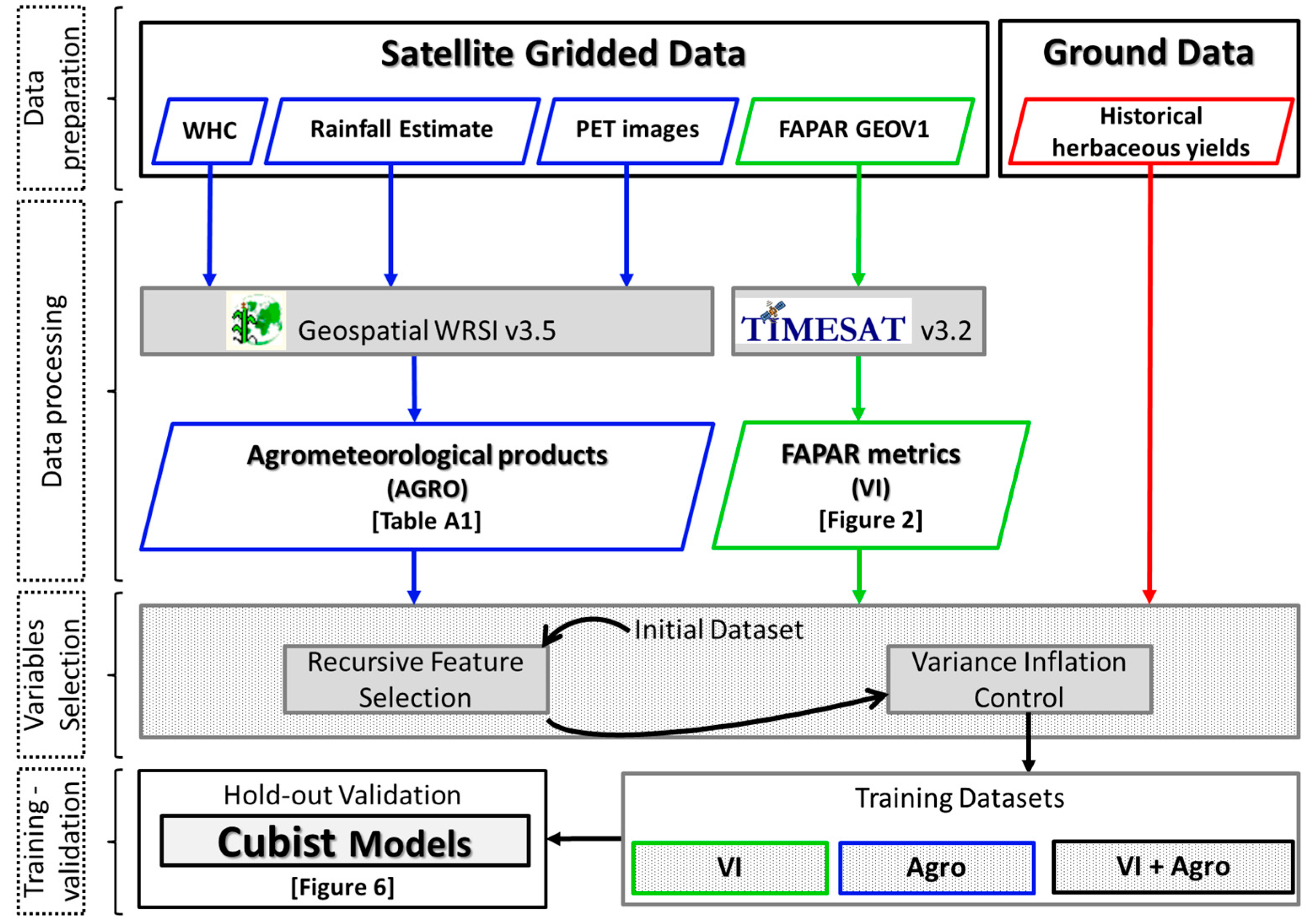
2.2.3. Obtaining Agrometeorological Data

Agrometeorological data was calculated using the GeoWRSI model of FEWS NET adapted to a grid cell-based modeling environment [37] from the original water balance algorithm of FAO [35]. As noted by [60], the GeoWRSI model was enhanced and extended into an operational mode for Africa, Central America and Afghanistan after the work by [61]. The WRSI indicator (Equation (2)) is the ratio of seasonal actual crop evapotranspiration (AETc) to the seasonal crop water requirement, which is equivalent to potential crop evapotranspiration (PETc) [60]. AETc represents the actual amount of water withdrawn from the soil water reservoir by vegetation transpiration and soil evaporation [60,62] and PETc is the cumulative optimum crop water requirement as met by rainfall and soil moisture for a given accumulation period [39]. Following [60], the PETc at a given time in the growing season is calculated by multiplying the potential evapotranspiration (PET) by the crop coefficient (Kc), as in Equation (3). The AETc is determined by a set of functions integrating rainfall amount (PPT), plant available water (PAW), critical soil water level (SWC), soil water holding capacity (WHC), crop root depth (RD) and soil water content (SW) at the end of the study period. SW can be estimated using a soil water balance [60,63] with Equations (4).
WRSI =   AETc   PETc × 100
PETc = Kc × PET
SW i = SW i 1 + PPT i AETc i
where i corresponds to the time step.
For more information on the development and parameterization of the GeoWRSI model, see [60,61]. The main parameters needed to run the model are PPT, PET, WHC and Kc values. We ran the model in this study using the Africa-wide blended satellite-gauge rainfall estimate images implemented by the Climate Prediction Center (CPC) of NOAA [43,44] and the global PET images estimated from the 6-hourly numerical meteorological model output using the Penman-Monteith equation [64]. Rainfall and PET images were downloaded in dekadal time steps with a 0.1 degree (about 10 km) and 1 degree (about 110 km) spatial resolution respectively, from the ftp server of the Climate Hazard Group for the archive data between 2000 and 2010 [65] and the FEWS NET server for the latest data between 2011 and 2015 [66]. The WHC image shows the spatial variation of easily available water capacity in the upper 100 cm, based on soil physical characteristics [37] and was obtained from the FAO digital soil map of the world [67] with a 0.1 degree spatial resolution. Kc values correspond to those proposed by [68] for the extensive grazing pastures in semi-arid climates (Figure 3). These values were chosen with the assumption that the study area is uniform in hydro-climatic conditions and after a visual analysis of WRSI variable which showed the most reasonable distribution for a median year regarding rainfall conditions.
The rainy season onset date (SOSp) was calculated for each modeling grid cell using the criteria of at least 25 mm of rainfall received over a given dekad, followed by a total of 20 mm for the next two dekads as applied by [37] after [69]. The end-of-season date (EOSp) occurred when a climatological ratio between rainfall and potential evapotranspiration (i.e., PPT < PET/2) was observed [60]. SOSp and EOSp were in turn used to calculate the herbaceous vegetation WRSI. In addition to WRSI, SOSp and EOSp, we calculated 12 other agrometeorological variables for the growing periods of each year (Table A1), particularly actual evapotranspiration (AET), water deficit (WDEF) and water surplus (WSUR) that accumulated during each of the four herbaceous vegetation growth phases (illustrated in Figure 3): initial (i); vegetative (v); flowering (f); and ripening (r). The seasonal fractions assigned to these four phases were 23%, 39%, 23% and 15% respectively, (numbers taken from the Sahelian Transpiration, Evaporation, and Productivity [STEP] model) [40]. The computed rainfall variables corresponded to the seasonal amount accumulated from the start to the end of the rainy season (PPTc) and the mean rainfall from the start to the end of the season (PPTm). All the agrometeorological images were re-sampled to a 1 km resolution in order to match the FAPAR metrics using a bilinear interpolation method.

2.3. Methods

The overall approach applied for elaborating the estimation models of herbaceous yield is presented in Figure 4.

2.3.1. Explanatory Variable Selection for Herbaceous Mass Estimation

Over-fitting is a major drawback of machine learning methods [70] and can occur when there is a strong relationship between the explanatory variables. In order to avoid over-fitting, only relevant variables with no significant collinearity should be kept in a model. Redundant predictors can trigger substantial instability in a model’s coefficients. Wrapper methods (e.g., backward and forward) are widely used in the search procedure for predictors’ selection in environmental studies (e.g., [71,72,73]). As reported by [74] and [75] however, the principle of these methods lies in repeated hypothesis tests with the same data, which invalidates many of their statistical properties. In order to overcome this drawback, [76] proposed the recursive feature elimination procedure. This method is a sequential backward selection approach [77] that avoids refitting many models at each step of the search by including an importance-ranking criterion instead [75]. The recursive feature elimination algorithm available with R software [78] was used to identify less pertinent variables from the original dataset. In this algorithm, the random forest function [79] was used to compute the importance of the variables (i.e., mean decrease in accuracy when a variable is permuted) and rank them over subsets. The procedure’s output with variables ranked from most to least important was then evaluated in order to eliminate interrelated explanatory variables [15], using the Variance Inflation Factor (VIF) indicator (Equation (5)). The least important variables with a VIF ≥ 10 [80] were eliminated one by one. This process was repeated until the VIF for all remaining variables was below 10.
VIF = 1 / ( 1 R ² j )
where R²j is the correlation coefficient for the regression of each variable with the remaining ones.

2.3.2. Rule-Based Regression Tree and Model Building

The classification and regression trees (CART) approach, also called decision trees, is a data mining method used to identify patterns between a dependent variable and several independent predictor variables [81]. CART models can be used for either classification or regression, where classification trees predict classes and regression trees predict a continuous response [79,82,83]. We used the Cubist program [78], providing rule-based models using regression trees because the modeled herbaceous mass was continuous. Each tree was reduced to a set of conditional rules retrieved from the most important predictor variables [84]. These rules partitioned the independent variables (FAPAR metrics and/or agrometeorological products) into smaller groups and each of which was linked to a multiple linear regression model that predicted the dependent variable (herbaceous mass) [75]. This algorithm, based on if/then rules, is well suited for Sahelian ecosystems, which are characterized by high spatial heterogeneity in terms of soil type and fertility, rainfall mediated by run-off/run-on and species composition. The initial dataset was randomly separated into a ‘training set’ and a ‘verification set’ containing 70% and 30% of the data respectively. Then a simple check was made to ensure that all land cover classes are represented in the two sub-datasets. Model learning was done with the training set, using a boosting-like scheme called ‘committees’ [84], where each committee member corresponds to one regression tree. The number of committees was tuned by applying the commonly used 10-fold cross-validation in the model’s performance estimation [85,86]. All instances of the initial dataset were used and the cross-validated root mean squared error (RMSE) applied in order to obtain the best value of the committee number. It should be noted that for each committee after learning, a subsequent member (multiple linear regression model) adjusts, for inaccuracies, in the prediction of the previous one and the final predicted value is a simple average of all predictions from the various members [75,81,84]. For comparative purposes, three cubist models were established: (i) the Vegetation Index-model (VI-model) including only FAPAR metrics; (ii) the Agrometeorological-model (AGRO-model) computed with agrometeorological variables; and (iii) the VIAGRO-model including both FAPAR and agrometeorological data.

2.3.3. Model Verification, Error Analysis and Yield Anomaly Computation

Model accuracy verification was performed using an independent set of samples that were not used (i.e., hold-out) for the training of the model. The Cubist models were trained using the training set (207 samples) and then used to estimate the herbaceous yield values of the verification set (90 samples). The validation accuracy was retrieved using the observed and predicted herbaceous yield of the verification set. The quality of the models was assessed by the RMSE and mean absolute error (MAE). The anomaly values were calculated pixel-wise by the ratio (in percentage) of the difference between the actual and long-term average of the herbaceous yield (or rainfall) and the 15-year long-term average.

3. Results

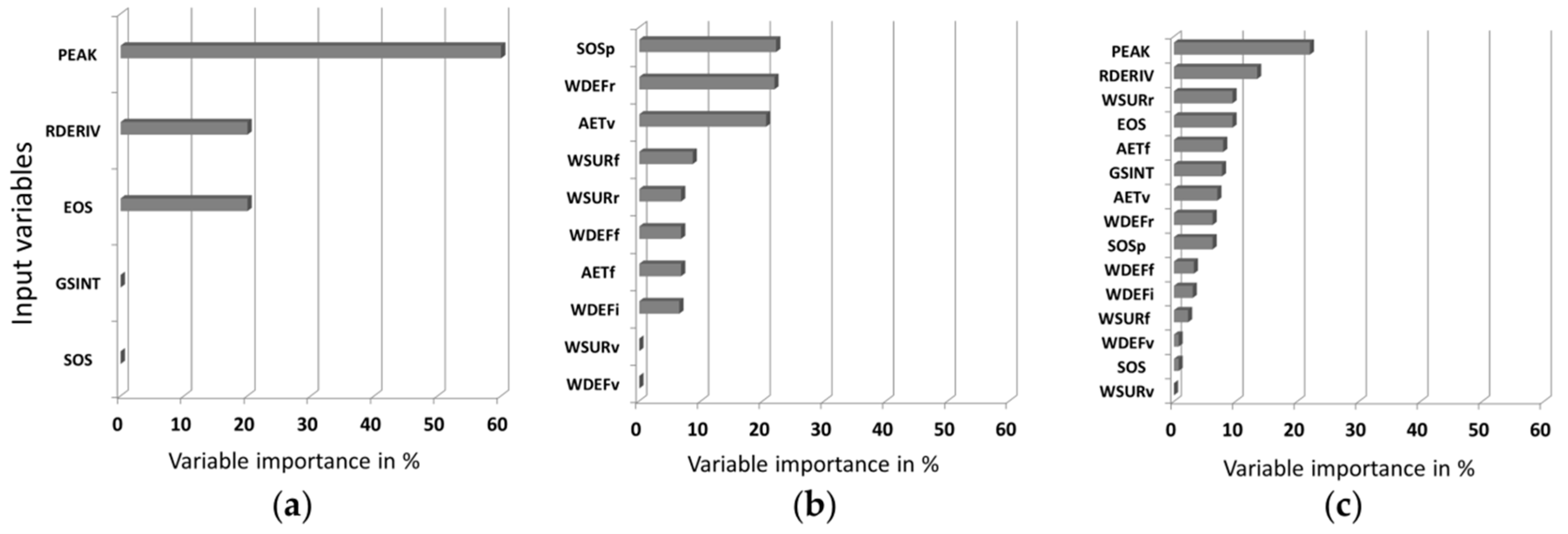
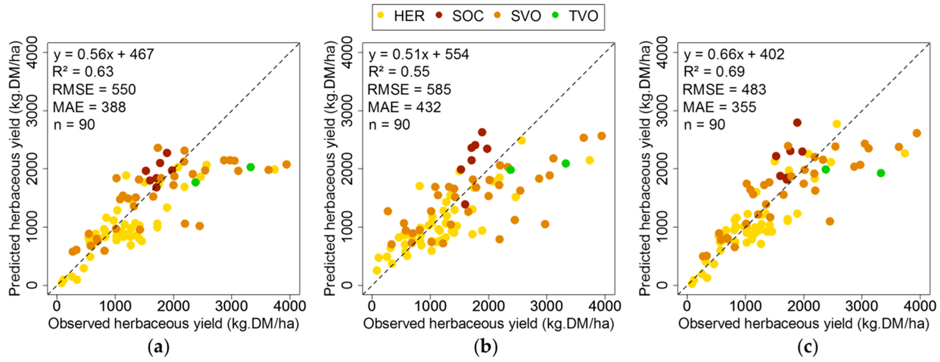
3.1. Variable Selection and Model Development

After removing all the interrelated variables, a final dataset of 15 explanatory variables remained and were used for model development (Figure 5c). Three models were developed for estimating herbaceous yields using: (a) only FAPAR metrics (VI-model); (b) agrometeorological data (AGRO-model); and (c) both FAPAR metrics and agrometeorological data (VIAGRO-model). The set of variables used for each model is shown in Figure 5 and the model performance is shown in Figure 6.
The contribution of the input variables varied with each model. For the VI-model, the PEAK variable was the most important, followed by the right derivative (RDERIV) and EOS (Figure 5a). GSINT and SOS were the least pertinent variables as neither was used in model conditions or equations. In the AGRO-model, the SOSp and water deficit during ripening (WDEFr) were the most important variables, whereas the least important were water deficit (WDEFv) and water surplus (WSURv) during the growth stage. The most important variable in the VIAGRO-model was PEAK, followed by RDERIV. The SOS had little or no importance in the VI-model and VIAGRO-model, unlike the SOSp, which played a major role in AGRO-model and VIAGRO-model. The validation statistics of the three models are given in Figure 6. The VIAGRO-model showed the best performance with R² = 0.69, RMSE = 483 kg·DM/ha, MAE = 355 kg·DM/ha and slope = 0.66. The VI-model performed less well with R² = 0.63; RMSE = 550 kg·DM/ha; MAE =388 kg·DM/ha; slope = 0.56, followed by the AGRO-model, R² = 0.55; RMSE = 585 kg·DM/ha; MAE = 432 kg·DM/ha; slope = 0.51.

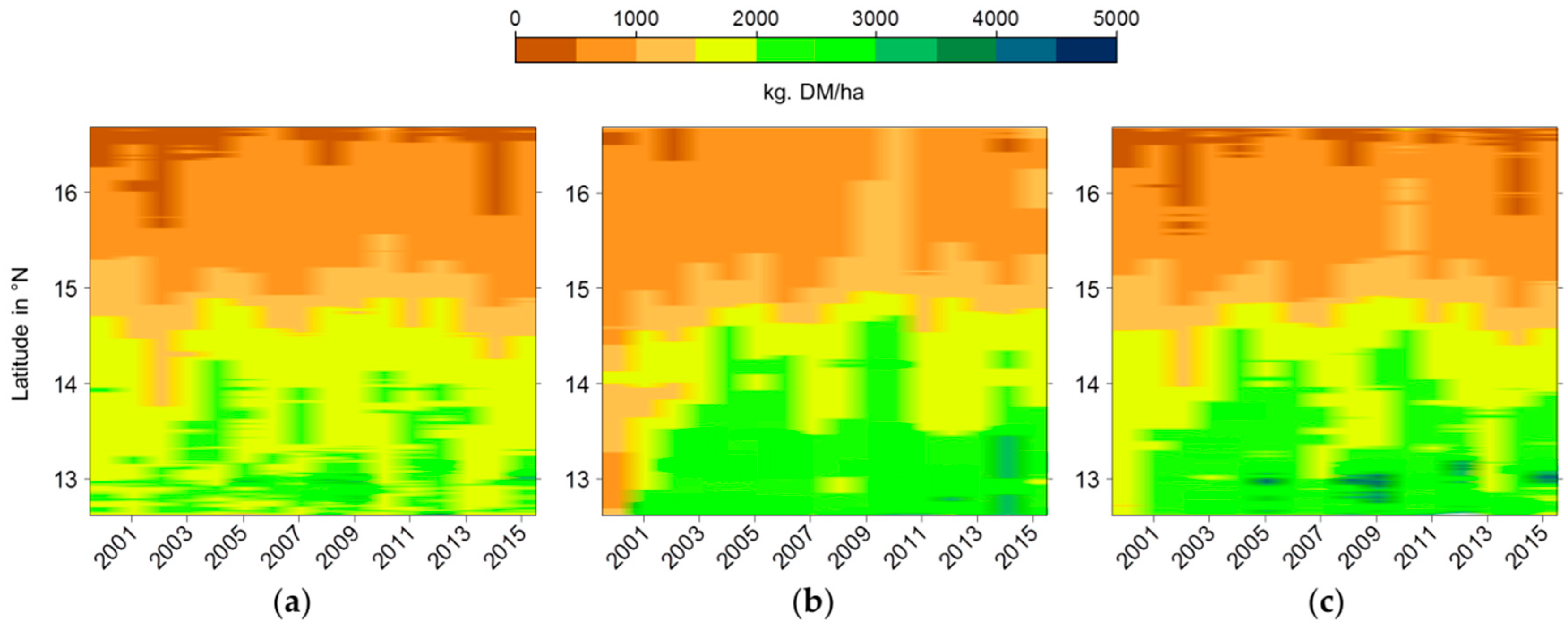
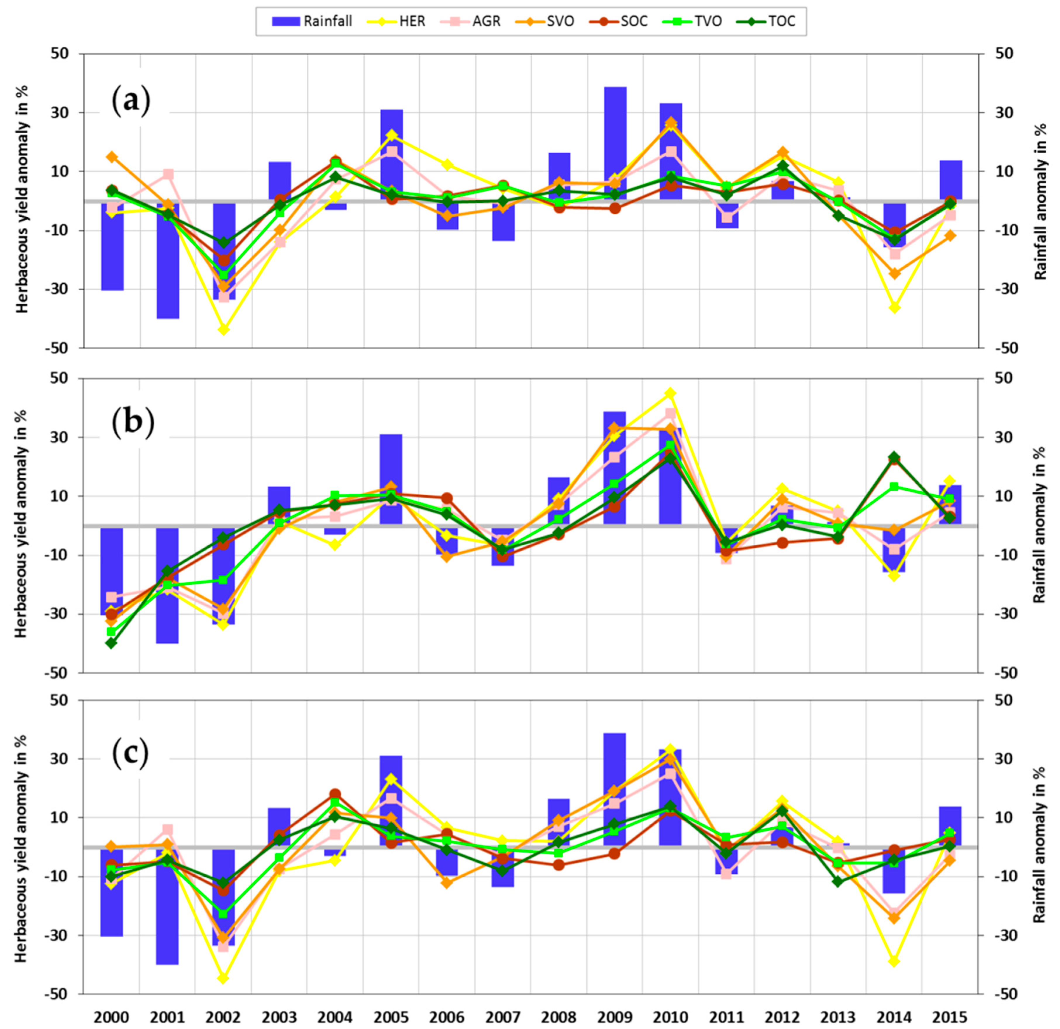
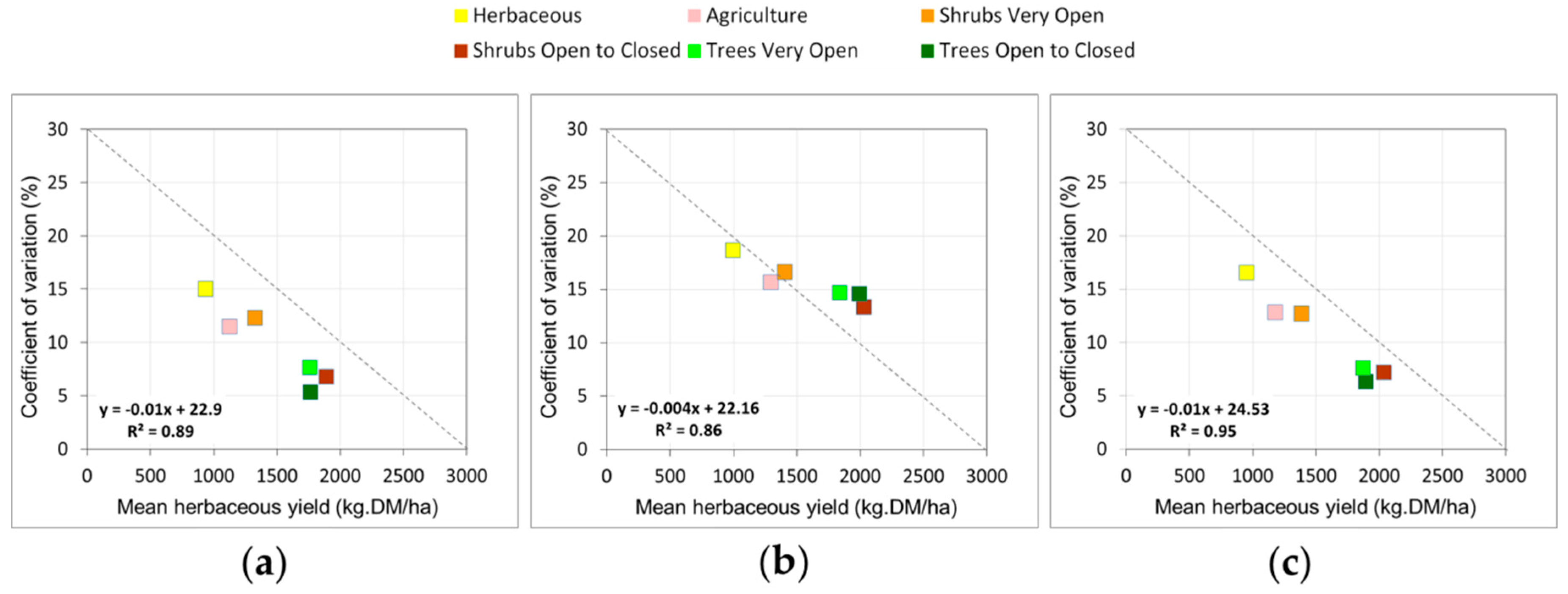
3.2. Spatio-Temporal Comparison of the Models’ Output

All the established models provided herbaceous yield estimations with values increasing along a north-south gradient in the 2000–2015 period (Figure 7). The VI-model however, gave generally lower estimations than the two other models. Particular years, such as 2002 and 2014 when there was a considerable deficit in herbaceous mass production, were reflected well in both the VI-model and VIAGRO-model. The year 2010 however, was characterized by a high herbaceous mass production, which was clear in the AGRO- and VIAGRO-model estimations but less so in the VI-model. Overall, the VI-model underestimated high values, especially in the more southern regions; this drawback was corrected in the VIAGRO-model.
As an indicator of the inter-annual variability of vegetation [33,87], the coefficient of variation (CV) of the herbaceous yield estimated by the three models over a 16-year period was used to assess the temporal variations in herbaceous yield across natural vegetation and agricultural land cover classes (Figure 8). The inter-annual variations in herbaceous yield differed among the land cover classes. The AGRO-model showed the highest CV values, followed by the VIAGRO-model and the VI-model. For all the models, the HER class had the highest temporal variability, with an average CV of 17%, followed by SVO and AGR, with 14% and 13%, respectively. The lowest inter-annual fluctuations were observed in land cover classes with high herbaceous yields and woody cover, such as TVO (CV = 10%), TOC (CV = 9%) and SOC (CV = 9%).
The herbaceous yield anomalies were assessed (Figure 9) and were generally in agreement with rainfall anomalies across the studied land cover classes, particularly for extreme years such as 2002 and 2010. Some discrepancies between the VI-model and the other two models were observed in 2000 and 2014. The VI-model showed a positive anomaly for SVO, whereas the AGRO- and VIAGRO models provided negative and no anomalies for the same class in 2000. For 2014, the AGRO-model provided positive anomalies for the SOC, TVO and TOC classes, whereas the VI-model and VIAGRO-model provided negative anomalies. As shown in Figure 9, the VIAGRO-model generally provided a blended estimation of the anomalies compared with the VI-model and AGRO-model.

3.3. Season Onset/End Derived from FAPAR and Rainfall Data

As observed in Section 3.1, the onset/end metrics estimated from the FAPAR seasonal curve (indicating the plant growing season) and rainfall data (indicating the rainy season) played different roles in model establishment (Figure 5), contrary to what was expected. The onset and end of the growing season (SOS and EOS from FAPAR) and of the rainy season (SOSp and EOSp from rainfall) are illustrated in Figure 10. The mean SOS and SOSp dates were delayed from the southern to northern land cover classes along the climatic gradient, reflecting the progression of the West African monsoon. With regard to the median values in boxplots, the growing season started in June for the three classes (SOC, TVO and TOC) located mainly in the south, whereas for the AGR, SVO and HER classes, the growing season started in July. The SOS occurred mainly in the same dekad as the SOSp for all land cover classes except HER, where it started about a dekad early (Table A2). The end of the growing season was concentrated between late October and November, being later towards the south. On average, the EOS occurred about 2 dekads after the EOSp which occurred about late October. The EOS varied, occurring early for the HER class but late for TOC in November.

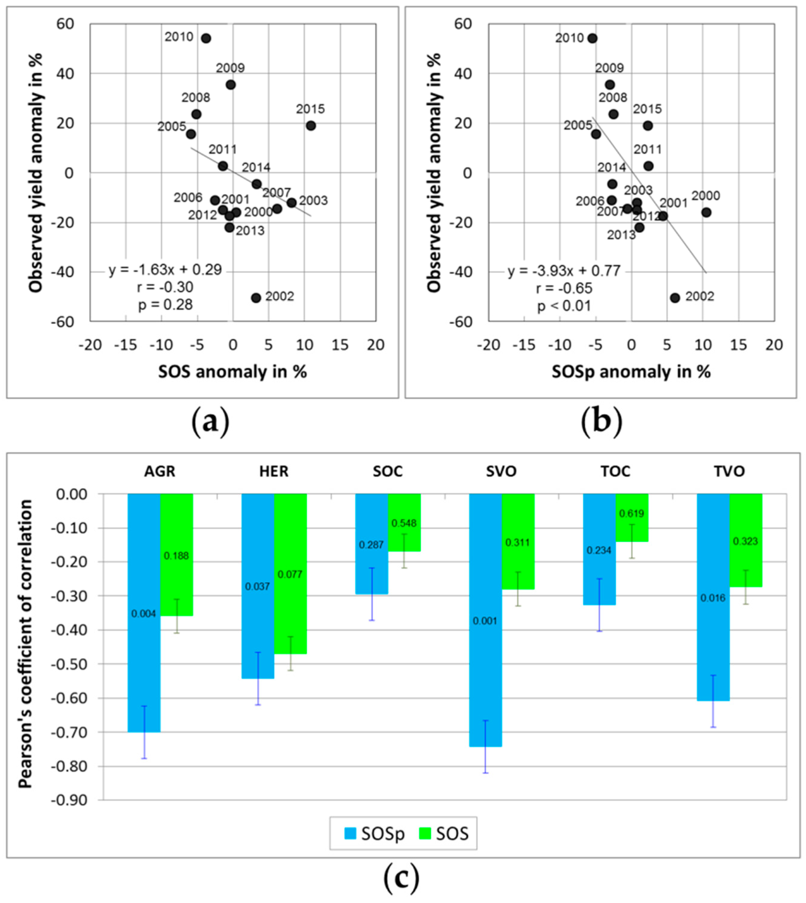
3.4. Linkage between Start of the Growing/Rainy Season and Annual Herbaceous Yield

This section analyzes the relationship between SOS and SOSp and the herbaceous yield. The range of the SOS and SOSp anomalies was narrow (−5% to +10%) compared with the herbaceous yield anomalies (−60 to +60%). A very weak and non-significant relationship (r = −0.30% and p = 0.28) was observed between the SOS and in situ herbaceous yield anomalies which were averaged over the study area (Figure 11a). In contrast, the meteorological variable SOSp had a highly significant relationship with observed herbaceous yield anomalies (r = −0.65 and p < 0.01) (Figure 11b). This was confirmed over all the land cover classes where SOSp achieved r = −0.74 for SVO, whereas the maximum r value for the SOS metrics was −0.47 registered for HER (Figure 11c). For all the land cover classes, there was no significant relationship (at the 95% significance level) between SOS and the observed herbaceous yield anomalies. The weakest relationships for the two metrics were observed for the open to closed classes dominated by either shrubs or trees (i.e., SOC and TOC respectively), being insignificant for both SOS and SOSp.

4. Discussion

4.1. Model Development and Output Comparison

All three models gave a reasonable performance. The VIAGRO-model (including both FAPAR and agrometeorological variables) however, outperformed the models based solely on FAPAR metrics (VI-model) and agrometeorological variables (AGRO-model). Among the three models, the AGRO model had the weakest performance, which could be related to the fact that all applied variables are independent of internal factors (i.e., the influence of grazing) whereas all FAPAR metrics as well as the field data are influenced by grazing over time. All the models showed a coherent distribution of the estimated herbaceous yield, with values increasing along the north-south gradient, together with decreasing inter-annual variability. The saturation effect has always been a drawback in the optical vegetation products in relation to the high productivity of vegetation mass [88,89,90,91,92] and was consequently observed in VI-model. The simultaneous use of agrometeorological data and FAPAR metrics mitigated the saturation effect, being more sensitive to high greenness values. However, high biomass values (>3000 kg DM/ha) are still underestimated in the AGRO- and VIAGRO-models, which could be related to the few sites sampled in densely vegetated classes within the global dataset (see Table 1). Hence there is a need to establish more sites in southern Senegal in order to achieve greater accuracy of the herbaceous yield forecasting over the whole country. The agrometeorological data also reduced the discrepancy between herbaceous mass and FAPAR values, with the VIAGRO-model having a smaller scatter of low values and high values closer to the 1:1 line (see Figure 6). The contribution and significance of the input variables varied among the models. In the VIAGRO-model and VI-model, the FAPAR PEAK was the most important variable, whereas SOS was the least important. The relevance of PEAK in Sahelian grasslands has been demonstrated by [14,16]. The most important variable for the AGRO-model however, was SOSp and the least important was WDEFv. The latitudinal variation of the herbaceous yield estimated by the three models is mainly related to the dominant role of rainfall for vegetation growth along the north-south gradient. The variation of the rainfall onset as well as the mean annual rainfall along this gradient is a well-known characteristic of the Sahel. This is the basis of the transhumance system, where the herds move during the dry season from the north to the south, to take advantage of the more humid areas with available water and fodder biomass.
The HER land cover class, located mainly in the northern Sahelian regions had the highest temporal variability in herbaceous yield among all the land cover classes (see Figure 8). For this reason, anomalies in herbaceous mass were also the most pronounced in HER, particularly in extreme years (such as 2002 and 2010). Land cover classes with a higher herbaceous yield and annual rainfall, generally located in the south (i.e., SCO, TVO and TCO), had much lower inter-annual fluctuations. These results correspond with those reported by [33], who showed that the inter-annual variability in herbaceous yields increases as the climate becomes drier in accordance with latitude (i.e., to the north). The high temporal variability and magnitude of herbaceous mass anomalies (in percentage) in HER could also be related to the herbaceous species composition, which can vary greatly from one year to another. Species in HER are characterized mainly by annuals (Poaceae as Aristida mutabilis, Chloris prieurii and Dactyloctenium aegyptiacum) that are closely related to the annual rainfall and its intra-annual distribution [47]. These Poaceae species are also characterized by lower dry-matter production than species such as Andropogon amplectens (perennial) and A. pseudapricus (annual long-life cycle) prevalent in SCO and TVO areas, which have lower inter-annual mass fluctuations.

4.2. Model Applicability and Uncertainties

The three models can be used to estimate the spatial availability of herbaceous fodder at the end of each growing season across the Sahel in Senegal. The VIAGRO-model combines the advantages of both agrometeorological and FAPAR variables. The value of such a model compared with traditional assessments (i.e., empirical statistic relationship between plant production and FAPAR metrics) derives from the integration of agrometeorological information linking herbaceous yields with climate and biophysical processes, thus taking account of management intervention, soil water availability and species patterns. The VIAGRO-model is replicable in other Sahelian countries because the data used (i.e., satellite images and programs) is freely available and easy to access (see links in Section 2.2.). The models should be applied carefully however, because uncertainties caused by different collection dates of in situ data could lead to bias in their coefficients. Some dicotyledons, such as Zornia glochidiata, Alysicarpus ovalifolius and Tribulus terrestris, as well as grasses such as Tragus racemosus and Dactyloctenium aegyptium, shed their leaves before the end of the growing season (i.e., before the in situ data is collected). This can reduce the in situ herbaceous mass compared with the annual production peak. In addition, grazing during the growing season can also reduce the in situ herbaceous mass, particularly during the dry years where transhumant herds return earlier to the south, crossing the whole study area. The standard deviation of in situ data collected for the 24 monitoring sites during the 2000–2015 period are provided in Figure A1. Other sources of uncertainties could also be caused by the field herbaceous mass subsampling for the dry weight assessment and by the same Kc values applied for the whole classes, which may be not appropriate for densely vegetated areas. Future research can thus adjust Kc values to each land cover types based on average crop heights across Senegalese semi-arid areas and may lead to an adaptation of the GeoWRSI including a land cover mask to compute output variables with dedicated Kc values.

4.3. Management Implications of Models Results

The herbaceous yield estimated by the VIAGRO-model can be applied for the computation of both herbaceous production and anomaly detection per administrative unit across the whole Senegal. The biomass production could then be linked with the livestock number per unit to assess a prospective fodder balance which is useful to guide the management of rangelands and livestock movement [93]. To reduce the pastoral households’ vulnerability in relation to livestock mortality, the livestock insurance domain is now being examined more closely in order to develop dedicated index based models [94,95]. However, classical NDVI based models have many flaws and do not realistically estimate the herbaceous biomass in shrub dominated areas which is important in correctly predicting livestock mortality. The VIAGRO-model shows good results across all Sahelian land cover classes and could be an important step towards an applicable insurance index.

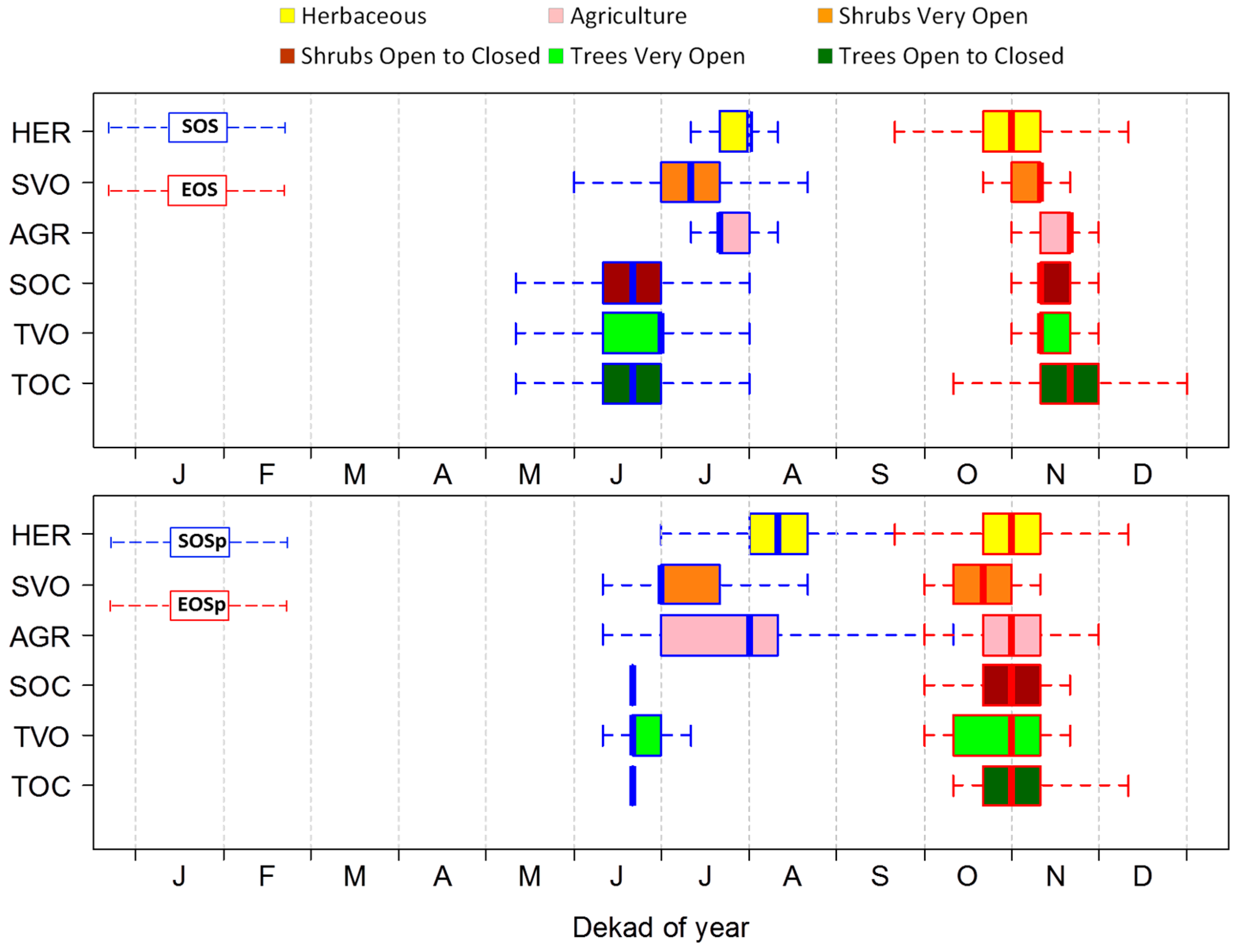
4.4. Comparison of FAPAR and Rainfall-Based Onset/End Metrics

The onset/end of the rainy season marks a vital time for livestock managers, pastoralists and stakeholders in natural resource management in West African regions [96]. Several definitions of the onset of the rainy season have been proposed in literature in relation to the local onset of persistent rainfall [97,98,99]. With advances in remote sensing technology, other metrics of onset/end dates have been proposed for assessing the plant growing season. These metrics are generally retrieved using specific rules based on thresholds of the amplitude of seasonal vegetation indices and on certain rainfall amounts over given time periods. So far as we know however, no study has yet investigated the relationship between the onset/end metrics derived from satellite vegetation indices and from rainfall estimates in the West African Sahel. We have shown the dissymmetry of the onset/end of the rainy season along the Sahel bioclimatic gradient, with the onset date staggered over 3 months from May in the south to July in the north. The end date is spread over only 1 month, from late September in the north to early November in the south, which corresponds with observations by [48]. Our results also show that FAPAR based on SOS occurred at the same time as rainfall based on SOSp across the whole study area, except for HER land cover class where SOS was observed one dekad earlier (see Table A2). There are many explanations for this. The onset of the growing season or greening of plants follows the rains, except for woody plants that start foliation earlier in response mainly to an increase in air temperature and humidity, enabling them to produce green leaves before the first rains [100,101,102]. In addition, herbaceous vegetation is sensitive to low rainfall amounts, requiring less than 25 mm for the first dekad and 20 mm for the following two dekads to trigger the growth. The thresholds set for calculating SOS and SOSp could therefore be adjusted to better match the region’s temporal dynamic. Apart from these botanical explanations, the reason could be related to data uncertainties. Almost no cloud-free optical satellite image is available at the start of season [59] and derived satellite data differ greatly from in situ measurements (e.g., NDVI) at this time [103]. Both the smoothing algorithm used for GEOV1 data (influenced by clouds) and the further smoothing via TIMESAT therefore add uncertainty to the FAPAR-based SOS calculation and our results indicate that this metric should be used with great caution at the annual scale.
Our results also showed that the onset dates of the rainy and growing seasons were more variable than their cessation, confirming the findings reported by [99]. The end date of both seasons occurs between late October and November for all land cover classes. The EOS is not entirely controlled by the end of the rains but depends also on the wilting of the herbaceous vegetation, which is determined by a biological clock (i.e., photoperiodicity) [15]. This was confirmed by our results where EOS dates, defined by the FAPAR reduction by 50% of the seasonal amplitude, occurred later than the cessation dates of the rainy season. The EOS delay is further influenced by crops that stay green longer, depending on their genetic features and soil tillage and by woody plants remaining green much longer, depending on their phenological behavior.

4.5. Early Assessment of Herbaceous Yield from Onset Metrics

For agricultural application, the SOS has attracted more attention from the scientific community and has been investigated in recent studies (i.e., [14,104,105]). It has frequently been used to investigate the land surface phenology trends in relation to climate variability [106]. After analyzing the SOS metrics against a proxy of biomass production in the Sahel however, [14] indicated that vegetation monitoring and biomass production forecasts should not be based on SOS in areas with non-significant correlation. Given that our study showed no significant relationship (at 0.05 p-level) between SOS and in situ herbaceous mass, this statement can be confirmed by our results and we do not recommend using this metric solely at the annual scale. The SOSp metrics however, were shown to have great potential for assessing herbaceous yield in the Sahelian region of Senegal. This was reflected in the VIAGRO-model where the SOSp variable was very important, confirming its superiority over SOS for detecting unfavorable rainfall conditions at the early stage of a growing season and therefore enabling early warnings of forthcoming risks of herbaceous mass deficits to be given to pastoral livestock managers and national stakeholders. Hence, even though the models presented here require a full season, this finding advances our knowledge towards an applicable early warning prediction [16].

5. Conclusions

Using the Fraction of Absorbed Photosynthetically Active Radiation (FAPAR) seasonal metrics computed with TIMESAT software and agrometeorological variables retrieved from the GeoWRSI program, we established three Cubist models for estimating herbaceous yield at the end of the season in the semi-arid areas of Senegal: (a) the VI-model with FAPAR metrics; (b) the AGRO-model with agrometeorological variables; and (c) the VIAGRO-model with both FAPAR and agrometeorological variables. All three models gave reasonable estimations of herbaceous yield over time and across land cover classes, among which those herbaceous areas with low woody cover showed the highest inter-annual variability and those in the south with higher woody cover showed lower variability over time. The VIAGRO-model gave the best estimation performance and indicated that the simultaneous use of agrometeorological data and FAPAR metrics improved the estimation accuracy and mitigated problems encountered with the sole use of FAPAR metrics (i.e., VI-model): (1) the saturation affecting optical remotely sensed vegetation data in areas of high vegetation productivity was attenuated; (2) the discrepancy between herbaceous mass and greenness (caused by species with high greenness and low mass production, or vice versa) was attenuated, with a weaker scattering around the low and high values closer to the 1:1 line (the additional use of agrometeorological data corrected for underestimations with the VI-model, particularly in sparsely vegetated areas); (3) the onset of the rainy season calculated from rainfall data was shown to be well suited for herbaceous mass assessment, in contrast to the onset of the growing season retrieved from FAPAR satellite data, which was not significantly related to herbaceous yields. Nevertheless, these metrics should be further investigated in order to improve our understanding of their temporal patterns and determine future setting parameters across Sahelian ecosystems.

Acknowledgments

This research was supported by the AGRICAB project (Contract No. 282621), funded by the European Union within the seventh Framework Programme (FP7) through the collaborative Work-Package 3.2 ‘Livestock Systems’ between the University of Liège (ULg, Arlon, Belgium) and the Centre de Suivi Ecologique (CSE, Dakar, Senegal). The research was also supported by the European Earth observation programme Copernicus Global Land, the GIOBIO (32-566) project and the Académie de Recherche et d’Enseignement Supérieur (ARES) in Belgium through the Centre pour le Partenariat et la Coopération au Développement (PACODEL) at the University of Liège. Martin Brandt received funding through the Marie Sklodowska-Curie grant (656564). The GeoWRSI software as well as rainfall and evapotranspiration data were obtained from the Famine Early Warning Systems Network (FEWS NET) data portal provided by USGS Earth Resources Observation and Science (EROS) Center for the FEWS NET Project. The authors wish to thank colleagues from the CSE, especially Abdoulaye Wélé, Aliou Diouf, Moussa Dramé, Moussa Sall, Aliou Ka, Gora Bèye and Ibrahima Diop, who helped to collect ground data from 2000 to 2015. Finally, we thank the three reviewers for their constructive comments and suggestions.

Author Contributions

Abdoul Aziz Diouf conceived the research, conducted the primary data analysis and drafted the manuscript. Bernard Tychon and Bakary Djaby advised on generating the research questions. Pierre Hiernaux and Martin Brandt contributed significantly to interpreting the results and reshaping the paper. Gayane Faye, Mouhamadou Bamba Diop and Jacques André Ndione reviewed the manuscript and offered comments and suggestions. Martin Brandt reviewed the paper and adjusted the language. All the authors contributed to writing the paper.

Conflicts of Interest

The authors declare no conflict of interest.

Appendix A

Table A1. Signification, unit and selection status after recursive feature elimination and variable inflation control of 17 agrometeorological variables provided by the GeoWRSI water balance model and used in the study. The 10 underlined variables correspond to those used for model development.
VariablesSignificationUnitSelection Status
WRSIWater requirement satisfaction index%No
SOSpStart of the rainy seasondekadYes
EOSpEnd of the rainy season-No
AETiActual evapotranspiration accumulated over the initial stage of the growing seasonmmNo
AETvActual evapotranspiration accumulated over the vegetative stage of the growing season-Yes
AETfActual evapotranspiration accumulated over the flowering stage of the growing season-Yes
AETrActual evapotranspiration accumulated over the ripening stage of the growing season-No
WDEFiWater deficit accumulated over the initial stage of the growing season-Yes
WDEFvWater deficit accumulated over the vegetative stage of the growing season-Yes
WDEFfWater deficit accumulated over the flowering stage of the growing season-Yes
WDEFrWater deficit accumulated over the ripening stage of the growing season-Yes
WSURiSurplus water accumulated over the initial stage of the growing season-No
WSURvSurplus water accumulated over the vegetative stage of the growing season-Yes
WSURfSurplus water accumulated over the flowering stage of the growing season-Yes
WSURrSurplus water accumulated over the ripening stage of the growing season-Yes
PPTcCumulated rainfall during the rainy season-No
PPTmAveraged rainfall during the rainy season-No
Table A2. Mean signed difference (in dekads) between onset metrics calculated from rainfall and FAPAR data across the agricultural and natural vegetation land cover classes in the study area.
Land Cover ClassesMean Signed Difference in Dekads
Start of SeasonEnd of Season
SOSp-SOSEOSp-EOS
Herbaceous1.30.1
Agriculture0.3−1.4
Shrubs very open0−2.1
Shrubs open to closed0−1.7
Trees very open0.3−1.6
Trees open to closed0.4−2.2
Overall mean0.4−1.5
Figure A1. Averaged (a) herbaceous, (b) woody leaf and (c) total plant yield of the 24 sites used in this study and their corresponding standard deviation (error bar) for the 2000–2015 period.
Remotesensing 08 00668 g012

References

  1. Anyamba, A.; Tucker, C.J. Analysis of sahelian vegetation dynamics using NOAA-AVHRR NDVI data from 1981–2003. J. Arid Environ. 2005, 63, 596–614. [Google Scholar] [CrossRef]
  2. Tagesson, T.; Fensholt, R.; Cropley, F.; Guiro, I.; Horion, S.; Ehammer, A.; Ardö, J. Dynamics in carbon exchange fluxes for a grazed semi-arid savanna ecosystem in West Africa. Agric. Ecosyst. Environ. 2015, 205, 15–24. [Google Scholar] [CrossRef]
  3. Carrière, M. Impact des Systèmes d’élevage Pastoraux sur L’environnement en Afrique et en asie Tropicale et Subtropicale Aride et Subaride; Technical Report; Scientific Environmental Monitoring Group—Universität des Saarlandes Institut für Biogeographie: Saarbrücken, Allemagne, 1996; p. 70. Available online: ftp://ftp.fao.org/docrep/nonfao/LEAD/x6215f/x6215F00.pdf (accessed on 23 March 2016).
  4. Tucker, C.J.; Vanpraet, C.; Boerwinkel, E.; Gaston, A. Satellite remote sensing of total dry matter production in the senegalese sahel. Remote Sens. Environ. 1983, 13, 461–474. [Google Scholar] [CrossRef]
  5. Tucker, C.J.; Vanpraet, C.L.; Sharman, M.J.; Itterstum, G.V. Satellite remote sensing of total herbaceous biomass production in the senegalese sahel: 1980–1984. Remote Sens. Environ. 1985, 17, 233–249. [Google Scholar] [CrossRef]
  6. Justice, C.O.; Hiernaux, P.H.Y. Monitoring the grasslands of the sahel using NOAA AVHRR data: Niger 1983. Int. J. Remote Sensi. 1986, 7, 1475–1497. [Google Scholar] [CrossRef]
  7. Seaquist, J.W.; Olsson, L.; Ardö, J. A remote sensing-based primary production model for grassland biomes. Ecol. Model. 2003, 169, 131–155. [Google Scholar] [CrossRef]
  8. Dardel, C.; Kergoat, L.; Hiernaux, P.; Mougin, E.; Grippa, M.; Tucker, C.J. Re-greening sahel: 30 years of remote sensing data and field observations (Mali, Niger). Remote Sens. Environ. 2014, 140, 350–364. [Google Scholar] [CrossRef]
  9. Tian, F.; Fensholt, R.; Verbesselt, J.; Grogan, K.; Horion, S.; Wang, Y. Evaluating temporal consistency of long-term global NDVI datasets for trend analysis. Remote Sens. Environ. 2015, 163, 326–340. [Google Scholar] [CrossRef]
  10. Baret, F.; Weiss, M.; Lacaze, R.; Camacho, F.; Makhmara, H.; Pacholcyzk, P.; Smets, B. Geov1: LAI and FAPAR essential climate variables and FCOVER global time series capitalizing over existing products. Part1: Principles of development and production. Remote Sens. Environ. 2013, 137, 299–309. [Google Scholar] [CrossRef]
  11. Prince, S.D. Satellite remote sensing of primary production: Comparison of results for sahelian grasslands 1981–1988. Int. J. Remote Sens. 1991, 12, 1301–1311. [Google Scholar] [CrossRef]
  12. Prince, S.D.; Goward, S.N. Global primary production: A remote sensing approach. J. Biogeogr. 1995, 22, 815–835. [Google Scholar] [CrossRef]
  13. Meroni, M.; Fasbender, D.; Kayitakire, F.; Pini, G.; Rembold, F.; Urbano, F.; Verstraete, M.M. Early detection of biomass production deficit hot-spots in semi-arid environment using FAPAR time series and a probabilistic approach. Remote Sens. Environ. 2014, 142, 57–68. [Google Scholar] [CrossRef]
  14. Meroni, M.; Rembold, F.; Verstraete, M.; Gommes, R.; Schucknecht, A.; Beye, G. Investigating the relationship between the inter-annual variability of satellite-derived vegetation phenology and a proxy of biomass production in the sahel. Remote Sens. 2014, 6, 5868–5884. [Google Scholar] [CrossRef] [Green Version]
  15. Brandt, M.; Hiernaux, P.; Tagesson, T.; Verger, A.; Rasmussen, K.; Diouf, A.A.; Mbow, C.; Mougin, E.; Fensholt, R. Woody plant cover estimation in drylands from earth observation based seasonal metrics. Remote Sens. Environ. 2016, 172, 28–38. [Google Scholar] [CrossRef]
  16. Diouf, A.; Brandt, M.; Verger, A.; Jarroudi, M.; Djaby, B.; Fensholt, R.; Ndione, J.; Tychon, B. Fodder biomass monitoring in sahelian rangelands using phenological metrics from FAPAR time series. Remote Sens. 2015, 7, 9122–9148. [Google Scholar] [CrossRef]
  17. Funk, C.C.; Brown, M.E. Intra-seasonal NDVI change projections in semi-arid Africa. Remote Sens. Environ. 2006, 101, 249–256. [Google Scholar] [CrossRef]
  18. Cornet, A. Utilisation de modéles simples de bilan hydrique et de production de biomasse pour déterminer les potentialités de production de parcours en zone sahélienne sénégalaise. In Proceedings of the Workshop on Land Evaluation for Extensive Grazing, Wageningen, The Netherlands, 31 October–4 November 1984; pp. 207–228.
  19. Hickler, T.; Eklundh, L.; Seaquist, J.W.; Smith, B.; Ardö, J.; Olsson, L.; Sykes, M.T.; Sjöström, M. Precipitation controls sahel greening trend. Geophys. Res. Lett. 2005, 32, L21415. [Google Scholar] [CrossRef]
  20. Ali, A. Variabilité et changements du climat au sahel : Ce que l’observation nous apprend sur la situation actuelle. Grain de sel 2010, 49, 13–14. [Google Scholar]
  21. Huber, S.; Fensholt, R. Analysis of teleconnections between AVHRR-based sea surface temperature and vegetation productivity in the semi-arid sahel. Remote Sens. Environ. 2011, 115, 3276–3285. [Google Scholar] [CrossRef]
  22. Brandt, M.; Mbow, C.; Diouf, A.A.; Verger, A.; Samimi, C.; Fensholt, R. Ground and satellite based evidence of the biophysical mechanisms behind the greening sahel. Glob. Chang. Biol. 2015, 1610–1620. [Google Scholar] [CrossRef] [PubMed]
  23. Ibrahim, Y.; Balzter, H.; Kaduk, J.; Tucker, C. Land degradation assessment using residual trend analysis of Gimms NDVI3g, soil moisture and rainfall in sub-saharan West Africa from 1982 to 2012. Remote Sens. 2015, 7, 5471–5494. [Google Scholar] [CrossRef]
  24. Penning de Vries, F.W.T.; Djitèye, M.A. La Productivité des Pâturages Sahéliens: Une Étude des Sols, des Végétations et de L’exploitation de Cette Ressource Naturelle; Centre for Agricultural Publishing and Documentation: Wageningen, The Netherlands, 1982; p. 525. [Google Scholar]
  25. Breman, H.; De Ridder, N. Manuel Sur Les Pâturages des Pays Sahéliens; CTA: Wageningen, The Netherlands, 1991; p. 481. [Google Scholar]
  26. Tarnavsky, E.; Grimes, D.; Maidment, R.; Black, E.; Allan, R.; Stringer, M.; Chadwick, R.; Kayitakire, F. Extension of the tamsat satellite-based rainfall monitoring over Africa and from 1983 to present. J. Appl. Meteorol. Climatol. 2014, 53, 2805–2822. [Google Scholar] [CrossRef]
  27. Xie, P.; Arkin, P.A. Analysis of global monthly precipitation using gauge observations, satellite estimates, and numerical model prediction. J. Clim. 1996, 9, 840–858. [Google Scholar] [CrossRef]
  28. Novella, N.S.; Thiaw, W.M. African rainfall climatology version 2 for famine early warning systems. J. Appl. Meteorol. Climatol. 2013, 52, 588–606. [Google Scholar] [CrossRef]
  29. Hiernaux, P. Distribution des pluies et production herbacée au sahel:Une méthode empirique pour caractériser la distribution des précipitations journalières et ses effets sur la production herbacée. In Premiers Résultats Acquis Dans le Sahel Malien; Doc. Prog. N AZ 98; CIPEA: Bamako, Mali, 1983. [Google Scholar]
  30. CSE. Rapport sur l’état de l’environnement au sénégal; Centre de Suivi Ecologique: Dakar, Senegal, 2010; p. 266. [Google Scholar]
  31. Breshears, D.; Barnes, F. Interrelationships between plant functional types and soil moisture heterogeneity for semiarid landscapes within the grassland/forest continuum: A unified conceptual model. Landsc. Ecol. 1999, 14, 465–478. [Google Scholar] [CrossRef]
  32. Hiernaux, P.; Ayantunde, A.; Kalilou, A.; Mougin, E.; Gérard, B.; Baup, F.; Grippa, M.; Djaby, B. Trends in productivity of crops, fallow and rangelands in southwest niger: Impact of land use, management and variable rainfall. J. Hydrol. 2009, 375, 65–77. [Google Scholar]
  33. Hiernaux, P.; Mougin, E.; Diarra, L.; Soumaguel, N.; Lavenu, F.; Tracol, Y.; Diawara, M. Sahelian rangeland response to changes in rainfall over two decades in the Gourma region, Mali. J. Hydrol. 2009, 375, 114–127. [Google Scholar]
  34. Rojas, O.; Rembold, F.; Royer, A.; Negre, T. Real-time agrometeorological crop yield monitoring in Eastern Africa. Agron. Sustain. Dev. 2005, 25, 63–77. [Google Scholar]
  35. Doorenbos, J.; Pruitt, W.O. Guidelines for Predicting Crop Water Requirements; FAO Irrigation and Drainage paper No. 24; FAO: Rome, Italy, 1977. [Google Scholar]
  36. Frère, M.; Popov, G. Agrometeorological Crop Monitoring and Forecasting; FAO plant production and protection paper No. 17.; FAO: Rome, Italy, 1979. [Google Scholar]
  37. Verdin, J.; Klaver, R. Grid cell based crop water accounting for the famine early warning system. Hydrol. Proces. 2002, 16, 617–1630. [Google Scholar]
  38. Senay, G.B.; Verdin, J. Evaluating the performance of a crop water balance model in estimating regional crop production. In Proceedings of the Pecora 15/Land Satellite Information IV/ISPRS Commission I/FIEOS 2002 Conference, Denver, CO, USA, 10–15 November 2002.
  39. Senay, G.B.; Verdin, J.P.; Rowland, J. Developing an operational rangeland water requirement satisfaction index. Int.J. Remote Sens. 2011, 32, 6047–6053. [Google Scholar]
  40. Mougin, E.; Lo Seena, D.; Rambal, S.; Gaston, A.; Hiernaux, P. A regional sahelian grassland model to be coupled with multispectral satellite data. I: Model description and validation. Remote Sens. Environ. 1995, 52, 181–193. [Google Scholar] [CrossRef]
  41. Rudorff, B.F.T.; Batista, G.T. Yield estimation of sugarcane based on agrometeorological-spectral models. Remote Sens. Environ. 1990, 33, 183–192. [Google Scholar] [CrossRef]
  42. Stancioff, A.; Staljanssens, M.; Tappan, G. Mapping and Remote Sensing of the Resources of the Republic of Senegal: A study of the Geology, Hydrology, Soils, Vegetation and Land use Potential; SDSU-RSI-86-01; Remote Sensing Institute of South Dakota State University: Brookings, SD, USA, 1986. [Google Scholar]
  43. Herman, A.; Kumar, V.B.; Arkin, P.A.; Ko Usky, J.V. Objectively determined 10-day african rainfall estimates created for famine early warning systems. Int. J. Remote Sens. 1997, 18, 2147–2159. [Google Scholar] [CrossRef]
  44. Xie, P.; Arkin, P.A. A 17-year monthly analysis based on gauge observations, satellite estimates, and numerical model outputs. Bull. Am. Meteorol. Soc. 1997, 78, 2539–2558. [Google Scholar] [CrossRef]
  45. Maignen, R. Notice explicative, carte pédologique du sénégal au 1/1.000.000; Publication ORSTOM: Dakar, Sénégal, 1965. [Google Scholar]
  46. Tappan, G.G.; Sall, M.; Wood, E.C.; Cushing, M. Ecoregions and land cover trends in senegal. J. Arid Environ. 2004, 59, 427–462. [Google Scholar] [CrossRef]
  47. Valenza, J. Dynamisme de quelques types de pâturages naturels sahélo-soudaniens en république du sénégal. In Proceedings of the XIIIe International Grassland Congress, Leipzig, Allemagne, 18–27 May 1977.
  48. Hiernaux, P.; Le Houérou, H.N. Les parcours du sahel. Sécheresse 2006, 17, 51–71. [Google Scholar]
  49. CSE. Suivi de la Production Végétale 2013 au Sénégal; National Report; Centre de Suivi Ecologique of Dakar: Dakar, Senegal, 2013. [Google Scholar]
  50. CSE. Suivi de la Production Végétale 2014 au Sénégal; National Report; Centre de Suivi Ecologique of Dakar: Dakar, Senegal, 2014. [Google Scholar]
  51. FAO. Global Land Cover Network: Senegal Land Cover Mapping. Available online: http://www.Glcn.Org/databases/se_landcover_en.Jsp (accessed on 2 November 2015).
  52. FAO. Land Cover Changes: Senegal 1990–2005. 2009. Available online: http://www.glcn.org/downs/prj/senegal/Sen_lc_change_report_dec08.pdf (accessed on 2 November 2015).
  53. FAO. Senegal Land Cover Mapping. 2009. Available online: http://www.glcn.org/downs/prj/senegal/Sen_lc_report_dec08.pdf (accessed on 27 August 2015).
  54. FAO. Senegal Land Cover Classes Description. 2009. Available online: http://www.glcn.org/downs/prj/senegal/Sen_lc_classes_descr_dec08.pdf (accessed on 2 November 2015).
  55. Diouf, A.; Sall, M.; Wélé, A.; Dramé, M. Méthode d’échantillonnage de la production primaire sur le terrain; Document technique; Centre de suivi écologique de Dakar: Dakar, Sénégal, 1998. [Google Scholar]
  56. Verger, A.; Baret, F.; Weiss, M.; Filella, I.; Peñuelas, J. Geoclim: A global climatology of LAI, FAPAR, and FCOVER from vegetation observations for 1999–2010. Remote Sens. Environ. 2015. [Google Scholar] [CrossRef]
  57. Jönsson, P.; Eklundh, L. Timesat—A program for analyzing time-series of satellite sensor data. Comput. Geosci. 2004, 30, 833–845. [Google Scholar] [CrossRef]
  58. Chen, J.; Jönsson, P.; Tamura, M.; Gu, Z.; Matsushita, B.; Eklundh, L. A simple method for reconstructing a high-quality NDVI time-series data set based on the Savitzky–Golay filter. Remote Sens. Environ. 2004, 91, 332–344. [Google Scholar] [CrossRef]
  59. Fensholt, R.; Anyamba, A.; Stisen, S.; Sandholt, I.; Pak, E.; Small, J. Comparisons of compositing period length for vegetation index data from polar-orbiting and geostationary satellites for the cloud-prone region of West Africa. Photogramm. Eng. Remote Sens. 2007, 73, 297–309. [Google Scholar] [CrossRef]
  60. Senay, G. Crop Water Requirement Satisfaction Index (WRSI): Model Description. 2004. Available online: http://iridl.ldeo.columbia.edu/documentation/usgs/adds/wrsi/WRSI_readme.pdf (accessed on 17 July 2015).
  61. Senay, G.B.; Verdin, J. Characterization of yield reduction in ethiopia using a GIS-based crop water balance model. Can. J. Remote Sens. 2003, 29, 687–692. [Google Scholar] [CrossRef]
  62. Senay, G.B.; Verdin, J. Using a GIS-based water balance model to assess regional crop performance. In Proceedings of the Fifth International Workshop on Application of Remote Sensing in Hydrology, Montpellier, France, 2–5 October 2001.
  63. Senay, G. Modeling landscape evapotranspiration by integrating land surface phenology and a water balance algorithm. Algorithms 2008, 1, 52–68. [Google Scholar] [CrossRef]
  64. Shuttleworth, J. Evaporation. In Handbook of Hydrology; Maidment, D., Ed.; McGraw-Hill: New York, NY, USA, 1992; pp. 1–4. [Google Scholar]
  65. Climate Hazard Group. Rainfall Estimate and Potential Evapotranspiration Data. Available online: Ftp://ftp.Chg.Ucsb.Edu/pub/org/chg/products/geowrsi/archives/ (accessed on 18 December 2015).
  66. FEWS NET. Fews Data Downloads. Available online: Http://earlywarning.Usgs.Gov/fews/datadownloads (accessed on 18 december 2015).
  67. FAO. Digital Soil Map of the World (CDROM); Food and Agriculture Organization of the United Nations: Rome, Italy, 1994. [Google Scholar]
  68. Allen, R.G.; Pereira, L.S.; Raes, D.; Smith, M. Crop Evapotranspiration; FAO Irrigation and Drainage Paper No. 56; FAO: Rome, Italy, 1998. [Google Scholar]
  69. AGRHYMET. Méthodologie de suivi des zones à risque. In Agrhymet flash, bulletin de suivi de la campagne agricole au sahel 0/96; AGRHYMET: Niamey, Niger, 1996; Volume 2, pp. 1–2. [Google Scholar]
  70. Domingos, P. A few useful things to know about machine learning. Commun. ACM 2012, 55, 78–87. [Google Scholar] [CrossRef]
  71. De Benedetto, D.; Castrignanò, A.; Quarto, R. A geostatistical approach to estimate soil moisture as a function of geophysical data and soil attributes. Proc. Environ. Sci. 2013, 19, 436–445. [Google Scholar] [CrossRef]
  72. Fraser, R.H.; Li, Z. Estimating fire-related parameters in boreal forest using spot vegetation. Remote Sens. Environ. 2002, 82, 95–110. [Google Scholar] [CrossRef]
  73. Zhang, C.; Kovacs, J.; Liu, Y.; Flores-Verdugo, F.; Flores-de-Santiago, F. Separating mangrove species and conditions using laboratory hyperspectral data: A case study of a degraded mangrove forest of the mexican pacific. Remote Sens. 2014, 6, 11673–11688. [Google Scholar] [CrossRef]
  74. Hastie, T.; Tibshirani, R.; Friedman, J. The Elements of Statistical Learning: Data Mining, Inference, and Prediction; Springer-Verlag: New York, NY, USA, 2009. [Google Scholar]
  75. Kuhn, M.; Johnson, K. Applied Predictive Modeling; Springer: New York, NY, USA, 2013. [Google Scholar]
  76. Guyon, I.; Weston, J.; Barnhill, S.; Vapnik, V. Gene selection for cancer classification using support vector machines. Mach. Learn. 2002, 46, 389–422. [Google Scholar] [CrossRef]
  77. Marill, T.; Green, D.M. On the effectiveness of receptors in recognition systems. IEEE Trans. Inf. Theory 1963, 9, 11–17. [Google Scholar] [CrossRef]
  78. Kuhn, M.; Wing, J.; Weston, S.; Williams, A.; Keefer, C.; Engelhardt, A.; Cooper, T.; Mayer, Z.; The R Core Team. Caret: Classification and Regression Training, R Package Version 6.0–24. Available online: Http://cran.R-project.Org/package=caret (accessed on 25 June 2015).
  79. Liaw, A.; Wiener, M. Classification and regression by randomforest. R News 2002, 2, 18–22. [Google Scholar]
  80. Belsley, D.A.; Kuh, E.; Welsh, R.E. Regression Diagnostics: Identifying Influential Data and Sources of Collinearity; John Wiley & Sons: New York, NY, USA, 1980. [Google Scholar]
  81. Herrmann, S.; Wickhorst, A.; Marsh, S. Estimation of tree cover in an agricultural parkland of senegal using rule-based regression tree modeling. Remote. Sens. 2013, 5, 4900–4918. [Google Scholar] [CrossRef]
  82. Brosofske, K.D.; Froese, R.E.; Falkowski, M.J.; Banskota, A. A review of methods for mapping and prediction of inventory attributes for operational forest management. For. Sci. 2014, 60, 733–756. [Google Scholar] [CrossRef]
  83. White, A.B.; Kumar, P.; Tcheng, D. A data mining approach for understanding topographic control on climate-induced inter-annual vegetation variability over the united states. Remote Sens. Environ. 2005, 98, 1–20. [Google Scholar] [CrossRef]
  84. Kuhn, M.; Weston, S.; Keefer, C.; Coulter, N. Cubist Models for Regression. 2012. Available online: http://cran.r-project.org/web/packages/Cubist/vignettes/cubist.pdf (accessed on 25 June 2015).
  85. Kohavi, R. A study of cross-validation and bootstrap for accuracy estimation and model selection. Int. J. Conf. Artif. Int. 1995, 14, 1137–1145. [Google Scholar]
  86. Refaeilzadeh, P.; Tang, L.; Liu, H. Cross-validation. In Encyclopedia of Database Systems; Liu, L., ÖZsu, M.T., Eds.; Springer: Heidelberg, Germany, 2009; pp. 532–538. [Google Scholar]
  87. Jin, Y.; Yang, X.; Qiu, J.; Li, J.; Gao, T.; Wu, Q.; Zhao, F.; Ma, H.; Yu, H.; Xu, B. Remote sensing-based biomass estimation and its spatio-temporal variations in temperate grassland, Northern China. Remote Sens. 2014, 6, 1496–1513. [Google Scholar] [CrossRef]
  88. Tian, F.; Brandt, M.; Liu, Y.Y.; Verger, A.; Tagesson, T.; Diouf, A.A.; Rasmussen, K.; Mbow, C.; Wang, Y.; Fensholt, R. Remote sensing of vegetation dynamics in drylands: Evaluating vegetation optical depth (VOD) using AVHRR NDVI and in situ green biomass data over west African Sahel. Remote Sens. Environ. 2016, 177, 265–276. [Google Scholar] [CrossRef]
  89. Diouf, A.A.; Djaby, B.; Diop, M.B.; Wele, A.; Ndione, J.-A.; Tychon, B. Fonctions d’ajustement pour l’estimation de la production fourragère herbacée des parcours naturels du sénégal à partir du ndvi s10 de spot-vegetation. In Proceedings of the XXVIIe Colloq. de l’Asso. Int. de Climatol, Dijon, France, 2–5 July 2014; pp. 284–289.
  90. Xiaoping, W.; Ni, G.; Kai, Z.; Jing, W. Hyperspectral remote sensing estimation models of aboveground biomass in gannan rangelands. Proc. Environ. Sci. 2011, 10, 697–702. [Google Scholar] [CrossRef]
  91. Santin-Janin, H.; Garel, M.; Chapuis, J.L.; Pontier, D. Assessing the performance of NDVI as a proxy for plant biomass using non-linear models: A case study on the kerguelen archipelago. Polar Biol. 2009, 32, 861–871. [Google Scholar] [CrossRef]
  92. Huete, A.; Didan, K.; Miura, T.; Rodriguez, E.P.; Gao, X.; Ferreira, L.G. Overview of the radiometric and biophysical performance of the modis vegetation indices. Remote Sens. Environ. 2002, 83, 195–213. [Google Scholar] [CrossRef]
  93. Touré, I.; Ickowicz, A.; Wane, A.; Garba, I.; Gerber, P.; Atté, I.; Cesaro, J.D.; Diop, A.T.; Djibo, S.; Ham, F.; et al. Atlas of Trends in Pastoral Systems in Sahel; FAO and CIRAD: Montpellier, France, 2012. [Google Scholar]
  94. Ikegami, M.; Barrett, C.B.; Chantarat, S. Dynamic effects of index based livestock insurance on household intertemporal behavior and welfare. In Proceedings of the Research Conference on Microinsurance, Twente, The Netherlands, 11–12 April 2012.
  95. Chantarat, S.; Mude, A.G.; Barrett, C.B.; Carter, M.R. Designing index based livestock insurance for managing asset risk in Nothern Kenya. J. Risk Insur. 2013, 80, 205–237. [Google Scholar] [CrossRef]
  96. Fitzpatrick, R.G.J.; Bain, C.L.; Knippertz, P.; Marsham, J.H.; Parker, D.J. The West African monsoon onset: A concise comparison of definitions. J. Clim. 2015, 28, 8673–8694. [Google Scholar] [CrossRef]
  97. Marteau, R.; Moron, V.; Philippon, N. Spatial coherence of monsoon onset over western and central sahel (1950–2000). J. Clim. 2009, 22, 1313–1324. [Google Scholar] [CrossRef]
  98. Omotosho, J.B.; Balogun, A.A.; Ogunjobi, K. Predicting monthly and seasonal rainfall, onset and cessation of the rainy season in west africa using only surface data. Int. J. Climatol. 2000, 20, 865–880. [Google Scholar] [CrossRef]
  99. Sivakumar, M.V.K. Predicting rainy season potential from the onset of rains in southern sahelian and sudanian climatic zones of West Africa. Agric. For. Meteorol. 1988, 42, 295–305. [Google Scholar] [CrossRef]
  100. Ali, M.; Saadou, M.; Jean, L. Phénologie de quelques espèces ligneuses du parc national du «W» (Niger). Science et Changements Planétaires/Sécheresse 2007, 18, 354–358. [Google Scholar]
  101. Devineau, J.-L. Seasonal rhythms and phenological plasticity of savanna woody species in a fallow farming system (South-West Burkina Faso). J. Trop. Ecol. 1999, 15, 497–513. [Google Scholar] [CrossRef]
  102. Hiernaux, P.H.Y.; Cissé, M.I.; Diarra, L.; De Leeuw, P.N. Fluctuations saisonnières de la feuillaison des arbres et des buissons sahéliens. Conséquences pour la quantification des ressources fourragères. Revue D’élevage et de Médecine Vétérinaire des Pays Tropicaux 1994, 47, 117–125. [Google Scholar]
  103. Proud, S.R.; Zhang, Q.; Schaaf, C.; Fensholt, R.; Rasmussen, M.O.; Shisanya, C.; Mutero, W.; Mbow, C.; Anyamba, A.; Pak, E.; et al. The normalization of surface anisotropy effects present in seviri reflectances by using the modis brdf method. IEEE Tran. Geosci. Remote Sens. 2014, 52, 6026–6039. [Google Scholar] [CrossRef]
  104. Mbow, C.; Fensholt, R.; Rasmussen, K.; Diop, D. Can vegetation productivity be derived from greenness in a semi-arid environment? Evidence from ground-based measurements. J. Arid Environ. 2013, 97, 56–65. [Google Scholar] [CrossRef]
  105. Vintrou, E.; Bégué, A.; Baron, C.; Saad, A.; Lo Seen, D.; Traoré, S. A comparative study on satellite and model-based crop phenology in West Africa. Remote Sens. 2014, 6, 1367–1389. [Google Scholar] [CrossRef] [Green Version]
  106. Begue, A.; Vintrou, E.; Saad, A.; Hiernaux, P. Differences between cropland and rangeland MODIS phenology (start-of-season) in Mali. Int. J. Appl. Earth Obs. Geoinf. 2014, 31, 167–170. [Google Scholar] [CrossRef]
Figure 1. Location of the monitoring sites and the main land cover classes [51]. The sites are identified by their position in a grid where Cx indicates the column number and Ly corresponds to the line number with x and y varying between 1 and 9. The isohyets are based on average rainfall estimates provided by FEWS NET between 2000 and 2015 [44].
Remotesensing 08 00668 g001
Figure 2. Seasonal FAPAR metrics considered in this study and shown for a single pixel. The base value (BVAL) represents the averaged minimum values over the annual cycle (i.e., before and after the growing season).
Remotesensing 08 00668 g002
Figure 3. Overall crop coefficient curve for Senegal’s Sahelian rangelands during a growing season of 90 days. The growing period was divided into four phases: initial (i); vegetative (v); flowering (f); ripening (r). SOSp indicates the mean date of the onset of the rainy season in the 2000-2015 period. Numbers in brackets indicate the total days of the phase.
Remotesensing 08 00668 g003
Figure 4. Workflow for the development of the rule-based piecewise regression (i.e., Cubist) models for herbaceous yield estimation.
Remotesensing 08 00668 g004
Figure 5. Importance of the predictor variables for the three herbaceous yield estimation models: (a) VI-model; (b) AGRO-model; (c) VIAGRO-model. Single variable importance initially given as the means of the percentage of use in model conditions and equations were then normalized to sum 100% for each model.
Remotesensing 08 00668 g005
Figure 6. Accuracy assessment of the developed Cubist models: relationship between observed and predicted herbaceous yield for; (a) the VI-model; (b) the AGRO-model; (c) the VIAGRO-model.
Remotesensing 08 00668 g006
Figure 7. Latitudinal variation of the herbaceous yield estimated by the: (a) VI-model; (b) AGRO-model; (c) VIAGRO-model during the 2000–2015 period.
Remotesensing 08 00668 g007
Figure 8. Coefficients of variation in annual herbaceous yield estimated by the three models: (a) VI-model; (b) AGRO-model; (c) VIAGRO-model, according to the 2000–2015 average.
Remotesensing 08 00668 g008
Figure 9. Inter-annual variations in rainfall and estimated herbaceous yield over the whole study area from the: (a) VI-model; (b) AGRO-model; (c) VIAGRO-model. Rainfall values were averaged from the 24 monitoring sites and the estimated herbaceous yield was averaged from all pixels covered by a given class. Colors and acronyms are explained in Figure 8 and Table 1.
Remotesensing 08 00668 g009
Figure 10. Boxplots of the start and end of season metrics derived from FAPAR (SOS and EOS) and rainfall data (SOSp and EOSp), averaged over the 2000–2015 period for each land cover class.
Remotesensing 08 00668 g010
Figure 11. Relationship between anomalies of herbaceous yield mass and onset of: (a) the growing season (SOS); (b) the rainy season (SOSp) for the whole studied area; (c) for each land cover class. Numbers on bars correspond to p-values.
Remotesensing 08 00668 g011
Table 1. General Descriptions of Land Cover Classes [53,54]. Woody Cover Values were obtained from the Woody Cover Map Provided by [15] and Correspond to the Averaged Values of Pixels Covered by Classes.
Land Cover ClassAbbreviationShort DescriptionArea (km²)Area (%)Woody Cover (%)Number of Sites
HerbaceousHEROpen to closed herbaceous vegetation with sparse trees and shrubs38,04330.53913
Shrubs very openSVOVery open shrubs33,72427.07178
Shrubs open to closedSOCOpen to closed shrubs12,1559.75282
Trees very openTVOVery open trees, gallery forest88897.13251
Trees open to closedTOCOpen to closed trees, gallery forest92747.44250
AgricultureAGRLarge to small tree plantations and rainfed herbaceous crops19,48315.64140
Other classes-Bare areas, urban areas and water bodies30412.44-0
Generic height classification: herbaceous = 0.03 to 3 m; shrubs = 0.3 to 5 m; trees = 3 to 30 m.

