
Landscape Effects of Wildfire on Permafrost Distribution in Interior Alaska Derived from Remote Sensing

 ,
, 
Abstract
:
1. Introduction
2. Materials and Methods
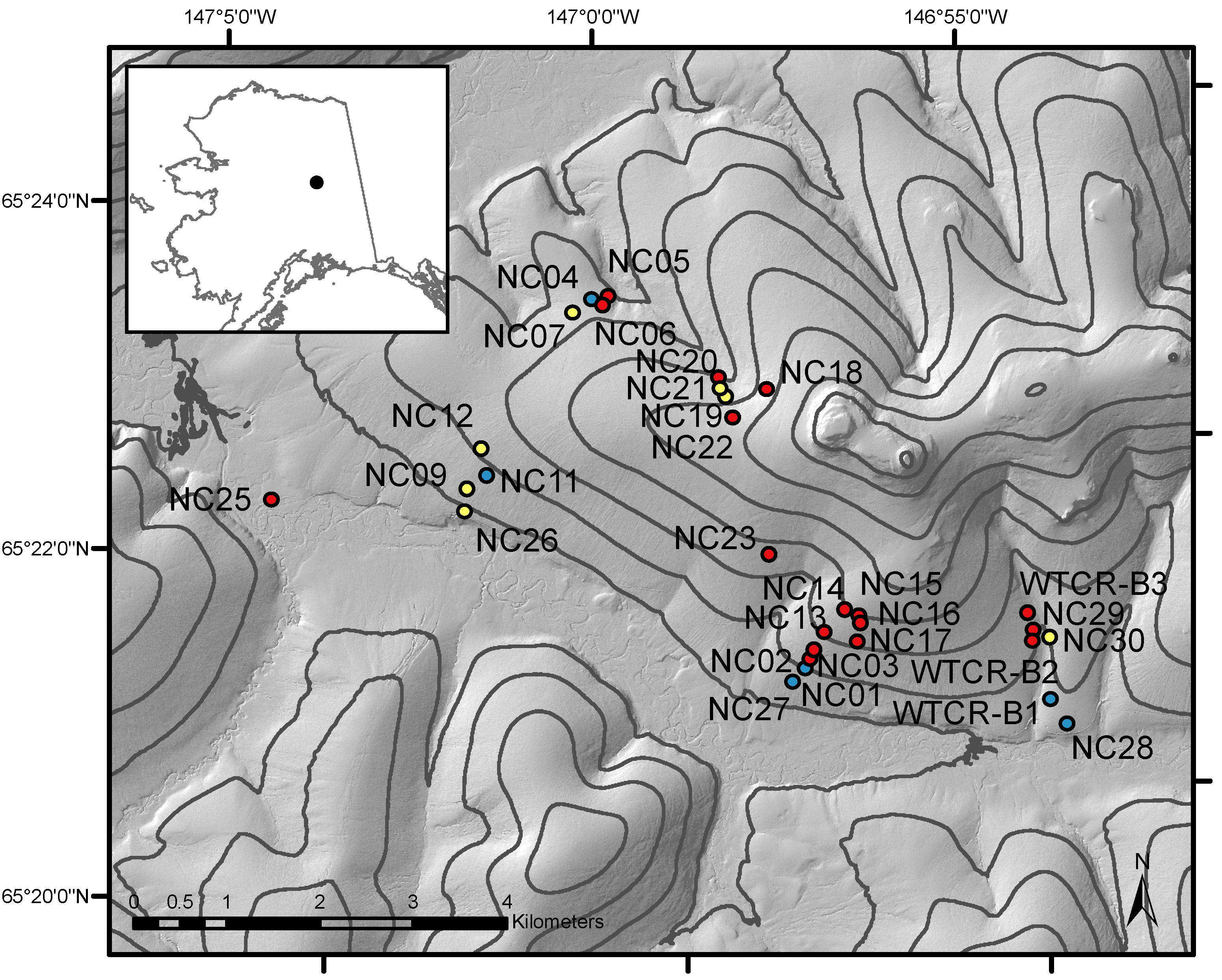
2.1. Study Area and Design
2.2. Vegetation Sampling
2.3. Soil Sampling
2.4. Remote Sensing
2.4.1. LiDAR
2.4.2. Radar
2.4.3. Landsat
2.5. Data Analysis
2.5.1. Vegetation
2.5.2. Soils
2.5.3. Remote Sensing
2.5.4. Mapping
3. Results
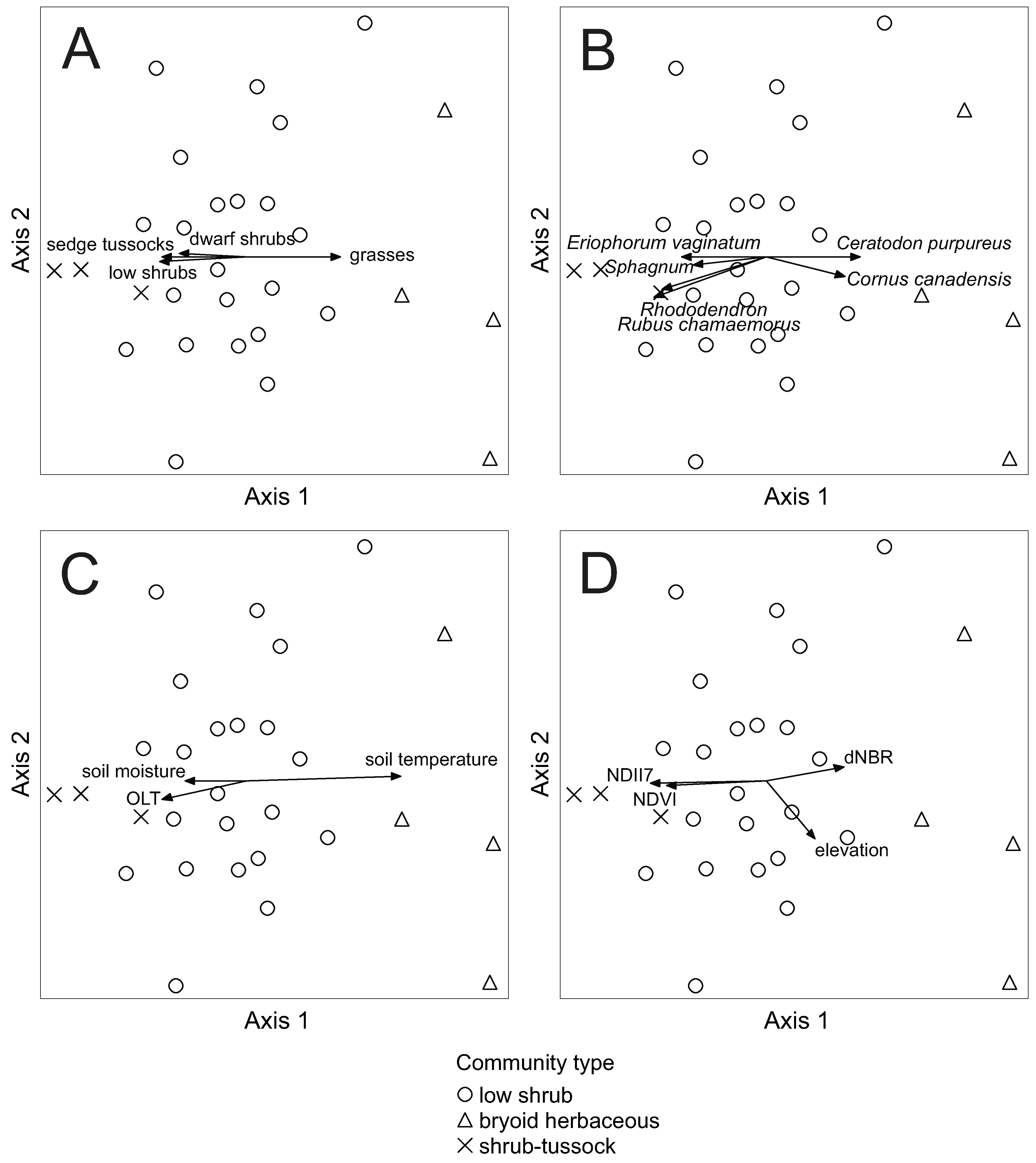
3.1. Vegetation
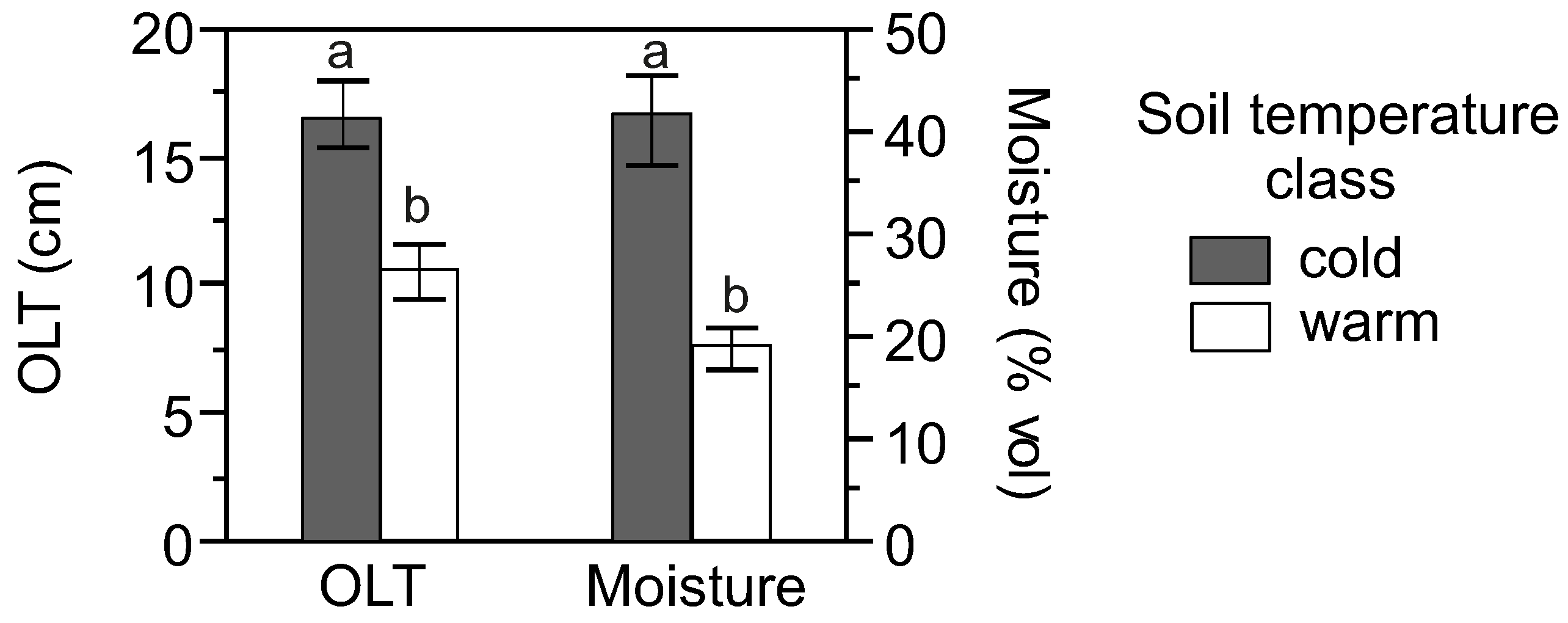
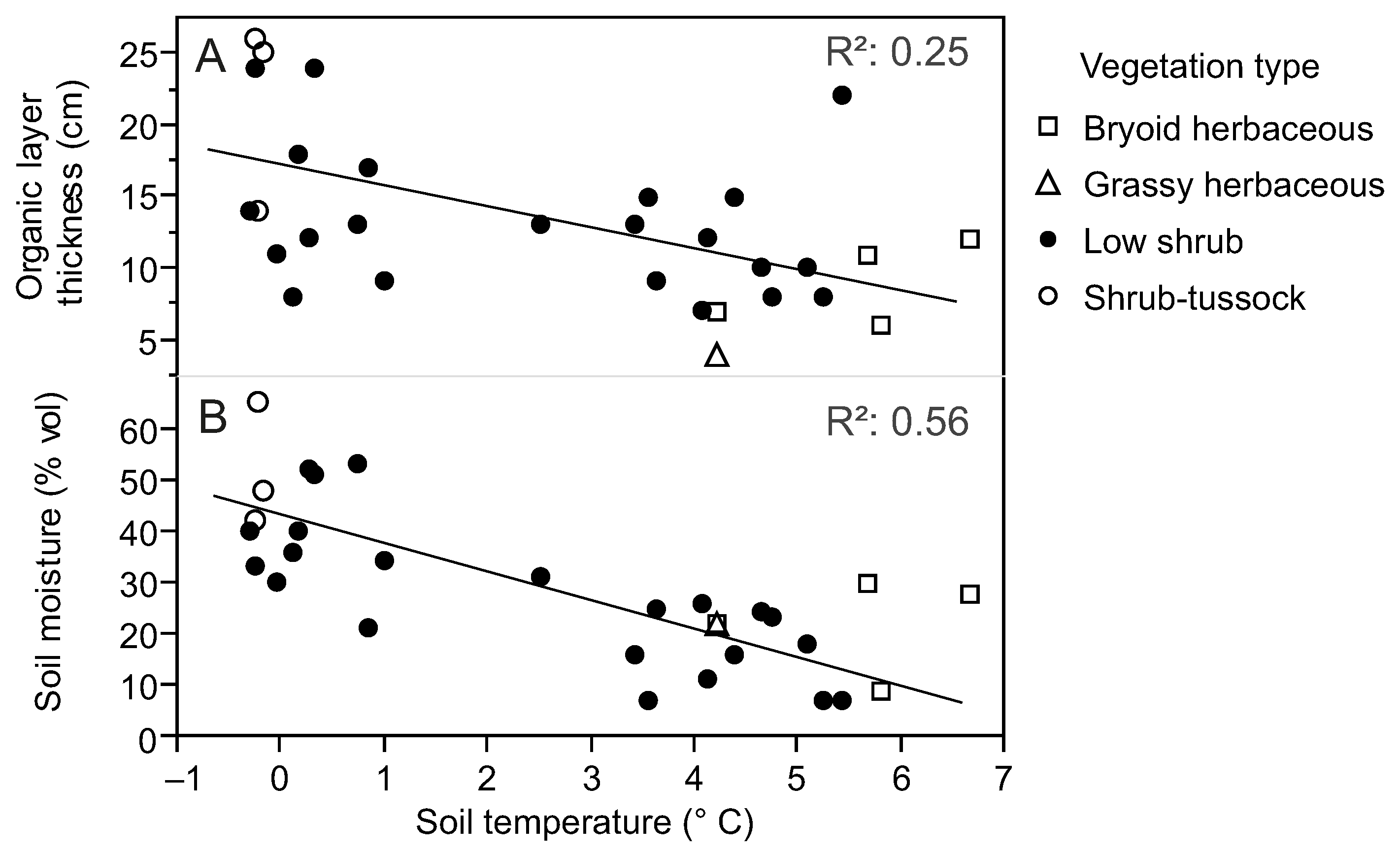
3.2. Soils
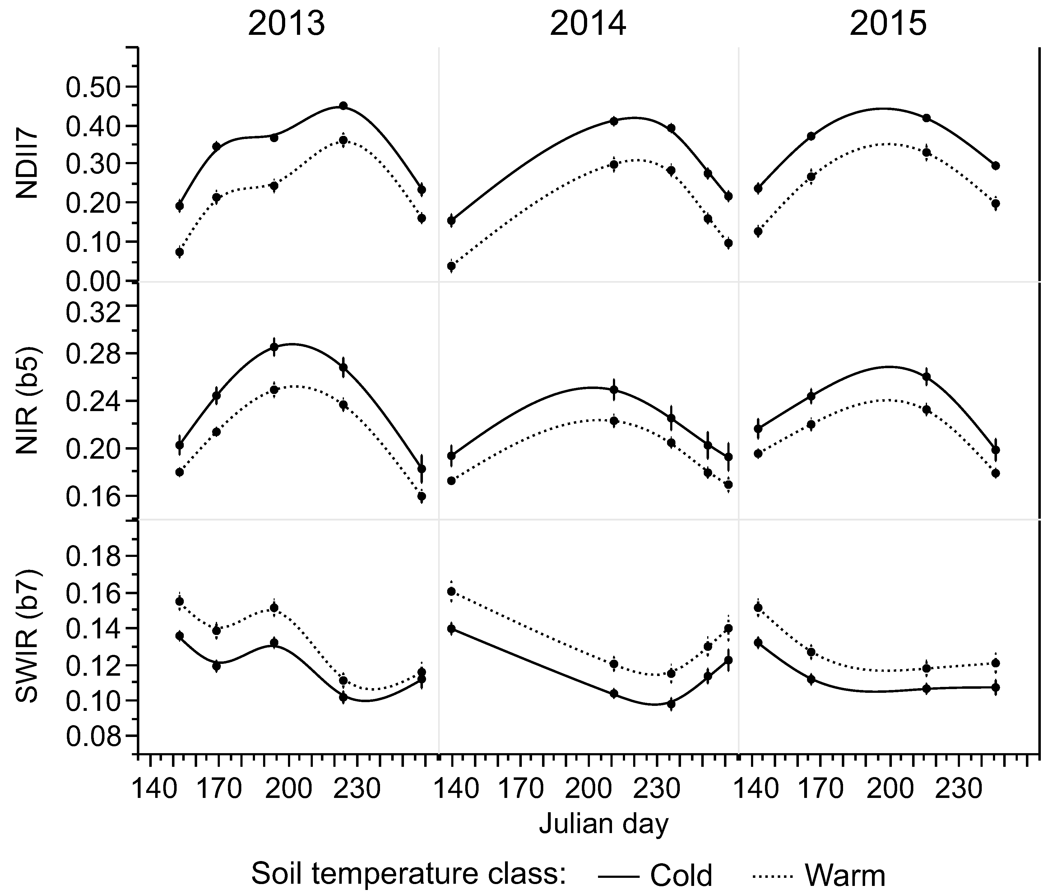
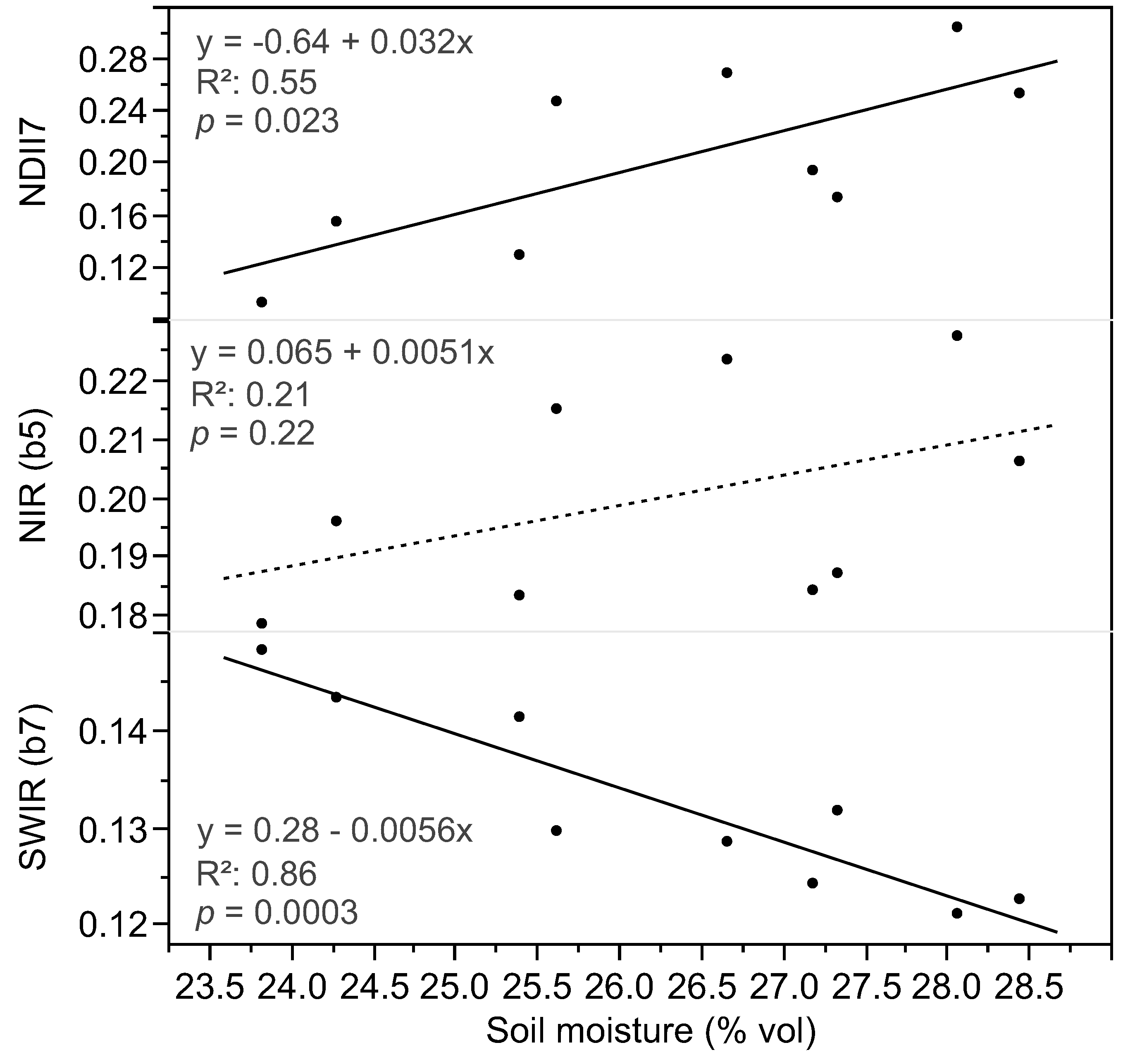
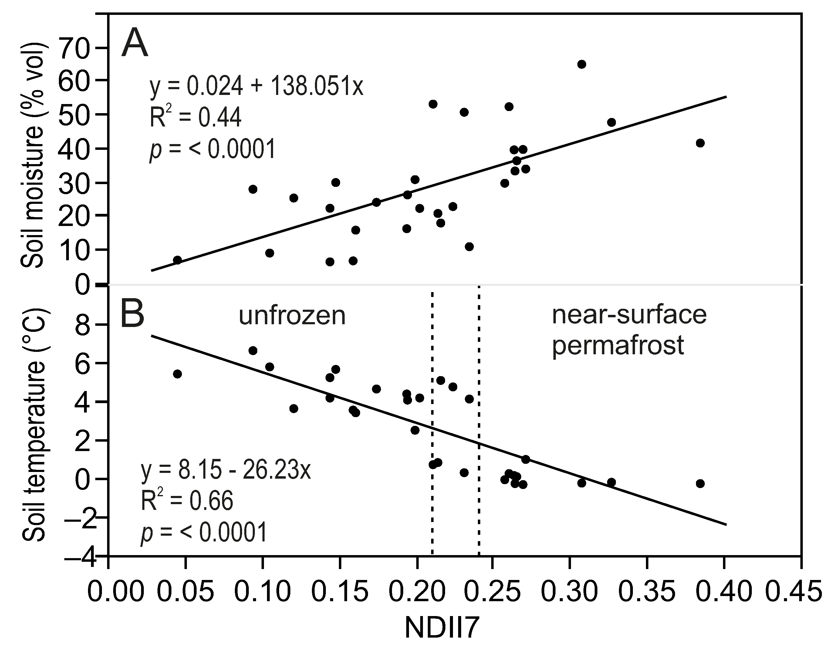
3.3. Remote Sensing
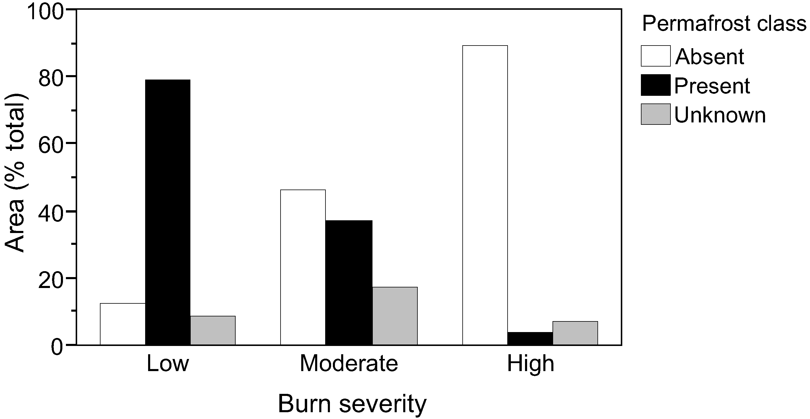
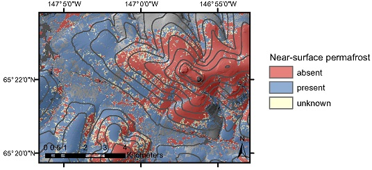
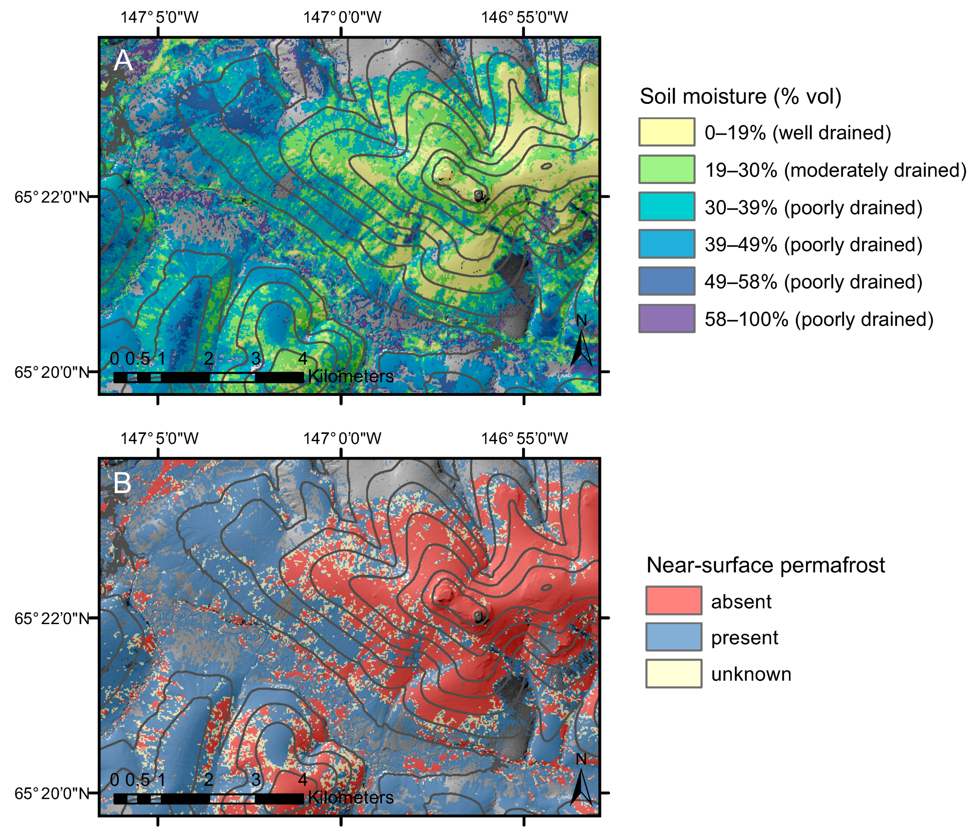
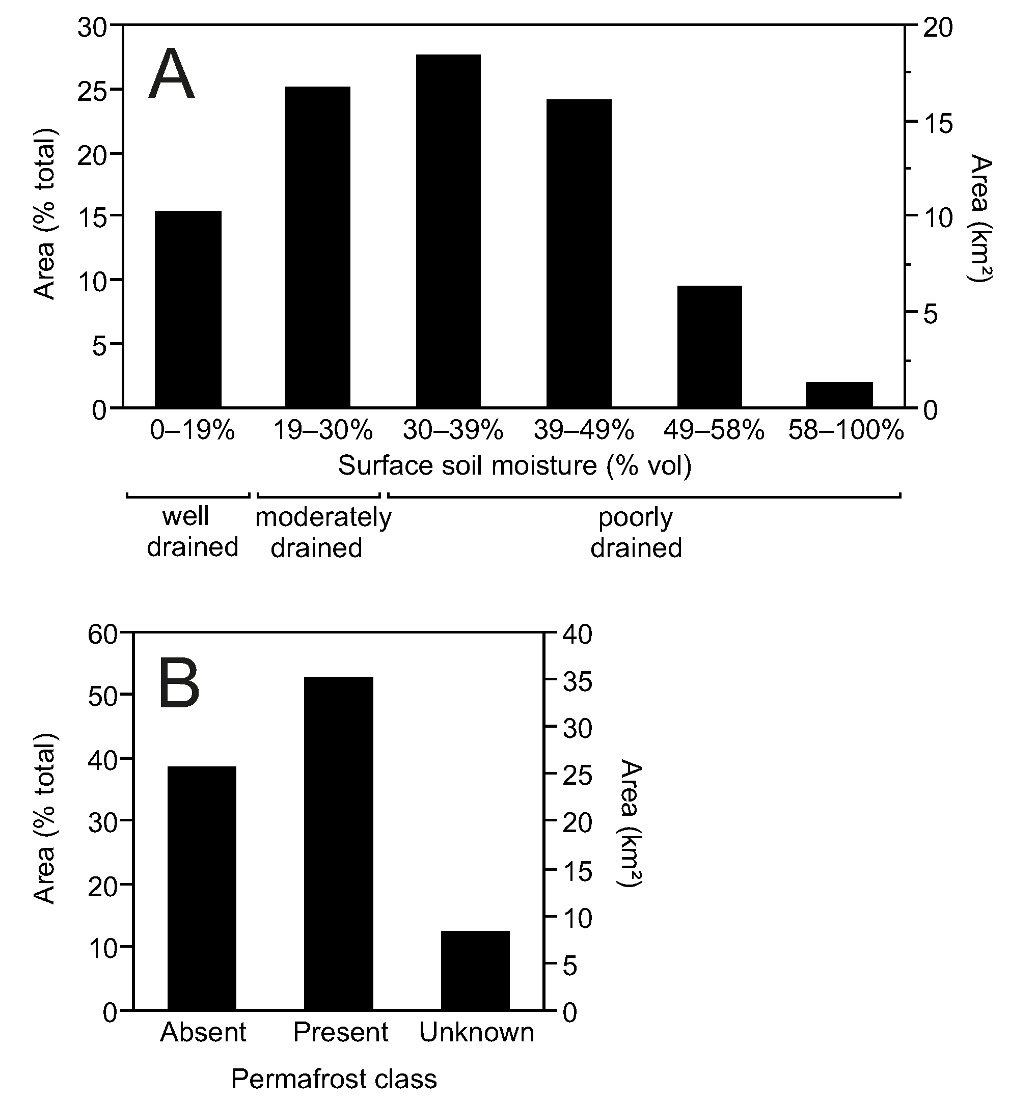
3.4. Mapping
4. Discussion
4.1. Remote Sensing Indicators of Soil Properties
4.2. Controls over Permafrost Distribution and Drainage Class
5. Conclusions
Acknowledgments
Author Contributions
Conflicts of Interest
References
- Osterkamp, T.E.; Romanovsky, V.E. Evidence for warming and thawing of discontinuous permafrost in Alaska. Permafr. Periglac. Proc. 1999, 10, 17–37. [Google Scholar] [CrossRef]
- Jafarov, E.E.; Marchenko, S.S.; Romanovsky, V.E. Numerical modeling of permafrost dynamics in Alaska using a high spatial resolution dataset. Cryosphere 2012, 6, 613–624. [Google Scholar] [CrossRef]
- Zhang, Y.; Chen, W.; Riseborough, D.W. Transient projections of permafrost distribution in Canada uring the 21st century under scenarios of climate change. Glob. Planet. Chang. 2008, 60, 443–456. [Google Scholar] [CrossRef]
- Jorgenson, M.T.; Romanovsky, V.; Harden, J.; Shur, Y.; O’Donnell, J.; Schuur, E.A.G.; Kanevskiy, M.; Marchenko, S. Resilience and vulnerability of permafrost to climate change. Can. J. For. Res. 2010, 40, 1219–1236. [Google Scholar] [CrossRef]
- Johnson, K.D.; Harden, J.W.; David McGuire, A.; Clark, M.; Yuan, F.; Finley, A.O. Permafrost and organic layer interactions over a climate gradient in a discontinuous permafrost zone. Environ. Res. Lett. 2013, 8, 035028. [Google Scholar] [CrossRef]
- Yoshikawa, K.; Bolton, W.R.; Romanovsky, V.E.; Fukuda, M.; Hinzman, L.D. Impacts of wildfire on the permafrost in the boreal forests of interior Alaska. J. Geophys. Res. 2003. [Google Scholar] [CrossRef]
- Jafarov, E.E.; Romanovsky, V.E.; Genet, H.; McGuire, A.D.; Marchenko, S.S. The effects of fire on the thermal stability of permafrost in lowland and upland black spruce forests of interior Alaska in a changing climate. Environ. Res. Lett. 2013, 8, 035030. [Google Scholar] [CrossRef]
- Brown, D.R.N.; Jorgenson, M.T.; Douglas, T.A.; Romanovsky, V.E.; Kielland, K.; Hiemstra, C.; Euskirchen, E.S.; Ruess, R.W. Interactive effects of wildfire and climate on permafrost degradation in Alaskan lowland forests. J. Geophys. Res. Biogeosci. 2015, 120, 1619–1637. [Google Scholar] [CrossRef]
- Kasischke, E.S.; Verbyla, D.L.; Rupp, T.S.; McGuire, A.D.; Murphy, K.A.; Jandt, R.; Barnes, J.L.; Hoy, E.E.; Duffy, P.A.; Calef, M.; et al. Alaska’s changing fire regime—Implications for the vulnerability of its boreal forests. Can. J. For. Res. 2010, 40, 1313–1324. [Google Scholar] [CrossRef]
- Calef, M.P.; Varvak, A.; McGuire, A.D.; Chapin, F.S.; Reinhold, K.B. Recent changes in annual area burned in interior Alaska: The impact of fire management. Earth Interact. 2015, 19, 1–17. [Google Scholar] [CrossRef]
- Genet, H.; McGuire, A.D.; Barrett, K.; Breen, A.; Euskirchen, E.S.; Johnstone, J.F.; Kasischke, E.S.; Melvin, A.M.; Bennett, A.; Mack, M.C.; et al. Modeling the effects of fire severity and climate warming on active layer thickness and soil carbon storage of black spruce forests across the landscape in interior Alaska. Environ. Rese. Lett. 2013, 8, 045016. [Google Scholar] [CrossRef]
- Schuur, E.A.; McGuire, A.D.; Schadel, C.; Grosse, G.; Harden, J.W.; Hayes, D.J.; Hugelius, G.; Koven, C.D.; Kuhry, P.; Lawrence, D.M.; et al. Climate change and the permafrost carbon feedback. Nature 2015, 520, 171–179. [Google Scholar] [CrossRef] [PubMed]
- Chapin, F.S., III; McGuire, A.D.; Ruess, R.W.; Hollingsworth, T.N.; Mack, M.C.; Johnstone, J.F.; Kasischke, E.S.; Euskirchen, E.S.; Jones, J.B.; Jorgenson, M.T.; et al. Resilience of Alaska’s boreal forest to climatic change. Can. J. For. Res. 2010, 40, 1360–1370. [Google Scholar] [CrossRef]
- Woo, M.-K.; Kane, D.L.; Carey, S.K.; Yang, D. Progress in permafrost hydrology in the new millennium. Permafr. Periglac. Processes 2008, 19, 237–254. [Google Scholar] [CrossRef]
- Jorgenson, M.T.; Osterkamp, T.E. Response of boreal ecosystems to varying modes of permafrost degradation. Can. J. For. Res. 2005, 35, 2100–2111. [Google Scholar] [CrossRef]
- Jorgenson, M.T.; Racine, C.H.; Walters, J.C.; Osterkamp, T.E. Permafrost degradation and ecological changes associated with a warming climate in central Alaska. Clim. Chang. 2001, 48, 551–579. [Google Scholar] [CrossRef]
- Koch, J.C.; Ewing, S.A.; Striegl, R.; McKnight, D.M. Rapid runoff via shallow throughflow and deeper preferential flow in a boreal catchment underlain by frozen silt (Alaska, USA). Hydrogeol. J. 2013, 21, 93–106. [Google Scholar] [CrossRef]
- Nossov, D.R.; Jorgenson, M.T.; Kielland, K.; Kanevskiy, M.Z. Edaphic and microclimatic controls over permafrost response to fire in interior Alaska. Environ. Res. Lett. 2013, 8, 035013. [Google Scholar] [CrossRef]
- Koch, J.C.; Kikuchi, C.P.; Wickland, K.P.; Schuster, P. Runoff sources and flow paths in a partially burned, upland boreal catchment underlain by permafrost. Water Resourc. Res. 2014, 50, 8141–8158. [Google Scholar] [CrossRef]
- Jorgenson, M.T.; Harden, J.; Kanevskiy, M.; O’Donnell, J.; Wickland, K.; Ewing, S.; Manies, K.; Zhuang, Q.; Shur, Y.; Striegl, R.; et al. Reorganization of vegetation, hydrology and soil carbon after permafrost degradation across heterogeneous boreal landscapes. Environ. Res. Lett. 2013, 8, 035017. [Google Scholar] [CrossRef]
- Grosse, G.; Harden, J.; Turetsky, M.; McGuire, A.D.; Camill, P.; Tarnocai, C.; Frolking, S.; Schuur, E.A.G.; Jorgenson, T.; Marchenko, S.; et al. Vulnerability of high-latitude soil organic carbon in North America to disturbance. J. Geophys. Res. 2011, 116, G00K06. [Google Scholar] [CrossRef]
- Minsley, B.J.; Abraham, J.D.; Smith, B.D.; Cannia, J.C.; Voss, C.I.; Jorgenson, M.T.; Walvoord, M.A.; Wylie, B.K.; Anderson, L.; Ball, L.B.; et al. Airborne electromagnetic imaging of discontinuous permafrost. Geophys. Res. Lett. 2012, 39. [Google Scholar] [CrossRef]
- Hachem, S.; Allard, M.; Duguay, C. Using the modis land surface temperature product for mapping permafrost: An application to northern Quebec and Labrador, Canada. Permafr. Periglac. Proc. 2009, 20, 407–416. [Google Scholar] [CrossRef]
- Langer, M.; Westermann, S.; Heikenfeld, M.; Dorn, W.; Boike, J. Satellite-based modeling of permafrost temperatures in a tundra lowland landscape. Remote Sens. Environ. 2013, 135, 12–24. [Google Scholar] [CrossRef] [Green Version]
- Westermann, S.; Østby, T.I.; Gisnås, K.; Schuler, T.V.; Etzelmüller, B. A ground temperature map of the North Atlantic permafrost region based on remote sensing and reanalysis data. Cryosphere 2015, 9, 1303–1319. [Google Scholar] [CrossRef]
- Nelson, F.E.; Shiklomanov, N.; Mueller, G.R.; Hinkel, K.M.; Walker, D.A.; Bockheim, J.G. Estimating active-layer thickness over a large region: Kuparuk River Basin, Alaska, U.S.A. Arctic Alpine Res. 1997, 29, 367–378. [Google Scholar] [CrossRef]
- Panda, S.K.; Prakash, A.; Solie, D.N.; Romanovsky, V.E.; Jorgenson, M.T. Remote sensing and field-based mapping of permafrost distribution along the Alaska Highway corridor, interior Alaska. Permafr. Periglac. Proc. 2010, 21, 271–281. [Google Scholar] [CrossRef]
- Pastick, N.J.; Jorgenson, M.T.; Wylie, B.K.; Nield, S.J.; Johnson, K.D.; Finley, A.O. Distribution of near-surface permafrost in Alaska: Estimates of present and future conditions. Remote Sens. Environ. 2015, 168, 301–315. [Google Scholar] [CrossRef]
- Karlstrom, T.N.V. Surficial Geology of Alaska; IMAP, U.S. Geological Survey: Richmond, VA, USA, 1994.
- Jorgenson, M.T.; Yoshikawa, K.; Kanevskiy, M.; Shur, Y.; Romanovsky, V.; Marchenko, S.; Grosse, G.; Brown, J.; Jones, B. Permafrost Characteristics of Alaska; Institute of Northern Engineering, University of Alaska Fairbanks: Fairbanks, AK, USA, 2008. [Google Scholar]
- Swanson, D.K. Susceptibility of permafrost soils to deep thaw after forest fires in interior Alaska, U.S.A., and some ecologic implications. Arctic Alp. Res. 1996, 28, 217–227. [Google Scholar] [CrossRef]
- Jones, J.B.; Rinehart, A.J. The long-term response of stream flow to climatic warming in headwater streams of interior Alaska. Can. J. For. Res. 2010, 40, 1210–1218. [Google Scholar] [CrossRef]
- Alaska Climate Research Center. Climate Normals from the 30-year Time Period from 1981–2010, Provided by the National Climatic Data Center. Available online: http://climate.Gi.Alaska.Edu/climate/normals (accessed on 12 May 2014).
- Bernhardt, E.L.; Hollingsworth, T.N.; Chapin, F.S., III. Fire severity mediates climate-driven shifts in understorey community composition of black spruce stands of interior Alaska. J. Veg. Sci. 2011, 22, 32–44. [Google Scholar] [CrossRef]
- Hollingsworth, T.N.; Johnstone, J.F.; Bernhardt, E.L.; Chapin, F.S. Fire severity filters regeneration traits to shape community assembly in Alaska’s boreal forest. PLoS ONE 2013, 8, e56033. [Google Scholar]
- Minsley, B.J.; Pastick, N.J.; Wylie, B.K.; Brown, D.R.N.; Kass, M.A. Evidence for nonuniform permafrost degradation after fire in boreal landscapes. J. Geophys. Res. Earth Sur. 2016, 121, 320–335. [Google Scholar] [CrossRef]
- Viereck, L.A.D.C.T.; Batten, A.R.; Wenzlick, K.J. The Alaska Vegetation Classification. General Technical Report Pnw-gtr-286; U.S. Department of Agriculture, Forest Service, Pacific Northwest Research Station: Portland, OR, USA, 1992.
- Braun-Blanquet, J. Plant Sociology: The Study of Plant Communities; Hafner: London, UK, 1965. [Google Scholar]
- Rich, P.M.; Dubayah, R.; Hetrick, W.A.; Saving, S.C. Using viewshed models to calculate intercepted solar radiation: Applications in ecology. Am. Soc. Photogramm. Remote Sens. 1994, 1994, 524–529. [Google Scholar]
- Moore, I.D.; Grayson, R.B.; Ladson, A.R. Digital terrain modelling: A review of hydrological, geomorphological, and biological applications. Hydrol. Proc. 1991, 5, 3–30. [Google Scholar] [CrossRef]
- Bourgeau-Chavez, L.L.; Kasischke, E.S.; Riordan, K.; Brunzell, S.; Nolan, M.; Hyer, E.; Slawski, J.; Medvecz, M.; Walters, T.; Ames, S. Remote monitoring of spatial and temporal surface soil moisture in fire disturbed boreal forest ecosystems with ERS SAR imagery. Int. J. Remote Sens. 2007, 28, 2133–2162. [Google Scholar] [CrossRef]
- Kasischke, E.S.; Bourgeau-Chavez, L.L.; Johnstone, J.F. Assessing spatial and temporal variations in surface soil moisture in fire-disturbed black spruce forests in interior Alaska using spaceborne synthetic aperture radar imagery—Implications for post-fire tree recruitment. Remote Sens. Environ. 2007, 108, 42–58. [Google Scholar] [CrossRef]
- U.S. Geological Survey, Department of the Interior. Product Guide: Provisional Landsat 8 Surface Reflectance Code (LaSRC) Product; Version 3; U.S. Geological Survey: Sioux Falls, SD, USA, 2016.
- Vermote, E.; Justice, C.; Claverie, M.; Franch, B. Preliminary analysis of the performance of the Landsat 8/OLI land surface reflectance product. Remote Sens. Environ. 2016. [Google Scholar] [CrossRef]
- McCune, B.; Grace, J.B. Analysis of Ecological Communities; MjM Software Design: Gleneden Beach, OR, USA, 2002. [Google Scholar]
- Jenks, G.F. The data model concept in statistical mapping. Int. Yearbook Cartogr. 1967, 7, 186–190. [Google Scholar]
- Kerr, Y.H. Soil moisture from space: Where are we? Hydrogeol. J. 2006, 15, 117–120. [Google Scholar] [CrossRef]
- National Research Council. Opportunities to Use Remote Sensing in Understanding Permafrost and Related Ecological Characteristics: Report of a Workshop; National Academies Press: Washington, DC, USA, 2014. [Google Scholar]
- French, N.H.F.; Kasischke, E.S.; Hall, R.J.; Murphy, K.A.; Verbyla, D.L.; Hoy, E.E.; Allen, J.L. Using Landsat data to assess fire and burn severity in the North American boreal forest region: An overview and summary of results. Int. J. Wildland Fire 2008, 17, 443–462. [Google Scholar] [CrossRef]
- Kimes, D.S.; Markham, B.L.; Tucker, C.J.; McMurtrey, J.E., III. Temporal relationships between spectral response and agronomic variables of a corn canopy. Remote Sens. Environ. 1981, 11, 401–411. [Google Scholar] [CrossRef]
- Ji, L.; Zhang, L.; Wylie, B.K.; Rover, J. On the terminology of the spectral vegetation index (NIR − SWIR)/(NIR + SWIR). Int. J. Remote Sens. 2011, 32, 6901–6909. [Google Scholar] [CrossRef]
- Wang, L.; Qu, J.J. NMDI: A normalized multi-band drought index for monitoring soil and vegetation moisture with satellite remote sensing. Geophys. Res. Lett. 2007, 34. [Google Scholar] [CrossRef]
- Weidong, L.; Baret, F.; Xingfa, G.; Qingxi, T.; Lanfen, Z.; Bing, Z. Relating soil surface moisture to reflectance. Remote Sens. Environ. 2002, 81, 238–246. [Google Scholar] [CrossRef]
- Romanovsky, V.E. Bonanza Creek 2—Burned: Soils, Geophysical Institute Permafrost Laboratory, University of Alaska Fairbanks. Available online: http://lapland.Gi.Alaska.Edu/vdv/index.Html (accessed on 28 July 2016).
- Alaska Climate Research Center. Acis Daily Data Browser. 2016; Volume 2016. Available online: http://climate.Gi.Alaska.Edu/acis_data (accessed on 25 March 2016).
- Viereck, L.A. Effects of fire and firelines on active layer thickness and soil temperatures in Interior Alaska. Perma. Soils 1982, 1982, 123–134. [Google Scholar]
- Van Cleve, K.; Chapin, F.S., III; Flanagan, P.W.; Viereck, L.A.; Dyrness, C.T. Forest Ecosystems in the Alaskan Taiga: A synthesis of Structure and Function; Springer-Verlag: New York, NY, USA, 1986. [Google Scholar]
- Péwé, T.L. Quaternary Geology of Alaska; United States Geological Survey: Washington, DC, USA, 1975.
- Hinzman, L.D.; Viereck, L.A.; Adams, P.C.; Romanovsky, V.E.; Yoshikawa, K. Climate and permafrost dynamics of the Alaskan boreal forest. In Alaska's Changing Boreal Forest; Chapin, F.S., III, Oswood, M.W., Van Cleve, K., Viereck, L.A., Verbyla, D.L., Eds.; Oxford University Press: New York, NY, USA, 2006. [Google Scholar]
- Rieger, S.; DeMent, J.A.; Sanders, D. Soil Survey of Fairbanks Area, Alaska. USDA Soil Conservation Service; U.S. Government Printing Office: Washington, DC, USA, 1963.
- Ping, C.L.; Michaelson, G.J.; Packee, E.C.; Stiles, C.A.; Swanson, D.K.; Yoshikawa, K. Soil catena sequences and fire ecology in the boreal forest of Alaska. Soil Sci. Soc. Am. J. 2005, 69, 1761. [Google Scholar] [CrossRef]
- Barrett, K.; Kasischke, E.S.; McGuire, A.D.; Turetsky, M.R.; Kane, E.S. Modeling fire severity in black spruce stands in the Alaskan boreal forest using spectral and non- spectral geospatial data. Remote Sens. Environ. 2010, 114, 1494–1503. [Google Scholar] [CrossRef]
- Kane, E.S.; Kasischke, E.S.; Valentine, D.W.; Turetsky, M.R.; McGuire, A.D. Topographic influences on wildfire consumption of soil organic carbon in interior Alaska: Implications for black carbon accumulation. J. Geophys. Res. 2007, 112. [Google Scholar] [CrossRef]
- Hinzman, L.D.; Bolton, W.R.; Petrone, K.C.; Jones, J.B.; Adams, P.C. Watershed hydrology and chemistry in the Alaskan boreal forest: The central role of permafrost. In Alaska's Changing Boreal Forest; Chapin, F.S., III, Oswood, M.W., Van Cleve, K., Viereck, L.A., Verbyla, D., Eds.; Oxford University Press: New York, NY, USA, 2006; pp. 269–284. [Google Scholar]
- Bolton, W.R.; Hinzman, L.; Yoshikawa, K. Stream Flow Studies in a Watershed Underlain by Discontinuous Permafrost; American Water Resources Association: Anchorage, AK, USA, 2000. [Google Scholar]
- Shenoy, A.; Johnstone, J.F.; Kasischke, E.S.; Kielland, K. Persistent effects of fire severity on early successional forests in interior Alaska. For. Ecol. Manag. 2011, 261, 381–390. [Google Scholar] [CrossRef]


| Site | Elevation (m) | Slope (°) | Organic Layer Thickness (cm) | Soil Temperature at 1 m (°C) | Soil Moisture (% vol.) | Vegetation Type |
|---|---|---|---|---|---|---|
| NC01 | 599 | 13 | 24 | 0.24 | 33 | Low shrub |
| NC02 | 613 | 12 | 22 | 5.44 | 7 | Low shrub |
| NC03 | 626 | 15 | 8 | 5.25 | 7 | Low shrub |
| NC04 | 632 | 8 | 11 | −0.04 | 30 | Low shrub |
| NC05 | 617 | 20 | 8 | 4.77 | 23 | Low shrub |
| NC06 | 633 | 13 | 13 | 3.43 | 16 | Low shrub |
| NC07 | 633 | 12 | 9 | 1.01 | 34 | Low shrub |
| NC09 | 565 | 9 | 13 | 0.74 | 53 | Low shrub |
| NC11 | 588 | 10 | 14 | −0.29 | 40 | Low shrub |
| NC12 | 608 | 12 | 18 | 0.18 | 40 | Low shrub |
| NC13 | 653 | 13 | 9 | 3.65 | 25 | Low shrub |
| NC14 | 698 | 12 | 6 | 5.81 | 9 | Bryoid herbaceous |
| NC15 | 700 | 11 | 15 | 3.57 | 7 | Low shrub |
| NC16 | 690 | 13 | 12 | 6.65 | 28 | Bryoid herbaceous |
| NC17 | 658 | 15 | 10 | 4.66 | 24 | Low shrub |
| NC18 | 778 | 29 | 4 | 4.20 | 22 | Grassy herbaceous |
| NC19 | 738 | 16 | 17 | 0.85 | 21 | Low shrub |
| NC20 | 701 | 26 | 10 | 5.11 | 18 | Low shrub |
| NC21 | 724 | 16 | 24 | 0.33 | 51 | Low shrub |
| NC22 | 776 | 16 | 7 | 4.20 | 22 | Bryoid herbaceous |
| NC24 | 680 | 14 | 11 | 5.68 | 30 | Bryoid herbaceous |
| NC25 | 506 | 2 | 7 | 4.09 | 26 | Low shrub |
| NC26 | 544 | 9 | 12 | 0.28 | 52 | Low shrub |
| NC27 | 579 | 11 | 14 | −0.22 | 65 | Shrub-tussock |
| NC28 | 584 | 8 | 26 | −0.24 | 42 | Shrub-tussock |
| NC29 | 609 | 13 | 13 | 2.53 | 31 | Low shrub |
| NC30 | 601 | 16 | 8 | 0.12 | 36 | Low shrub |
| WTCR-B1 | 590 | 9 | 25 | −0.17 | 48 | Shrub-tussock |
| WTCR-B2 | 606 | 13 | 12 | 4.14 | 11 | Low shrub |
| WTCR-B3 | 619 | 14 | 15 | 4.40 | 16 | Low shrub |
| Satellite/Sensor | Date | Frame | Path |
|---|---|---|---|
| ALOS-PALSAR | 8 August 2009 | 1300 | 253 |
| ALOS-PALSAR | 23 September 2009 | 1300 | 253 |
| ALOS-PALSAR | 11 August 2010 | 1300 | 253 |
| ALOS-PALSAR | 26 September 2010 | 1300 | 253 |
| Date | Path | Row | |
| Landsat 8 OLI | 2 June 2013 | 69 | 14 |
| Landsat 8 OLI | 18 June 2013 | 69 | 14 |
| Landsat 8 OLI | 13 July 2013 | 68 | 14 |
| Landsat 8 OLI | 12 August 2013 | 70 | 14 |
| Landsat 8 OLI | 15 September 2013 | 68 | 14 |
| Landsat 8 OLI | 20 May 2014 | 69 | 14 |
| Landsat 8 OLI | 30 July 2014 | 70 | 14 |
| Landsat 8 OLI | 24 August 2014 | 69 | 14 |
| Landsat 8 OLI | 9 September 2014 | 69 | 14 |
| Landsat 8 OLI | 18 September 2014 | 68 | 14 |
| Landsat 8 OLI | 23 May 2015 | 69 | 14 |
| Landsat 8 OLI | 15 June 2015 | 70 | 14 |
| Landsat 8 OLI | 4 August 2015 | 68 | 14 |
| Landsat 8 OLI | 3 September 2015 | 70 | 14 |
| Landsat 7 ETM+ | 27 May 2002 | 69 | 14 |
| Landsat 7 ETM+ | 22 July 2005 | 69 | 14 |
| Variable | Source |
|---|---|
| Topographic | |
| Aspect | LiDAR DEM |
| CTI | LiDAR DEM |
| Curvature | LiDAR DEM |
| Elevation | LiDAR DEM |
| Slope | LiDAR DEM |
| Solar radiation | LiDAR DEM |
| Radar | |
| HH-PC1 | ALOS-PALSAR |
| HH-PC2 | ALOS-PALSAR |
| HH-PC3 | ALOS-PALSAR |
| HH-PC4 | ALOS-PALSAR |
| HV-PC1 | ALOS-PALSAR |
| HV-PC2 | ALOS-PALSAR |
| HV-PC3 | ALOS-PALSAR |
| HV-PC4 | ALOS-PALSAR |
| Optical | |
| dNBR | Landsat 7 ETM+ |
| NDII6 | Landsat 8 OLI |
| NDII7 | Landsat 8 OLI |
| NDVI | Landsat 8 OLI |
| Axis 1 | Axis 2 | ||||||
|---|---|---|---|---|---|---|---|
| r | R2 | tau | r | R2 | tau | ||
| Vegetation type (% cover) | |||||||
| Dwarf shrubs | −0.55 | 0.31 | −0.37 | 0.12 | 0.01 | 0.05 | |
| Low shrubs | −0.63 | 0.39 | −0.40 | −0.14 | 0.02 | −0.04 | |
| Grasses | 0.66 | 0.43 | 0.51 | 0.05 | 0.00 | −0.07 | |
| Plant species (% cover) | |||||||
| Tall shrubs | Alnus incana ssp. crispa | 0.22 | 0.05 | 0.08 | −0.52 | 0.27 | −0.37 |
| Low shrubs | Rhododendron spp. | −0.69 | 0.47 | −0.46 | −0.38 | 0.15 | −0.28 |
| Rosa acicularis | 0.40 | 0.16 | 0.30 | 0.49 | 0.24 | 0.34 | |
| Vaccinium uliginosum | −0.53 | 0.28 | −0.37 | 0.49 | 0.24 | 0.43 | |
| Dwarf shrubs | Vaccinium vitis-idaea | −0.51 | 0.26 | −0.43 | 0.12 | 0.02 | 0.11 |
| Forbs | Aster sibirica | 0.55 | 0.30 | 0.34 | −0.07 | 0.01 | −0.03 |
| Cornus canadensis | 0.60 | 0.36 | 0.47 | −0.30 | 0.09 | −0.35 | |
| Chamerion angustifolium | 0.46 | 0.21 | 0.40 | 0.56 | 0.31 | 0.44 | |
| Rubus chamaemorus | −0.72 | 0.52 | −0.59 | −0.43 | 0.19 | −0.30 | |
| Sedges | Carex bigelowii | 0.53 | 0.28 | 0.48 | −0.18 | 0.03 | −0.20 |
| Sedge tussocks | Eriophorum vaginatum | −0.62 | 0.39 | −0.68 | 0.02 | 0.00 | 0.19 |
| Mosses | Ceratodon purpureus | 0.69 | 0.48 | 0.45 | −0.07 | 0.01 | 0.05 |
| Polytrichum juniperinum | 0.47 | 0.22 | 0.43 | 0.01 | 0.00 | −0.19 | |
| Sphagnum spp. | −0.58 | 0.33 | −0.55 | −0.19 | 0.04 | −0.21 | |
| Soil properties | |||||||
| OLT | −0.62 | 0.38 | −0.49 | −0.15 | 0.02 | −0.01 | |
| Soil moisture, 20 cm | −0.53 | 0.28 | −0.43 | 0.22 | 0.05 | 0.22 | |
| Soil temperature, 1 m | 0.84 | 0.71 | 0.69 | 0.03 | 0.00 | −0.03 | |
| Remote sensing variables | |||||||
| Elevation | 0.44 | 0.19 | 0.35 | −0.62 | 0.38 | −0.45 | |
| NDII7 | −0.73 | 0.54 | −0.57 | 0.02 | 0.00 | 0.03 | |
| NDVI | −0.68 | 0.46 | −0.42 | −0.04 | 0.00 | −0.03 | |
| dNBR | 0.60 | 0.35 | 0.52 | 0.02 | 0.00 | 0.03 | |
| Remote Sensing Dataset | Variable | Soil Moisture | Soil Temperature | Organic Layer Thickness | |||
|---|---|---|---|---|---|---|---|
| ρ | Prob > |ρ| | ρ | Prob > |ρ| | ρ | Prob > |ρ| | ||
| Topographic | Aspect | 0.21 | 0.2638 | −0.12 | 0.5271 | −0.33 | 0.0780 |
| CTI | −0.15 | 0.4409 | 0.08 | 0.6611 | −0.01 | 0.9805 | |
| Curvature | 0.22 | 0.2476 | −0.04 | 0.8336 | −0.03 | 0.8767 | |
| Elevation | −0.53 | 0.0025 | 0.54 | 0.0023 | −0.28 | 0.1275 | |
| Slope | −0.38 | 0.0395 | 0.48 | 0.0078 | −0.31 | 0.0961 | |
| Solar radiation | −0.07 | 0.7042 | 0.20 | 0.2975 | 0.13 | 0.5020 | |
| Radar | HH-PC1 | −0.21 | 0.2764 | −0.03 | 0.8923 | −0.03 | 0.8840 |
| HH-PC2 | 0.08 | 0.6697 | 0.02 | 0.9015 | −0.03 | 0.8656 | |
| HH-PC3 | 0.29 | 0.1251 | −0.29 | 0.1234 | 0.02 | 0.9025 | |
| HH-PC4 | 0.07 | 0.7042 | −0.10 | 0.6084 | −0.02 | 0.9006 | |
| HV-PC1 | 0.42 | 0.0200 | −0.36 | 0.0516 | 0.35 | 0.0580 | |
| HV-PC2 | 0.12 | 0.5419 | −0.03 | 0.8573 | 0.14 | 0.4651 | |
| HV-PC3 | 0.22 | 0.2486 | −0.03 | 0.8812 | −0.17 | 0.3597 | |
| HV-PC4 | −0.07 | 0.7164 | −0.08 | 0.6894 | −0.08 | 0.6680 | |
| Optical | dNBR | −0.53 | 0.0026 | 0.64 | 0.0001 | −0.29 | 0.1201 |
| NDII6 | 0.66 | <0.0001 | −0.81 | <0.0001 | 0.32 | 0.0874 | |
| NDII7 | 0.69 | <0.0001 | −0.83 | <0.0001 | 0.37 | 0.0456 | |
| NDVI | 0.39 | 0.0345 | −0.57 | 0.0009 | 0.35 | 0.0573 | |
© 2016 by the authors; licensee MDPI, Basel, Switzerland. This article is an open access article distributed under the terms and conditions of the Creative Commons Attribution (CC-BY) license (http://creativecommons.org/licenses/by/4.0/).
Share and Cite
Brown, D.R.N.; Jorgenson, M.T.; Kielland, K.; Verbyla, D.L.; Prakash, A.; Koch, J.C. Landscape Effects of Wildfire on Permafrost Distribution in Interior Alaska Derived from Remote Sensing. Remote Sens. 2016, 8, 654. https://doi.org/10.3390/rs8080654
Brown DRN, Jorgenson MT, Kielland K, Verbyla DL, Prakash A, Koch JC. Landscape Effects of Wildfire on Permafrost Distribution in Interior Alaska Derived from Remote Sensing. Remote Sensing. 2016; 8(8):654. https://doi.org/10.3390/rs8080654
Chicago/Turabian StyleBrown, Dana R.N., Mark T. Jorgenson, Knut Kielland, David L. Verbyla, Anupma Prakash, and Joshua C. Koch. 2016. "Landscape Effects of Wildfire on Permafrost Distribution in Interior Alaska Derived from Remote Sensing" Remote Sensing 8, no. 8: 654. https://doi.org/10.3390/rs8080654