A Sparsity-Based Regularization Approach for Deconvolution of Full-Waveform Airborne Lidar Data

Abstract

Full-waveform lidar systems capture the complete backscattered signal from the interaction of the laser beam with targets located within the laser footprint. The resulting data have advantages over discrete return lidar, including higher accuracy of the range measurements and the possibility of retrieving additional returns from weak and overlapping pulses. In addition, radiometric characteristics of targets, e.g., target cross-section, can also be retrieved from the waveforms. However, waveform restoration and removal of the effect of the emitted system pulse from the returned waveform are critical for precise range measurement, 3D reconstruction and target cross-section extraction. In this paper, a sparsity-constrained regularization approach for deconvolution of the returned lidar waveform and restoration of the target cross-section is presented. Primal-dual interior point methods are exploited to solve the resulting nonlinear convex optimization problem. The optimal regularization parameter is determined based on the L-curve method, which provides high consistency in varied conditions. Quantitative evaluation and visual assessment of results show the superior performance of the proposed regularization approach in both removal of the effect of the system waveform and reconstruction of the target cross-section as compared to other prominent deconvolution approaches. This demonstrates the potential of the proposed approach for improving the accuracy of both range measurements and geophysical attribute retrieval. The feasibility and consistency of the presented approach in the processing of a variety of lidar data acquired under different system configurations is also highlighted.

1. Introduction

Laser remote sensing is being increasingly adopted as a useful tool for capturing 3D information in conjunction with other descriptive data (e.g., intensities) from targets, and it is now being utilized for a number of applications. These include classification [1,2], object extraction and 3D reconstruction [3], vegetation structure characterization [4,5] and digital elevation model (DEM) generation [6].

Discrete lidar systems estimate the distance between the sensor and the target through precise measurement of the transit time between the emitted and backscattered laser pulse using real-time echo detection. Such discrete systems generally do not specify the exploited pulse detection method [4,7,8] and only provide range information with a single backscatter intensity value, inherently neglecting the backscattering characteristics of the illuminated target. In contrast, highly accurate pulse detection and subsequent range measurement is potentially possible in full-waveform lidar, subject to the methods adopted for data post-processing. Full-waveform lidar systems record the entire backscattered signal, providing a range measurement, a measure of the energy reflected from the target and the distribution of the returned energy along the laser path. Physical characteristics of the underlying target can then be revealed, thus enhancing the capability of the lidar system to yield both geometric and physical information of targets for a broad range of applications.

Classical pulse detectors, in ideal conditions, can only provide the range and amplitude values of pulses, without allowing removal of the effect of the transmitted pulse or the delivery of echo parameters and radiometric information about targets [9,10]. Moreover, even though accurate range determination is an important aspect in processing full-waveform lidar data, restoring the target response is a key prerequisite step not only for range measurement but also for the extraction of geophysical attributes of the target. The target cross-section is an attribute that is independent of the instrument [11,12] and is more related to the effective target area (and its shape) inside the footprint, as well as to its reflectivity and the direction of the incoming light [13,14]. The scattering cross-section, which provides insight into geophysical characteristics and target roughness [11,15] is an issue of considerable significance in laser radar remote sensing [14,16] and it can be recovered in the case of full-waveform lidar [8].

In addition, more useful attributes can be extracted by analyzing the lidar signal geometry. Recovery of overlapping signals and weak echoes is also feasible and advantageous in full-waveform lidar to avoid both misinterpretation and incorrect estimation of the range. The additional pulses, which may not be detected by discrete return systems, along with their associated features, can provide useful inputs for further processing, e.g., for segmentation, classification and 3D modelling [1,17,18,19].

A lidar waveform is generally complex, particularly in vegetated areas. Overlapping waveforms are recorded as a consequence of a finite detection time, noise, impulse function of the receiver and changes in the transmitted pulse, leading to resolution degradation for closely located targets along the laser beam [20]. Critical to the success of full-waveform lidar systems is the ability to understand and interpret the shape of the recorded return laser pulse so as to separate fine object structures. A number of lidar waveform processing approaches have been developed [14,21,22,23] and these have generally concentrated on decomposition of the waveform into a series of parametric (e.g., Gaussian) pulses so as to extract the range, amplitude and pulse width. Since the lidar waveform is essentially the result of a convolution of the system transmitted laser pulse and the target cross-section, the retrieval of target properties requires a deconvolution of the returned waveform. In addition, account must be taken of the fact that incorporation of the system properties delivers a more meticulous analysis of the waveform [24]. In particular, deconvolution essentially removes the effect of the system signal, resulting in an unbiased estimate of the target cross-section.

This paper proposes a new signal deconvolution approach for efficient temporal target cross-section retrieval from full-waveform lidar. This is achieved through a regularization approach with sparsity constraints that can be efficiently solved when cast in the form of a convex optimization problem. An efficient way to determine the optimal regularization parameter value, a critical issue in regularization, through utilization of the L-curve method and a search for the bending point on such a curve, is introduced. In order to model and estimate the system waveform, in situations where it is unavailable, an appropriate approach is proposed through the use of blind deconvolution of waveforms recorded over nearly flat targets, without requiring information about the surface reflectivity.

The remainder of the paper is organized as follows: Section 2 provides a review of research on lidar waveform processing. Following this, in Section 3, the proposed lidar waveform deconvolution method is presented through reference to the fundamentals of laser propagation, regularization for deconvolution and estimation of an optimal regularization parameter value. In Section 4, the experimental tests with both synthetic and real data covering different test sites are presented, and performance of the proposed lidar waveform deconvolution approach is evaluated. Concluding remarks are offered in Section 5.

2. Review of Related Research

With full-waveform lidar systems increasingly being adopted, improved methods are being developed for the processing of lidar waveforms. Approaches adopted in the literature can be categorized as either decomposition- or deconvolution-based, where the former approaches fit parametric functions to the received signals before retrieval of the target cross-section.

2.1. Decomposition Methods

Gaussian waveform decomposition methods for the extraction of a parametric description of the pulse properties, including range, width and amplitude, have been developed for instance by Hofton et al. [21] for a laser vegetation imaging sensor (LVIS), by Persson et al. [22] for the TopEye Mark II lidar system and by Wagner et al. [14] for small footprint data. Generally, a set of Gaussian functions is considered to both fit to the received backscattered waveform and to characterize each pulse shape in this approach. Gaussian decomposition and other similar decomposition methods have been extensively used to interpret targets related to the backscattered waveform in urban and forested areas [1,2,17,25]. However, this method is considered challenging in the case of echoes with low signal strength (low SNR) and it is deficient in its calculation of the cross-section in complex waveforms. The method also requires initial determination of the number of targets [16,18,23,26], which is sometimes impractical or of high computational cost. In addition, a symmetric function might not always be sufficiently accurate to describe the target characteristics [17,27]. Furthermore, Gaussian decomposition has a vulnerability in that it can result in a null solution or even negative amplitudes in some cases [11,18]. The possibility of failure in the detection of peaks and in the fitting of Gaussian functions to complex waveforms, principally due to a high dependency on local maxima, has been reported [18]. These problems cause the range accuracy to deteriorate, which then impacts upon subsequent lidar processing.

More complicated parametric distribution functions for the extraction of pulse parameters have been investigated. Chauve et al. [27] extracted target attributes from pulses by utilizing a mixture of the generalized Gaussian and Lognormal functions, with an improved global fitting for the former, and a better pulse fitting result locally in asymmetric cases for the latter. This work was extended by Chauve et al. [17] to suppression of the ringing effect, and the results were utilized in DTM and Canopy Height Model (CHM) extraction, as well as for accurate determination of tree height. A low rate of height underestimation in the CHM generation was reported by the authors. A set of parametric pulse shapes (the Burr, Nakagami and generalized Gaussian models) have been considered by Mallet et al. [23], where it was pointed out that the efficacy of the approach when applied to object classification was inadequate. However, more accurate results could be achieved when these waveform features were utilized in combination with geometric attributes. Lin et al. [18] studied weak and overlapping pulses and reported higher obtainable accuracies in multi-target separation using a rigorous pulse fitting method, however at very high computational cost.

In general, decomposition methods all attempt to fit a function (or functions) to the received waveform and extract related attributes from the parametric function(s). However, parameter estimation based only on the received waveform and not on the perceived deviations in the transmitted pulse may not in general be valid [11]. In addition, direct extraction of the range from the maximal amplitude value is not recommended since the signal pulse may be altered as a result of superimposing different target responses [12,15]. It has therefore been suggested that recording both the received and the outgoing waveforms is indispensable [12]. Disentanglement of the received waveform from the instrument and estimation of a signal more related to the target response can be achieved by exploiting deconvolution approaches. Reconstruction of instrument-independent target features by deconvolution can result in precise characterization of the actual response of the targets [5,12].

2.2. Deconvolution Methods

The retrieval of target cross-section by signal deconvolution is an ill-posed problem and a unique solution is usually not obtainable without the imposition of appropriate solution constraints [16]. Unlike Gaussian decomposition, deconvolution does not require information regarding the number of signal peaks and there is no essential assumption regarding the pulse shape [7,26].

An encouraging reported approach for both retrieval of the target response and improved range estimation is Wiener filtering [5,12,19,20]. The Wiener filter minimizes the mean square error between the approximated cross-section and the true surface response. However, negative amplitudes and ringing effects usually appear in signals restored by using this method [19,20].

In another approach, reported in Roncat et al. [11], the differential cross-section is measured by using B-splines as a linear deconvolution approach, with the assumption that pulses are not necessarily symmetric. Negative amplitude values were reported in the resulting cross-section profile.

Wu et al. [28] defined four steps to form a pre-processing sequence for calibrating full-waveform lidar data based upon synthetic waveform generation from the DIRSIG simulation model. The defined steps are noise removal, signal deconvolution, geometric correction, and angular rectification. Among these, deconvolution has emerged as the most critical for waveforms from lidar with a nadir scan angle, while geometric calibration is the principal enhancement factor for off-nadir scanning. The Richardson-Lucy (R-L) method was adopted in the deconvolution investigation. While this method is efficient in most cases, underestimation of the amplitude values and the occasional missing of pulses, in addition to essential speculation on the number of iterations by the user, remain its main shortcomings. It is noticeable that increasing the number of iterations does not generally guarantee that the optimal results will be achieved because after some iterations the quality of the restored signal can deteriorate and spurious pulses will be generated as a result of noise amplification [29,30]. As also reported in Neilsen [31], increasing the number of iterations in the R-L algorithm has an adverse effect on the range resolution and can cause an increase in the range error.

Deconvolution of the received waveform can be accomplished by regularization techniques, as demonstrated in Wang et al. [16]. This approach can restrain noise propagation and improve computational efficiency. However, the method utilized to estimate the regularization parameter, namely the discrepancy principle, demands that the noise level in the waveform be known, which is not practical in the case of real data and hence the method is restricted in its application.

Negative amplitude values can be avoided by using iterative deconvolution methods, e.g., the Gold and R-L methods. Such approaches can also minimize smearing effects (signal distortion level) on the signal and they have been shown to be effective in retrieving pulses in lidar data [20,26,28], as well as in other fields of research [32]. Wu et al. [20] reported that not all peaks can be detected. This can cause errors in range estimation and lead to false target detection. Moreover, the solutions generated by these methods can be significantly affected by the number of iterations. Thus, any invalid assumptions can lead to inaccurate results.

Application of compressed sensing in lidar processing using synthetic data has also attracted limited attention [33,34]. In this case, inclusion of lidar data compression in the acquisition was endeavored in order to cope with large data volume. The transmitted waveform of the chaotic type presented in [34] was described to compress waveform data whilst allowing retrieval of the range information using the DIRSIG simulation model. Higher SNR were perceived in case of chaotic signals than that of using linear Frequency Modulated (LFM) signals. Reconstructing of randomly generated surfaces was investigated at different complexity levels through implementing compressed sensing in [33]. The edges connecting facets could not be retrieved in [33] when the proposed method is based on the total variation algorithm, while such an algorithm is known for successful retrieval of edges. In addition, the complexity of surfaces is required in [33] to appropriately retrieve the surface.

The present paper explores the theory of signal deconvolution for improved full-waveform lidar processing through a reliable sparsity-constrained regularization. In addition, the estimation of system waveforms based on blind deconvolution is presented and an approach to the determination of regularization parameters is proposed.

3. Methodology

The proposed approach explores signal deconvolution for target cross-section retrieval. Following a brief review of two major classes of deconvolution methods and a justification for selection of the most efficient group, the sparsity-constrained regularization for deconvolution is presented and the approaches to the sparse solution are detailed. A method based on the L-curve for the determination of the regularization parameter is then proposed and a new approach using blind deconvolution for estimation of the system waveform is developed.

3.1. Deconvolution for Cross-Section Retrieval

Deconvolution is the process of signal and image restoration in a system with linear and shift-invariant characteristics [35]. There are two major classes of deconvolution methods, namely direct and iterative. Of the latter group, the Gold [36] and R-L [37,38] are recognized as approaches that provide signals/images of positive values, provided that the input raw waveform values are also non-negative [32]. Direct deconvolution methods, on the other hand, involve a regularization parameter, which controls the level of restoration. The number of optimal iterations in the iterative methods is of the same level of significance as the regularization parameter in the direct deconvolution methods, and different values for each of these parameters will surely result in a different solution, and sometimes may deliver over-smooth or noisy results. Unfortunately, selection of the optimal number of iterations is still a challenge and changes in this number may result in varying levels of signal recovery (overestimation or underestimation). In this research, direct deconvolution methods are investigated for two main reasons. First, an optimal regularization parameter can be more appropriately determined, so controlling the solution will therefore not be problematic. Second, this class of deconvolution approaches makes it possible to incorporate additional constraints and conditions [39] and, in turn, is more flexible compared to the iterative approaches.

3.1.1. Target Cross-Section Retrieval

As mentioned, the process of target cross-section retrieval is an ill-posed problem, and it requires consideration of additional conditions. In this situation, substantial perturbations can occur in the restored signal as a consequence of either trivial changes in the received waveform or noise in the waveform. Therefore, regularization is a necessary way to achieve a stable solution to the deconvolution problem by providing an approximation after imposing additional constraints [40]. In order to accomplish the condition, it is necessary to determine an optimal regularization parameter by an appropriate method [41].

The target cross-section for an extended non-overlapping diffuse surface with reflectivity $\mathsf{\rho }$, the solid angle of π steradians, and under incidence angle θ, will be [13]:

$${\sigma }_{ex}=4\rho d_A\cos \left(\theta \right)$$

(1)

where $d_A=\frac{\pi R^2{\beta }_t^2}{4}$ is the effective target area illuminated by the laser footprint, for a transmitter with a typical disk-like aperture with ${\beta }_t$ as its beamwidth, at the range R.

The received signal power $P_r\left(t\right)$ at the receiver is essentially a convolution of the point spread function (system waveform) $S\left(t\right)$ and the unknown differential target cross-section $\sigma \left(t\right)$, along with an additive noise term $n\left(t\right)$, and it can be expressed through the following equation [16]:

$$P_r\left(t\right)=S\left(t\right)*\sigma \left(t\right)+n\left(t\right)$$

(2)

In Equation (2), any possible loss of the transmitted pulse energy when intercepted by multi-return targets (e.g., vegetation) is ignored, and $\sigma \left(t\right)$ represents only the cross-section of the effective areas in multi-return targets. In order to recover the target response, the effect of convolution in Equation (2) should be compensated through deconvolution.

3.1.2. Sparsity-Constrained Regularization

Throughout the rest of this paper, waveforms are treated as discrete signals. The general form of the variational regularization, used to retrieve the temporal target cross-section $\sigma$ in Equation (2), is expressed by Gunturk and Li [35] as:

$$\sigma =\text{arg}\underset{\sigma }{\min }\{{\Vert P-S\sigma \Vert }^2+\lambda \phi \left(\sigma \right)\}$$

(3)

where, $\lambda \in \left(0,\infty \right)$ is the regularization parameter, $\phi (.)$ is the regularization function, $\Vert .\Vert$ denotes the Euclidean norm, P is a vector representing the received waveform and S is the blur matrix comprised of the system waveform.

This objective function seeks a solution by minimizing the sum of squared dissimilarities between the estimated and the desired solution, while imposing a constraint on the solution to achieve desirable properties. The first term (residual) in Equation (3) measures how the solution fits the data, and the regularization term introduces prior information about the solution and imposes a penalty on large amplitude values of the retrieved signal [42]. The selection of λ should be made with caution, since it controls the level of signal restoration and different values result in different solutions, and sometimes may deliver over-smooth or noisy results.

The regularization function plays a critical role and different regularization functions, appropriate to different specific applications have been introduced in the literature [35]. Tikhonov regularization [43], which is the most common variational regularization method, makes use of the regularization function $\phi \left(\sigma \right)={\Vert L\sigma \Vert }^2$, where L is a regularization operator. Through a consideration of prior information and adherence to the Gibbs distribution, the signal probability is determined by measuring the deviation from smoothness [44]. This is a convex quadratic optimization problem and can be solved with different approaches [42]. However, the Tikhonov regularization function, which utilizes the l₂-norm, exaggerates data smoothness. The shape of the penalty function affects the solution. When using the l₂-norm, as in Tikhonov regularization, large residuals are allocated a higher weight than small residuals [42], and also small elements are revealed in the obtained signal associated with small singular values [45]. As a result, Tikhonov regularization may cause oscillation around principal peaks, restoring signals with under-estimated amplitude values, and it may also generate negative amplitude values [32,46]. To avoid such problems, sparsity constraints have been introduced as an appropriate technique in regularization [35,47]. The term sparsity refers to the minimum number of nonzero elements within a desired solution that can be included in the objective function through use of the l₀-norm.

Sparse formulation of the regularization solution can be expressed as follows:

$$\sigma =\text{arg}\underset{\sigma }{\min }\{{\Vert P-S\sigma \Vert }^2+\lambda {\Vert L\sigma \Vert }_0\}$$

(4)

where ${\Vert .\Vert }_0$ represents the sparsity constraint on the solution.

Among the methods for sparse solution, greedy pursuit methods and convex optimization have proven to be effective and are broadly used whilst also being computationally tractable [48]. The effectiveness of convex relaxation techniques in achieving an appropriate solution for the sparsity-constrained regularization has been verified to a large extent, especially in cases involving high noise levels. More importantly, a local optimal point, where it exists in convex optimization, is also globally optimal [42]. In convex optimization methods the idea is to impose a relaxation and replace the l₀-norm in Equation (4) by its closest convex form, the l₁-norm, such that standard methods in convex optimization can be adopted [48]. The reason for the substitution of the l₀-norm with the l₁-norm is that the former results in impractical methods because of the high computational complexity [35]. The cost function is therefore altered to:

$$\sigma =\text{arg}\underset{\sigma }{\min }\{{\Vert P-S\sigma \Vert }^2+\lambda {\Vert L\sigma \Vert }_1\}$$

(5)

In contrast with Tikhonov regularization, substantial weight is assigned to small residuals in the case of the l₁-norm penalty functions in sparse regularization, hence resulting in even smaller residuals [42]. Additionally, the l₁-norm solution does not produce signal elements relevant to small singular values [45]. Large amplitude values can be recovered by imposing smaller penalties when adopting the l₁-norm solution, in lieu of that of the l₂-norm [44]. Also, the oscillations of Tikhonov regularization can be controlled to a large extent by this solution. The l₁-norm regularization method has been adopted in many applications, from signal/image deconvolution to feature selection, and to compressed sensing [35,49]. In the case of waveform deconvolution, small elements of the target response vector are encouraged to become zero, which is an aim of sparse solutions.

A sparse solution for Equation (5) always exists as a nonlinear function of the noisy observations, although it is not necessarily unique. However, solving this problem involves high computational complexity compared to its counterpart in the l₂-norm solution due to its non-differentiability [50].

By recasting waveform restoration into the form of the convex problem in Equation (5), advanced approaches in convex optimization can be explored. Iterative Shrinkage/Thresholding (IST) methods, based on either the proximal gradient or expectation-maximization [35,51], together with interior-point methods [42,50,51], are noteworthy examples. To exploit the latter group, the convex optimization should be converted to a quadratic form, second-order cone programming (SOCP) problem [50,51], where interior-point methods have proven to be effective in producing highly accurate results compared with other methods such as the barrier method [42].

3.1.3. Optimization with SOCP

Linear and convex quadratic problems can be expressed in the style of nonlinear convex SOCP problems, which can be efficiently solved by primal-dual methods [52,53]. The SOCP form of the main objective function in Equation (5), with $\sigma ,u$ and $v$ as the variables, is written as [42]:

$$\text{min u}+\lambda vs.t.\Vert S\sigma -P\Vert \le u,{\Vert \sigma \Vert }_1\le v$$

(6)

Because of the convexity of the cost function and the second-order cone constraint, the SOCP problem in Equation (6) is a convex problem. In primal-dual interior-point methods, Newton’s method is employed to calculate the search direction on the central path, from the modified Karush-Kuhn-Tucker (KKT) conditions. Assigning the residual components (the dual, centrality and primal residuals) to zero, the Newton step can be obtained as the primal-dual search direction by solving a set of equations [42].

3.1.4. Blur Matrix Structure

The blur matrix S in Equation (5) should be structured as a function of the system waveform elements. Undesirable oscillations will likely be revealed in cases where an inappropriate blur model is defined [54]. The blur matrix can be constructed in the following form [55], where h_i represents the ith element of the system waveform:

$$S=\left[\begin{array}{ccccc}{h}_1& 0& 0& \cdots & 0\\ h_2& h_1& 0& \cdots & 0\\ ⋮& ⋮& ⋮& \ddots & ⋮\\ h_n& h_{n-1}& h_{n-2}& \cdots & 0\\ 0& h_n& h_{n-1}& \cdots & 0\\ 0& 0& h_n& \ddots & ⋮\\ 0& 0& 0& \ddots & h_1\\ ⋮& ⋮& ⋮& \ddots & ⋮\\ 0& 0& 0& h_n& h_{n-1}\\ 0& 0& 0& 0& h_n\end{array}\right]$$

(7)

This blur matrix has a Toeplitz form and belongs to the class of zero boundary condition. The received waveform is a (m + n − 1) × 1 vector; with the target cross-section vector of size m × 1, the system waveform vector of size n × 1 and the dimension of the blur matrix S is (m + n − 1) × m. In Section 3.3, an approach for estimation of the system waveform in cases where it is unknown will be presented.

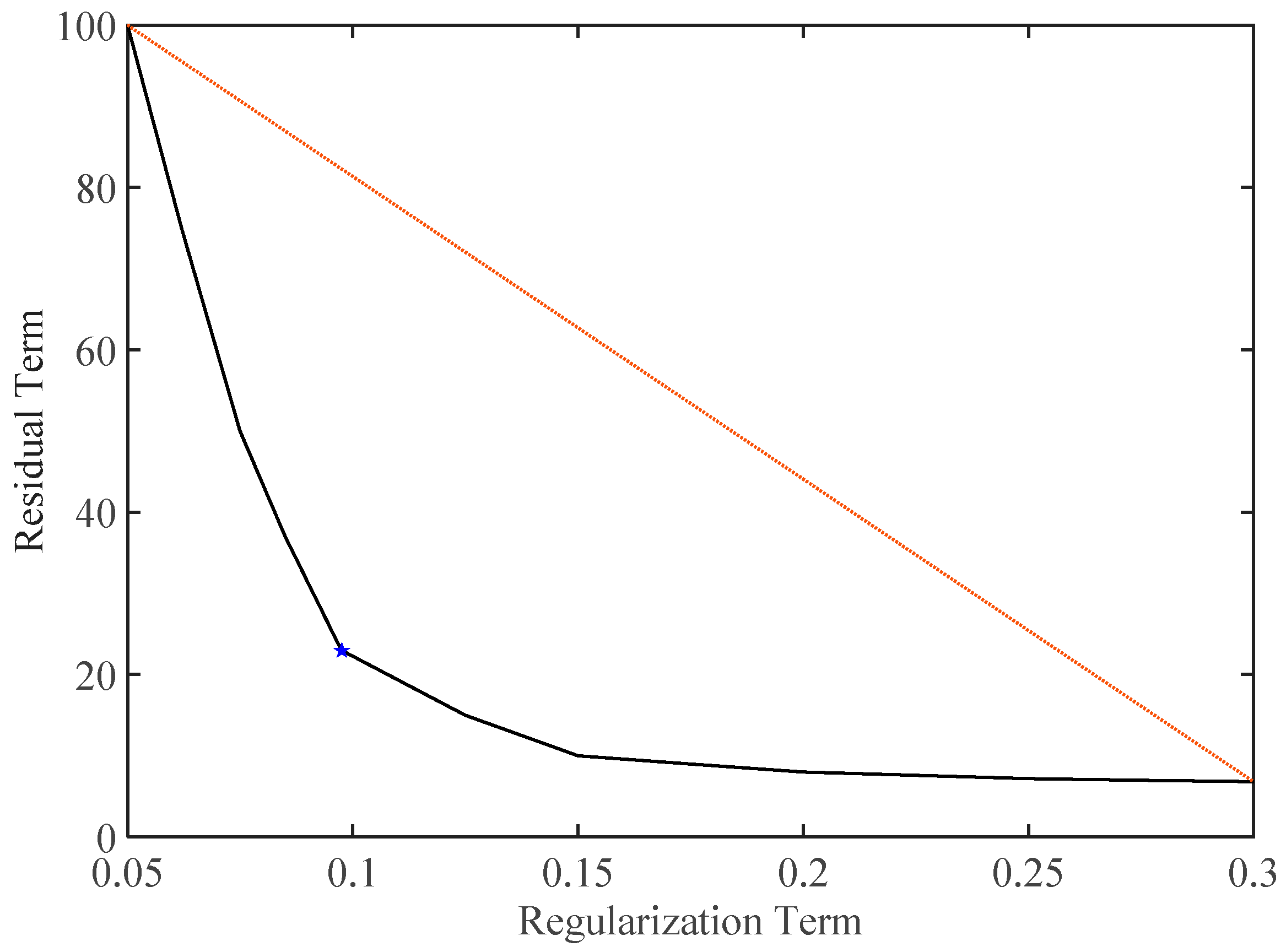
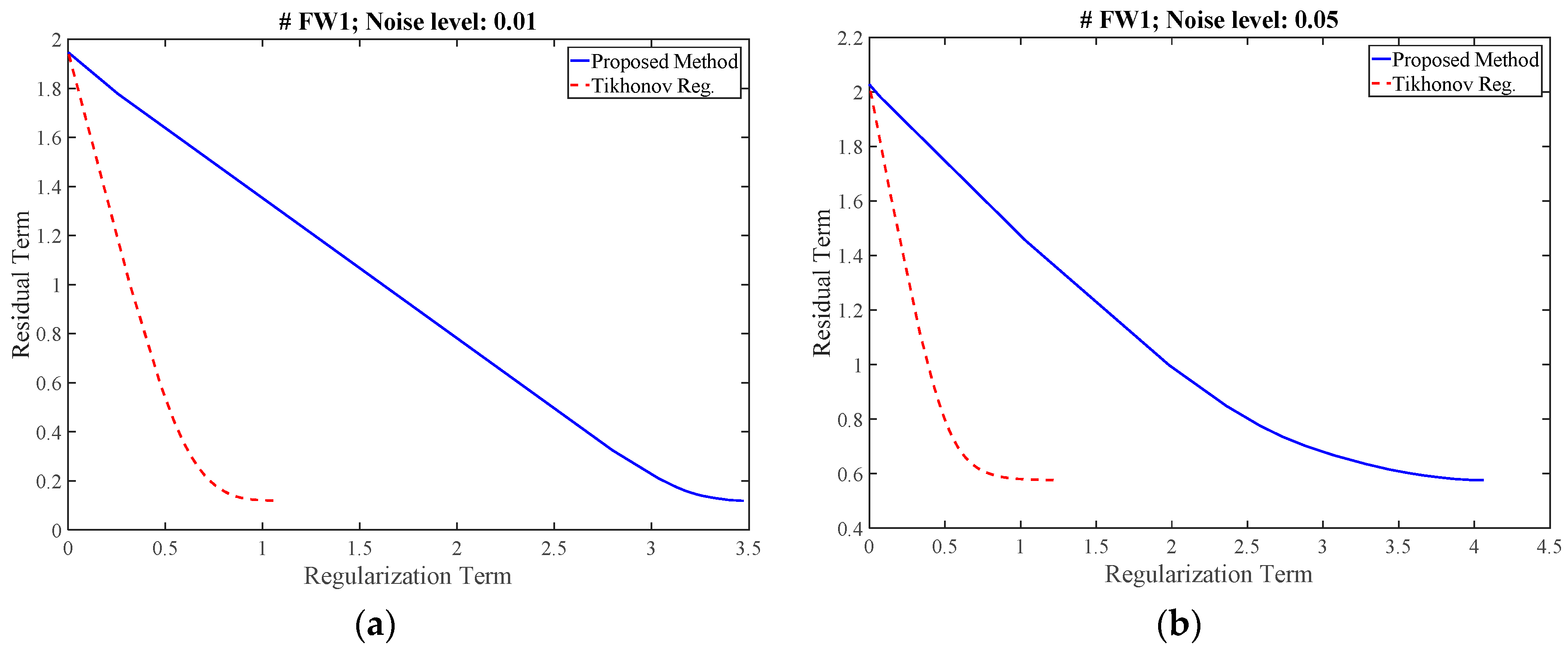
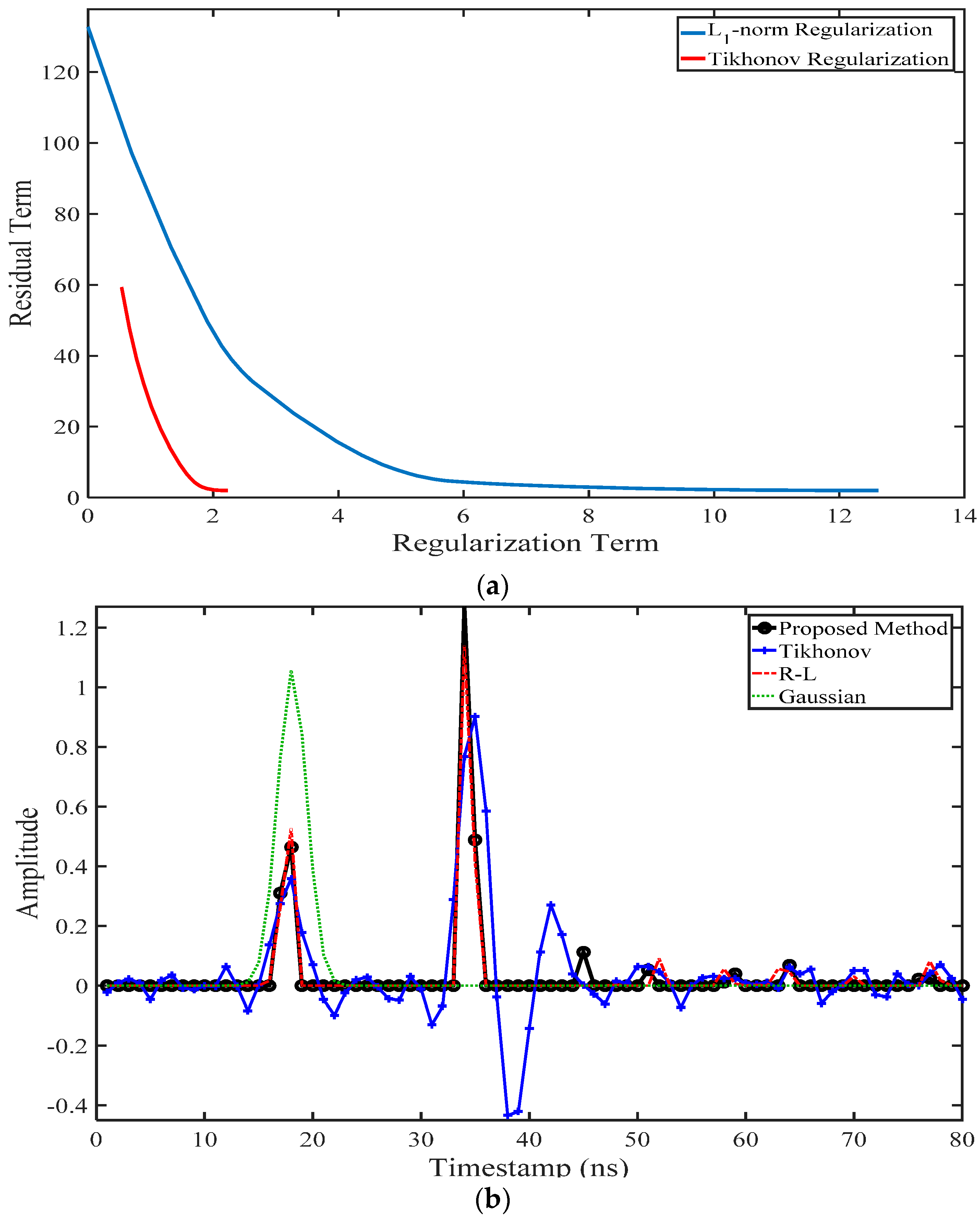
3.2. Determination of the Regularization Parameter

Optimal selection of the regularization parameter is important for an ideal adjustment between the regularization function and the solution residual, as the solution can be significantly affected by the selected value [35]. An optimal regularization parameter avoids under-/over-regularized results and in turn unreliable outputs. Therefore, a proper choice of the regularization parameter needs to be investigated thoroughly in order to achieve the optimal value.

Among the available approaches, some only deal with the residual term, without considering the regularization term. Of this type, the discrepancy principle [56] and generalized cross-validation (GCV) [57] could be mentioned. However, some other approaches, e.g., the L-curve [58], take care of both terms simultaneously [59].

The discrepancy principle method relies strictly upon a known data noise level and it estimates the regularization parameter such that the residual term is proportional to the predefined noise level [54,59]. The known noise level is considered as a highly impractical requirement when dealing with real data. Hansen et al. [54] highlighted an over-smoothed output yet with a known (or with a precise estimate of) noise level. Use of a large regularization parameter value makes the output signal over-smooth, and hence, the detailed description of the target response is not recovered [45,59]. These deficiencies make this approach inappropriate in the case of full-waveform lidar data processing.

Unlike the discrepancy principle, the GCV makes no assumption with regard to the noise level. The optimal value of the regularization parameter is obtained by minimizing the GCV function, where the effort is to achieve the minimal value of the residual term and eliminate the influence of small singular values on the output signal [54,59]. However, the occurrence of high correlation between noise elements impedes the achievement of an appropriate regularization parameter. Moreover, finding an absolute minimum value of the GCV function may not be achievable due to difficulty in locating the function’s minimum value since it is near constant in the vicinity of the minimum [45]. This method is also known for resulting in an overestimated regularization parameter, even in cases of unnoticeable correlation between errors. When it is applied to data with high noise level, results can be unsatisfactory [59].

In the L-curve method, both the residual and regularization terms are considered concurrently in order to find the optimal regularization parameter. In search of the optimal value, these two terms are plotted against each other for a range of plausible regularization parameter values. The idea is to find a changing point on the curve, where both terms are minimized simultaneously. This point is actually the margin between over- and under-regularization of the results and it is a representative of the optimal value for the regularization parameter [35]. The L-curve method is adopted for estimation of the optimal regularization parameter in this research in the following way: Suppose $P=\{(R{g}_1$, $R{s}_1),\dots ,\left(R{g}_n,R{s}_n\right)\}$ is a set of n pairs from the regularization ($R{g}_{\mathrm{i}}$) and residual term ($R{s}_{\mathrm{i}}$) magnitudes that constitute the vertices of the L-curve for a range of regularization parameter values (${\lambda }_1,{\lambda }_2,\dots ,{\lambda }_n$). The optimal regularization value ${\lambda }_{Opt}$ over the aforementioned set of points $P_i$ can then be conveniently calculated by finding the maximum Euclidean distance. Figure 1 illustrates the location of the optimal regularization parameter on a sample L-curve.

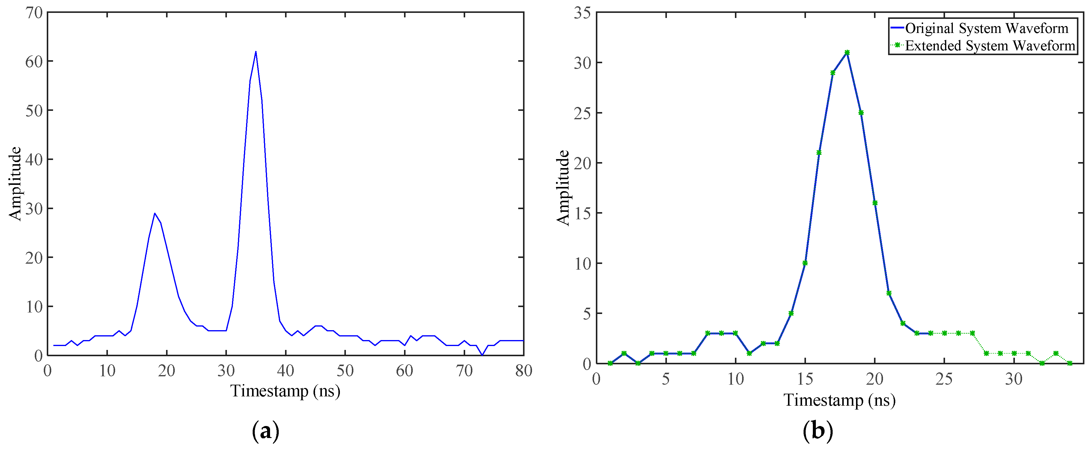
3.3. System Waveform Estimation

Waveform deconvolution requires the emitted signal to be known. This information is not always available in the recorded lidar data. In this section, a new method for estimation of the system waveform using blind deconvolution is proposed. Under the assumption of an ideally flat target (at nadir) and considering the measured transmitted signal $s_M\left(t\right)$ as a convolution of the transmitted pulse $s\left(t\right)$ and the impulse function of the transmitter $h_S\left(t\right)$ on one side; and assuming the measured received waveform $r_M\left(t\right)$ as a convolution of the transmitted pulse $s\left(t\right)$ and the receiver impulse function $h_R\left(t\right)$ on the other side; the measured received waveform can be expressed in the frequency domain as [24]:

$$R_M\left(f\right)=S_M\left(f\right)\frac{H_R\left(f\right)}{H_S\left(f\right)}=S_M\left(f\right)H\left(f\right)$$

(8)

The atmospheric propagation is treated as a constant value for similar targets located at similar ranges from the receiver. Therefore, the average of the system waveform can be obtained by deconvolution over a number of recorded samples. A prominent approach to eliciting a rough estimation of the unknown system waveform is to exploit blind deconvolution, which provides an estimate of both the point spread function (PSF) and the true signal [35,54]. In this research, only pulses captured at nadir over almost flat targets are taken into account for the calibration. In order to alleviate the effects of possible changes of the received waveforms from similar targets due to the noise, changes of the (unknown) system waveform or other unknown sources, the retrieved system waveforms are averaged. Estimation of the system waveform in this study is carried out using the iterative damped R-L method [60]. Once the system waveform is estimated, it will be applied to waveforms from other targets in order to achieve a rough estimate of the target cross-section via deconvolution. Possible changes in the system waveform, even between subsequent pulses, makes the retrieved target cross-section only a rough approximation.

3.4. Quantitative Assessment of the Retrieved Waveform

For quantitative comparison of the methods, the Fréchet distance, Spectral Angle Mapper (SAM), and Pearson correlation coefficient have been utilized to calculate the similarity of the results with the “true” cross-section signal.

The SAM metric measures the angle between two waveforms via treating them as vectors with identical lengths, and it can be expressed as follow:

$$\theta =co{s}^{-1}\left(\frac{{\sum }_{i=1}^{N}R{t}_{i}R{f}_i}{\sqrt{{\sum }_{i=1}^{N}R{t}_i^2{\sum }_{i=1}^{N}R{f}_i^2}}\right)$$

(9)

Here, $Rt$ and $Rf$ represent the retrieved and reference waveforms, respectively, where i and N are the index referring to the waveform samples and the total number of samples in a waveform.

The Pearson correlation coefficient r considers the linear relationship between the retrieved waveform $Rt$ and the reference signal $Rf$ in terms of the magnitude and direction:

$$r=\frac{S{S}_{Rt,Rf}^2}{S{S}_{Rt,Rt}S{S}_{Rf,Rf}}$$

(10)

where, $S{S}_{Rt,Rf}$ refers to the covariance of the waveforms, and $S{S}_{Rt,Rt}$ and $S{S}_{Rf,Rf}$ represent the standard deviations of each signal.

The Fréchet distance between $P:\left[a, b\right]\to {\text{ℝ}}^2$ and $Q:\left[a^{\prime },b^{\prime }\right]\to {\text{ℝ}}^2$ as two planar curves, with $d\left(P\left(\alpha \left(t\right)\right),Q\left(\beta \left(t\right)\right)\right)$ representing the Euclidean distance between these two curves at specified vertices, is defined as the minimum required length in connecting two separate paths, when navigating continuously from one endpoint to the other [61]:

$${\delta }_F\left(P,Q\right)=\underset{\alpha ,\beta }{inf}\underset{t\in \left[0,1\right]}{\max }d\left(P\left(\alpha \left(t\right)\right),Q\left(\beta \left(t\right)\right)\right)$$

(11)

where $a,b\in \text{ℝ}$ and a ≤ b (respectively $a^{\prime },b^{\prime }$), a (respectively β) is a function with continuous nondecreasing characteristics from [0, 1] onto $\left[a, b\right]$ (respectively $\left[a^{\prime },b^{\prime }\right]$), and $inf$(.) is the “infimum” or the maximum lower bound of a set.

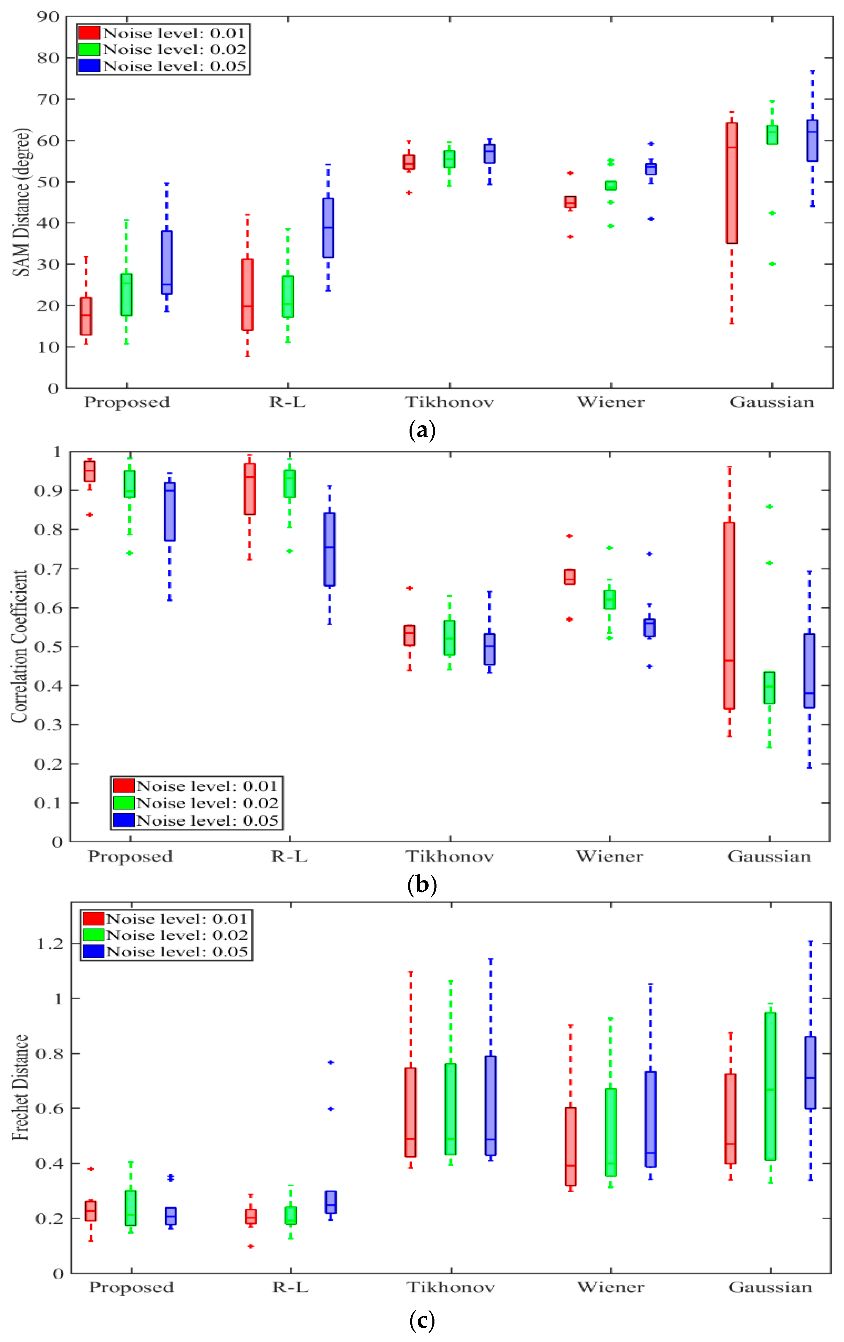
4. Experiments and Discussion

4.1. Experimental Data

A synthetic dataset and three different real datasets are investigated in order to evaluate the presented method.

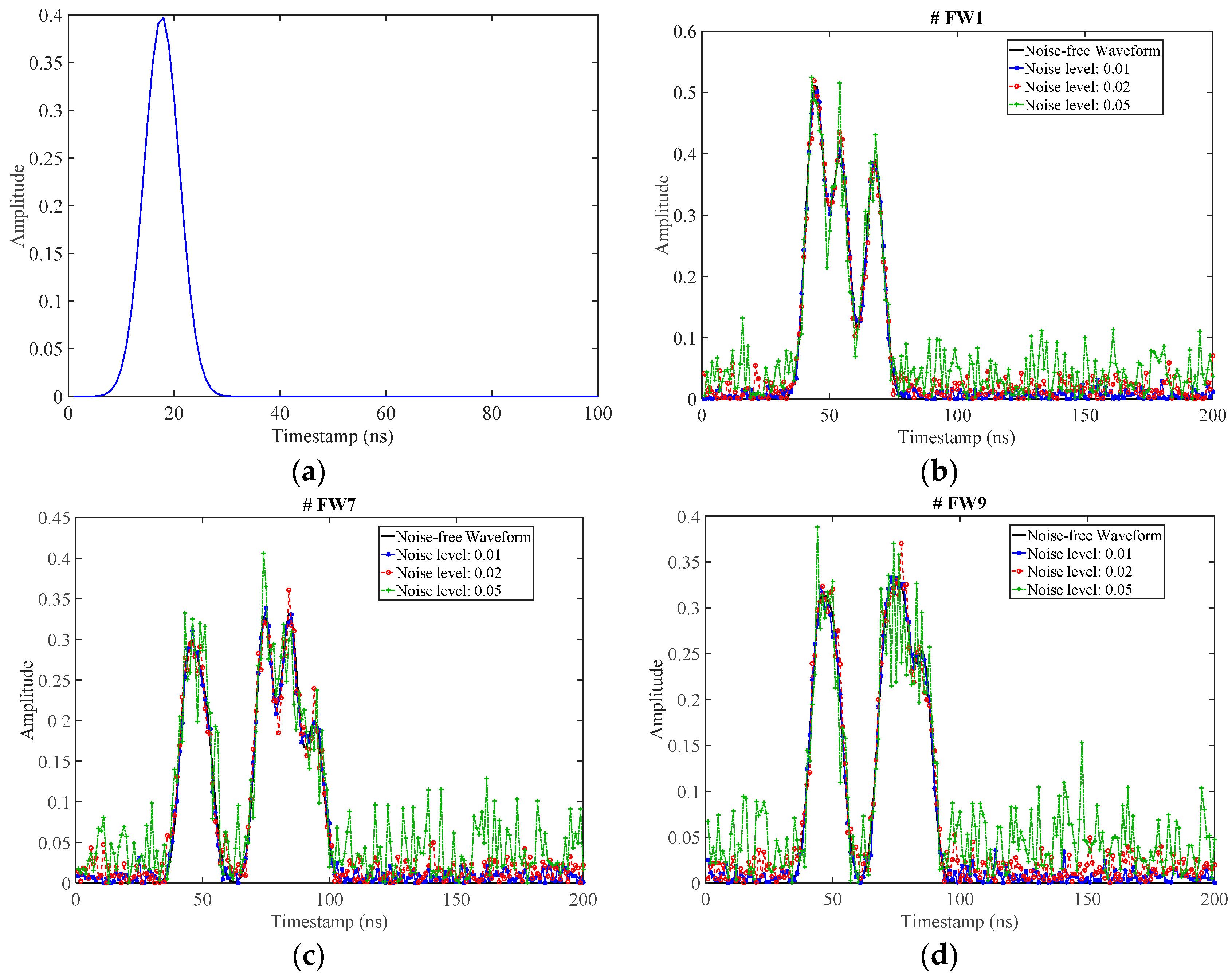
4.1.1. Synthetic Data

Ten synthetic lidar waveforms were generated by convolution of a known system signal and the given differential target cross-sections. For simplicity, all samples were considered as mixtures of samples with Gaussian distribution, with various levels of complexity and also different arrangements of pulses along the signals. This simulated data enables direct comparison of the restored waveform with the known “truth” data, facilitating quantitative evaluation of the performance of the deconvolution methods. Different arrangements of pulses with different amplitude values were considered so as to model different complexities of targets. In order to investigate the robustness of the methods against noise, the simulated signals were contaminated by three different noise levels (Gaussian noise with σ = 0.01, 0.02, and 0.05), after imposing a convolution with the synthetic system waveform. The absolute value of the amplitude values was utilized in order to avoid negative values resulted from the Gaussian noise. Figure 2 illustrates an example of both the synthetic system signal and the received waveforms at three different noise levels for limited samples. The true signals have been generated by computing the probability density functions based on the normal distribution, with different values assigned to the standard deviation to control the pulse shape.

4.1.2. Real LiDAR Datasets

Three different real datasets have been utilized to assess different aspects of the proposed method, including the approximation of the system waveform and the extraction of radiometric attributes for different targets. The QLD dataset was acquired over Rockhampton in Queensland, Australia, in December 2012. The NSW dataset was captured over the Namoi River in New South Wales, Australia in September 2013, and the third dataset was acquired over the Karawatha forest park in Queensland, Australia in October 2013. The laser footprint diameters at nadir were approximately 0.30 m, 0.50 m, and 0.15 m, respectively. A Riegl LMS-Q680i scanner, operating at 1550 nm, with the laser beam width of 0.5 mrad was used to acquire the datasets. Further details regarding the three lidar missions are provided in

Table 1. Data specification.

Parameter	QLD Dataset	NSW Dataset	Karawatha Dataset
Flying altitude (AGL-m)	600	1000	300
Pulse rate (kHz)	150	240	240
Maximal scan angle (°)	30	40	25

.

Although all datasets were recorded with the same instrument, the QLD data was provided without the system waveforms, while such information was delivered in the NSW and Karawatha data. With the latter two datasets, more satisfactory results are expected because of the recording of an equivalent system waveform for each received signal. Partial differences even between subsequent emitted pulses could then be observed.

As shown in Figure 3, the recorded system waveform in the NSW dataset was usually incomplete and there is no information at the signal tail. Interestingly, the maximum amplitude of the received waveform, shown in Figure 3, is higher than the value of the system waveform, which may seem contradictory. However, it is noticeable that amplitude values of the received waveform and the system waveform are not necessarily of identical units, which could be connected to the sampling procedure of the transmitted pulse [5]. The delayed backscattered energy due to multiple scattering within the tree crown is another possible explanation for this phenomenon.

The diversity of lidar datasets can present challenges in waveform deconvolution and thus the provision of the QLD, NSW and Karawatha datasets provided a good opportunity to evaluate the consistency of the proposed regularization method.

4.2. Preprocessing

The raw incoming waveform typically exhibits a certain level of noise due to sensor impacts and environment conditions. Moreover, deconvolution might amplify the noise due to its characteristics [31]. Therefore, a noise reduction method for full-waveform lidar based on the integration of the Savitzky-Golay (S-G) [62] and the Singular Value Decomposition (SVD) approaches was employed in the analysis [63]. This approach has advantages for signal pattern preservation, in addition to avoidance of waveform distortion.

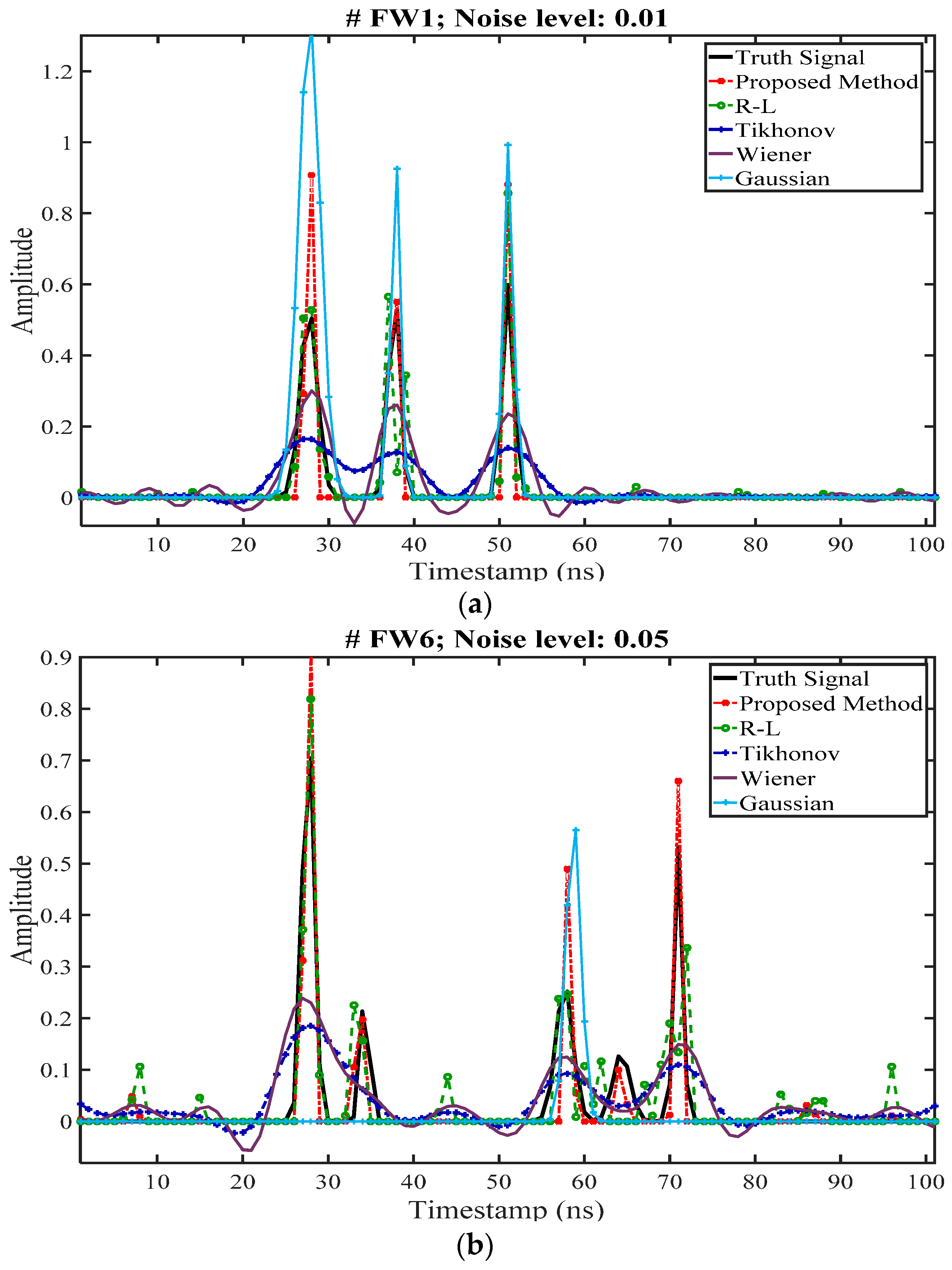
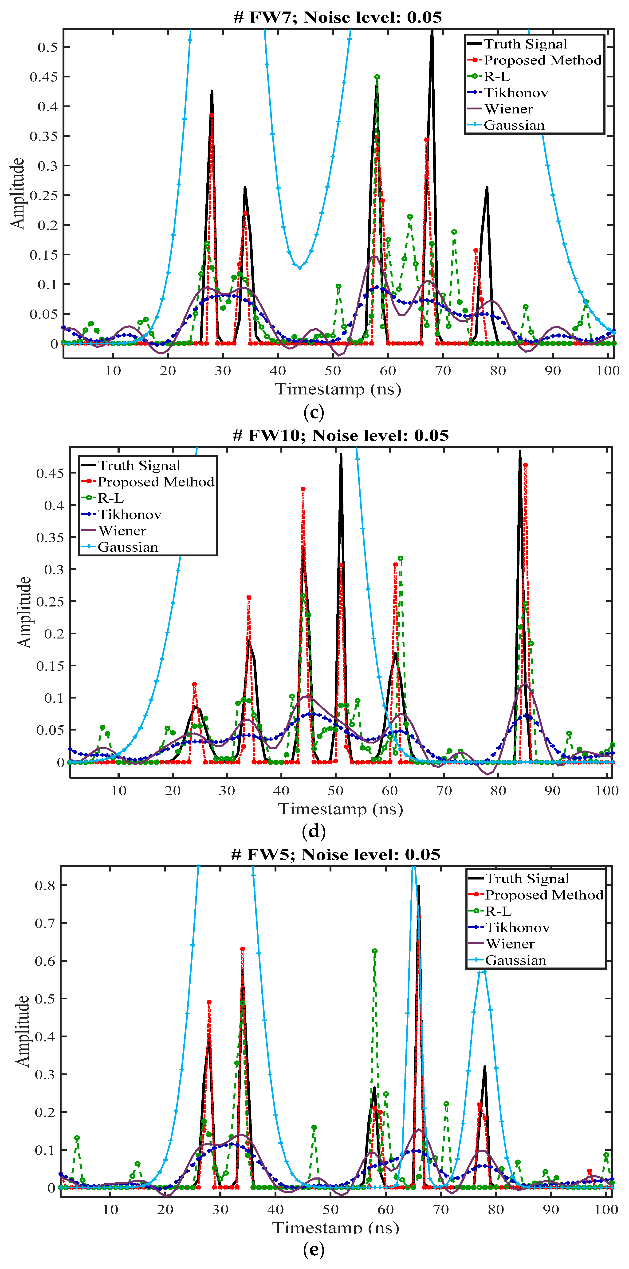
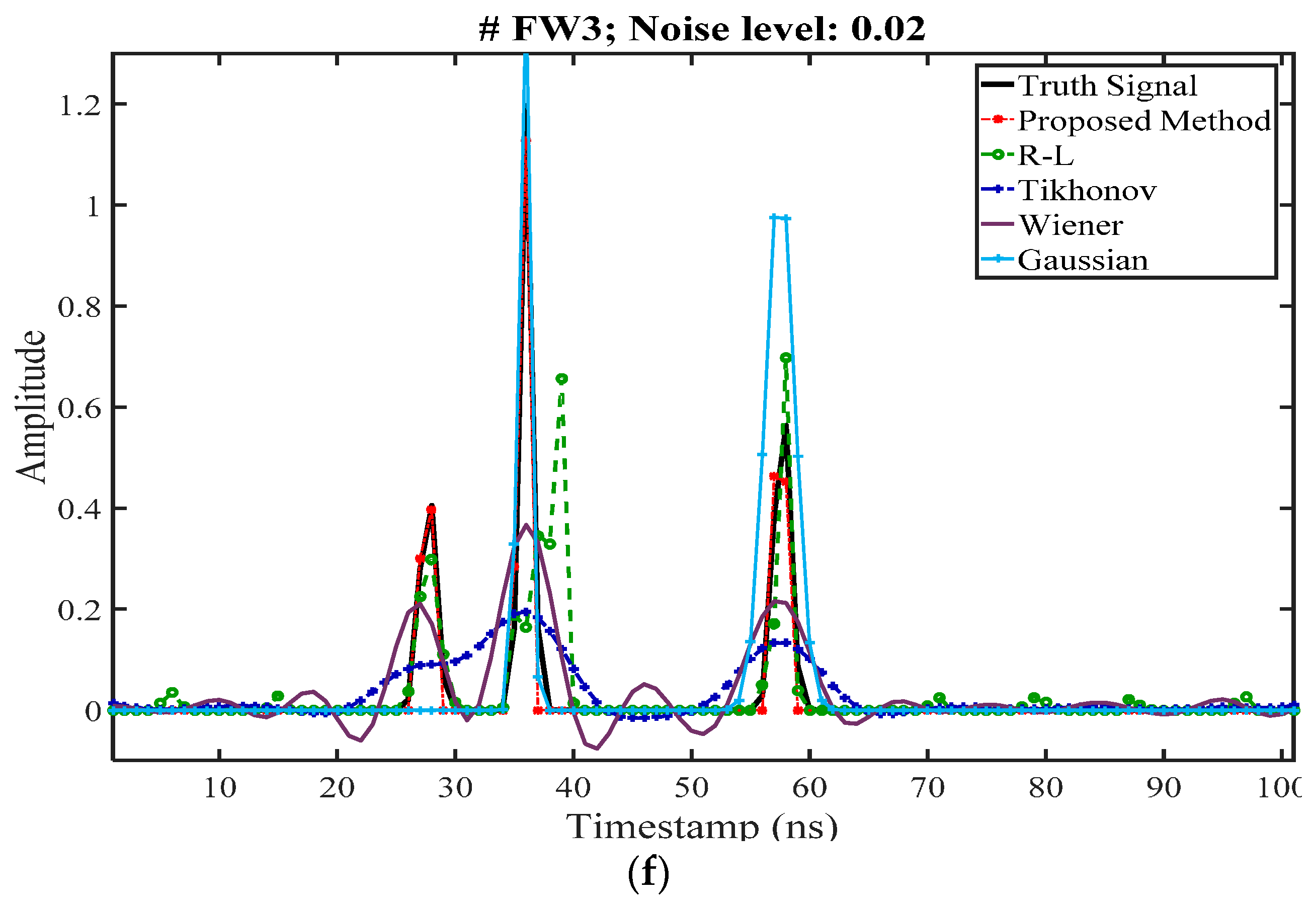
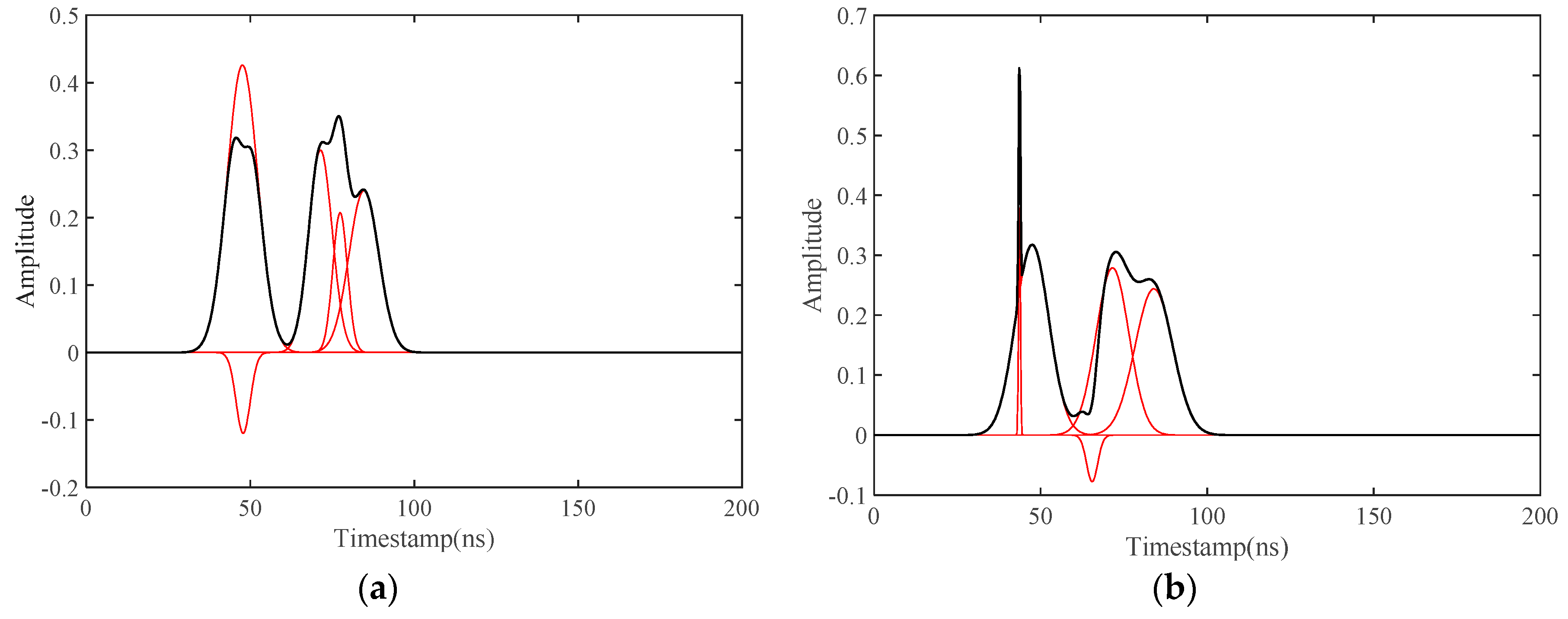
4.3. Deconvolution Results for Synthetic Waveforms

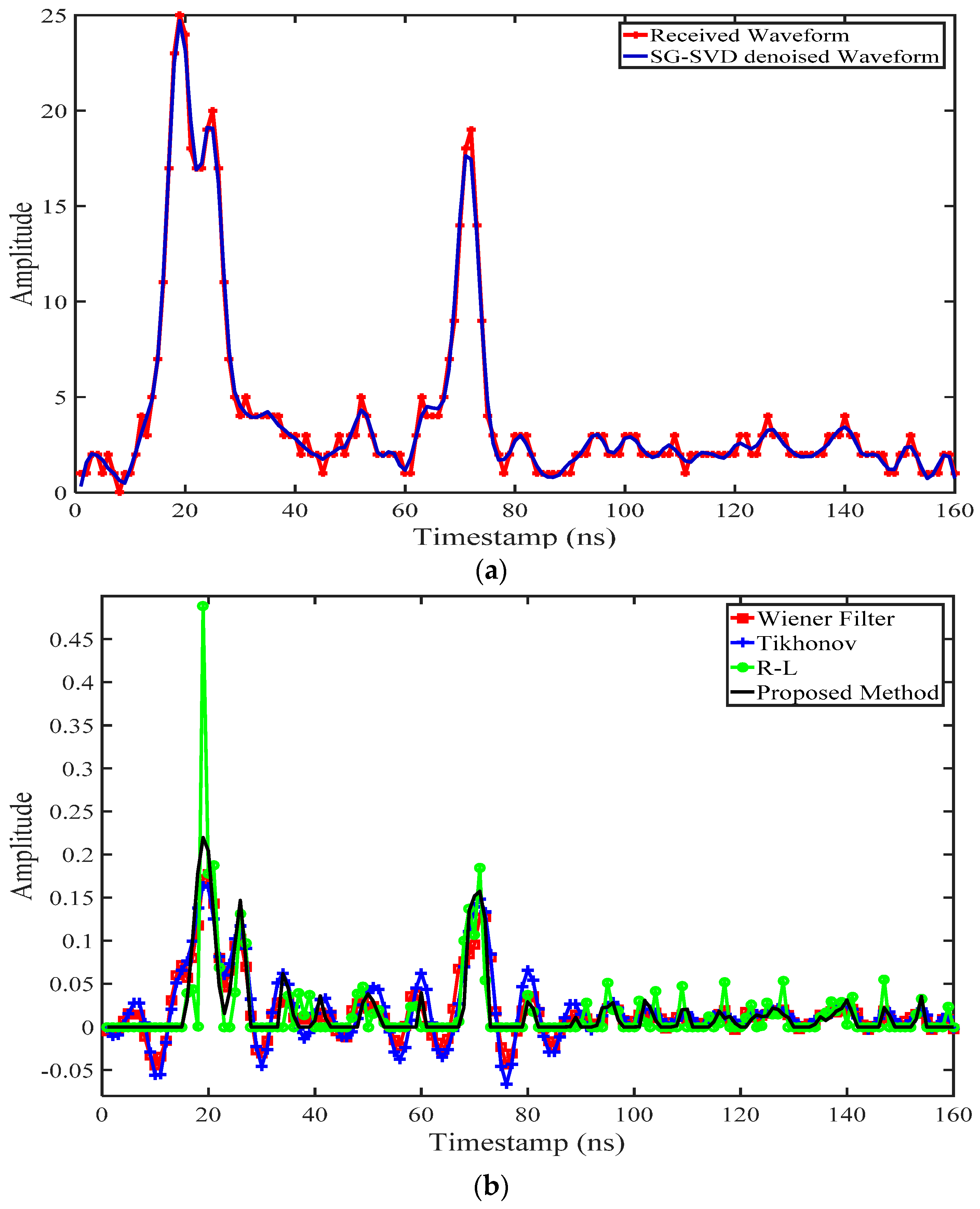
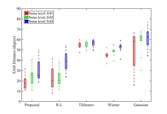
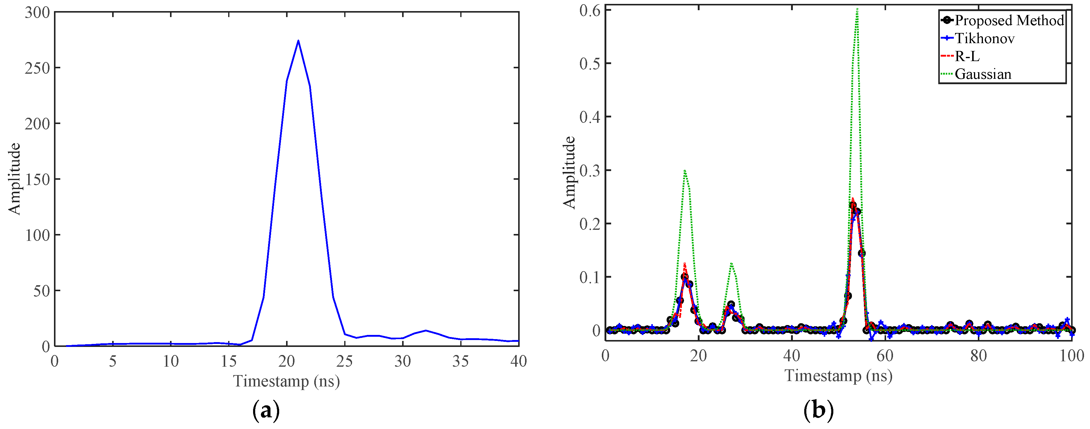
The synthetic data were processed by the proposed regularization approach and the results were compared to those from the commonly used approaches in signal processing, namely the R-L, Wiener filter, Tikhonov regularization, and Gaussian decomposition methods. The regularization parameter was determined by the L-curve method. The performance of the utilized approaches was quantitatively evaluated through a comparison of the estimated target cross-section with the “truth” data.

Table 2. Parameter tuning of the methods.

Method	Algorithm	Parameter Tuning	Reference(s)
Gaussian decomposition	Levenberg-Marquardt/Thrust region (curve fitting in Matlab)	Visual inspection to specify the number of pulses	[14,64]
R-L deconvolution	deconvlucy function in Matlab	RMSE criterion to select optimal iteration numbers	-
Wiener filtering	deconvwnr function in Matlab	$\frac{Noisevariance}{SignalVariance}$	-
Tikhonov regularization	CVX package	L-curve	[65,66]
Sparsity-based regularization	CVX package	L-curve	[65,66]

explains the parameter tuning for the methods, including the utilized algorithms and the associated references. The optimal iteration numbers of the R-L method were estimated by calculating the goodness of fit to the truth data by using the RMSE criterion, through consideration of a wide range of iteration numbers from 1 to 500. For the Wiener filter, the Noise to Signal Ratio (NSR) was calculated from the truth data at different noise levels by dividing the variance of the noise elements to the noise-free signal. Similar to the proposed deconvolution method, the regularization parameter was estimated by the L-curve method in the case of Tikhonov regularization. The exact number of expected pulses was assumed to be known in order to apply the Gaussian decomposition method through application of nonlinear optimization, e.g., the Levenberg-Marquardt algorithm [14].

Qualitative comparisons of the proposed method against the other four methods are shown in Figure 4 for selected samples. The figure provides a detailed evaluation of their performance in cases where the quantitative measures do not necessarily show a better performance of the proposed method. As shown in Figure 4a, qualitative inspection reveals the weakness of the R-L method in the retrieval of the second pulse, where two separate pulses are instead generated. Gaussian decomposition overestimates the amplitude for all three pulses, as well as the area under the first pulse, while the proposed method marginally overestimates two pulses. The Wiener filter and Tikhonov regularization methods generate oscillatory pulses that underestimate amplitude values of all pulses. In Figure 4b, the fourth pulse was not recovered by the R-L method, while the second and the last pulse were also shifted, with an underestimation of the last pulse as well. The proposed method retrieved all the pulses at their correct positions and with a minimum of spurious pulses. Gaussian decomposition only retrieves the third pulse which is marginally shifted. The second and fourth pulses were not retrieved by the Wiener and Tikhonov methods, while oscillation and underestimation of amplitude values were apparent. The last pulse was shifted by both the R-L and proposed methods in Figure 4c. Also, the R-L method could not retrieve the first two pulses and the fourth pulse, and many additional pulses were generated, probably as a result of noise amplification. The first two pulses and the last three pulses were combined separately in two pulses by the Gaussian decomposition, where the amplitude values were significantly overestimated. The Wiener filter performed slightly better in the retrieval of pulses than the Tikhonov method, yet the amplitude values were underestimated. In Figure 4d, the sixth pulse was marginally shifted by the proposed method, while the amplitudes of three other pulses were overestimated. The R-L method in this case cannot place the fourth pulse, while the first two pulses were not correctly restored in terms of both their amplitude and pulse locations. In addition, the last two pulses were slightly shifted and some other false pulses were generated. Two pulses were retrieved as combinations of the first four pulses by the Gaussian decomposition, where the amplitude values were overestimated. In Figure 4e, the first, fourth and fifth pulses were not restored by the R-L method, with spurious pulses instead being generated. The Gaussian decomposition method retrieved the last two pulses as well as a combination of the first two pulses, with the amplitudes being overestimated. Tikhonov and Wiener filtering resulted in both oscillations and underestimation of amplitude values for all pulses. In Figure 4f, the second pulse was not restored in its position using the R-L method. Gaussian decomposition, on the other hand, does not retrieve the first pulse, while the last pulse is overestimated in terms of both amplitude and the area under the pulse. The Wiener filter produces additional pulses, in addition to oscillation around the main peaks, whereas less spurious pulses were generated using the Tikhonov method. Even though the proposed method occasionally overestimates some of the pulses, the area under the curves were almost similar to the true signal.

It is noteworthy that the proposed method provides results of higher accuracy, retrieving all the peaks with minimal oscillations and minimum change in pulse position. By increasing the noise level to 0.05, better performance of the proposed method becomes more apparent, in comparison with the R-L method as the second best approach.

Figure 5 shows the comparison of the proposed method versus the R-L method, the Wiener filter, the Tikhonov regularization and Gaussian decomposition at three different noise levels based upon different quantitative metrics. Quantitatively, the accuracy of all methods is gradually diminished with increases in the noise level. According to the similarity metrics, shown in Figure 5, the proposed approach retrieves the synthetic target responses with higher accuracy in the majority of the cases. A slightly better performance is apparent for the R-L method at a σ value 0.02. However, the provided results of the R-L method are based on an ideal number of iterations related to the minimum RMSE against the true signals, which cannot be readily determined when dealing with real data.

As shown in Figure 5, Tikhonov regularization, Wiener filtering and Gaussian decomposition all provide signals with the lowest similarity to the truth waveforms. As seen in Figure 4, both Tikhonov regularization and the Wiener filter approaches result in ringing effects, with better separated pulses in the Wiener filter at the cost of revealing more spurious pulses and higher negative amplitude values. Both methods are deficient in regard to retrieval of the amplitude values and they both fail when dealing with complex waveforms and closely located pulses, with a higher level of pulse omission for the Tikhonov method. The inferior performance of Gaussian decomposition is mainly due to the inadequacy of the method in resolving closely located pulses. In addition, it generates pulses with negative amplitude values, as shown in Figure 6. Such pulses can be easily detected and removed from further processing, though at the cost of information deficiency. The poor performance of this method in the retrieval of the true signals is due to the smaller variance (pulse width) of the fitted pulse than the synthetic system waveform, which ultimately results in no solution for that pulse. The superior performance of the proposed method can be seen by looking at both the SAM distance and the correlation coefficient in Figure 5, while differences in terms of the Frechet distance are less noticeable.

Figure 7 shows the L-curves related to the l₁-norm and Tikhonov regularization methods. The L-curve provides an appropriate basis for determination of the optimal regularization parameter, which occurs at a balance point, thus demonstrating approximately reciprocal minimum values of both the residual and regularization terms. Although the optimal regularization parameter for solutions (at each noise levels) results in roughly similar residual norms (vertical axis), the solution magnitude (horizontal axis) is evidently larger in the case of the l₁-norm method at both noise levels. This implies that the solution amplitude can be retrieved with higher values closer to the true cross-section via the l₁-norm, and it confirms the underestimation of amplitude by the Tikhonov method. Overall, closer similarity to the truth data confirm the potential of the proposed method for retrieval of the cross-section signal.

4.4. QLD Dataset

The system waveform was not available in the QLD dataset. Due to its necessity for target cross-section retrieval, an estimation of the system waveform was provided by averaging the waveforms calculated from more than 500 waveform samples through applying blind deconvolution. The selected asphalt targets from which the system waveform was estimated have very gentle slopes of 2.4 degrees on average, at nadir. These small slope values cannot be considered as detrimental to the determination of the system waveform, since the pulse shapes are not distorted significantly by these gentle slopes. The averaged system waveform estimated based on blind deconvolution is shown in Figure 8a, where it was applied with the Gaussian decomposition, R-L method, the proposed method and Tikhonov deconvolution. Based on the USGS spectral library [67] for different types of asphalt, the reflectivity value of 0.2 proposed by Wagner et al. [14] was adopted since none of the values in the spectral library were more than 0.2 for the desired wavelength. Figure 8b shows the restored sample waveforms, where the first two returns are from a canopy and the last pulse belongs to a grass surface underneath.

The waveforms restored by the considered methods based on the estimated system waveforms from blind deconvolution were then examined, where prominent peaks are shown in all methods and marginal fluctuations were revealed in the restored signal in some cases.

From the restored signal, the target cross-section can be calculated. The overall target cross-section of the third pulse in Figure 8b, obtained simply by calculating the area under the pulse after applying the range correction [68], is 0.054 for the l₁-norm solution and 0.057 for the Tikhonov regularization method. These values are close to the equivalent value (0.071) obtained for a grass target with an approximate reflectivity of 0.25 [67] using Equation (1). The target cross-section estimates from Gaussian decomposition and the R-L methods were 0.082 and 0.046, respectively. This overestimation by Gaussian decomposition method is explained by the fact that such a function cannot describe all pulses appropriately. It is noticeable that the second pulse was not recovered when the number of expected pulses was set to three in the Gaussian decomposition. All three visible pulses could be restored by setting this value to four instead, while the restoration resulted in a null solution for the fourth pulse (located immediately after the third pulse).

Marginal underestimation of the total cross-section value by all methods, including the proposed method but excepting the case using Gaussian decomposition, can be attributed to either the footprint area being partially occluded by other targets (e.g., leaves) within the laser path which diminishes the transmitted pulse energy before it reaches the target, or to the approximated system waveform averaged over several samples. In addition, asphalt may not be ideally representative of a Lambertian target due to its variable optical characteristics [1]. Nevertheless, the experiment demonstrated the feasibility of blind deconvolution for estimation of the system waveform. This characteristic was confirmed in the NSW dataset where system waveforms were recorded.

4.5. NSW Dataset

The NSW dataset allowed further evaluation of the potential of the proposed approach in situations where the system waveform is recorded. Moreover, the availability of the system waveform provides an avenue to evaluate the proposed blind deconvolution approach. The effect of the L-curve method on the determination of regularization parameters can then be investigated and the performance of the proposed l₁-norm regularization approach can be compared to that of the other considered methods.

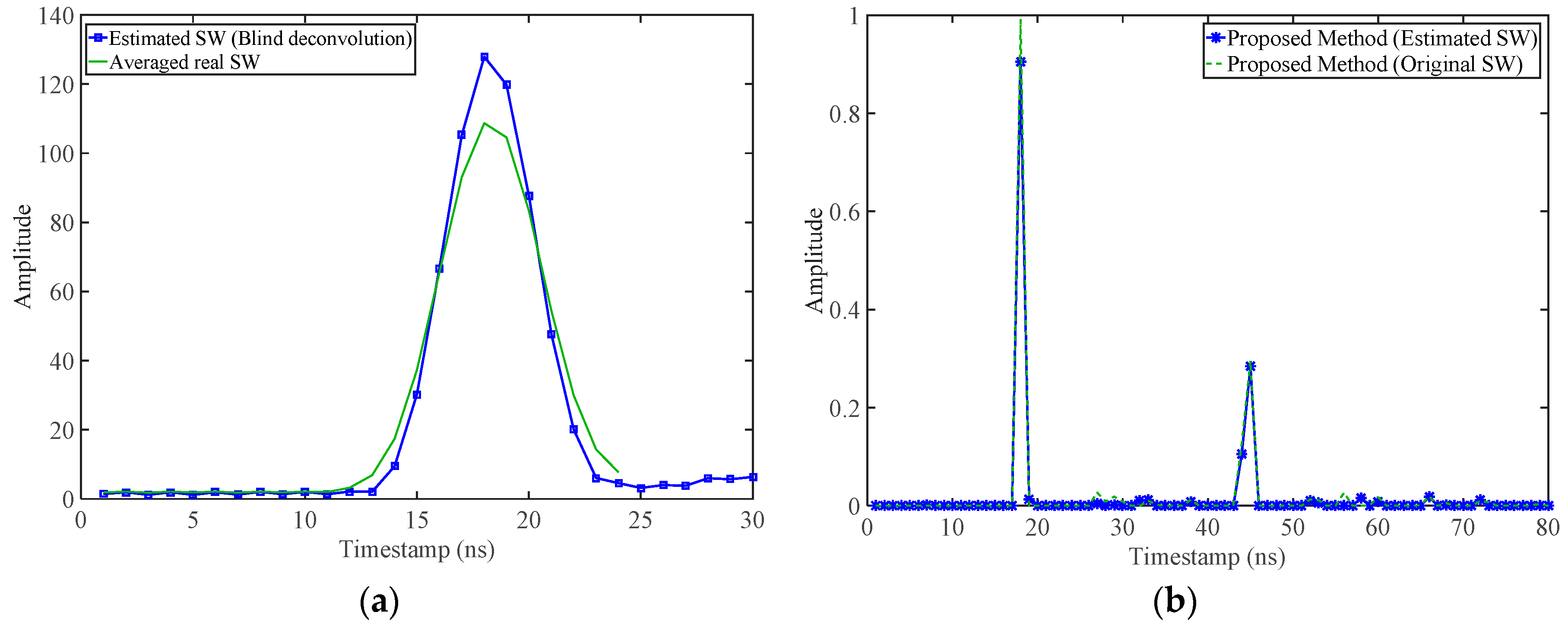
4.5.1. Evaluation of Blind Deconvolution for System Waveform Estimation

Over 4000 waveforms captured at nadir over non-asphalt flat targets were selected for the estimation of the system waveform, with the retrieved system waveform being plotted against the average of the recorded system waveforms in Figure 9a. The result shows that the shapes of both system waveforms are similar. The amplitude of the estimated waveform is slightly larger. This difference is explained by the fact that they are averaged over many samples, in which the arithmetic mean can be affected by extreme values. The SAM measure between the estimated and the averaged real waveforms is as small as 6.8 degrees. This result strongly supports the use of blind deconvolution for system waveform estimation when such information is not available. The retrieved temporal cross-section of a returned lidar waveform obtained using these two system waveforms in the proposed l₁-norm solution in the NSW dataset is shown in Figure 9b where similar amplitude values are seen in both pulses, through the first pulse is marginally underestimated when the estimated system waveform is adopted.

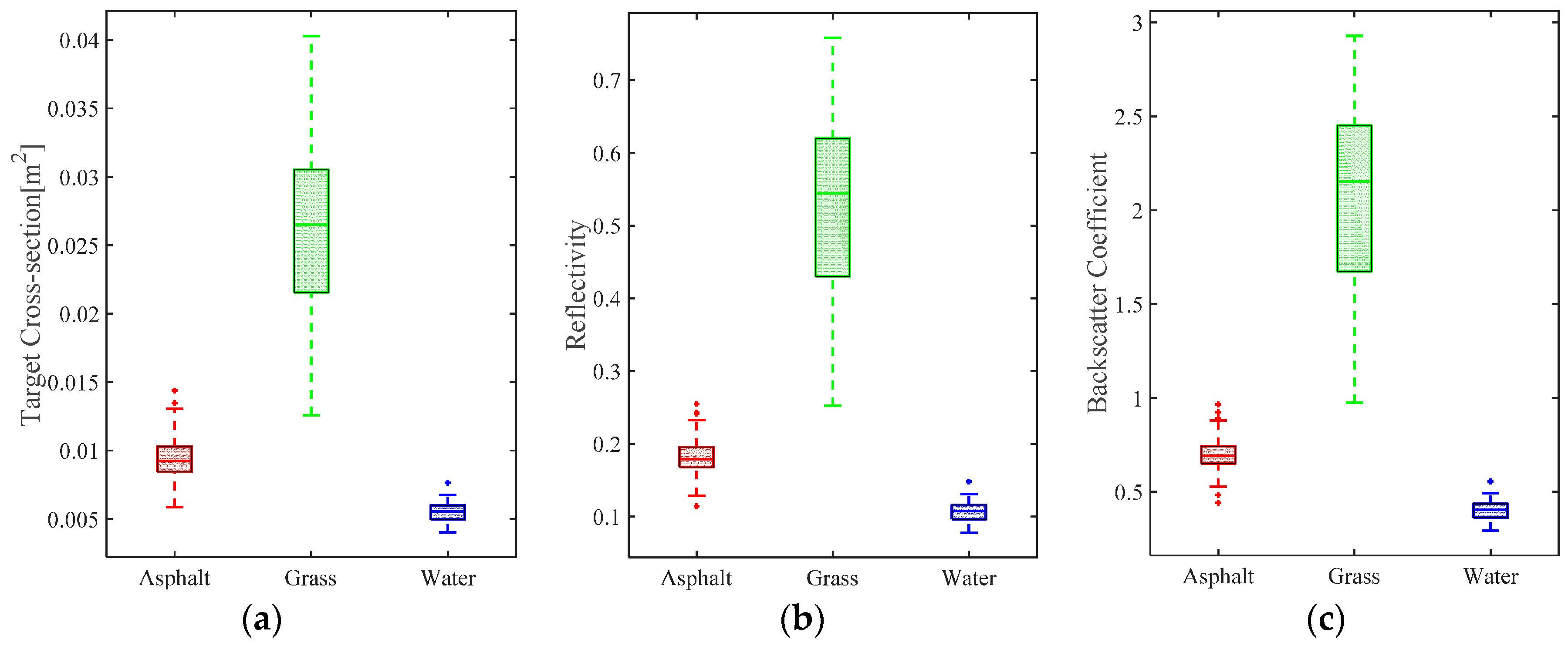
4.5.2. Target Cross-Section Recovery

Figure 10a illustrates the L-curve plots, which depict the associated magnitudes of the residual and the regularization terms for a range of expected regularization parameters of the waveform in Figure 3 for the l₁-norm and Tikhonov regularization approaches. As seen, the maximum magnitude of the regularization term (horizontal axis) in the proposed l₁-norm approach is larger than the magnitude of this term for Tikhonov regularization, implicitly confirming the potential of the former approach in the retrieval of a signal with higher amplitude values.

Larger regularization parameters for Tikhonov regularization (λ = 32.37) represent the placing of more emphasis on the regularization term and forcing the residual term to smaller values. Nevertheless, as shown in Figure 10b, the deconvolved signal was affected by noise and underestimation of the main amplitude values, together with fluctuations in between major amplitude values, which will occur as a consequence of the intrinsic characteristics of the l₂-norm, as well as smaller regularization terms, in comparison with the proposed l₁-norm solution. On the other hand, while a smaller regularization parameter for the l₁-norm method (λ = 15.26) indicates less emphasis on the regularization term, it allows the regularization magnitude to reach higher amplitude values. The deconvolved signal with the l₁-norm reveals the least artifacts or oscillations, especially around the main peaks.

Even though the nonlinear optimization results in the desired parameters for both pulses, Gaussian decomposition fails to retrieve the second pulse, mainly due to the smaller pulse width (variance) of the fitted function than that of the system waveform. This example clearly shows the deficiency of such a method in the retrieval of the target cross-section, even for pulses that are clearly separated. The R-L method results in a signal similar to that of the proposed method, when marginal over-/under-estimation of the pulses is evident.

Figure 11 presents a complex lidar waveform in the NSW dataset. The lidar signal penetrated through the tree canopy before reaching the ground, producing multiple peaks with varying amplitudes. The effect of multiple scattering reduces the strength of the pulses and causes delay in the returns, resulting in a long tail in the received waveform. The result of the implemented denoising approach in Azadbakht et al. [63], on the received waveform, is illustrated in Figure 11a.

The restored signals using the proposed l₁-norm method in comparison with those from the Tikhonov, Wiener and R-L approaches using the recorded system waveform are presented in Figure 11b. The l₁-norm regularization reveals all the peaks with no oscillation or negative amplitude. In the l₁-norm solution, small amplitude values between the main pulses, and after the ground return (last pulse), can be related to tree leaves and branches. The weak signals may be attributed to multiple scattering of tree foliage or to noise. Spikey-like pulses emerge in the case of the R-L approach, as the closest approach to the l₁-norm method in terms of cross-section retrieval, probably as a result of noise amplification. This confirms the vulnerability of the R-L method illustrated earlier using the synthetic dataset (Section 4.3). In comparison to all other methods, the R-L method produces a significantly overestimated amplitude for the first pulse. The largest oscillation and negative amplitudes in the restored waveforms are associated with the Tikhonov method, due to the inherent properties of the l₂-norm solution. Next is the Wiener filter with slightly smaller estimated amplitude values in addition to oscillation. In Figure 11, none of the pulses were retrieved using Gaussian decomposition, principally due to the system waveform being wider than the fitted Gaussian pulses in the received waveform. This method could also not fit a pulse to the second return when three pulses were considered as an initial value for the nonlinear optimization problem.

4.6. Karawatha Dataset

The target cross-section, the reflectance and the backscatter coefficient [15] of three types of extended non-overlapping targets were calculated, after retrieval of the temporal cross-sections and application of further required corrections [68]. Samples were collected over a range of scan angles from nadir to 25 degrees by inspecting points in a high resolution aerial photograph, taken simultaneously. Except for water bodies that were only available at limited scan angles, a total of around 200 samples were collected for each target.

Diffuse target reflectance behaviour was assumed in the calculation of the radiometric features, although this assumption is not valid for some targets, e.g., water bodies. However, relatively small reflectance values are due to the low strength of the received signal at off-nadir, for instance in the case of water bodies with specular reflectance characteristics. The provided results from the boxplots in Figure 12 confirm the reliability and relevance of the proposed approach in lidar waveform restoration. These targets can be readily distinguished only by using the radiometric information, while their height is almost similar and, therefore, geometric attributes are not effective.

5. Conclusions

This paper has presented a new deconvolution approach for efficient target cross-section extraction from full-waveform lidar data. The deconvolution, which removes the lidar system signal from the returned waveform and reconstructs the target cross-section independently of the instrument, is achieved through a versatile regularization approach with sparsity constraints, which copes with different kinds of waveforms. The regularization parameter, a critical issue in deconvolution, is determined with the L-curve method in which the optimal parameter is found at the turning point of the curve. Blind deconvolution is proposed to estimate the system signal, which is necessary on lidar instruments that do not record the system waveform.

The proposed approach has been evaluated using both synthetic and real lidar datasets acquired with and without system waveforms. While the synthetic data allowed for evaluation with “true” target cross-section, the real data provided an avenue to assess the consistency of the proposed approach under different instrument and environmental conditions. The results with synthetic data showed that the l₁-norm regularization, with the regularization parameter derived by the L-curve method, is superior to Tikhonov regularization, the Wiener filter, Gaussian decomposition and the R-L methods, which currently attract wide usage in lidar signal processing. The restored waveforms are strongly similar to the truth data despite the interference of different noise levels (Section 4.3).

The effectiveness of the proposed deconvolution method has been further demonstrated in experimental testing with real data, with and without system signals. It has been shown that the l₁-norm approach always results in a deconvolved signal almost free of substantial oscillations and negative amplitude values, while such phenomena are usually present with other approaches. Taken together, the findings of this study support adoption of sparse regularization as a means to retrieve the target response from full-waveform lidar.

The L-curve method has been shown to be reliable in the determination of the regularization parameter, as demonstrated in the experiments with both synthetic and real data.

Another finding to emerge from this research is that blind deconvolution has been demonstrated to be useful in the estimation of the system waveform when it is not available. Comparisons between the restored lidar waveforms using the system waveform based on blind deconvolution has been reported. Although restoration of the exact target response is not anticipated, due to the approximate estimation of the system waveform by averaging over several selected samples, the results demonstrate the consistency of the reported method in retrieving all pulses. Moreover, investigation of the blind deconvolution in the NSW dataset showed that the retrieved system waveform is in close agreement with the average system waveform of more than 3000 waveform samples. These visual and qualitative assessments indicate the significance of blind deconvolution in the retrieval of the system waveform, and they confirm that the deconvolved signal is associated with the target cross-section.

It is concluded that the proposed regularization approach can efficiently process full-waveform lidar data to restore the target cross-section. The use of this approach will provide additional insight into the waveform data. The restored cross-section affords the potential identification of either desired reflecting surfaces or even specific targets in a more consistent manner than is achieved with other approaches, thus improving the accuracy of range measurement and target attribute retrieval.

Future research will concentrate on investigation of the extracted geometric and radiometric features using the proposed method, along with additional potential attributes from the restored signal. Moreover, since direct regularization methods support inclusion of new constraints to better control the solution, investigation of additional term(s) in the objective function may result in even higher accuracy.

References

1. Mallet, C.; Bretar, F.; Roux, M.; Soergel, U.; Heipke, C. Relevance assessment of full-waveform lidar data for urban area classification. ISPRS J. Photogramm. Remote Sens. 2011, 66, S71–S84. [Google Scholar] [CrossRef]
2. Bretar, F.; Chauve, A.; Mallet, C.; Jacome, A. Terrain surfaces and 3-D landcover classification from small footprint full-waveform lidar data: Application to badlands. Hydrol. Earth Syst. Sci. 2009, 13, 1531–1545. [Google Scholar] [CrossRef]
3. Jutzi, B.; Stilla, U. Extraction of features from objects in urban areas using spacetime analysis of recorded laser pulses. Int. Arch. Photogramm. Remote Sens. Spat. Inf. Sci. 2004, 35, 1–6. [Google Scholar]
4. Hovi, A.; Korpela, I. Real and simulated waveform-recording LiDAR data in juvenile boreal forest vegetation. Remote Sens. Environ. 2014, 140, 665–678. [Google Scholar] [CrossRef]
5. Adams, T.; Beets, P.; Parrish, C. Extracting more data from lidar in forested areas by analyzing waveform shape. Remote Sens. 2012, 4, 682–702. [Google Scholar] [CrossRef]
6. Hollaus, M.; Aubrecht, C.; Höfle, B.; Steinnocher, K.; Wagner, W. Roughness mapping on various vertical scales based on full-waveform airborne laser scanning data. Remote Sens. 2011, 3, 503–523. [Google Scholar] [CrossRef]
7. Mallet, C.; Bretar, F. Full-waveform topographic lidar: State-of-the-art. ISPRS J. Photogramm. Remote Sens. 2009, 64, 1–16. [Google Scholar] [CrossRef]
8. Höfle, B.; Pfeifer, N. Correction of laser scanning intensity data: Data and model-driven approaches. ISPRS J. Photogramm. Remote Sens. 2007, 62, 415–433. [Google Scholar] [CrossRef]
9. Jutzi, B.; Stilla, U. Laser pulse analysis for reconstruction and classification of urban objects. In Proceedings of the International Society Photogrammetry and Remote Sensing (ISPRS) Archives, Munich, Germany, 17–19 September 2003.
10. Wagner, W.; Ullrich, A.; Melzer, T.; Briese, C.; Kraus, K. From single-pulse to full-waveform airborne laser scanners: Potential and practical challenges. Int. Arch. Photogram. Remote Sens. 2004, 35, 201–206. [Google Scholar]
11. Roncat, A.; Bergauer, G.; Pfeifer, N. B-spline deconvolution for differential target cross-section determination in full-waveform laser scanning data. ISPRS J. Photogramm. Remote Sens. 2011, 66, 418–428. [Google Scholar] [CrossRef]
12. Jutzi, B.; Stilla, U. Range determination with waveform recording laser systems using a Wiener Filter. ISPRS J. Photogramm. Remote Sens. 2006, 61, 95–107. [Google Scholar] [CrossRef]
13. Jelalian, A.V. Laser Radar Systems; Artech House: Boston, MA, USA; London, UK, 1992. [Google Scholar]
14. Wagner, W.; Ullrich, A.; Ducic, V.; Melzer, T.; Studnicka, N. Gaussian decomposition and calibration of a novel small-footprint full-waveform digitising airborne laser scanner. ISPRS J. Photogramm. Remote Sens. 2006, 60, 100–112. [Google Scholar] [CrossRef]
15. Wagner, W. Radiometric calibration of small-footprint full-waveform airborne laser scanner measurements: Basic physical concepts. ISPRS J. Photogramm. Remote Sens. 2010, 65, 505–513. [Google Scholar] [CrossRef]
16. Wang, Y.; Zhang, J.; Roncat, A.; Künzer, C.; Wagner, W. Regularizing method for the determination of the backscatter cross section in lidar data signals. Opt. Soc. Am. 2009, 26, 1071–1079. [Google Scholar] [CrossRef]
17. Chauve, A.; Vega, C.; Durrieu, S.; Bretar, F.; Allouis, T.; Deseilligny, M.P.; Puech, W. Advanced full-waveform lidar data echo detection: Assessing quality of derived terrain and tree height models in an alpine coniferous forest. Int. J. Remote Sens. 2009, 30, 5211–5228. [Google Scholar] [CrossRef]
18. Lin, Y.-C.; Mills, J.P.; Smith-Voysey, S. Rigorous pulse detection from full-waveform airborne laser scanning data. Int. J. Remote Sens. 2010, 31, 1303–1324. [Google Scholar] [CrossRef]
19. Parrish, C.E.; Jeong, I.; Nowak, R.D.; Smith, R.B. Empirical Comparison of Full-Waveform Lidar Algorithms: Range Extraction and Discrimination Performance. Photogram. Eng. Remote Sens. 2011, 77, 825–838. [Google Scholar] [CrossRef]
20. Wu, J.; Aardt, J.A.N.V.; Asner, G.P. A comparison of signal deconvolution algorithms based on small-footprint lidar waveform simulation. IEEE Trans. Geosci. Remote Sens. 2011, 49, 2402–2414. [Google Scholar] [CrossRef]
21. Hofton, M.A.; Minster, J.B.; Blair, J.B. Decomposition of Laser Altimeter Waveforms. IEEE Trans. Geosci. Remote Sens. 2000, 38, 1989–1996. [Google Scholar] [CrossRef]
22. Persson, A.; Söderman, U.; Töpel, J.; Ahlberg, S. Visualization and analysis of full-waveform airborne laser scanner data. In Proceedings of the ISPRS Workshop Laser Scanning, Enschede, The Netherlands, 12–14 September 2005; pp. 103–108.
23. Mallet, C.; Lafarge, F.; Roux, M.; Soergel, U.; Bretar, F.; Heipke, C. A marked point process for modeling lidar waveforms. IEEE Trans. Image Process. 2010, 19, 3204–3221. [Google Scholar] [CrossRef] [PubMed] [Green Version]
24. Jutzi, B.; Stilla, U. Characteristics of the measurement unit of a full-waveform laser system. Int. Arch. Photogramm. Remote Sens. Spat. Inf. Sci. 2006, 36, 17–22. [Google Scholar]
25. Alexander, C.; Tansey, K.; Kaduk, J.; Holland, D.; Tate, N.J. Backscatter coefficient as an attribute for the classification of full-waveform airborne laser scanning data in urban areas. ISPRS J. Photogramm. Remote Sens. 2010, 65, 423–432. [Google Scholar] [CrossRef]
26. Zhu, R.; Pang, Y.; Zhang, Z.; Xu, G. Application of the deconvolution method in the processing of full-waveform LiDAR data. In Proceedings of the 3rd International Congress on Image and Signal Processing (CISP2010), Yantai, China, 16–18 October 2010; pp. 2975–2979.
27. Chauve, A.; Mallet, C.; Bretar, F.; Durrieu, S.; Deseilligny, M.P.; Puech, W. Processing full-waveform lidar data: Modelling raw signals. In Proceedings of the ISPRS Workshop on Laser Scanning 2007 and SilviLaser 2007, Espoo, Finland, 12–14 September 2007; pp. 102–107.
28. Wu, J.; van Aardt, J.A.N.; McGlinchy, J.; Asner, G.P. A robust signal preprocessing chain for small-footprint waveform lidar. IEEE Trans. Geosci. Remote Sens. 2012, 50, 3242–3255. [Google Scholar] [CrossRef]
29. Reeves, S. Generalized cross-validation as a stopping rule for the Richardson-Lucy algorithm. Int. J. Imaging Syst. Technol. 1995, 6, 387–391. [Google Scholar] [CrossRef]
30. Khan, M.K.; Morigi, S.; Reichel, L.; Sgallari, F. Iterative methods of richardson-lucy-type for image debluring. Numer. Math. Theory Methods Appl. 2013, 6, 262–275. [Google Scholar]
31. Neilsen, K.D. Signal Processing on Digitized LADAR Waveforms for Enhanced Resolution on Surface Edges. Master’s Thesis, Utah State University, Logan, UT, USA, 2011. [Google Scholar]
32. Morháč, M.; Matoušek, V. High-resolution boosted deconvolution of spectroscopic data. J. Comput. Appl. Math. 2011, 235, 1629–1640. [Google Scholar] [CrossRef]
33. Castorena, J.; Creusere, C.D.; Voelz, D. Modeling LiDAR scene sparsity using compressicve sensing. In Proceedings of the 2010 IEEE International Geoscience and Remote Sensing Symposium (IGARSS), Honolulu, HI, USA, 25–30 July 2010.
34. Verdin, B.; von Borries, R. Lidar compressive sensing using chaotic waveform. Proc. SPIE Radar Sens. Technol. 2014. [Google Scholar] [CrossRef]
35. Gunturk, B.K. Fundamentals of image restoration. In Image Restoration: Fundamentals and Advances; Gunturk, B.K., Li, X., Eds.; CRC Press: Boca Raton, FL, USA, 2012; pp. 25–61. [Google Scholar]
36. Gold, R. An Iterative Unfolding Method for Response Matrices; Argonne National Laboratory: Argonne, IL, USA, 1964. [Google Scholar]
37. Richardson, W.H. Bayesian-based iterative method of image restoration. J. Opt. Soc. Am. 1972, 62, 55–59. [Google Scholar] [CrossRef]
38. Lucy, L.B. An iterative method for the rectification of the observed distributions. Astron. J. 1974, 79, 745–754. [Google Scholar] [CrossRef]
39. Vogel, C.R. Computational Methods for Inverse Problems; Frontiers in Applied Mathematics Series; Society of Industrial and Applied Mathematics (SIAM): Philadelphia, PA, USA, 2002; p. 183. [Google Scholar]
40. Stefan, W. Total Variation Regularization for Linear Ill-Posed Inverse Problems Extensions and Applications. Ph.D. Thesis, Arizona State University, Phoneix, AZ, USA, 2008. [Google Scholar]
41. Hansen, P.C. The discrete picard condition for discrete ill-posed problems. BIT Numer. Math. 1990, 30, 658–672. [Google Scholar] [CrossRef]
42. Boyd, S.; Vandenberghe, L. Convex Optimization; Cambridge University Press: New York, NY, USA, 2004; p. 727. [Google Scholar]
43. Tikhonov, A.N.; Arsenin, V.I.A. Solutions of Ill-Posed Problems; Winston & Sons: Washington, DC, USA, 1977; p. 258. [Google Scholar]
44. Elad, M.; Figueiredo, A.T.; Ma, Y. On the role of sparse and redundant representations in image processing. IEEE Proc. 2010, 98, 972–982. [Google Scholar] [CrossRef]
45. Hansen, P.C.; O’Leary, D.P. The use of the L-curve in the regularization of discrete ill-posed problems. SIAM J. Sci. Comput. 1993, 14, 1487–1503. [Google Scholar] [CrossRef]
46. Pan, T.C. Signal and Image Deconvolution: Algorithms and Applications. Ph.D. Thesis, Hong Kong Baptist University, Hong Kong, China, 2010. [Google Scholar]
47. Figueiredo, M.A.T.; Bioucas-Dias, J.M. Algorithms for imaging inverse problems under sparsity regularization. In Proceedings of the 3rd International Workshop on Cognitive Information Processing (CIP), Baiona, Spain, 28–30 May 2012; pp. 1–6.
48. Tropp, J.A.; Wright, S.J. Computational methods for sparse solution of linear inverse problems. IEEE Proc. 2010, 98, 948–958. [Google Scholar] [CrossRef]
49. Schmidt, M.; Fung, G.; Rosales, R. Fast optimization methods for L1 regularization: A comparative study and two new approaches. In Machine Learning: ECML 2007; Springer: Berlin, Germany; Heidelberg, Germany, 2007; pp. 286–297. [Google Scholar]
50. Kim, S.-J.; Koh, K.; Lustig, M.; Boyd, S.; Gorinevsky, D. An interior-point method for large-scale l1-regularized least squares. IEEE J. Sel. Top. Signal Proc. 2007, 1, 606–617. [Google Scholar]
51. Palomar, D.P.; Eldar, Y.C. Convex Optimization in Signal Processing and Communications; Cambridge University Press: New York, NY, USA, 2010; p. 498. [Google Scholar]
52. Alizadeh, F.; Goldfarb, D. Second-order cone programming. Math. Program. 2003, 95, 3–51. [Google Scholar] [CrossRef]
53. Sousa, M.; Vandenberghe, L.; Boyd, S.; Lebret, H. Applications of second-order cone programming. Linear Algebra Appl. 1998, 284, 193–228. [Google Scholar]
54. Hansen, P.C.; Nagy, J.G.; O’Leary, D.P. Deblurring Images: Matrices, Spectra, and Filtering; Society of Industrial and Applied Mathematics (SIAM): Philadelphia, PA, USA, 2006; p. 130. [Google Scholar]
55. Orfanidis, S.J. Introduction to Signal Processing; Prentice Hall: Upper Saddle River, NJ, USA, 2010; p. 783. [Google Scholar]
56. Morozov, V.A. On the solution of functional equations by the method of regularization. Sov. Math. Dokl. 1966, 7, 414–417. [Google Scholar]
57. Golub, G.; Heath, M.; Wahba, G. Generalized cross-validation as a method for choosing a good ridge parameter. Technometrics 1979, 21, 215–223. [Google Scholar] [CrossRef]
58. Hansen, P.C. Analysis of discrete ill-posed problems by means of the L-curve. SIAM Rev. 1992, 34, 561–580. [Google Scholar] [CrossRef]
59. Correia, T.; Gibson, A.; Schweiger, M.; Hebden, J. Selection of regularization parameter for optical topography. J. Biomed. Opt. 2009, 14. [Google Scholar] [CrossRef] [PubMed]
60. White, R.L. Image restoration using the damped Richardson-Lucy method. In Proceedings of the SPIE 2198, Instrumentation in Astronomy VIII, Kailua-Kona, HI, USA, 13 March 1994; pp. 1342–1348.
61. Rote, G. Computing the Fréchet distance between piecewise smooth curves. Comput. Geom. 2007, 37, 162–174. [Google Scholar] [CrossRef]
62. Savitzky, A.; Golay, M.J.E. Smoothing and differentiation of data by simplified least squares procedures. Anal. Chem. 1964, 36, 1627–1639. [Google Scholar] [CrossRef]
63. Azadbakht, M.; Fraser, C.S.; Zhang, C.; Leach, J. A signal denoising method for full-waveform LiDAR data. In Proceedings of the ISPRS Annals of Photogrammetry, Remote Sensing and Spatial Information Sciences, Antalya, Turkey, 11–13 November 2013; pp. 31–36.
64. Roncat, A. Backscatter Signal Analysis of Small-Footprint Full-Waveform Lidar Data. Ph.D. Thesis, Vienna University of Technology, Vienna, Austria, 2014. [Google Scholar]
65. Grant, M.; Boyd, S. Graph implementations for nonsmooth convex programs. In Recent Advances in Learning and Control; Blondel, V.D., Boyd, S., Kimura, H., Eds.; Springer: London, UK, 2008; pp. 95–110. [Google Scholar]
66. Grant, M.; Boyd, S. CVX: Matlab Software for Disciplined Convex Programming. Available online: http://cvxr.com/cvx (accessed on 30 May 2016).
67. Clark, R.N.; Swayze, G.A.; Wise, R.A.; Livo, K.E.; Hoefen, T.M.; Kokaly, R.F.; Sutley, S.J. USGS Digital Spectral Library Splib06a. Available online: http://speclab.cr.usgs.gov/spectral.lib06/ds231/ (accessed on 20 September 2007).
68. Azadbakht, M.; Fraser, C.S.; Zhang, C. Separability of targets in urban areas using features from full-waveform LiDAR data. In Proceedings of the IEEE International Geoscience and Remote Sensing Symposium (IGARSS), Milan, Italy, 26–31 July 2015; pp. 5367–5370.
Figure 1. Optimal regularization parameter on the L-curve.
Remotesensing 08 00648 g001
Figure 2. (a) The synthetic system waveform; and (bd) selected sample waveforms at different noise levels.
Remotesensing 08 00648 g002
Figure 3. (a) A typical recorded waveform in the NSW dataset; and (b) its corresponding original system waveform.
Remotesensing 08 00648 g003
Figure 4. (af) Qualitative comparison of sample retrieved waveforms by the proposed method, and the R-L, Wiener filter, Tikhonov regularization and Gaussian decomposition methods.
Remotesensing 08 00648 g004aRemotesensing 08 00648 g004bRemotesensing 08 00648 g004c
Figure 5. Comparison of the proposed method with others at different noise levels in terms of the three different metrics: (a) SAM distance; (b) Correlation Coefficient and (c) Fréchet distance.
Remotesensing 08 00648 g005
Figure 6. (a,b) Negative amplitudes resulting from Gaussian decomposition. Red curves represent individual scatterers, while the sum of all Gaussian functions are shown in black.
Remotesensing 08 00648 g006
Figure 7. The L-curve plots related to the proposed and Tikhonov regularization approaches for the same waveform at two different noise levels: (a) σ = 0.01 and (b) σ = 0.05.
Remotesensing 08 00648 g007
Figure 8. (a) Estimated system waveforms based on blind deconvolution; and (b) restored target responses using different methods.
Remotesensing 08 00648 g008
Figure 9. (a) The reconstructed system waveform by blind deconvolution versus the average of the recorded system waveforms; and (b) comparison of the restored signals based upon the original incomplete system waveform and that retrieved from blind deconvolution.
Remotesensing 08 00648 g009
Figure 10. (a) The L-curve results corresponding to the l1-norm regularization and Tikhonov regularization methods; and (b) restored signals from different methods.
Remotesensing 08 00648 g010
Figure 11. (a) Raw received waveform and its noise-reduced version; and (b) the recovered differential cross-sections for different methods.
Remotesensing 08 00648 g011
Figure 12. (a) Target cross-section; (b) the reflectance; and (c) the backscatter coefficient for the selected targets aggregated over different scan angles.
Remotesensing 08 00648 g012