Wavelet Based Analysis of TanDEM-X and LiDAR DEMs across a Tropical Vegetation Heterogeneity Gradient Driven by Fire Disturbance in Indonesia

Abstract

Three-dimensional information provided by TanDEM-X interferometric phase and airborne Light Detection and Ranging (LiDAR) Digital Elevation Models (DEMs) were used to detect differences in vegetation heterogeneity through a disturbance gradient in Indonesia. The range of vegetation types developed as a consequence of fires during the 1997–1998 El Niño. Two-point statistic (wavelet variance and co-variance) was used to assess the dominant spatial frequencies associated with either topographic features or canopy structure. DEMs wavelet spectra were found to be sensitive to canopy structure at short scales (up to 8 m) but increasingly influenced by topographic structures at longer scales. Analysis also indicates that, at short scale, canopy texture is driven by the distribution of heights. Thematic class separation using the Jeffries–Matusita distance (JM) was greater when using the full wavelet signature (LiDAR: 1.29 ≤ JM ≤ 1.39; TanDEM-X: 1.18 ≤ JM ≤ 1.39) compared to using each decomposition scale individually (LiDAR: 0.1 ≤ JM ≤ 1.26; TanDEM-X: 0.1 ≤ JM ≤ 1.1). In some cases, separability with TanDEM-X was similar to the higher resolution LiDAR. The study highlights the potential of 3D information from TanDEM-X and LiDAR DEMs to explore vegetation disturbance history when analyzed using two-point statistics.

1. Introduction

Tropical forests are the largest and most complex forest biome on the planet covering 16% of the global land surface where pressure exerted by anthropogenic activities is high and their role in the carbon budget is of great significance [1]. Forests are a substantial carbon sink sequestering 2.0 ± 0.4 Pg C/year globally (1990–2007 estimates) [2] and simultaneously a large carbon source through deforestation and forest degradation by contributing to approximately 7%–15% of anthropogenic emissions since 2000s [2]. The combination of deforestation, degradation, harvesting and peat fires has been estimated as 2.01 ± 1.1 Pg/annum [1]. The uncertainty on these numbers, and thus the total flux to/from the atmosphere, is considerable. Indeed, the uncertainty on both these numbers may be underestimated as we struggle to map forest carbon stocks accurately, let alone subtle changes in these stocks [3]. The disturbance regime, and rate of recovery following disturbance determines their effectiveness in sequestering carbon: therefore, it is important to reduce these uncertainties to allow for global-scale monitoring of the effectiveness of pledges made under the UNFCCC Paris Agreement (2015).

Degraded and secondary forests are a particular concern. They were estimated to make up 60% of the total area classified as forest in tropical regions covering 850 million ha in the year 2000 [4], and this number has grown significantly since then. Most studies on changing biomass stocks are focused on intact forest and changes from intact forest to non-forest only [5]. These are very dynamic areas, suffering from anthropogenic degradation but also re-growing rapidly (regrowth may represent 1.8 ± 0.9 Pg/annum) [1]. We currently lack the tools to map these subtle changes well from satellite data, leading to these large uncertainties.

Secondary forests are now especially dominant in Southeast Asia. Until the 1960s, Southeast Asia was dominated by extensive tracts of high above-ground biomass lowland Dipterocarp forests which acted as a significant carbon sink [6]. Estimates indicate that only 12% of the remaining forests in Southeast Asia remained “intact” in 2000 [7]. The majority of natural old-growth forest areas are now considered disturbed due to different processes such as logging, conversion into degraded savanna and grassland or managed land [8,9]. The increased proportion of secondary forests (or successional communities) at the expenses of old-growth forests requires us to prioritize and re-focus conservation efforts on degraded forest [10]. In fact, after disturbance, forests still retain conservation values [11] and maintain appreciable biodiversity. In particular, tropical forests in Southeast Asia are considered some of the most valuable in this respect, since they host endangered species such as orangutans [12].

A major forest degradation driver is fire, which has been extensively and increasingly used in slash and burn practices and to induce clearing for industrial palm oil and paper-pulp plantations as it is the most convenient and efficient conversion method [8,13,14]. Humid tropical forest flammability is often exacerbated by human intervention (e.g., selective logging) [15,16,17]. Fire is mainly driven by moisture stress in dry conditions during El Niño Southern Oscillation (ENSO) events [15]. These have occurred in the past (notably the strong 1997–1998 event) and more recently (2015–2016), causing the alteration and degradation of tropical lowland and peat swamp forest in Southeast Asia [14]. These climatic anomalies will continue to threaten tropical forests in the future as these events become more frequent and of increased magnitude [18].

Drought conditions during the 1997–1998 ENSO resulted in a total of 2.6 million ha of forest being burned [16] and the release of 2.97–9.42 Gt ${\mathrm{CO}}_2$ [19], thus acting as a source of ${\mathrm{CO}}_2$, reducing above-ground biomass and diminishing the potential (at least in the early stages of regeneration) of the newly degraded forest to act as a carbon sink [20]. Most significantly, the 1997–1998 fires affected more severely those areas which had previously been disturbed by selective logging [16]. This indicates that previously disturbed forests (from logging or previous fires) are more susceptible to further disturbance and thus, it is important to locate these areas [21]. Fire can result in the alteration of stands in terms of structure and composition [17] by converting them from areas that have achieved high diversity to areas dominated by a few pioneer species [22]. The resulting vegetation spatial structural alterations (e.g., height, canopy cover and biomass) and composition (e.g., species diversity) after fire are complex to characterize [23] and there is no “coherent pattern of forest regeneration” [13]. Recovery to old-growth conditions is not always possible. The majority of degraded forests might not recover and potentially develop into scrubland or grassland dominated by Imperata cylindrica [13,21] (often permanently due to recurring fire management practices).

Given the above, techniques for wide area and spatial measures of vegetation structure and disturbance are evidently necessary. Remote sensing observations afford in principle a vehicle for providing such measures, but methods for doing this are still under development and there is space for considerable improvements to obtain the required information from satellite instruments. We give next a brief summary of the state of the art of remote sensing practices for vegetation spatial structure characterization. Finally, evidence for the potential in this context of wavelet based two-point statistics will be supplied using spatial Interferometric Synthetic Aperture Radar (InSAR) and airborne LiDAR observations of a fire-affected site in Indonesian Borneo.

1.1. Forest Structural Heterogeneity Derived from Remote Sensing

Undisturbed old-growth tropical forests are known to be complex, multi-layered environments where heterogeneity is driven prevalently by species diversity assemblages [24]. Further factors that influence heterogeneity are related to disturbance processes. For example the development of canopy gaps as large trees die and fall over, either naturally or due to extreme events or anthropogenic influence, and compositional alterations caused by changing climate or local conditions [25]. Spatial patterns in tropical forests are determined by the size, shape and the distribution of the single canopy components (branches and leaves), which have a varying pattern dependent on the scale of observation [26]. Despite its importance in ecological processes, canopy spatial heterogeneity has not yet been fully quantified and lacks a standardized measurement approach given issues on the agreement of a definition [26]. Approaches that are best suited for this include those that are able to take into account the scale-dependence of the processes and are consequently best observed using space-scale analysis derived from two-point statistical measures (wavelet space-scale analysis) of 3D datasets [27]. 3D datasets suitable for such analysis, including Light Detection and Ranging (LiDAR) and Interferometric Synthetic Aperture Radar (InSAR) are now widely available from a range of airborne and spaceborne sources (e.g., the TanDEM-X satellite formation).

Moreover, the nature of the ecological processes (derived from environmental conditions, composition and disturbance processes) results in many cases in statistical non-stationarity of the random fields associated with the instrumental observations. In essence, statistical stationarity (or homogeneity when the independent variable is space) means that the statistical measures are invariant under translation. Non-stationarity in nature includes intermittency and scale invariance (fractal process) [28,29].

Canopy structure is significantly affected by the scale of observation [30]. At fine-scales, within a forest patch heterogeneity is visible while, at coarser scales, the clumping of canopies results in homogeneous patches with similar structure. In this case, heterogeneity between patches due to differences in structure can be appreciated [31].

Increased availability of fine resolution data provided by commercial satellites (in particular optical sensors such as those publicized through the Google Earth platform (e.g., QuickBird, WorldView and IKONOS) [32] have provided the increasing opportunity to explore canopy spatial arrangement and to resolve an unprecedented level of detail and the development of image processing algorithms that can extract single tree crowns [33] as well as manual delineation of tree crowns [34] but this has been more commonly done in the past using aerial photography [35].

Compositional changes (e.g., species succession) and structural changes (e.g., small canopy openings) due to disturbance (e.g., fire or selective logging) can be measured using ground data with point estimates (e.g., gap fraction and canopy openness) at recurring intervals after the occurrence of the disturbance event [36,37,38,39,40,41,42]. Accessibility limits the retrieval of such information in tropical forest and the ability to gather datasets spanning large areas [32]. Remote sensing observations offer a valuable, complementary tool to explore canopy structure variations due to degradation processes at larger scales in extensive, complex, heterogeneous and multi-layered tracts of tropical forests [30,43].

Optical sensors are most commonly employed due to their widespread availability (e.g., LANDSAT), but these observations are severely limited in the tropics due to frequent cloud cover and haze, which precludes the acquisition of data [44]. Moreover, these observations provide only two-dimensional information (projection of the structure from a volume onto a plane), lacking sensitivity to vertical structure, which is an important parameters in multi-layered tropical forests. Spectral properties provide limited sensitivity to differentiate successional stages given the rapid recovery of canopy cover after disturbance, which is reflected on the spectral signature of regenerating forest [45].

Improved understanding and characterization of forest structural arrangement arising from different forest types and forest patches at different successional stages can be improved using geometrical and textural properties of spectral signal from high resolution optical data [46]. Resolution <4 m has also been suggested as optimal for retrieving meaningful information related to canopy structure [47]. While datasets with resolution lower than 4 m are readily available from optical and airborne LiDAR sensors, they have limited spatial coverage [48]. Canopy texture derived from high resolution optical imagery has been employed successfully for discrimination of forest types due to the ability to exploit the variation in illumination between crowns, this resulting in tonal variation between the sunlit and shadow canopy components using Fourier Transform Textural Ordination (FOTO) [32,47,49]. Lacunarity has also been explored for the analysis of spatial patterns derived from canopy arrangements in simulated LiDAR datasets [26] and in high resolution multi-spectral optical data [24].

Requirements to capture the complex three-dimensional structure can be best matched by airborne Light Detection and Ranging (LiDAR) [50] and Interferometric Synthetic Aperture Radar (InSAR) [51]. Forest spatial structure from LiDAR datasets has been extensively studied with the aim of characterizing forest types using texture metrics [23]. Also forest disturbance has been addressed using these techniques (e.g., selective logging: [52,53]). Canopy grain analysis from FOTO applied to LiDAR derived Canopy Height Model (CHM) and Digital Surface Model (DSM) was also used to generate metrics related to structure and to ultimately improve above-ground biomass prediction [32,54]. The extraction of single crowns from LiDAR has also been explored [55].

InSAR is also sensitive to three-dimensional vegetation structure, with capability of mapping the vegetation spatial distribution by the coherence modulus and the vertical distribution by the interferogram phase. TanDEM-X (and the twin satellite is a single-pass interferometer acquiring data at X-band (λ = 0.031 m, 9.65 GHz) and at high spatial resolution (approximately 5 m pixel spacing). Its unique configuration results in no temporal decorrelation [56], as this is typically high in multi-pass interferometers where acquisitions are normally at least days, if not longer apart. The availability of TanDEM-X data has spurred much research on forestry applications and in particular related to vegetation vertical structure (height) through interferometric phase and forest horizontal structure (canopy density) through backscatter and coherence. In this paper we concentrate on the first of these, as a Digital Surface Model (DSM) (WorldDEM^TM) [57] is provided globally so it is the easiest TanDEM-X data product to access and use. Indeed, TanDEM-X provides the first DSM with global coverage, at high resolution (<5 m), which could provide information on canopy heterogeneity. The DSM potential to characterize structural heterogeneity through texture based methods in tropical forests has, however, seldom been explored as far as we are aware.

DSMs are produced from TanDEM-X data using the coherence phase information, which incorporates three-dimensional spatial information on vegetation height superimposed on topography [51,58]. Sensitivity to sensor’s parameters (e.g., polarization) and environmental conditions (e.g., rainfall events and seasonality) have also been noticed to influence the phase center height (PCH) but research has been predominantly focused on boreal or temperate forests. For instance, ground scattering is lower at VV polarization compared to HH [59]. Seasonality can also play a part in determining X-band penetration depth with deeper penetration occurring during leaf-off conditions [60]. Penetration depth decreases with increasing frequency, so at X-band penetration depth is lower compared to L-band [51]. In tropical forest, phase height was found to be higher for shorter forest (early succession) compared to taller forest stands [61].

Developing methods for the extraction of texture is a key priority to retrieve information on canopy conditions from forest structure [32]. However, texture derived from 3D InSAR datasets has not yet been explored to obtain information related to canopy heterogeneity and in particular for the analysis of differences in structure between landscapes, which are characterized by a gradient of heterogeneity derived from anthropogenic disturbance.

Spatial patterns, which from a cognitive point of view we can associate with forest heterogeneity, such as canopy clusters, canopy closure and voids, canopy roughness, vegetation density, and emergent trees, appear in statistical measures of the 3D observations (vegetation height as a function of northing and easting) in, for instance, signal energy which is highly variable both in space and frequency. Their characterization requires therefore a signal representation, which affords local energy estimation. Wavelet frames, which feature an optimal time-frequency (space-scale) resolution, are the ideal representation choice for the purpose [28].

1.2. Rationale

The full LiDAR waveform provides a measure of the forest vertical structure function, obtained by sampling in range time the returns from layers of elementary scattering elements which are distributed in height along the vegetation volume. When the full waveform is processed into a Canopy Height Model (CHM), the vertical structure measure is condensed in one value, namely the distance at each resolution point in space from the ground return to the top canopy return. It carries therefore a three-dimensional geometric characterization of the forest structure, one dimension being the vegetation height, and the other two dimensions being the spatial distribution of the heights (the horizontal structure).

The phase of the coherence can be exploited to derive a surface model (DSM), which incorporates spatial information on topography and vegetation height. This happens because on a vegetated surface the phase center height (PCH) moves up from the value corresponding to the ground, because of the contribution of the scattering elements in the vegetation volume [60]. When the DSM is located near the canopy surface, it carries information on those higher spatial frequencies that are generated by the forest horizontal structure, similarly to the LiDAR CHM and therefore can give an indication of canopy structure.

An intuitive view of the phenomenon in case of the non-stationary and intermittent random field provided by the primary forest canopy height, can be obtained in this way. Moving from one resolution element to the next, the radar beam will intercept different structural patterns of the heterogeneous canopy. As a consequence, the scattering volume dimension will change, because the local incidence angle and the extinction will change (different number density of scattering elements). Reasoning in terms of a piecewise random volume model, the net result of all changing factors will be a corresponding spatial change of the complex coherence and of the phase center height, and in turn on the phase to height conversion (DSM).

The aim of the work presented in this paper is to compare the information content of the spatial statistic (texture) of DEMs provided by two observational sensors, LiDAR and InSAR, these featuring complementary spatial resolution and mapping extent characteristics. The aim is pursued by providing a quantitative characterization of the mapping between observations (LiDAR and InSAR) and target spatial structure using two-point statistical measures. The approach is two-fold: first, LiDAR and InSAR textural correlation is used to assess coupling of topographic and canopy structures. Subsequently, space-frequency analysis (2D wavelet spectra) is applied to structure measures provided by LiDAR CHM and TanDEM-X DSM to test congruency of the measures carried out by the two sensors. Finally, thematic class separability based on the wavelet statistical measures is performed.

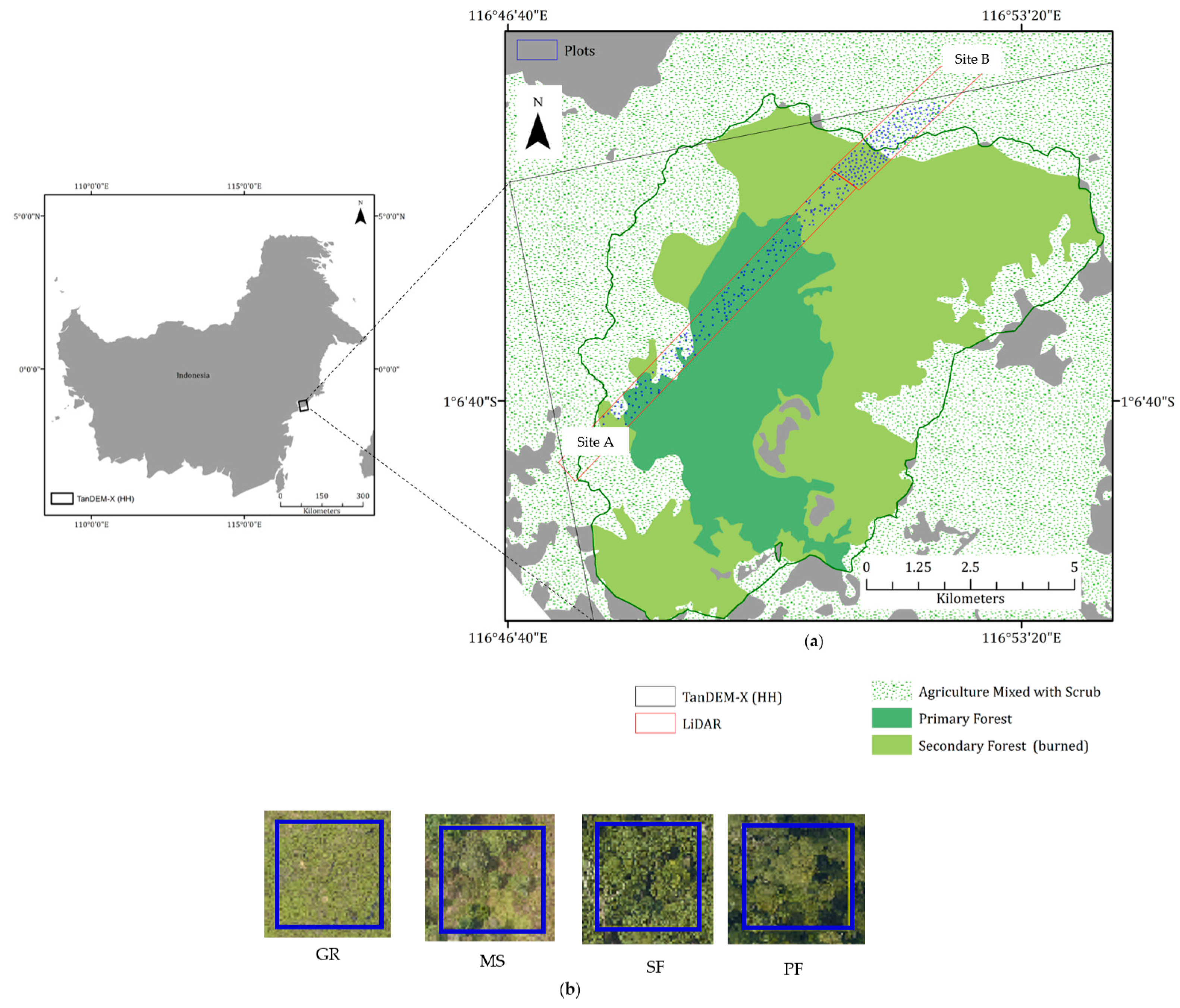
2. Study Site: Sungai Wain Protection Forest (SWPF), East Kalimantan (Indonesia)

Sungai Wain Protection Forest (SWPF) is located to the North of Balikpapan (116°46′14.08′′E, 0°59′57.91′′S), East Kalimantan (Indonesia) (Figure 1). The study site encompassed intact lowland Dipterocarp forest within the core of the SWPF surrounded by disturbed forest dominated by Macaranga sp. which developed after the 1997–1998 fires [62]. Cultivated areas are located to the North and to the East of the SWPF with mainly abandoned mixed rice fields, grassland which is dominated by the invasive Imperata cylindrica and scrub composed of a mix of vegetation at various stages of development. Intact lowland Dipterocarp forest in the SWPF reaches above-ground biomass up to 400 Mg/ha and heights up to 60 m [63] and on a large scale appears as homogeneous [62].

Elevation ranges between 30 and 140 m above sea level with an elevation gradient decreasing from North to South and terrain slope ranging from 0 to 30°. The soil type is classified as Alisols [41]. The climate is categorized as Tropical Wet [64], and is wet all year but has infrequent marked dry periods as a consequence of ENSO conditions. Its wet season, December to May, has peak rainfall in March (272 mm), with average annual precipitation equal to 2250 mm [65], and a rainfall minimum in July (147 mm during the dry season) [12]. The 1997–1998 ENSO, which affected the study area, was characterized by a lack of precipitation for several months, leading to fire which caused damage to two thirds of the SWPF [41]. As well as altering the species composition of the forest, there were noticeable changes in forest structure such as an increase in canopy openness [41].

3. Methods

3.1. TanDEM-X Data

TanDEM-X data was acquired on 11 December 2014 in StripMap bistatic mode (single polarization HH) at 41° incidence angle supplied through AO VEGE6702 by DLR (Figure 2). The scene covers 32 km W-E × 25 N-S km (UL Geo: 116°46′14.08′′E, 0°59′57.91′′S). A summary of the TanDEM-X acquisition configuration is found in

Table 1. TanDEM-X acquisition configuration parameters.

Parameter	Value
Mode	StripMap bistatic
Acquisition Date	11/12/2014
Polarization	HH
Incidence Angle (°)	41
Resolution (azimuth, range) (m)	3.3 × 1.8
Ground resolution (m) at 41°	3.3 × 2.74
Effective Baseline (m)	223
HoA (m)	30.2
Orbit direction	Ascending
Look direction	Right

. The data was processed using ENVI/SARScape 5.0 Interferometric module to generate coherence modulus and a Digital Surface Model (DSM) [67] and consists of the following steps: (a) interferogram generation (2 looks in azimuth and 2 looks in range); (b) retrieval of a subset of the SRTM-4 version DEM which covers the extent of the TanDEM-X acquisition; (c) interferogram flattening; (d) filtering using a Goldstein filter [68] and coherence generation; (e) phase unwrapping using the minimum cost flow algorithm; and (f) geocoding at 4.6 m resolution to WGS84 datum, Zone 50 South. A DSM was generated using the phase to height conversion by setting relaxed interpolation since the low coherence values meant that the phase was difficult to unwrap (Figure 2). The derived DSM was also geocoded at 4.6 m pixel spacing to WGS84 datum, UTM Zone 50 South. The DSM derived from TanDEM-X corresponds to the superimposition of the bare earth (Digital Terrain Model—DTM) plus the vegetation and corresponds to the phase center height (PCH) which is located within the vertical structure of the target [51]. The location of the PCH depends on target parameters (e.g., vegetation spatial configuration such as volume density) and the sensor’s parameters (e.g., frequency and polarization) [69].

3.2. Reference Datasets

LiDAR data was acquired on 14 November 2014 using the Optech ORION M300 system (frequency: 55 Hz). The airborne LiDAR instrument was flown at an altitude of 700 m above ground level, scan angle of ±18°, swath width of 455 m with an overlap of 227 m. The resulting point density was 5.75 points per m² (excluding overlap). The vertical accuracy for all LiDAR returns on clear ground was 0.08 m (standard error at 1 sigma). The data covers 9.7 × 0.7 km² (Site A) and 4.5 × 0.8 km² (Site B). The LiDAR products were geocoded to WGS84 datum, Zone 50 South. Lidar2dems open source software developed by Applied GeoSolutions was used to process the LiDAR data to provide the following: a Canopy Height Model (CHM) at 1 m resolution was generated by subtracting a Digital Terrain Model (DTM) from a Digital Surface Model (DSM) (Figure 2). The general term Digital Elevation Model (DEM) is used to refer to DSM, DTM or CHM.

A land cover map developed by the Indonesian Ministry of Forestry [66] was also used to distinguish between broad vegetation classes with additional visual inspection of aerial photography (Figure 1).

Aerial photos (AP) (0.5 m resolution) were acquired at the same time as the LiDAR overpass using a Trimble 80 megapixel medium format digital aerial camera. The APs were used as reference data to aid in the supervised analysis for the selection of classes of interest, since ground truth data was not available. The APs were deemed suitable to aid the selection of structural classes since they were able to capture illumination variability giving rise to textural differences derived from the spatial arrangement of canopy components (combination of sunlit or shadow areas), and so could be used to locate areas with different structural properties through visual inspection.

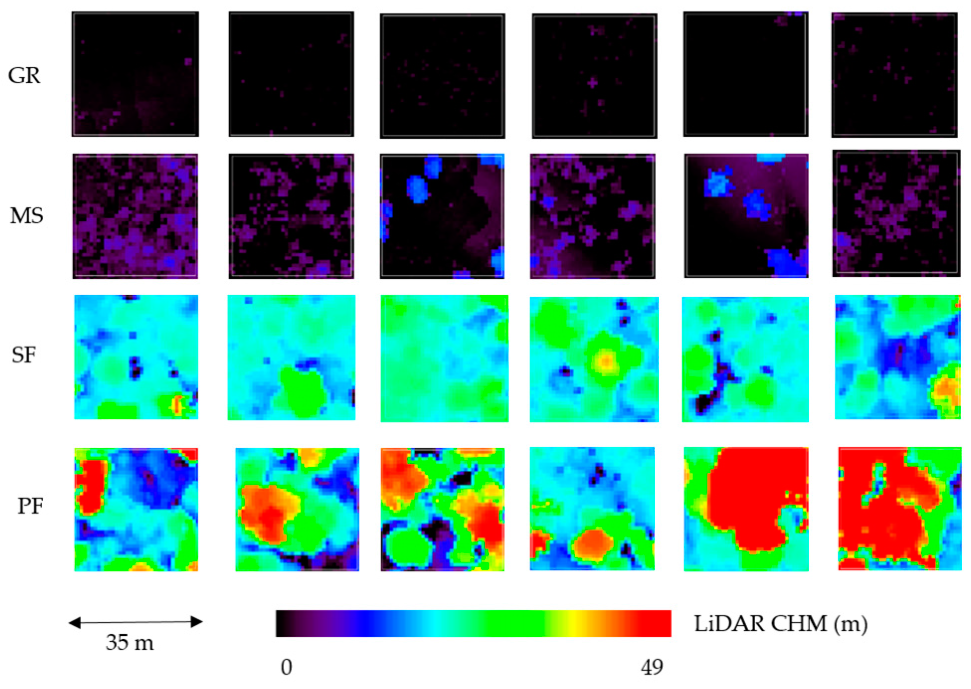
3.3. Vegetation Structural Class Selection

Analysis was performed in 315 virtual plots (35 × 35 m² = 0.12 ha) located in primary lowland Dipterocarpaceae forest (intact) (PF), secondary forest (disturbed) (SF), mixed scrub (MS) and grassland (GR). Figure 3 shows a representative sample of plots for each class visualized on a LiDAR CHM. A random sampling approach was devised within the extent of both the LiDAR and TanDEM-X datasets so that the number of non-overlapping plots of size 35 × 35 m² could be maximized without user interference. The choice of window size was determined from the knowledge of the landscape taking into account the spatial arrangement and size of canopies so that the variability was appropriately captured. It could not be smaller as the largest crown dimensions were in the range of 10–20 m in the intact primary forest (PF) and considering the random sampling approach ensured that the plots were not selected by the user so that the window was not centered on a single emergent crown, and if any larger plots might have contained a mixture of forest types, and the resolution of any eventual product using windows of this size would be reduced.

Class selection was based on a land cover map derived from Landsat developed by the Indonesian Ministry of Forestry [66] and on visual interpretation of high resolution aerial photography (0.5 m resolution). The class “mixed agriculture and scrub” described in the Indonesian Ministry of Forestry land cover map was broad and not representative of the condition in 2014 (as observed from aerial photography) thus, it was deemed appropriate to partition the class into two separate classes: grassland (GR) and mixed scrub (MS) based on visual inspection. The MS class is composed of a combination of Imperata cylindrica and presents taller re-growing vegetation such as shrubs and young trees which are not present in the grassland class (GR) which is prevalently colonized by Imperata cylindrica.

Landscape heterogeneity from 2D wavelet spectra was assessed based on randomly selected pixels which are representative of the chosen classes (PF, SF, MS and GR) to give insight into the target structure at four scales of decomposition based on a LiDAR CHM and TanDEM-X DSM (the figure in Section 4.2). The set of cases considered are as follows: (a) Emergent trees in a multi-layered heterogeneous (in terms of heights) matrix characteristic of old-growth forest (PF); (b) Relatively homogenous secondary forest patches composed by a carpet of crowns with high clumpiness. Absence of tall emergent trees but has reached full canopy cover (SF); (c) Early stage re-growth presenting smaller tree crowns (2–3 m) closely packed but discernible from LiDAR (MS); (d) Homogeneous grassland (Imperata cylindrica) presenting low height with scattered small shrubs (GR).

3.4. LiDAR and TanDEM-X Texture Correlation Analysis to Assess Impact of Topographic and Canopy Structures

Scaling (spectral) analysis of LiDAR and TanDEM-X datasets was performed in the wavelet domain along a profile covering 6.95 km in a north-south direction dominated by PF and SF. The aim of the analysis was to identify scales where textural patterns associated with topographic or canopy features develop within the different Digital Elevation Models (DEMs). The following two-point spatial statistics were computed in the wavelet domain [70]: (a) wavelet variance; and (b) wavelet co-variance (between LiDAR DTM/DSM, LiDAR DTM/CHM, and LiDAR DTM/TDX DSM). A wavelet representation is used instead of a Fourier one because the processes are multi-scale and non-stationary. The analysis provided an assessment of the relative influence on the signal texture of topographic structures and canopy structures, which is the main concern of the current study.

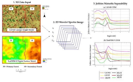
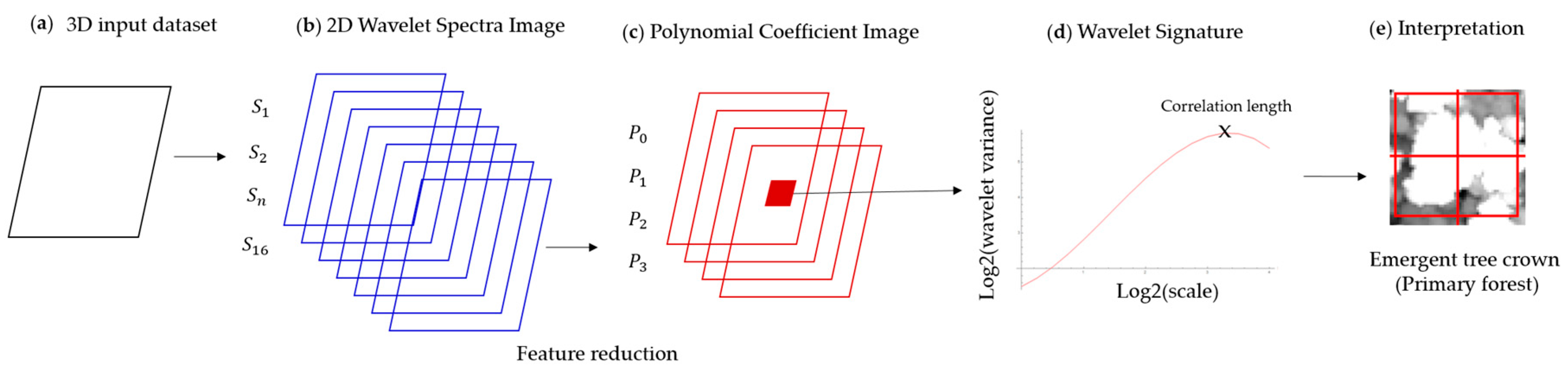
3.5. 2D Wavelet Spectra

Information on canopy structure is carried by datasets where vegetation height (or a proxy) is mapped as a function of space (e.g., LiDAR CHM or TanDEM-X DSM) (Figure 4). This mapping provides a two-dimensional random field, whose spatial (two-point) statistics condenses measures of the horizontal and vertical distribution of the forest. These random fields are analyzed using two-point statistics provided by the variance of a wavelet frame that acts as a differential operator (Equation (1)). This statistics, analogous to the structure function lends to the characterization of stationary random processes, as well as of non-stationary processes with stationary increments (e.g., fractals) [29].

$$\langle WS{(s, x)}^2\rangle \cong \langle (f(x+s)-f{(x)}^2)\rangle$$

(1)

In particular, we consider exploiting the well-known properties of optimal space-frequency resolution of wavelets, and local (in space) estimates of the wavelet variance as a function of scale.

At each point in space (at each pixel location of the analyzed image), we obtain, in the log–log variance/scale place, a characteristic signature of the process, which reflects process parameters, such as field roughness, correlation structures and intermittency. This data structure is called “2D wavelet spectrum” ($\mathrm{WS}$), and it is an extension of the method developed by De Grandi et al. [70]. In more detail, the input field (e.g., vegetation height image) is decomposed in the wavelet frame basis using four dyadic scales. Local estimates of the wavelet variance are obtained by convolving the square of the wavelet coefficients with a B-spline smoothing function (Equation (2)).

$$WS\left(s, i, j\right) = \left(c_{x,s}{\left(i, j\right)}^2+c_{y,s}{\left(i, j\right)}^2\right)\otimes {\beta }_{i,j}$$

(2)

Each signature ${\log }_2\mathrm{WS}$ (${\mathrm{LiDAR}}_{\mathrm{CHM}}\mathrm{WS}$ or ${\mathrm{TDX}}_{\mathrm{DSM}}\mathrm{WS})$ is interpolated in scale with a step of ¼ and fitted by a 3rd degree polynomial function. This function provides a good approximation to the wavelet signatures [70]. Four polynomial coefficients for each pixel of the input field constitute finally the dimensionally reduced features that describe the 2D wavelet spectrum. Two-point statistics was generated by deriving four polynomial coefficients: for LiDAR CHM (${\mathrm{LiDARCHM}}_{{\mathrm{P}}_0}$, ${\mathrm{LiDARCHM}}_{{\mathrm{P}}_1}$, ${\mathrm{LiDARCHM}}_{{\mathrm{P}}_2}$ and ${\mathrm{LiDARCHM}}_{{\mathrm{P}}_3}$ and for TanDEM-X DSM (${\mathrm{TDXDSM}}_{{\mathrm{P}}_0}$, ${\mathrm{TDXDSM}}_{{\mathrm{P}}_1}$, ${\mathrm{TDXDSM}}_{{\mathrm{P}}_2}$ and ${\mathrm{TDXDSM}}_{{\mathrm{P}}_3}$). Pixel based analysis was undertaken to explore the sensitivity of 2D wavelet spectra to canopy structure heterogeneity through a gradient of varying vegetation structure (PF, SF, MS and GR) (see Section 3.3).

3.6. Separability

To assess statistically the separability between four classes afforded by the wavelet spectra polynomial representation the Jeffries–Matusita (JM) distance was computed. The JM distance of a pair of probabilistic distributions indicates the average distance between two classes density functions and it features a saturating behavior with increasing separation [71]. This fact makes it more suitable for dealing with a multi-class problem, because it avoids bias when taking averages due to an easily separable class. It is therefore suitable for the problem at hand, which has four features and four classes. The JM distance (Equation (3)) is derived from the Bhattacharyya distance (BD) (Equation (4)) [71]. The JM distance ranges between 0 and $\sqrt{2}$ with highest values indicating greater class separability [71].

$$J{M}_{ij} = \sqrt{2(1-e^{-BD})}$$

(3)

where BD:

$$BD = \frac{1}{8}{\left(M_i-M_j\right)}^T\left[\frac{C_i+{C_j}^{-1}}{2}\right]\left(M_i-M_j\right)+\frac{1}{2}ln\left[\frac{\left|\frac{C_i+C_j}{2}\right|}{\sqrt{\left|C_i\right|\left|C_j\right|}}\right]$$

(4)

where $i$ is the class with mean vector $M_i$ and co-variance matrix $C_i$.

Pairwise JM resulted in six JM distances, which are averaged and normalized by dividing the theoretical maximum JM distance of $\sqrt{2}$. The normalised average JM distance was used as a parameter to indicate overall class separability [71]. Upper and lower bounds of the probability of the classification error $P_e(i,j)$ are given by [71] (Equation (5)):

$$\frac{1}{16}{(2-J{M}_{i,j}^2)}^2 \le P_E\left(i,j\right) \le 1-\frac{1}{2}(1+\frac{1}{2}J{M}_{i,j}^2)$$

(5)

The JM distances are computed for the six combination of class pairs among GR, MS, SF, PF, and feature vectors $\overrightarrow{v_{x,y}} = \left\{P_0,P_1, P_2, P_3\right\}$, where $P_i$ are the polynomial coefficients of the wavelet spectra averaged over the training set plots, defined as described in Section 3.3. Moreover, to investigate the dependence of class separability on scale, the JM distance is also computed for each scale of the signature separately $\langle W^2\rangle = f(scale)$ derived from the polynomial coefficients. In this case, the feature space is one-dimensional.

4. Results and Interpretation

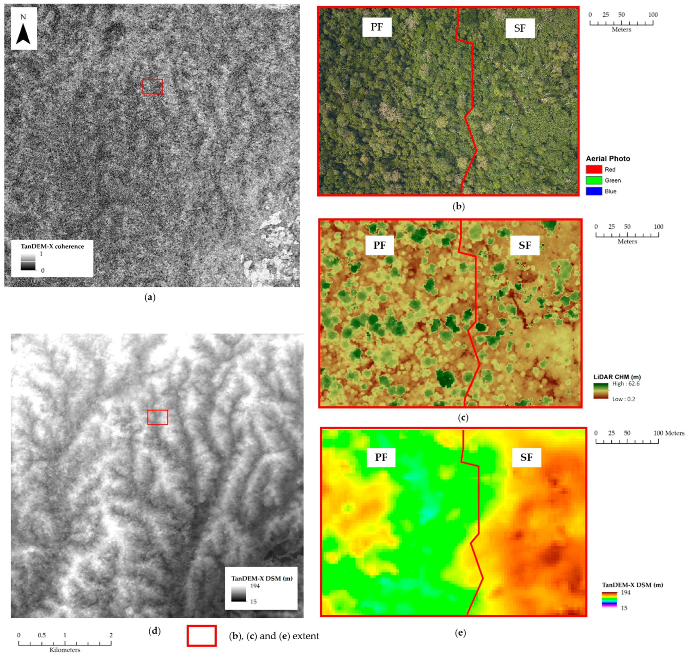
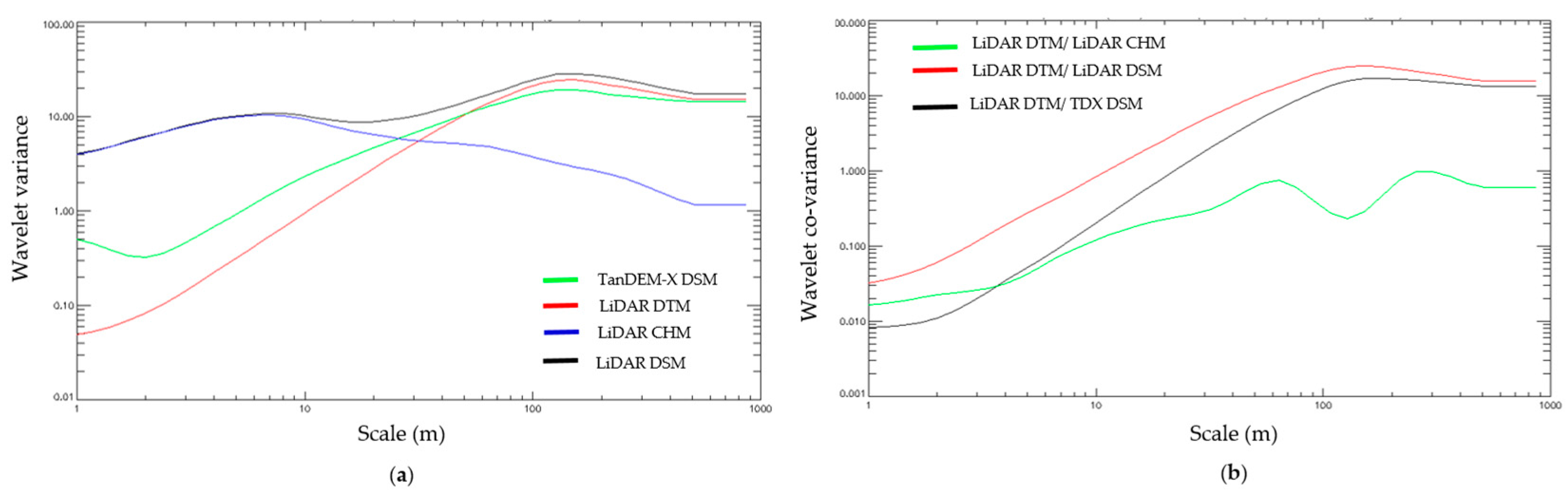
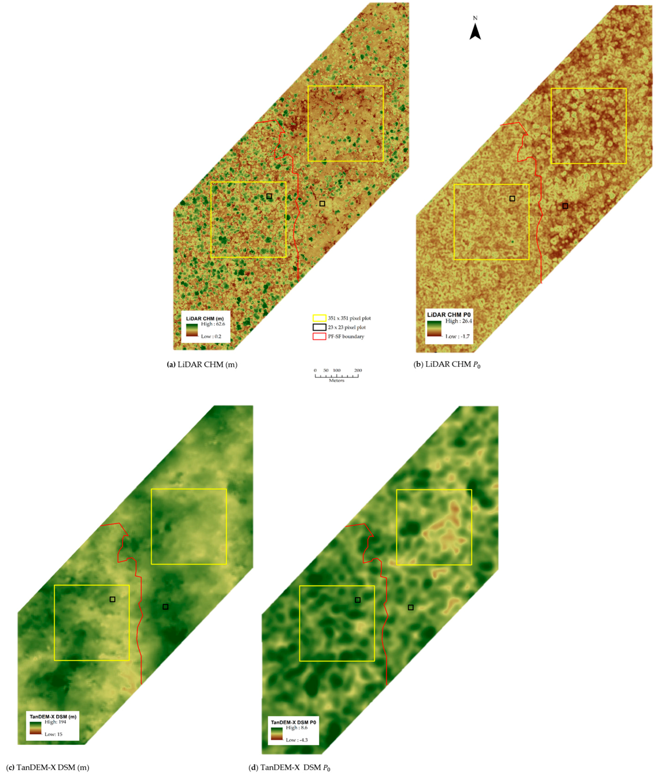
4.1. LiDAR and TanDEM-X Textural Correlation Anaysis to Assess Coupling of Topographic and Canopy Structures

Canopy structure (roughness) measures derived from 3D datasets can provide information on landscape disturbance and recovery [25] but can be affected by environmental factors [53] such as the underlying topography especially in steep terrain [54]. Since the transect is characterized by low-lying undulating terrain (52.7 ± 3.2 m) and often the presence of mild slopes (12.1° ± 10°) and at higher elevation (81.4 ± 11.2 m) and slopes (12° ± 4.3°) in AG and MS plots (elevation: 64.9 ± 21.4 m, slopes: 11.9° ± 6.2°), understanding of topographic structure is important to gain a better insight on the processes that play a role and the extent to which they influence the 3D information provided by LiDAR and InSAR. This is especially relevant as only the LiDAR provides both a DSM and DTM, and thus the possibility to calculate a CHM; TanDEM-X only provides a DSM.

The wavelet variance, being a two-point statistic proxy of the structure function, bears information on the dominant correlation patterns associated with either topographic or canopy structures, these happening at different scales and can also give insight into the impact of topography and canopy structure by comparison with the available LiDAR DTM which carries information on ground topography (Figure 5a). To test this we performed an analysis over the 6.95 km transect in primary and disturbed forest, considering the LiDAR and TanDEM-X data. The LiDAR DTM (red) signature reveals the trend of a process with smooth texture at short scales and long memory (correlated patterns) up to 200 m. This scale corresponds to the onset of regular (almost periodic) patterns induced by the topography from the hilly terrain, which is reflected on the LiDAR DSM (black) and the TanDEM-X DSM (green), while the LiDAR DSM (black) carries strong information of short scale texture, with correlation length of tens of meters. Importantly, this texture patterns is also present (exactly overlaid) in the LiDAR CHM (blue) signature, revealing that within the short scale range (between 1 and 10 m) the textural information is related to canopy structure and not to topography. The TanDEM-X DSM (green) is also sensitive to these short scales structures due to canopy variation (i.e., variance greater than LiDAR DTM) but with lower separation with respect to variance due to topography (LiDAR DTM).

The wavelet co-variance holds information on the textural correlation between datasets, these being the LIDAR DTM, DSM and CHM and the TanDEM-X DSM (Figure 5b). The LiDAR DTM-DSM (red) confirms the presence of structures (periodic patterns) in the DTM texture at correlation length of 200 m (scale 2⁸), which are reflected onto the DSM texture. At shorter scales, the texture correlation between LiDAR DTM and TanDEM-X DSM (black) is one order of magnitude lower, especially at scales typical of canopy width and gaps. This fact reinforces the point that although the TanDEM-X DSM is affected by the DTM noise, information on vegetation structure can still be detected as it happens at a different scale range. However, there is a striking feature in the LiDAR DTM/CHM co-variance (green) that reveals that there is also a textural reflection of topographic structures onto the LiDAR CHM, although at two orders of magnitude less important. Still, even if it is a weak coupling, this could mean that the LiDAR CHM has a component that follows the strong topographic features at scale of 200 m. This coupling could confirm the fact that forest in valleys is higher than forest on ridges. This is due to several factors such as: (1) higher soil fertility and moisture availability in valleys; and (2) more need for forest in valleys to grow taller to reach light (light competition) [38].

The results is key to determine the potential of TanDEM-X DSM for detecting canopy heterogeneity over larger areas compared to airborne LiDAR since TanDEM-X provides global coverage [57]. Moreover, as opposed to a CHM the characterization of canopy heterogeneity does not depend on the availability of ground topography (DTM) but relies on the canopy roughness information provided from a DSM which does not penetrate deep enough into the canopy to reach the ground (in the presence of dense tropical forest) and therefore is restricted to a layer located somewhere within the upper canopy [72]. Limitations due to resolution are to be taken into account since this is lower for TanDEM-X and it does not enable to resolve single crowns as in the high resolution airborne LiDAR. The results have implications on the utility of LiDAR CHM but most importantly the potential of TanDEM-X DSM, which can provide complementary information on canopy roughness.

Further analysis was undertaken at short scales (between scale 2⁰ and 2⁴). Longer scales were not considered since the ground topography was found to play an increasingly important role in affecting the process. Future research which aims to link textural variations to forest parameters (e.g., crown dimensions, height and above-ground biomass) should take into account the influence of topography to avoid bias in the estimation of these parameters which could be caused by the underlying relief rather than structural parameters [73].

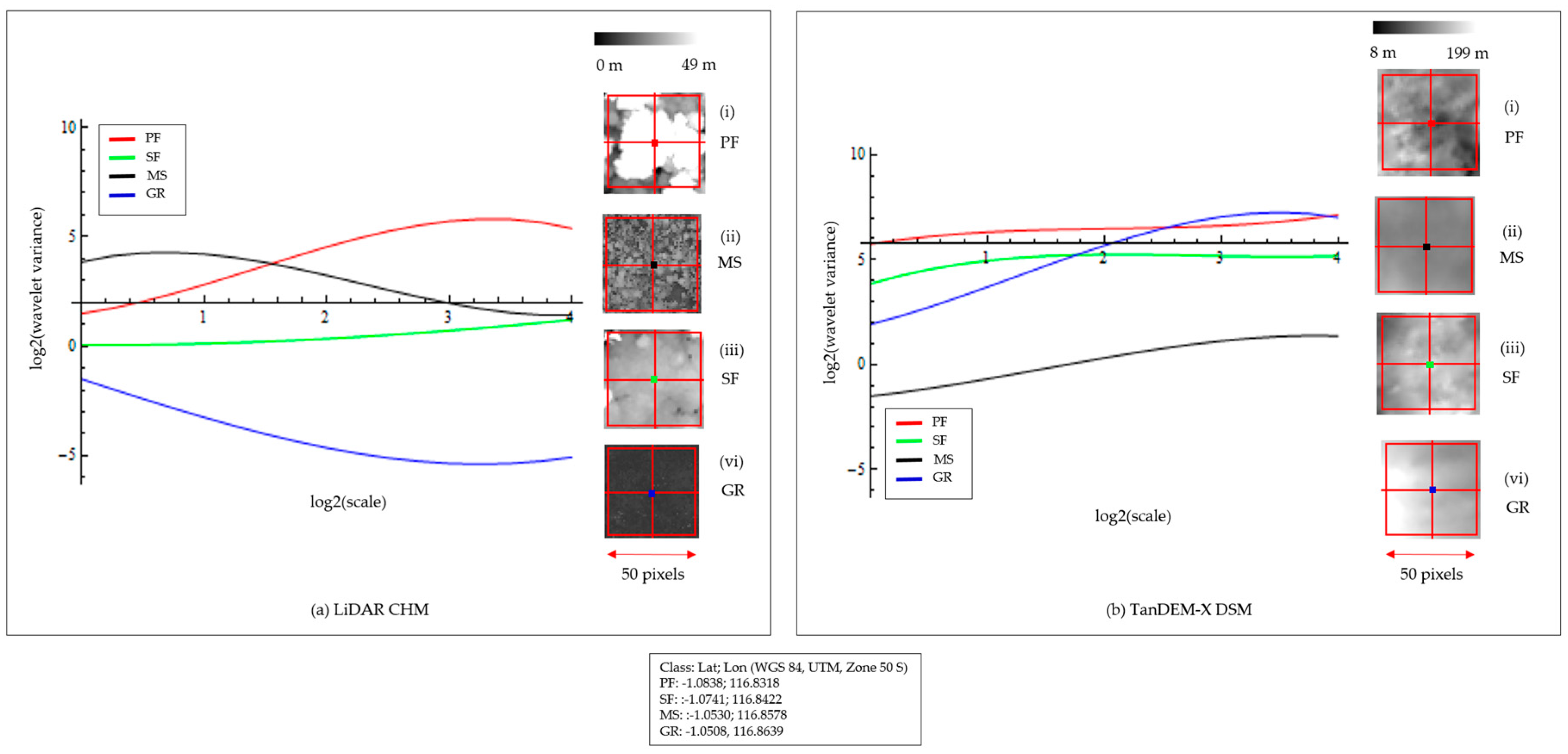
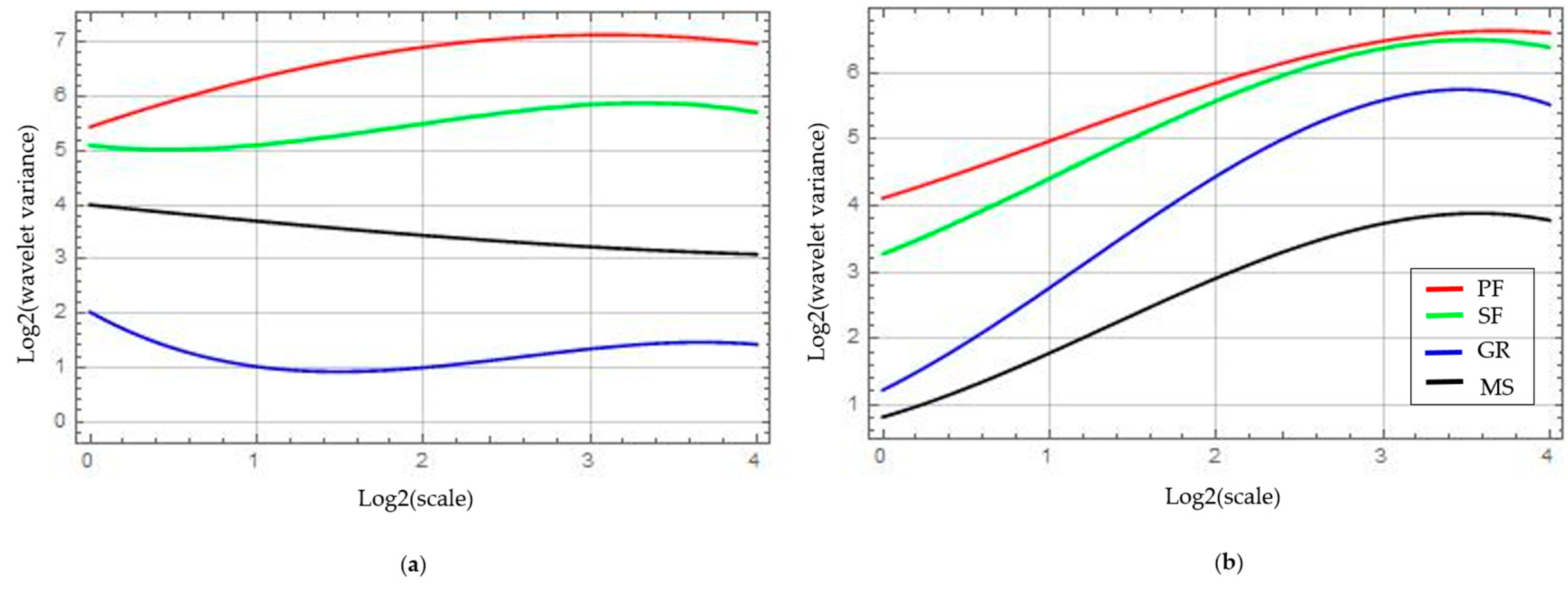
4.2. Canopy Structural Heterogeneity Based on 2D Wavelet Spectra

Airborne LiDAR CHM is optimal to gain understanding of the processes driving the wavelet signature due to the high resolution (1 m) and thus, the ability to resolve single crowns. Individual spectrum data points, one in each of the four land cover types (each corresponding to the local wavelet variance as a function of scale, i.e., a wavelet signature) were considered in order to help in the interpretation of wavelet spectra of a LiDAR CHM. Each spectrum sample corresponds to a local wavelet variance estimate at one point in space and for all scales (i.e., a wavelet signature). The interpretation of the wavelet signatures is based on two main considerations: (a) extent to which the process presents self-similarity (correlation length); and (b) wavelet variance absolute values for a set of landscape heterogeneity cases is illustrated in Figure 6.

Wavelet signatures for a multi-layered, complex old-growth forest patch (PF) (red line) dominated by a large emergent crown (18 m) show the typical trend of stationary noise with an exponential autocorrelation function (increasing variance with scale, asymptotically converging to the process variance). Wavelet variance for PF ranges between 1.5 and 5.4 with a maxima (correlation length) around scale 2³ (8 m). Of course, this figure must not be interpreted as a crown width measure, but as the neighborhood within the crown where the canopy height variations are still correlated. This can be verified by interpretation of inset (Figure 6a(i)) showing the presence of a large emergent crown surrounded by coalescing large crowns.

The flat wavelet signature for a pixel selected in SF (Figure 6a(iii)) composed of interlocking crowns of similar height (homogeneous structure) with a lack of emergent trees is markedly different from that of the heterogeneous PF. The signature is typical of a white noise process meaning that the process is scale invariant and also presents no correlation length meaning that the process is self-similar at all scales considered and this is due to the homogeneity of the forest patch, it does not present correlated features. The wavelet variance (in this case proportional to the scale variance) is lower compared to that of PF (range between 0.06 and 1.2).

The MS class signature (black line) reveals the presence of non-stationarity with full multi-scale correlation patterns (decreasing variance with increasing scale), and a first correlation length at short scale (2 m). This is because the size of crowns located in MS (as seen in Figure 6a(ii)) is much lower (1–2 m) compared to the size of emergent tree crowns in PF (Figure 6a(i)).

The GR class wavelet signature also presents a white noise process, with the lowest process variance. The corresponding LiDAR CHM pixel selected is shown in (Figure 6a(vi)) and is clearly dominated by a layer that is texturally homogeneous and featureless.

The corresponding TanDEM-X DSM analysis does not match with the LiDAR CHM analysis. This highlights the fact that the sensor resolution is of key importance in textural measures. The two forest classes (PF and SF) (red and green line) behave in a similar way, with the signatures revealing white noise processes. This is due to the fact that now single canopies cannot be resolved, and the correlated patterns appearing at 1 m resolution in the LiDAR CHM signatures are now not visible.

Nonetheless, the PF process features a higher process variance (Figure 6b(i)), meaning that still some discrimination between PF and SF is possible with the one-point statistic. The MS signature (Figure 6b(ii)) is again white noise and presents the lowest process variance. Again, this is due to the fact that smaller crowns cannot be resolved. Importantly, the GR signature (Figure 6b(vi)) reveals a stationary correlated process, with a still around 8 m (scale 2³). This is ascribed to the influence of topography. Indeed, as these areas are dominated by surface scattering, from the spatial statistic (texture) point of view, the main dependence comes from the terrain height variations, whereas, in forested areas, volume scattering moves the PCH upwards towards the canopy upper layer and limits penetration capabilities.

4.3. Interpretation of Wavelet Measures of Structural Heterogeneity Based on Height Variance

4.3.1. Wavelet Signatures Polynomial Fit

Probability distributions (PD) for the first wavelet polynomial coefficient ($P_0$) derived from the 3rd order fitted polynomial are found in Figure 7. $P_0$ is the intercept with the y-axis in the log–log variance–scale plot, therefore it is a good approximation to the variance at short scale. From Section 4.1 we assume that most of the variation due to canopy structures occurs at short scale and thus, $P_0$ holds more information compared to the other polynomial coefficients ($P_1$, $P_2$ and $P_3$).

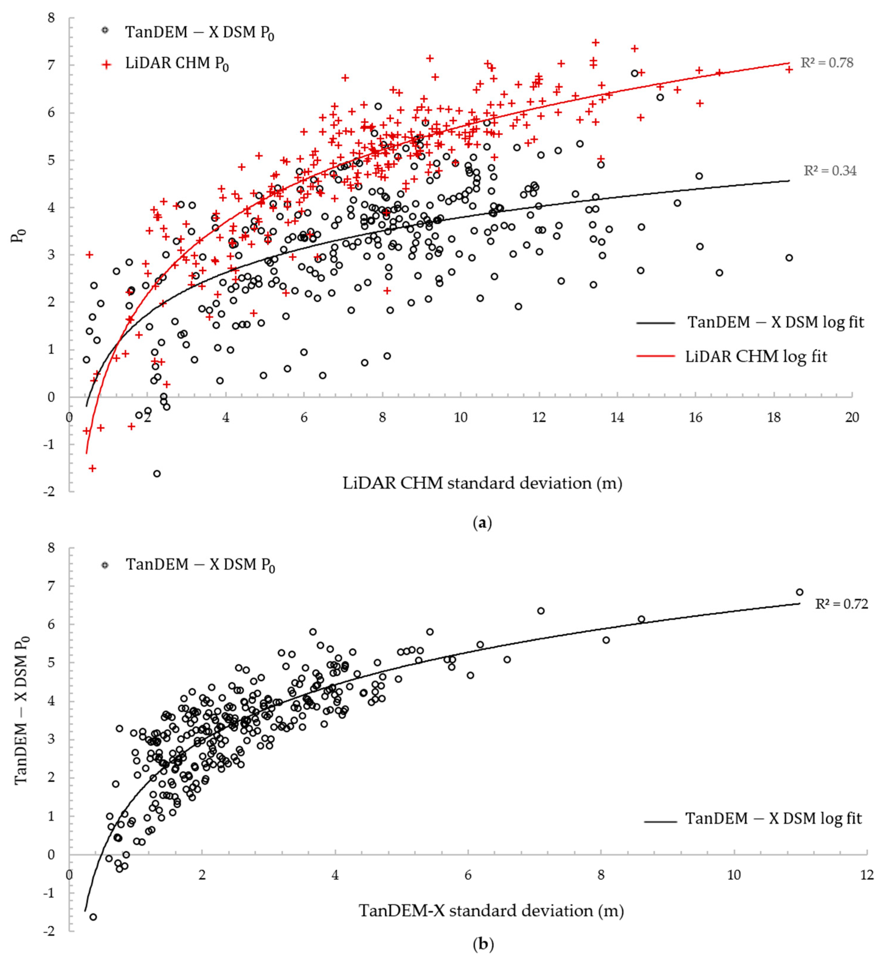
4.3.2. Regression Analysis

In order to gain insight into the measures provided by the wavelet spectra and their mapping onto the physical characteristics of the observed random field (forest structural heterogeneity), a regression analysis was performed between the LiDAR CHM standard deviation and the LiDAR CHM $P_0$. $P_0$ is the constant term of the wavelet variance polynomial approximation. Therefore, it provides a figure of the overall variance (energy) carried by the wavelet representation. $P_0$ is also the intercept with the y-axis in the log–log variance–scale plot, therefore it is a good approximation to the variance at short scale.

We found that the LIDAR CHM $P_0$ is well correlated with the standard deviation of the LiDAR CHM (R² = 0.77, N = 315) (Figure 8a) and the TanDEM-X DSM $P_0$ is also well correlated with the standard deviation of the TanDEM-X DSM (R² = 0.72, N = 315) (Figure 8b). This means that the two-point statistic ($P_0$) at short scale of the process carries the same information as the one-point statistic (standard deviation) of the same process. Moreover, the one-point statistic of the TanDEM-X DSM is also equivalent to the CHM two-point statistic. This point confirms that, at least at first order, the properties of the CHM process are reflected onto the TanDEM-X DSM process.

On the other hand, the LiDAR CHM standard deviation was weakly correlated with TanDEM-X $P_0$ (R² = 0.34, N = 315). This case indicates that the TanDEM-X DSM process is not related in a simple way to the CHM process, but it is the result of the superposition of several random processes, such as terrain topography and InSAR phase signal to noise ratio. Therefore, the textural dependency of the DSM cannot be measured only by a simple one-point statistic, or a one-scale two point statistic, but the full multi-scale measures (wavelet spectra) must be called into play.

Finally, notice that the correlation between the two-point statistic $P_0$ and the one-point statistic (standard deviation) of the same process (Figure 8a) is in line with the claim that the wavelet variance is an asymptotic unbiased estimator of the process variance [74]. Indeed, given the wavelet frame of choice that acts a differential operator, the wavelet variance is tantamount to (Equation (6)):

$$\langle W{(x, \tau )}^2\rangle = \langle {(f\left(x\right)-f(x+\tau ))}^2\rangle \tau \to \infty \stackrel{yields}{\to }2(\langle f^2\rangle -{\langle f\rangle }^2) = 2VAR(f)$$

(6)

Often in old-growth tropical forest height differences between individual trees is significant as a result of the presence of emergent trees [75]. The results are in line with findings based on optical sensors that indicate that texture is driven by the variation in vertical structure (presence of emergent trees) of the canopy and gives rise to canopy texture [76]. Stands with a high variance in tree height have a rougher upper canopy compared to those with lower variance [76]. However, in DEMs provided by ranging or interferometric sensors (e.g., from LiDAR or InSAR), texture is not related to shadowing effects but to the gradient of height information. The area covered by large emergent trees (>35 m) in SF (burned) plots is significantly different from PF (p < 0.01, N = 222). This is a good indicator to explain why SF presents a lower canopy roughness compared to PF.

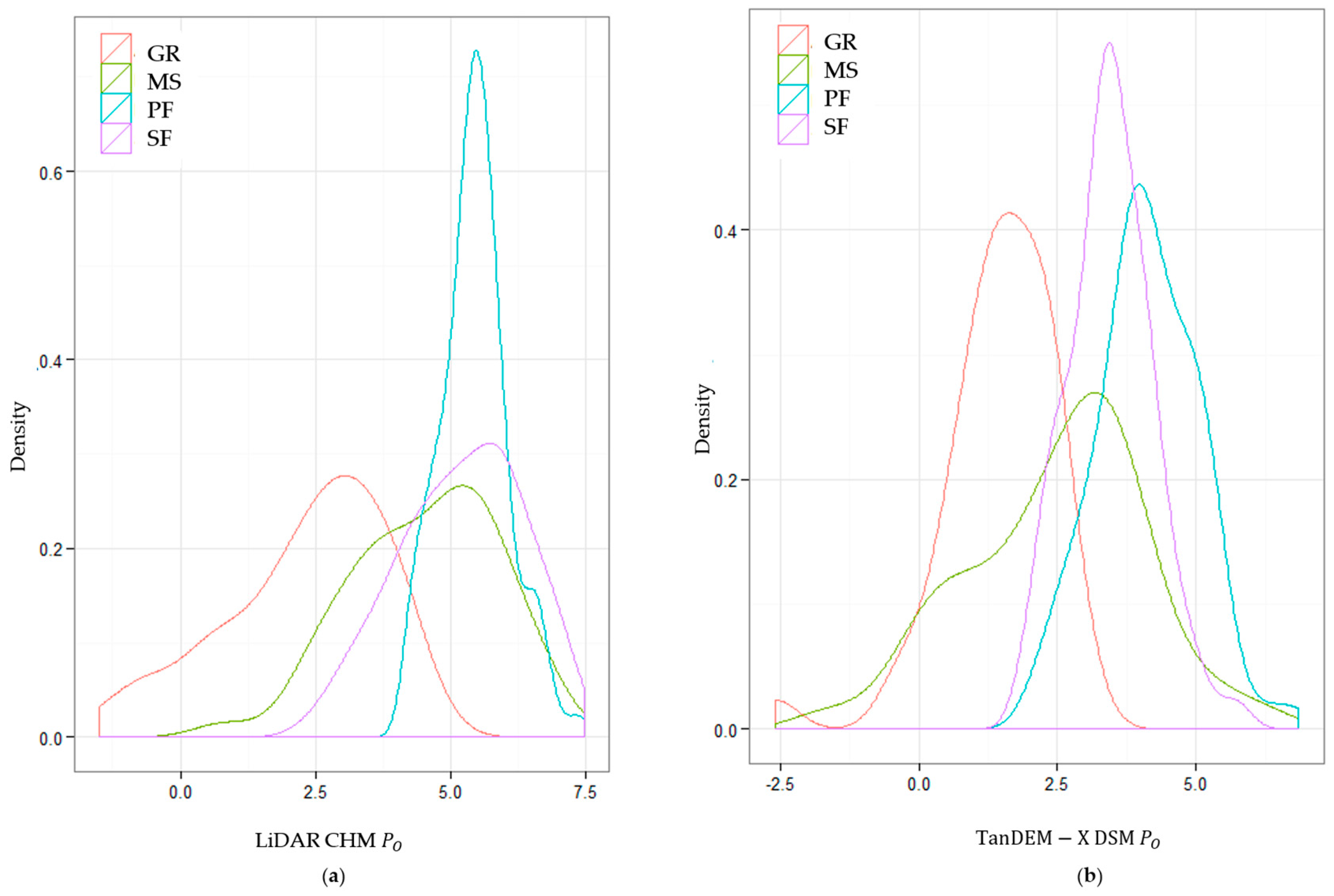
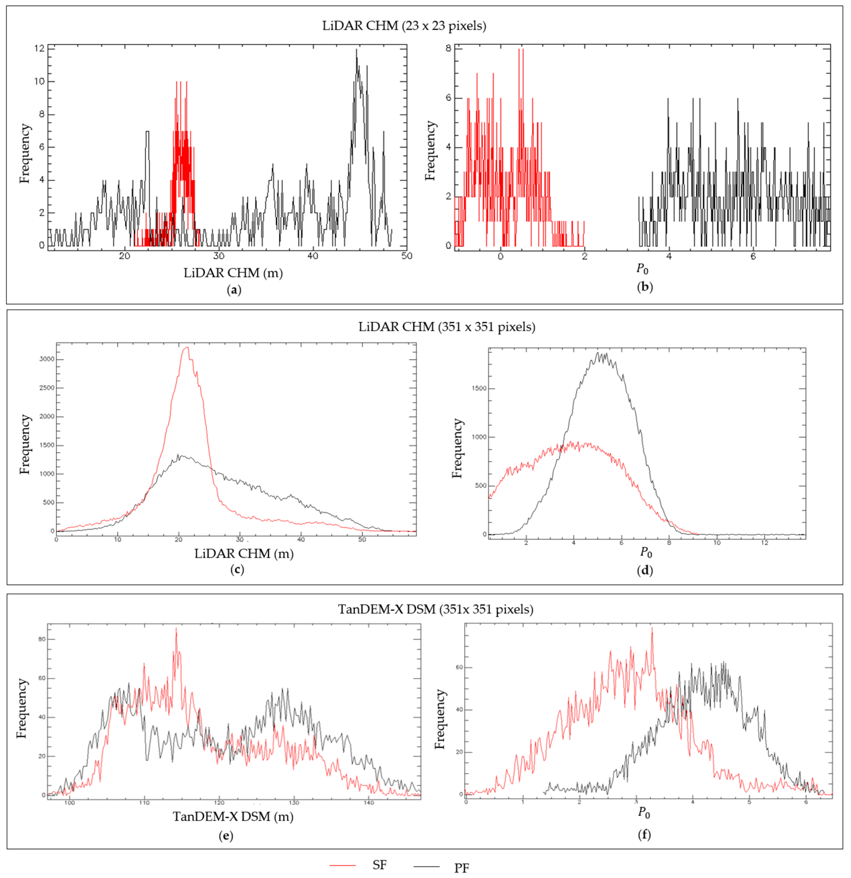
4.3.3. LiDAR CHM and TanDEM-X Polynomial Coefficients and Standard Deviation Frequency Distributions

LiDAR CHM (height) frequency distribution (FD) in a 23 × 23 pixels (0.05 ha) area presenting low LiDAR CHM $P_0$ (0.12 ± 0.65) (mean± standard deviation) (SF) was compared with an area presenting high $P_0$ (5.6 ± 1.2) (PF) (Figure 9b). Indeed, the area with lowest $P_0$ (SF) presents a more homogeneous height distribution, ranging between 21.1 and 27.9 m (mean ± standard deviation) (25.9 ± 1.1) (Figure 9). Conversely, higher $P_0$ (black line) (Figure 9b) corresponds to a more heterogeneous structure comprising tree heights ranging between 11.8 m and 48.3 m (34.6 m ± 10.7 m) (Figure 9a).

Lower tree height standard deviation (in this case provided by LiDAR CHM) observed in SF is often associated with young even aged stands of mono-dominant species [76]. Another independent dataset such as field data would be required to confirm this assumption. The forest successional gradient ranging from intact to burnt and ultimately regrowth and the variance of the CHM has been observed in other studies based on optical remote sensing, whereby the presence of emergent crowns caused a significant shadowing effect on the lower vegetation in PF influencing texture from spectral information [76].

Analysis taking into account 351 × 351 pixels plots of PF and SF was explored (Figure 9c–f). At this scale the LiDAR CHM FD indicates that the SF heights are no more restricted to the 21–27 m range like in the sub-hectare case (Figure 9a). However, there is a clear predominance around 22 m in the SF (Figure 9c). The SF also presents a long tail (not present in the sub-hectare case), which corresponds to patches that have not been burned within the burned matrix. Instead, homogeneous patches are areas where forest was affected by fire, and, after 17 years, a forest successional stage with a more uniform structure replaced heterogeneous old-growth formations. Because of the complex composition unburned small forest islands patches surrounded by burned forest, they will be more prone to fire disturbance since future fires will be facilitated by the more open canopy [15]. Instead the PF presents a distribution ranging from 0 to 59 m (mean ± standard deviation: 27 ± 9.5 m) (Figure 9c). At hectare scales the PF is still very heterogeneous and multi-layered, a characteristics observed in many tropical forests studies due to the high diversity of species [24].

Similar, effects can be noticed in the TanDEM-X DSM (Figure 9f) where SF $P_0$ ranges between −0.02 and 6.5 (mean ± standard deviation: 2.9 ± 1.0), while PF $P_0$ ranges between 1.3 and 6.3 (mean ± standard deviation: 4.2 ± 0.8). In this case, the one-point statistical separation between PF and SF is less evident due to two reasons: coarser resolution (4.6 m); approximation of the top canopy spatial variation provided by location of the coherence PCH, this in turn depending on the canopy volume density and the sensor’s parameters [69]. However, notice that the distribution based on TanDEM-X DSM $P_0$ still bears information related to structural differences between PF and SF.

We can conclude that textural variation between SF and PF, as measured by one-point statistic (LiDAR CHM height FD) depends on the scale of observation and the disturbance conditions (e.g., presence of unburned forest patches within a burned forest matrix). This process has been observed in other tropical forest settings where, unburned forest patches were still present within the burned forest [77,78]. In this particular case, they formed connected ribbons of old-growth forest along streams [38] and they were not burned since the flammability in the presence of higher moisture is lower compared to those areas further away from water sources [15].

LiDAR CHM wavelet spectrum image ($P_0$) (Figure 10b) visual interpretation confirms the results from the FDs. Figure 10a shows a false color image of the LiDAR CHM, where the red line marks the boundary between PF and SF to illustrate how forest height varies across the LiDAR extent. Figure 10b shows the corresponding LiDAR CHM $P_0$. Lower LiDAR CHM $P_0$ (light green) indicates more homogeneous, even height forest patches while, high $P_0$ is represented in brown. The onset of the more homogeneous forest patches is clearly dominant in the region designated as the burned SF area of the SWPF to the North of the red line boundary. The TanDEM-X DSM (m) is shown in (Figure 10c) and the corresponding $P_0$ is illustrated in (Figure 10d) with low values in brown and high values in dark green. The results are further confirmed by class separability in the feature space of the wavelet spectra descriptors (Section 4.4).

4.4. LiDAR CHM and TanDEM-X DSM 2D Wavelet Spectra Class Separability

JM distance was performed based on the maximum number of common samples for each class pairs (GR/MS: 44, GR/SF: 44, GR/PF: 44, MS/SF: 49, MS/PF: 49, and SF/PF: 96).

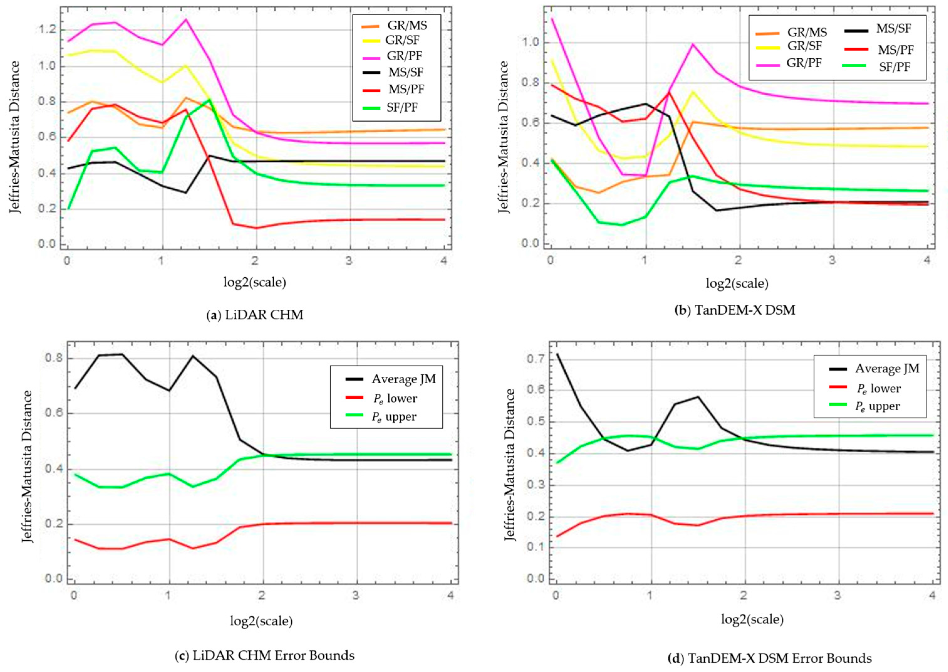
4.4.1. Scale by Scale Class Separability

${\mathrm{LiDAR}}_{\mathrm{CHM}}$ Wavelet Signature (${\mathrm{LiDAR}}_{\mathrm{CHM}}$WS) separability (see Section 3.5 for WS definition) at different scales was performed on pairwise JM to assess the scale at which class separability was greater (Figure 11a). The JM distance ranges between 0 and $\sqrt{2}$ with highest values indicating greater class separability. Best separability between GR/MS (${\mathrm{JM}}_{\mathrm{GR}/\mathrm{MS}}$ = 0.82), GR/SF (${\mathrm{JM}}_{\mathrm{GR}/\mathrm{SF}}$ = 1.0) and GR/PF (${\mathrm{JM}}_{\mathrm{GR}/\mathrm{PF}}$ = 1.26) was achieved at 2.4 m (scale 2^1.25), while the best separability between class pairs MS/SF (${\mathrm{JM}}_{\mathrm{MS}/\mathrm{SF}}$ = 0.49) and SF/PF (${\mathrm{JM}}_{\mathrm{SF}/\mathrm{PF}}$ = 0.81) was achieved at 2.8 m (scale 2^1.5). Best separability between MS/PF occurred at 1.4 m (scale 2^0.5) (${\mathrm{JM}}_{\mathrm{MS}/\mathrm{PF}}$ = 0.78).

Separability results considering ${\mathrm{TDX}}_{\mathrm{DSM}}\mathrm{WS}$ scale by scale (Figure 11b) indicate that the highest separability between class pairs is achieved at 4.6 m (scale 2⁰) for class pairs GR/SF (${\mathrm{JM}}_{\mathrm{GR}/\mathrm{SF}}$ = 0.91), GR/PF (${\mathrm{JM}}_{\mathrm{GR}/\mathrm{PF}}$ = 1.1), MS/PF (${\mathrm{JM}}_{\mathrm{MS}/\mathrm{PF}}$ = 0.80) and SF/PF (${\mathrm{JM}}_{\mathrm{SF}/\mathrm{PF}}$ = 0.41), while the highest separability between class pairs GR/MS (${\mathrm{JM}}_{\mathrm{GR}/\mathrm{MS}}$ = 0.61) is achieved at 13 m (scale 2^1.5) and at 9.2 m (scale 2¹) for class pair MS/SF (${\mathrm{JM}}_{\mathrm{MS}/\mathrm{SF}}$ = 0.70).

${\mathrm{LiDAR}}_{\mathrm{CHM}}\mathrm{WS}$ outperforms the ${\mathrm{TDX}}_{\mathrm{DSM}}\mathrm{WS}$ due to its higher resolution. Nonetheless, textural information derived from the ${\mathrm{TDX}}_{\mathrm{DSM}}\mathrm{WS}$ can still provide a certain degree of separability. Results also confirm that information at higher scales does not bear significant information on class separability and even the first few scales contain limited information when taken singularly. Analysis of the full $\mathrm{WS}$ is therefore essential to achieve improved separability.

4.4.2. Full Wavelet Signature (WS) Class Separability

Class separability results based on the full ${\mathrm{LiDAR}}_{\mathrm{CHM}}\mathrm{WS}$ and ${\mathrm{TDX}}_{\mathrm{DSM}}\mathrm{WS}$ using the JM distance are found in

Table 2. JM distance separability between four classes considering full $\mathrm{WS}$: ${\mathrm{TDX}}_{\mathrm{DSM}}\mathrm{WS}$; and ${\mathrm{LiDAR}}_{\mathrm{CHM}}\mathrm{WS}$. Range between 0 and $\sqrt{2}$ ($n_{GR/MS}$ = 44; $n_{GR/SF}$ = 44; $n_{GR/PF}$44, $n_{MS/SF}$ = 49, $n_{MS/PF}$ = 49 and $n_{SF/PF}$ = 96).

	Class	GR	MS	SF	PF
${\mathrm{TDX}}_{\mathrm{DSM}}\mathrm{WS}$	GR		1.29	1.35	1.39
	MS	1.29		1.23	1.26
	SF	1.35	1.23		1.18
	PF	1.39	1.26	1.18
${\mathrm{LiDAR}}_{\mathrm{CHM}}\mathrm{WS}$	GR		1.29	1.35	1.39
	MS	1.29		1.31	1.32
	SF	1.35	1.31		1.36
	PF	1.39	1.32	1.36

.

Class separability based on ${\mathrm{LiDAR}}_{\mathrm{CHM}}\mathrm{WS}$ is high between all classes. Highest separability is achieved between GR and PF ($J{M}_{GR/PF}$ = 1.39) and lowest separability between GR and MS ($J{M}_{GR/MS}$ = 1.29). Results indicate that the separability between SF and PF ($J{M}_{SF/PF}$ = 1.36) is higher compared to the separability between MS and SF ($J{M}_{MS/SF}$ = 1.31). Instead the spatial configuration for GR is markedly separable from both SF and PF and this is reflected in the JM (${\mathrm{JM}}_{\mathrm{GR}/\mathrm{SF}}$ = 1.35 and ${\mathrm{JM}}_{\mathrm{GR}/\mathrm{PF}}$ = 1.39).

${\mathrm{TDX}}_{\mathrm{DSM}}\mathrm{WS}$ achieves highest separation between GR and PF as well ($J{M}_{GR/PF}$ = 1.39) and lowest separation between SF and PF ($J{M}_{SF/PF}$ = 1.18). Compared to the ${\mathrm{LiDAR}}_{\mathrm{CHM}}\mathrm{WS}$, the separability using ${\mathrm{TDX}}_{\mathrm{DSM}}\mathrm{WS}$ is lower for the pairs MS/SF, MS/PF, SF/PF, and PF/MS, while identical separability was found between GR and all other classes. The analysis highlights the lower JM separability results considering a scale by scale analysis (0.1 ≤ JM ≤ 1.26 for LiDAR CHM; 0.1 ≤ JM ≤ 1.1 for TanDEM-X DSM) (Section 4.4.1), compared to separability considering the full wavelet signature (1.29 ≤ JM ≤ 1.39 for LiDAR CHM; 1.18 ≤ JM ≤ 1.39 for TanDEM-X DSM).

Statistical evaluation based on ${\mathrm{TDX}}_{\mathrm{DSM}}\mathrm{WS}$ and ${\mathrm{LiDAR}}_{\mathrm{CHM}}\mathrm{WS}$ is found in

Table 3. Class separability statistical evaluation based on pairwise JM distance: $P_e \mathrm{lower}$ bound; $P_e$ upper bound (%) (N = 176, n = 44).

Metric	${\mathit{P}}_{\mathit{e}}$ (%)	Class Pair
		GR/MS	GR/SF	GR/PF	MS/SF	MS/PF	SF/PF
${\mathrm{TDX}}_{\mathrm{DSM}}\mathrm{WS}$	Lower	3.13	0.18	0.06	0.18	0.06	2.32
	Upper	17.68	4.29	2.47	4.29	2.47	15.22
${\mathrm{LiDAR}}_{\mathrm{CHM}}\mathrm{WS}$	Lower	0.65	0.23	0.02	1.31	0.44	0.38
	Upper	8.07	4.77	1.23	11.46	6.60	6.18

. The results for ${\mathrm{TDX}}_{\mathrm{DSM}}\mathrm{WS}$ are reported as follows: $P_e$ lower bound $P_e$ upper bound (%), where P_e is the expected classification error. The lowest $P_e$ is achieved between GR/PF and between MS/PF (0.06%–2.47%), while the highest $P_e$ was found between GR/MS (2.13%–17.68%) followed by SF/PF (2.32%–15.22%). ${\mathrm{LiDAR}}_{\mathrm{CHM}}\mathrm{WS}$ results achieved indicate the lowest $P_e$ between classes GR/PF (0.02-1.23%), while highest $P_e$ between MS/SF (1.31%–11.46%) followed by GR/MS (0.65%–8.07%).

Figure 12 highlights results using ${\mathrm{LiDAR}}_{\mathrm{CHM}}\mathrm{WS}$ and ${\mathrm{TDX}}_{\mathrm{DSM}}\mathrm{WS}$ representing wavelet signature ($WS$) averaged for 16 sample plots for each of the four classes considered. SF ${\mathrm{LiDAR}}_{\mathrm{CHM}}\mathrm{WS}$ shows consistently lower wavelet variance (smoother spatial distribution), compared to PF with separation increasing at longer scales (>4 m). The increasing separation between the two classes at longer scales is an indication that the heterogeneity of PF is best detected when considering a larger area, since in this case the texture related patterns are the separate crowns. Correlation length is similar for both PF and SF (8 m) which indicates that the averaging of the signatures for 35 × 35 m² plots leads to the loss of information in terms of correlation length. This is possibly because the areas of SF within a 35 × 35 m² plot are composed of a mix of burned and unburned forest and, in particular, the unburned forest patches are similar in structure to the old growth PF.

GR, which is effectively a homogeneous layer of grass, exhibits the lowest wavelet variance among all classes and a longer correlation length (4 m). This is because GR is dominated by surface scattering (proven by high coherence values). While, MS, being a composite of surface and volume scattering, shows lower wavelet variance compared to SF but higher than GR. Both these low energy processes tend to a flat scale-independent functional relationship, which is indicative of a white noise process.

${\mathrm{TDX}}_{\mathrm{DSM}}\mathrm{WS}$ (Figure 12b) indicates that wavelet variance is highest for PF followed by SF, GR and MS. This is in accordance with results derived from ${\mathrm{LIDAR}}_{\mathrm{CHM}}\mathrm{WS}$ aside for the wavelet variance between GR, which is higher than for MS (the opposite compared to the LIDAR CHM case). Therefore, it is the lack of volume (tree canopies) contributes to the higher penetration of TanDEM-X in grassland areas. Intuitively, the penetration of TanDEM-X to derive ground topography in lower vegetation or bare areas is greater because of lack of attenuation due the presence of volume. SF ${\mathrm{TDX}}_{\mathrm{DSM}}\mathrm{WS}$ is consistently lower compared to PF but the difference is reduced at longer scales, where SF and PF separation is reduce significantly.

Discrepancies are related to the difference in penetration depth of the two instruments and thus, the information that they provide. TanDEM-X DSM perceives the upper canopy roughness penetrating into the volume by several m (depending on the vegetation density and sensor configuration) but not reaching the ground surface in dense tropical forest. This assumption was confirmed in our context by estimating the fractional phase center height $fch = \frac{\phi }{\beta h}$ (where $\beta$ is the vertical wave number of the interferometer) from the vegetation height h provided by the LiDAR CHM along a 6.95 km transect in intact (PF) and disturbed secondary forest (SF) (see also Section 4.1). The PDF of the $fch$ reveals the presence of two peaks, the first holding the majority of the population located at 0.8, and the second at 0.5. It has been found in some cases that a rather surprising penetration depth was achieved even in tropical forest due to clumpiness of canopy where gaps allow more penetration even at short wavelength (X-band) [61]. Higher penetration from LiDAR compared to TanDEM-X has been observed in dense tropical forest in the Amazon [61]. TanDEM-X phase conversion to a DSM is limited by the penetration depth at X-band, with the availability of future missions such as TanDEM-L [79], penetration depth into the canopy will be greater as this increases with wavelength [51]. This will provide a similar kind of information on ground topography similarly to a DTM generated from LiDAR returns and the possibility to generate CHMs using a combination of TanDEM-X/-L over a wide areal coverage [80].

5. Discussion

The understanding of forest canopy heterogeneity has impact on several ecological process including productivity and nutrient cycling [53]. Relationship between forest structure and textural properties is still not clearly understood [24,81]. This study provides increased understanding in canopy heterogeneity arising from fire disturbance and, in particular, the ability to detect areas of SF based on their structural arrangement.

Tropical forests structural heterogeneity is driven by a combination of processes: underlying topographic structure and canopy structure [54]. De-coupling the two processes to gain a better understanding of variations in canopy structure alone was considered by analysis of wavelet variance and wavelet co-variance. This was achievable since the two processes are characterized by different dominant frequencies: high frequency components for canopy structure and low frequency components for topographic structure. Both the LiDAR CHM and the TanDEM-X DSM were affected by topographic features but only at longer scales (>2³), while, at shorter scales (2⁰–2³), the dominant process was linked to canopy structure alone.

Secondly, height standard deviation (derived from high resolution LiDAR CHM) was found by regression analysis to be the main driver affecting wavelet based texture (${\mathrm{P}}_0$). Analysis reveals a logarithmic relationship between height standard deviation and $P_0$ for LiDAR CHM (R² = 0.77) and, with lower correlation (R² = 0.34), for TanDEM-X DSM. Results were visually confirmed from aerial photography showing areas with low LiDAR CHM $P_0$ corresponding to homogeneous patches with lack of tall (or limited) emergent trees, a condition stemming from the lower amount of shadowing cast by these.

LiDAR CHM standard deviation can be linked to successional stage, with more complex PF presenting higher height standard deviation compared to disturbed SF due to the presence of tall emergent trees. Results are in accordance with research indicating that height difference between individual trees can be significant, due to the presence of emergent trees, especially in old-growth tropical forests [75] and that disturbed secondary forests are less structurally complex compared to old-growth forest [82]. The addition of ground data information (e.g., fire history) on the forest condition could help the interpretation in term of the processes that generate such heterogeneity.

Potential of the wavelet signatures and wavelet spectra (WS) space-scale analysis was exemplified by selecting test cases on a high resolution dataset (airborne LiDAR CHM) to gain a better understanding as to the reasons behind wavelet variance values and their connection with statistical properties of the underlying process, such as correlation length. The interpretation of 1 m resolution LiDAR CHM was advantageous as the single crowns were resolvable thus increasing the level of detail compared to the lower resolution TanDEM-X DSM (approximately 4.6 m resolution). Visual interpretation indicates that wavelet variance is sensitive to target heterogeneity while correlation length is linked to the process self-similarity, with the limiting case of white noise with no correlation beyond zero lag.

${\mathrm{LiDAR}}_{\mathrm{CHM}}\mathrm{WS}$ and ${\mathrm{TDX}}_{\mathrm{DSM}}\mathrm{WS}$ two-point statistic was successful to separate thematic classes. ${\mathrm{LiDAR}}_{\mathrm{CHM}}\mathrm{WS}$ JM distance (with asymptotic value of $\sqrt{2}$) ranged within 1.29 ≤ JM ≤ 1.39 (lowest between MS/GR) and generally (apart from separability between GR and all other classes) lower separability was achieved with ${\mathrm{TDX}}_{\mathrm{DSM}}\mathrm{WS}$ (1.18 ≤ JM ≤ 1.39) (lowest between SF/PF).

Scale by scale separability analysis indicates that short scales (between scales 1.4 m and 2.8 m) are best for discriminating classes using ${\mathrm{LiDAR}}_{\mathrm{CHM}}\mathrm{WS}$ with increasingly reduced separability at longer scales. In the case of ${\mathrm{TDX}}_{\mathrm{DSM}}\mathrm{WS}$, scale by scale separability is highest between 4.6 m and 13 m. The reduced separability using ${\mathrm{TDX}}_{\mathrm{DSM}}\mathrm{WS}$ is related to two main factors: lower spatial resolution of radar compared to LiDAR; difference in information provision of the vertical forest structure due to the lower penetration depth into the canopy (higher attenuation) of TanDEM-X compared to LiDAR in tropical forests [61]. TanDEM-X observations offer the major advantage of global coverage [57] as opposed to a restricted spatial coverage available from airborne LiDAR instruments. Therefore, despite the reduced resolution at the expenses of spatial coverage, 2D wavelet spectra derived from TanDEM-X DSM are still able (to a certain extent) to provide information on vegetation structure.

The method also provided evidence of the potential and limitation of 3D information provided by sensors with different characteristics. Moreover, regarding structural information extraction the improved performance of using two-point statistics as opposed to one-point statistics was proven. 3D information is more suitable for the characterization of areas that cannot be discriminated by two-dimensional datasets (e.g., backscatter). Requirement for 3D information is therefore suggested for the characterization of vegetation structure, in particular in view of the potential to discriminate between PF and SF. Furthermore, provision of a higher resolution DSM derived from InSAR (e.g., TanDEM-X in SpotLight mode at approximately 2 m resolution) could provide significant improvements in the characterization of canopy structure.

6. Conclusions

We found that two-point statistic applied to both TanDEM-X InSAR and LiDAR observations was effective for the discrimination of a range of thematic classes based on the Jeffries–Matusita (JM) distance. In particular, increased separability performance was found by employing the full wavelet signature (WS) compared to using each decomposition scale individually. This points to the importance of the use of multi-scale texture metrics such as these for extracting as much information from the data as possible. Of particular interest is the significant separability between PF and SF, even 17 years after the fire event.

Remote sensing instruments that provide 3D information such as TanDEM-X InSAR and LiDAR observations can be used to extract information on canopy structure. In particular, we highlight the potential of TanDEM-X DSM, which will be available globally (WorldDEM^TM) (but at a lower resolution of 12 m) [83] as opposed to airborne LiDAR acquisitions. These acquisitions, albeit they provide finer details, are limited in terms of area coverage, and currently less widely available and relatively costly [45].

Requirements to monitor the increase in areas of degraded forest at the expense of primary forests due to fires, a process that will be exacerbated by ENSO in the future, call for novel methods and datasets to characterize canopy structure. The test case undertaken in this work highlights the suitability of two-point spatial statistics, based on a wavelet space-scale analysis, using DEMs derived from LiDAR or InSAR observations as a tool for detecting and mapping landscape-level vegetation heterogeneity.

References

1. Grace, J.; Mitchard, E.; Gloor, E. Perturbations in the carbon budget of the tropics. Glob. Chang. Biol. 2014, 20, 3238–3255. [Google Scholar] [PubMed]
2. Pan, Y.; Birdsey, R.A.; Fang, J.; Houghton, R.; Kauppi, P.E.; Kurz, W.A.; Phillips, O.L.; Shvidenko, A.; Lewis, S.L.; Canadell, J.G.; et al. A large and persistent carbon sink in the world’s forests. Science 2011, 333, 988–993. [Google Scholar] [PubMed]
3. Mitchard, E.T.A.; Feldpausch, T.R.; Brienen, R.J.W.; Lopez-Gonzalez, G.; Monteagudo, A.; Baker, T.R.; Lewis, S.L.; Lloyd, J.; Quesada, C.A.; Gloor, M.; et al. Markedly divergent estimates of Amazon forest carbon density from ground plots and satellites. Glob. Ecol. Biogeogr. 2014, 23, 935–946. [Google Scholar] [CrossRef] [PubMed] [Green Version]
4. ITTO Guidelines for the Restoration, Management and Rehabilitation of Degraded and Secondary Tropical Forests. Available online: http://www.itto.int/direct/topics/topics_pdf_download/topics_id=1540000&no=1&disp=inline (accessed on 11 November 2015).
5. Harris, N.L.; Brown, S.; Hagen, S.C.; Saatchi, S.S.; Petrova, S.; Salas, W.; Hansen, M.C.; Popatov, P.V.; Lotsch, A. Baseline map of carbon emissions from deforestation in tropical regions. Science 2012, 336, 1573–1576. [Google Scholar] [CrossRef] [PubMed]
6. Kartawinata, K.; Abdullhadi, R.; Partomihardjo, T. Composition and structure of a lowland dipterocarp forest at Wanariset, East Kalimantan. Malays. For. 1981, 44, 397–406. [Google Scholar]
7. Potapov, P.; Yaroshenko, A.; Turubanova, S.; Dubinin, M.; Laestadius, L.; Thies, C.; Aksenov, D.; Egorov, A.; Yesipova, Y.; Glushkov, I.; et al. Mapping the world’s intact forest landscapes by remote sensing. Ecol. Soc. 2008, 13, 1–16. [Google Scholar]
8. Mietten, J.; Stibig, H.J.; Achard, F. Remote sensing of forest degradation in Southeast Asia—Aiming for a regional view through 5–30 m satellite data. Global Ecol. Conserv. 2014, 2, 24–36. [Google Scholar] [CrossRef]
9. Giam, X.; Clements, G.R.; Aziz, S.A.; Chong, K.Y. Rethinking the ‘back to wilderness’ concept for Sundaland’s forests. Biol. Conserv. 2011, 144, 3149–3152. [Google Scholar] [CrossRef]
10. Lewis, S.L.; Edwards, D.P.; Galbraith, D. Increasing human dominance of tropical forests. Science 2015, 349, 827–832. [Google Scholar] [CrossRef] [PubMed]
11. Berenguer, E.; Ferreira, J.; Gardner, T.; Oliveira Cruz Aragão, L.; Barbosa De Camargo, P.; Cerri, C.; Durigan, M.; De Oliveira, R.; Guimarães Vieira, I.; Barlow, J. A large-scale field assessment of carbon stocks in human-modified tropical forests. Glob. Chang. Biol. 2014, 20, 3713–3726. [Google Scholar] [CrossRef] [PubMed] [Green Version]
12. MacKinnon, K.; Hatta, G.; Halim, H.; Mangalik, A. The Ecology of Kalimantan, 1st ed.; Oxford University Press: Oxford, UK, 1997. [Google Scholar]
13. Goldammer, H.G. Fire management in tropical forests. In Tropical Forestry Handbook, 2nd ed.; Pancel, L., Köhl, M., Eds.; Springer-Verlag: Berlin, Germany, 2015; pp. 1–42. [Google Scholar]
14. Chisholm, R.A.; Wijedasa, L.S.; Swinfield, T. The need for long-term remedies for Indonesia’s forest fires. Conserv. Biol. Lett. 2016, 30, 5–6. [Google Scholar] [CrossRef] [PubMed]
15. Cochrane, M. Fire science for rainforests. Nature 2003, 421, 913–919. [Google Scholar] [CrossRef] [PubMed]
16. Siegert, F.; Ruecker, G.; Hinrichs, A.; Hoffmann, A. Increased damage from fires in logged forests during droughts caused by El Nino. Natl. Lett. 2001, 414, 437–440. [Google Scholar] [CrossRef] [PubMed]
17. Gerwin, J. Degradation of forests through logging and fire in the eastern Brazilian Amazon. For. Ecol. Manag. 2002, 157, 131–141. [Google Scholar] [CrossRef]
18. Cai, W.; Borlace, S.; Lengaigne, M.; van Rensch, P.; Collins, M.; Vecchi, G.; Timmermann, A.; Santoso, A.; McPhaden, M.J.; Wu, L.; et al. Increasing frequency of extreme El Niño events due to greenhouse warming. Nat. Clim. Chang. 2014, 4, 111–116. [Google Scholar] [CrossRef] [Green Version]
19. Page, S.E.; Siegert, F.; Rieley, J.O.; Boehm, H.V.; Jaya, A.; Limin, S. The amount of carbon released from peat and forest fires in Indonesia during 1997. Nature 2002, 420, 61–65. [Google Scholar] [CrossRef] [PubMed]
20. Jordan, C.F.; Farnworth, E.G. Natural vs. plantation forests: A case study of land reclamation strategies for the humid tropics. Environ. Manag. 1982, 6, 485–492. [Google Scholar] [CrossRef]
21. Goldammer, J.G. Forests on fire. Science 1999, 284, 1782–1783. [Google Scholar] [CrossRef]
22. Toma, T.; Ishida, A.; Matius, P. Long-term monitoring of post-fire aboveground biomass recovery in a lowland dipterocarp forest in East Kalimantan, Indonesia. Nutr. Cycl. Agroecosyst. 2005, 71, 63–72. [Google Scholar] [CrossRef]
23. Kennel, P.; Tramon, M.; Barbier, N.; Vincent, G. Canopy height model characteristics derived from airborne laser scanning and its effectiveness in discriminating various tropical moist forest types. Int. J. Remote Sens. 2013, 34, 8917–8935. [Google Scholar] [CrossRef]
24. Mahli, Y.; Román-Cuesta, R.M. Analysis of lacunarity and scales of spatial homogeneity in IKONOS images of Amazonian tropical forest canopies. Remote Sens. Environ. 2008, 112, 2074–2087. [Google Scholar]
25. Weishampel, J.F.; Drake, J.B.; Cooper, A.; Blair, J.B.; Hofton, M. Forest canopy recovery from the 1938 hurricane and subsequent salvage damage measured with airborne LiDAR. Remote Sens. Environ. 2007, 109, 142–153. [Google Scholar] [CrossRef]
26. Frazer, G.W.; Wulder, M.A.; Niemann, K. Simulation and quantification of the fine-scale spatial pattern and heterogeneity of forest canopy structure: A lacunarity-based method designed for analysis of continuous canopy heights. For. Ecol. Manag. 2005, 214, 65–90. [Google Scholar] [CrossRef]
27. Bradshaw, G.A.; Spies, T.A. Characterizing canopy gap structure in forests using wavelet analysis. J. Ecol. 1992, 80, 205–215. [Google Scholar] [CrossRef]
28. Mallat, S. A Wavelet Tour of Signal Processing, 3rd ed.; Academic Press: New York, NY, USA, 2008. [Google Scholar]
29. Davis, A.; Marshak, A.; Wiscombe, W. Wavelet-based multifractal analysis of non-stationary and/or intermittent geophysical signals. In Wavelets in Geophysics, 1st ed.; Foufoula-Georghiou, E., Kumar, P., Eds.; Academic Press: New York, NY, USA, 1994; Volume 4, pp. 249–298. [Google Scholar]
30. Bongers, F. Methods to assess tropical rain forest canopy structure: An overview. Plant Ecol. 2001, 153, 263–277. [Google Scholar] [CrossRef]
31. Lertzman, K.; Fall, J. From forest stands to landscape: Spatial scales and the roles of disturbances. In Ecological Scale: Theory and Applications, 10th ed.; Peterson, D.L., Parker, V.T., Eds.; Columbia University Press: New York, NY, USA, 1998; pp. 339–368. [Google Scholar]
32. Barbier, N.; Couteron, P.; Proisy, C.; Malhi, Y.; Gastellu-Etchegorry, J-P. The variation of apparent crown size and canopy heterogeneity across lowland Amazonian forests. Glob. Ecol. Biogeogr. 2010, 19, 72–84. [Google Scholar] [CrossRef]
33. Palace, M.; Keller, M.; Asner, G.P.; Hagen, S.; Braswell, B. Amazon forest structure from IKONOS satellite data and the automated characterization of forest canopy properties. Biotropica 2008, 40, 141–150. [Google Scholar] [CrossRef]
34. Asner, G.P.; Palace, M.; Keller, M.; Pereira, R., Jr.; Silva, J.N.M.; Zweede, J.C. Estimating canopy structure in an Amazon forest from laser range finder and IKONOS satellite observations. Biotropica 2002, 34, 483–492. [Google Scholar] [CrossRef]
35. Wulder, M.; Franklin, S.E. Remote Sensing of Forest Environments: Concepts and Case Studies, 1st ed.; Springer: Dordrecht, The Netherlands, 2003. [Google Scholar]
36. Brearley, F.Q.; Prajadinata, S.; Kidda, P.S.; Proctor, J. Structure and floristics of an old secondary rain forest in Central Kalimantan, Indonesia, and a comparison with adjacent primary forest. For. Ecol. Manag. 2004, 195, 385–397. [Google Scholar] [CrossRef]
37. Delang, C.; Li, W.M. Forest structure. In Ecological Succession on Fallowed Shifting Cultivation Fields: A Review of the Literature, 1st ed.; Delang, C.O., Li, W.M., Eds.; Springer: Heidelberg, Germany, 2013; pp. 9–37. [Google Scholar]
38. Eichhorn, K.A.O. Plant Diversity after Rain-Forest Fires in Borneo. Ph.D. Thesis, University of Leiden, Leiden, The Netherlands, 17 May 2006. [Google Scholar]
39. Slik, J.W.; Verburg, R.W.; Keßler, P.J.A. Effects of fire and selective logging on the tree species composition of lowland dipterocarp forest in East Kalimantan, Indonesia. Biodivers. Conserv. 2002, 11, 85–98. [Google Scholar] [CrossRef]
40. Slik, J.W.; Bernard, C.S.; Van Beek, M.; Breman, F.C.; Eichhorn, K.A.O. Tree diversity, composition, forest structure and aboveground biomass dynamics after single and repeated fire in a Bornean rain forest. Oecologia 2008, 158, 579–588. [Google Scholar] [CrossRef] [PubMed]
41. Van Nieuwstadt, M.G. Trail by Fire. Postfire Development of a Tropical Dipterocarp Forest. Ph.D. Thesis, University of Utrecht, Utrecht, The Netherlands, 13 May 2002. [Google Scholar]
42. Yeager, C.P.; Marshall, A.J.; Stickler, C.M.; Chapman, C.A. Effects of fires on Peat Swamp and Lowland Dipterocarp Forests in Kalimantan, Indonesia. Trop. Biodiver. 2003, 8, 121–138. [Google Scholar]
43. Roughgarden, J.; Running, S.W.; Matson, P.A. What Does Remote Sensing Do For Ecology? Ecology 1991, 72, 1918–1922. [Google Scholar] [CrossRef]
44. Van der Sanden, J.J.; Hoekman, D.H. Potential of airborne radar to support the assessment of landcover in a tropical rainforest. Remote Sens. Environ. 1999, 68, 26–40. [Google Scholar] [CrossRef]
45. De Sy, V.; Herold, M.; Achard, F.; Asner, G.P.; Held, A.; Kellndorfer, J.; Verbesselt, J. Synergies of multiple remote sensing data sources for REDD + monitoring. Curr. Opin. Environ. Sustain. 2012, 4, 696–706. [Google Scholar] [CrossRef]
46. Gallardo-Cruz, J.A.; Meave, J.A.; González, E.J.; Lebrija-Trejos, E.E.; Romero-Romero, M.A.; Pérez-García, E.A.; Gallardo-Cruz, R.; Hernández-Stefanoni, J.L.; Martorell, C. Predicting tropical dry forest successional attributes from space: Is the key hidden in image texture? PLoS ONE 2012, 7, 1–12. [Google Scholar] [CrossRef] [PubMed]
47. Proisy, C.; Couteron, P.; Francois, F. Predicting and mapping mangrove biomass from canopy rain analysis using Fourier-based textural ordination of IKONOS images. Remote Sens. Environ. 2007, 109, 379–392. [Google Scholar] [CrossRef]
48. Kaasalainen, S.; Holopainen, M.; Karjalainen, M.; Vastaranta, M.; Kankare, V.; Karila, K.; Osmanoglu, B. Combining LiDAR and synthetic aperture radar data to estimate forest biomass: Status and prospects. Forests 2015, 6, 252–270. [Google Scholar] [CrossRef]
49. Couteron, P.; Pelissier, R.; Nicolini, E.A.; Paget, D. Predicting tropical forest stand structure parameters from Fourier transform of very high-resolution remotely sensed canopy images. J. Appl. Ecol. 2005, 42, 1121–1128. [Google Scholar] [CrossRef] [Green Version]
50. Lim, K.; Treitz, P.W.M.; St-Onge, B.; Flood, M. LiDAR remote sensing of forest structure. Prog. Phys. Geogr. 2003, 27, 88–106. [Google Scholar] [CrossRef]
51. Balzter, H. Forest mapping and monitoring with interferometric synthetic aperture radar (InSAR). Prog. Phys. Geogr. 2001, 25, 159–177. [Google Scholar] [CrossRef]
52. Kent, R.; Lindsell, J.A.; Vaglio Laurin, G.; Valentini, R.; Coomes, D.A. Airborne LiDAR detects selectively logged tropical forest even in an advanced stage of recovery. Remote Sens. 2015, 7, 8448–8367. [Google Scholar] [CrossRef]
53. Wedeux, B.; Coomes, D. Landscape-scale changes in forest canopy structure across a partially logged tropical peat swamp. Biogeosci. 2015, 12, 6707–6719. [Google Scholar] [CrossRef]
54. Véga, C.; Vepakomma, U.; Morel, J.; Bader, J-L.; Rajashekar, G.; Jha, C.S.; Ferêt, J.; Proisy, C.; Pélissier, R.; Dadhwal, V.K. Aboveground-biomass estimation of a complex tropical forest in Indian using LiDAR. Remote Sens. 2015, 7, 10607–10625. [Google Scholar] [CrossRef]
55. Garrity, S.R.; Meyer, K.; Maurer, K.D.; Hardiman, B.; Bohrer, G. Estimating plot-level tree structure in a deciduous forest by combining allometric equations, spatial wavelet analysis and airborne LiDAR. Remote Sens. Lett. 2012, 3, 443–451. [Google Scholar] [CrossRef]
56. Krieger, G.; Moreira, A.; Fiedler, H.; Hajnsek, I.; Wener, M.; Younis, M.; Zink, M. TanDEM-X: A satellite formation for high-resolution SAR interferometry. IEEE Tran. Geosci. Remote Sens. 2007, 45, 3317–3341. [Google Scholar] [CrossRef]
57. Bräutigam, B.; Martone, M.; Rizzoli, P.; Gonzalez, C.; Weclich, C.; Borla Tridon, D.; Bachmann, M.; Schulze, D.; Zink, M. Quality assessment for the first part of the TanDEM-X Global Digital Elevation Model. In Proceedings of the 36th International Symposium on Remote Sensing of Environment, Berlin, Germany, 11–15 May 2015; pp. 1137–1143.
58. Solberg, S.; Lohne, T.P.; Karyanto, O. Temporal stability of InSAR height in a tropical rainforest. Remote Sens. Lett. 2015, 6, 209–217. [Google Scholar] [CrossRef]
59. Kugler, F.; Hajnsek, I. Forest characterisation by means of TerraSAR-X and TanDEM-X (polarimetric and) interferometric data. In Proceedings of the IEEE International Geosciences and Remote Sensing Symposium, Vancouver, BC, Canada, 24–29 July 2011; pp. 2578–2581.
60. Praks, J.; Antropov, O.; Hallikainen, M. LiDAR-aided SAR interferometry studies in boreal forest: Scattering phase center and extinction coefficient at X- and L-Band. IEEE Tran. Geosci. Remote Sens. 2012, 50, 3831–3843. [Google Scholar] [CrossRef]
61. Treuhaft, R.; Gonçalves, F.; dos Santos, J.R.; Keller, M.; Palace, M.; Madsen, S.N.; Sullivan, F.; Graça, P.M.L.A. Tropical-forest biomass estimation at X-Band from. IEEE Geosci. Remote Sens. Lett. 2015, 12, 239–243. [Google Scholar] [CrossRef]
62. Hajnsek, I.; Kugler, F.; Lee, S.-K.; Papathanassiou, K. Tropical-forest-parameter estimation by means of Pol-InSAR: The INDREX-II campaign. IEEE Tran. Geosci. Remote Sens. 2009, 42, 481–493. [Google Scholar] [CrossRef]
63. Kugler, F.; Lee, S.-K.; Hajnsek, I.; Papathanassiou, K. Forest height estimation by means of Pol-InSAR data inversion: The role of the vertical wavenumber. IEEE Trans. Geosci. Remote Sens. 2015, 53, 5294–5311. [Google Scholar] [CrossRef]
64. Walsh, R.P.D. Drought frequency changes in Sabah and adjacent parts of northern Borneo since the late nineteenth century and possible implications for tropical rain forest dynamics. J. Trop. Ecol. 1996, 12, 385–407. [Google Scholar] [CrossRef]
65. Yassir, I.; van der Kamp, J.; Buurman, P. Secondary succession after fire in Imperata grasslands of East Kalimantan, Indonesia. Agric. Ecosyst. Environ. 2010, 137, 172–182. [Google Scholar] [CrossRef]
66. Indonesian Ministry of Forestry. Available online: http://webgis.dephut.go.id/ditplanjs/ (accessed on 20 September 2015).
67. Sarmap. 2012. Available online: http://www.sarmap.ch/pdf/SARscapeTechnical.pdf (accessed on 5 November 2015).
68. Goldstein, R.M.; Werner, C.L. Radar interferogram filtering for geophysical applications. Geophys. Res. Lett. 1998, 25, 4035–4038. [Google Scholar] [CrossRef]
69. Balzter, H.; Rowland, C.; Saich, P. Forest canopy and carbon estimation at Monks Wood National Nature Reserve, UK, using dual-wavelength SAR interferometry. Remote Sens. Environ. 2007, 108, 224–239. [Google Scholar] [CrossRef]
70. De Grandi, E.C.; Mitchard, E.; Woodhouse, I.; De Grandi, G.D. Spatial wavelet statistics of SAR backscatter for characterizing degraded forest: A case study from Cameroon. IEEE J. Sel. Top. Appl. Earth Obs. Remote Sens. 2015, 8, 3572–3584. [Google Scholar] [CrossRef]
71. Alexander, L.A.; Inggs, M.R. The investigation into the effects of speckle filters on classification. In Proceedings of the IEEE International Geosciences and Remote Sensing Symposium, Hamburg, Germany, 28 June–2 July 1999; pp. 1226–1228.
72. Kugler, F.; Sauer, S.; Lee, S.-K.; Papathanassiou, K.; Hajnsek, I. Potential of TanDEM-X for forest parameter estimation. In Proceedings of the 8th European Conference on Synthetic Aperture Radar (EUSAR), Aachen, Germany, 7–10 June 2010; pp. 178–181.
73. Proisy, C.; Barbier, N.; Guéroult, M.; Pélissier, R.; Gastellu-Etchegorry, J.-P.; Grau, E.; Couteron, P. Biomass prediction in tropical forests: The canopy grain approach. In Remote Sensing of Biomass: Principles and Applications; Fatoyinbo, L., Ed.; InTech: Rijeka, Croatia, 2012; pp. 1–18. [Google Scholar]
74. Percival, D.B.; Walden, A.T. Wavelet Methods for Time Series Analysis, 1st ed.; Cambridge University Press: Cambridge, UK, 2000. [Google Scholar]
75. Hoekman, D.H.; Varekamp, C. Observation of tropical rain forest trees by airborne high-resolution interferometric radar. IEEE Tran. Geosci. Remote Sens. 2001, 39, 584–594. [Google Scholar] [CrossRef]
76. Ouma, Y.O.; Tetuki, J.; Tateishi, R. Analysis of co-occurrence and discrete wavelet transform texture for differentiation in very high resolution optical-sensor imagery. Int. J. Remote Sens. 2008, 29, 3417–3456. [Google Scholar] [CrossRef]
77. Cochrane, M.A.; Schultze, M.D. Forest fires in the Brazilian Amazon. Conserv. Biol. 1998, 12, 948–950. [Google Scholar] [CrossRef]
78. Cochrane, M.A.; Schultze, M.D. Fires as a recurrent event in tropical forests of the Eastern Amazon. Biotropica 1999, 31, 2–16. [Google Scholar]
79. Krieger, G.; Hajnsek, I.; Papathanassiou, K.; Eineder, M.; Younis, M.; De Zan, F.; Prats, P.; Huber, S.; Werner, M.; Fiedler, H.; et al. The Tandem-L mission proposal: Monitoring earth’s dynamics with high resolution SAR interferometry. In Proceeding of the IEEE Radar Conference, Pasadena, CA, USA, 4–8 May 2009; pp. 1–6.
80. Eineder, M.; Hajnsek, I.; Krieger, G.; Moreira, A.; Papathanassiou, K. TanDEM-L. In Satellite Mission Proposal for Monitoring Dynamic Processes on the Earth’s Surface; German Aerospace Center: Cologne, Germany, 2014. [Google Scholar]
81. Sun, G.; Ranson, K.J. Radar modelling of forest spatial patterns. Int. J. Remote Sens. 1998, 19, 1769–1791. [Google Scholar] [CrossRef]
82. Brown, S.; Lugo, A.E. Tropical secondary forests. J. Trop. Ecol. 1990, 6, 1–32. [Google Scholar] [CrossRef]
83. WorldDEMTM Technical Product Specification. Version 1.0. Available online: http://www.engesat.com.br/wp-content/uploads/455–201404_worlddem_technicalspecs_i1.pdf (accessed on 11 November 2015).
Figure 1. (a) Study site location and data extent overlaid on a land cover map provided by the Indonesian Ministry of Forestry [66]. TanDEM-X data extent (black box, only partially covered in this image), LiDAR site A and B (red) and 315 sample plots (35 × 35 m2) (blue squares). LiDAR Site A is primarily covered by primary forest (PF) (undisturbed) while; Site B is dominated by secondary forest (SF) (disturbed), mixed scrub (MS) and grassland (GR); (b) Range of vegetation structures observed from high resolution aerial photography (0.5 m) (blue square: 35 × 35 m2 plot).
Remotesensing 08 00641 g001
Figure 2. (a) TanDEM-X coherence modulus; (b) Aerial photo (0.5 m resolution); (c) Canopy Height Model (CHM) derived from airborne LiDAR (1 m resolution); (d) TanDEM-X DSM; and (e) TanDEM-X DSM subset. Boundary between primary forest (PF) and secondary forest (SF) (red line) according to the land cover map provided by the Indonesian Ministry of Forestry [66] is shown on the aerial photo (b); LiDAR CHM (c) and TanDEM-X DSM (e).
Remotesensing 08 00641 g002
Figure 3. Sample classes derived from a LiDAR Canopy Height Model (CHM) (m) within 35 × 35 m2 plots illustrating vertical structure arrangement (height) in: primary forest (intact) (PF), secondary forest (disturbed) (SF), mixed scrub (MS) and grassland (GR).
Remotesensing 08 00641 g003
Figure 4. Flowchart illustrating the application of 2D wavelet spectra to 3D datasets for the analysis of landscape heterogeneity across a disturbance gradient: (a) 3D input dataset; (b) generation of 2D wavelet spectra image at four dyadic scales (16 scales in total); (c) feature reduction to four wavelet polynomial coefficients by fitting a 3rd order polynomial to the wavelet signature; (d) wavelet signature (wavelet variance as a function of scale); and (e) interpretation of the wavelet signature based on target structural characteristics.
Remotesensing 08 00641 g004
Figure 5. (a) Wavelet variance as a function of 10 dyadic scales (2 m to 1000 m) computed over a 6.95 km transect in intact (PF) and disturbed secondary forest (SF). TanDEM-X DSM (green) and LiDAR derived datasets (DSM: black, CHM: blue and DTM: red); (b) Wavelet co-variance providing information on textural correlation between datasets: LiDAR DTM, DSM and CHM and the TanDEM-X DSM. LiDAR DTM/LiDAR CHM (green); LiDAR DTM/LiDAR DSM (red) and LiDAR DTM/TDX DSM (black). Abbreviations: Canopy Height Model (CHM); Digital Surface Model (DSM) and Digital Terrain Model (DTM).
Remotesensing 08 00641 g005
Figure 6. Wavelet signatures based on: (a) LiDAR CHM; and (b) TanDEM-X DSM based on one pixel taken in: PF (red), MS (black), SF (green) and GR (blue). Colored squares indicate the pixel selected for the analysis: 1 pixel (1 × 1 m2 in LiDAR CHM and 4.6 × 4.6 m2 in TanDEM-X DSM.
Remotesensing 08 00641 g006
Figure 7. Probability distribution (PD) by class: (a) LiDAR CHM P 0 PD; and (b) TanDEM-X DSM P 0 PD. Greater information was observed using P 0 compared to P 1 , P 2 and P 3 .
Remotesensing 08 00641 g007
Figure 8. Logarithmic relationship between: (a) LiDAR CHM standard deviation (m) and LiDAR CHM P 0 (red cross) (R2 = 0.77, N = 315), and LiDAR CHM standard deviation (m) and TanDEM-X DSM P 0 (black circle) (R2 = 0.34, N = 315); and (b) TanDEM-X DSM standard deviation (m) and TanDEM-X P 0 (R2 = 0.72, N = 315).
Remotesensing 08 00641 g008
Figure 9. LiDAR CHM, TanDEM-X DSM and corresponding P 0 frequency distributions (FD) for primary forest (intact) (PF) (black line) and secondary forest (SF) (red line): (a) LiDAR CHM FD (23 × 23 pixels); (b) LiDAR CHM P 0 FD (23 × 23 pixels); (c) LiDAR CHM FD (351 × 351 pixels); (d) LiDAR CHM P 0 FD (351 × 351 pixels); (e) TanDEM-X DSM (m) FD (351 × 351 pixels); and (f) TanDEM-X DSM P 0 FD (351 × 351 pixels).
Remotesensing 08 00641 g009
Figure 10. (a) LiDAR CHM; (b) LiDAR CHM wavelet spectrum image ( P 0 ); (c) TanDEM-X DSM; and (d) TanDEM-X DSM wavelet spectrum image ( P 0 ). The red line marks the boundary between SF and PF according to data supplied by the Indonesian Ministry of Forestry [66]. The onset of homogeneous (in terms of height distribution) forest patches, characteristics of the burnt SF, is clearly visible in the LIDAR CHM (a) to the North of the boundary line, and it is well detected by areas of lower LiDAR CHM P 0 in (b) and lower TanDEM-X P 0 corresponding toSF. Sample plots used in the FD analysis: 23 × 23 pixel plots (black) and 351 × 351 pixel plots (yellow).
Remotesensing 08 00641 g010
Figure 11. Scale by scale pairwise Jeffrries Matusita (JM) distance trend for primary forest (PF), secondary forest (SF), mixed scrub (MS) and GR (grassland) at four dyadic scales: (a) LiDAR CHM WS ; (b) TDX DSM WS . ( n G R / M S = 44; n G R / S F = 44; n G R / P F = 44, n M S / S F = 49, n M S / P F = 49 and n S F / P F = 96); (c) LiDAR CHM WS average JM; and (d) TDX DSM WS average JM with associated error bounds ( P e lower and P e upper).
Remotesensing 08 00641 g011
Figure 12. Average wavelet signatures for four classes (PF: red, SF: green, GR: blue and MS: black) (n = 16, N = 64): (a) X ¯ LiDAR CHM WS (scale: 20 = 1 m; 21 = 2 m; 22 = 4 m; 23 = 8 m; 24 = 16 m); and (b) X ¯ TDX DSM WS (scale: 20 = 4.6 m; 21 = 9.2 m; 22 = 18.4 m; 23 = 36.8 m; 24 = 73.6 m).
Remotesensing 08 00641 g012