Cropping Intensity in the Aral Sea Basin and Its Dependency from the Runoff Formation 2000–2012

Abstract

This study is aimed at a better understanding of how upstream runoff formation affected the cropping intensity (CI: number of harvests) in the Aral Sea Basin (ASB) between 2000 and 2012. MODIS 250 m NDVI time series and knowledge-based pixel masking that included settlement layers and topography features enabled to map the irrigated cropland extent (iCE). Random forest models supported the classification of cropland vegetation phenology (CVP: winter/summer crops, double cropping, etc.). CI and the percentage of fallow cropland (PF) were derived from CVP. Spearman’s rho was selected for assessing the statistical relation of CI and PF to runoff formation in the Amu Darya and Syr Darya catchments per hydrological year. Validation in 12 reference sites using multi-annual Landsat-7 ETM+ images revealed an average overall accuracy of 0.85 for the iCE maps. MODIS maps overestimated that based on Landsat by an average factor of ~1.15 (MODIS iCE/Landsat iCE). Exceptional overestimations occurred in case of inaccurate settlement layers. The CVP and CI maps achieved overall accuracies of 0.91 and 0.96, respectively. The Amu Darya catchment disclosed significant positive (negative) relations between upstream runoff with CI (PF) and a high pressure on the river water resources in 2000–2012. Along the Syr Darya, reduced dependencies could be observed, which is potentially linked to the high number of water constructions in that catchment. Intensified double cropping after drought years occurred in Uzbekistan. However, a 10 km × 10 km grid of Spearman’s rho (CI and PF vs. upstream runoff) emphasized locations at different CI levels that are directly affected by runoff fluctuations in both river systems. The resulting maps may thus be supportive on the way to achieve long-term sustainability of crop production and to simultaneously protect the severely threatened environment in the ASB. The gained knowledge can be further used for investigating climatic impacts of irrigation in the region.

1. Introduction

In the Aral Sea Basin (ASB), excess use of natural river water resources for irrigation during the past decades has caused severe losses in the vital natural ecosystems such as riparian forests and wetlands in delta regions, and the desiccation of the terminal lake (e.g., [1]). However, overuse and mismanagement of surface water [2,3] have also led to scrutiny of the sustainability of land management because in combination with the regularly occurring natural hydrological droughts in the upstream catchments in the Tien Shan and Pamir Mountains, both reduce crop production. Thus, the livelihood in the densely populated, irrigated landscapes in the ASB is endangered [4]. Obvious upstream-downstream gradients of river water are reported to significantly affect crop production in the downstream oasis [2]. The same situation can be observed within irrigation systems at the local scale [5,6,7]. A complex system of socio-economic and political conditions (e.g., [2,8]) together with climate change is assumed to aggravate the pressure on land and water resources in the ASB, hence with effects on the water availability [3,9,10]. Against this background, solutions for the sustainable water use and management are urgently required.

From a scientific perspective, data driven solutions in the ASB are desirable. For instance, information on the actual intensity of cropland use in the different irrigation systems and on the effects of upstream runoff generation on irrigated cropland use can enrich the analysis of land and water use options [2] including assessments of potential for saving remnants of the vastly destroyed natural ecosystems [11]. It can also strengthen the explanation of spatial patterns of widely-occurring land degradation [12] and in turn the identification of priority sites for alternative land use options [13,14].

However, it has not been systematically quantified yet, where and to what extent the inter-annual variability of upstream runoff actually affects the intensity of cropland use within the irrigation zones alongside the rivers. Vice versa, this knowledge will be of paramount importance for a better understanding of the influence of land and water management practices on the environment in the ASB. Particularly, the assessment of the impact of irrigated agriculture on the local and regional climate is of high relevance as previously shown for other agriculturally used dryland regions (e.g., [15,16,17,18]).

For assessing the abovementioned impact of upstream runoff on irrigated cropland use, the cropping intensity (CI) is one relevant indicator. The CI is defined as the number of harvests for a cropland area per year [19]. Additional information on the CI within an agricultural landscape can be received from the percentage of fallow land (PF), thus no harvest within the cropland. Siebert et al. [19] calculated these indicators at the global scale by integration of previous achievements on global cropland parameterization (e.g., [20,21]) based on remote sensing (RS) and census data. However, the authors point at uncertainties of mapping CI at the global scale, which may particularly become obvious for areas at the regional scale, and encourage more detailed analysis by an integration of RS data of higher spatial resolution. Such cropland maps are available for the delta regions of the ASB [22] but comprise information on PF rather than CI since they do not explicitly integrate single and double cropping. A CI map for almost entire Asia that is based on RS data and combined with statistical information has been recently published by Gray et al. [23]. However, this CI map only represents a three-year period (2009–2012) and has solely been validated for the Indian subcontinent. Hence, adequate conclusions about CI in the ASB cannot be drawn.

Accurate spatial information on the cropland extent (CE) is a prerequisite for calculating CI. Siebert et al. [19] and Gray et al. [23] included existing global land cover, respectively, cropland maps (e.g., [21,24,25]) in their studies on global and continental CI. Today, several global cropland maps are available for such a purpose [26,27,28], also focusing on irrigated agriculture (e.g., [28,29,30]). However, all of these maps could not meet one or more requirements for accurate mapping of the irrigated cropland extent (iCE) in the ASB. For instance, situations of extended fallow periods can be observed, e.g., in few rice cropping regions of Kyzyl Orda in Kazakhstan (e.g., [31]) or in the Amu Darya Delta [32]. Some of the aforementioned global maps rely on a poor temporal coverage considering only one or two years or on heterogeneous data sources [19]. Even three-year observations [23] may be critical. This limits the usability of the cropland class in regional land cover maps of Central Asia [33], and also of some irrigated cropland maps that are available, e.g., at the national scale for Tajikistan [34] and for single irrigation systems [35]. Other maps that include multi-year aspects as for instance the recently published cropland information for Afghanistan [36] or for the ASB lowlands [22] do simply not cover the entire ASB. The global map by Salmon et al. [28] fulfils both multi-year data and area coverage. However, it is poorly validated in the ASB and based on data of a spatial resolution of 500 m only. Löw and Duveiller [37] identified a pixel size of 250 m or even higher as suitable for accurate crop mapping, at least in some parts of the ASB.

Satellite data based RS holds an enormous potential for mapping both, iCE and CI. The potential of application, existing approaches, limitations and research demands have been summarized by Ozdogan et al. [38]. The analysis of moderate resolution (MR) time series, for instance from the MODIS sensor, has been found suitable for irrigated cropland studies at the regional and global scales. Such MR data enable to classify vegetation phenology [39] on cropland (hereafter: cropland vegetation phenology, CVP), which is, among others, frequently used for crop type mapping (e.g., [40]). The signal of crops (assessed by vegetation indices) comprises phenological peaks, which can be counted to estimate the number of harvests within one year (e.g., [23,41,42,43]). Various other techniques were tested and discussed such as shape-matching cropping index, temporal unmixing, and a sub-pixel regression repeated for each defined season for mapping CI in heterogeneous irrigated areas in China, respectively, in Pakistan [43,44]. Ancillary information such as census data (relevant if accurate acreage information is requested), or agro-meteorological data or proxies (allows for separating irrigated from rainfed cropland [45]) as well as information on topography and on natural land cover can increase the mapping accuracy [38].

This study focuses on identifying the effects of annual variations in upstream runoff formation on the intensity of irrigated cropland use in the ASB. Methodologically, the objectives of this study comprise three targets:

• To extract the regional irrigated cropland extent (iCE) in the ASB from annual MR-MODIS time series from 2000 to 2012 and to validate the result using multi-annual high-resolution (HR) Landsat-7 ETM+ covered reference sites;
• To use the same RS data sets and the iCE results for accurate mapping of cropland vegetation phenology (CVP) and cropping intensity (CI) in the ASB;
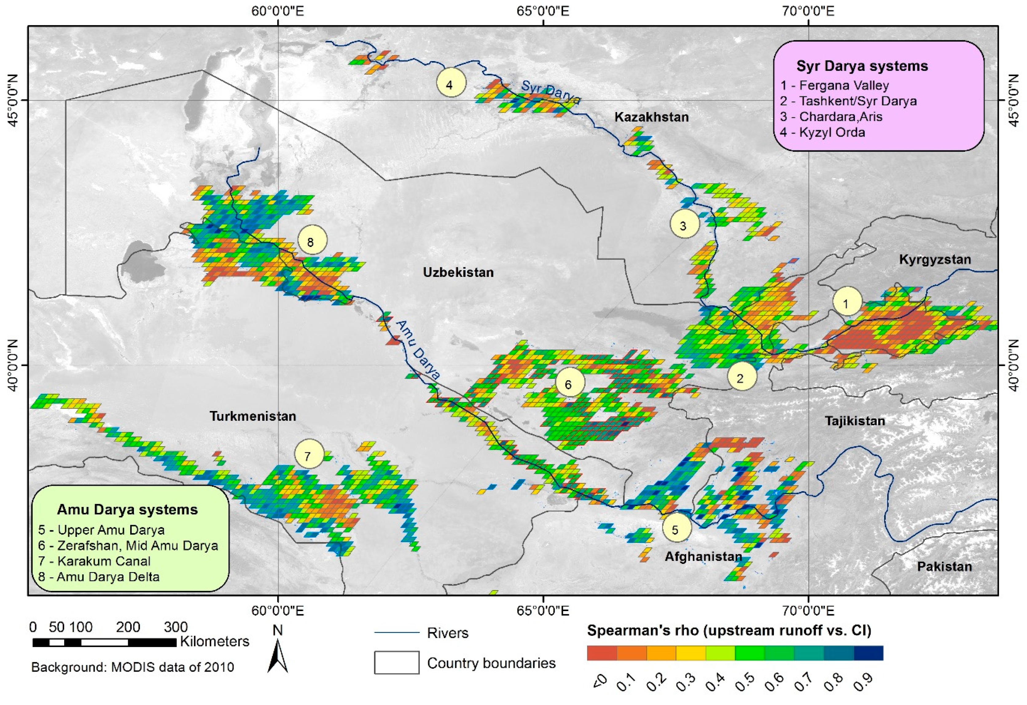
• To statistically evaluate the dependency of CI and the percentage of fallow cropland (PF) in the ASB from annual runoff formation in the upstream catchments of the Amu Darya and Syr Darya Rivers.

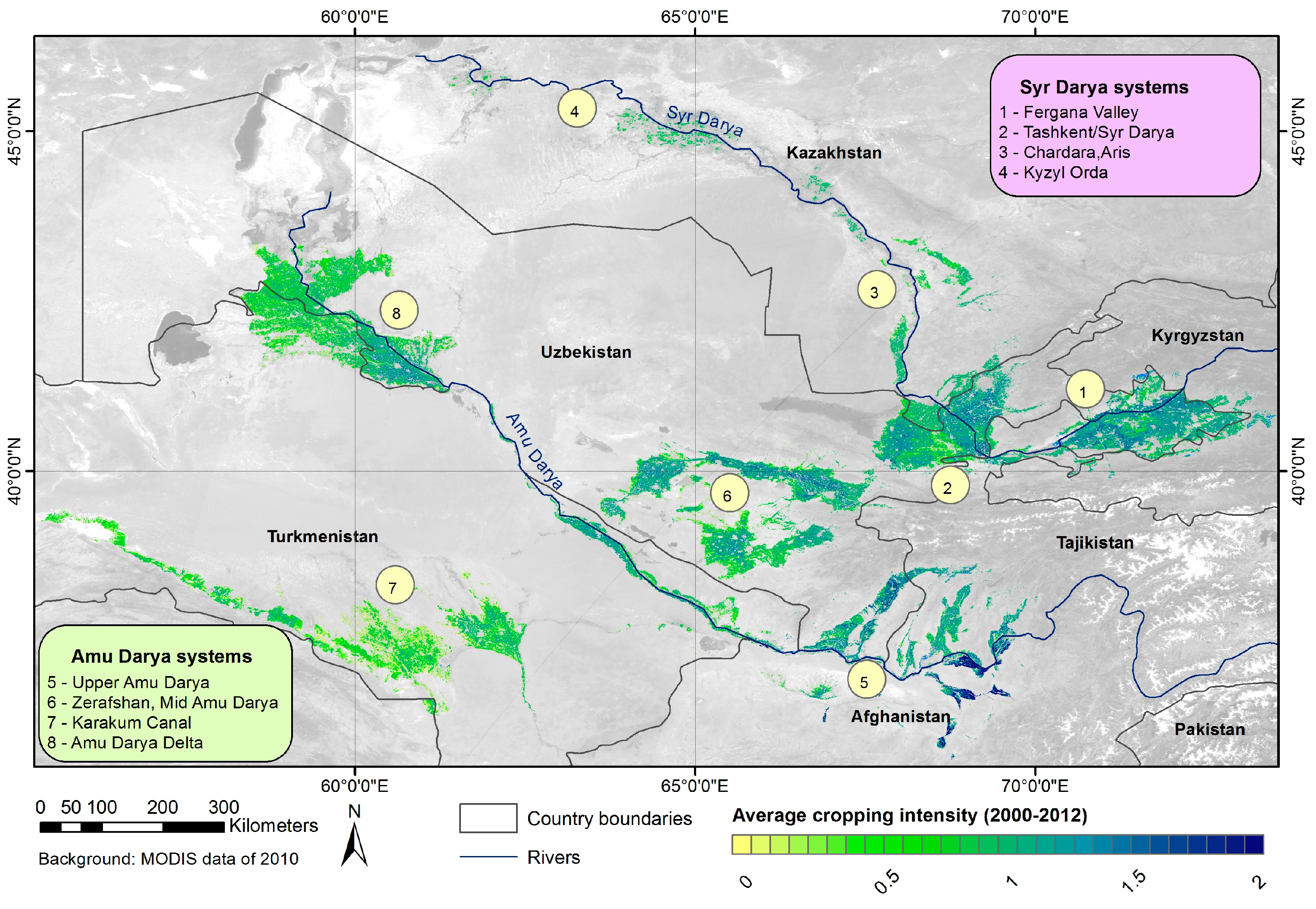
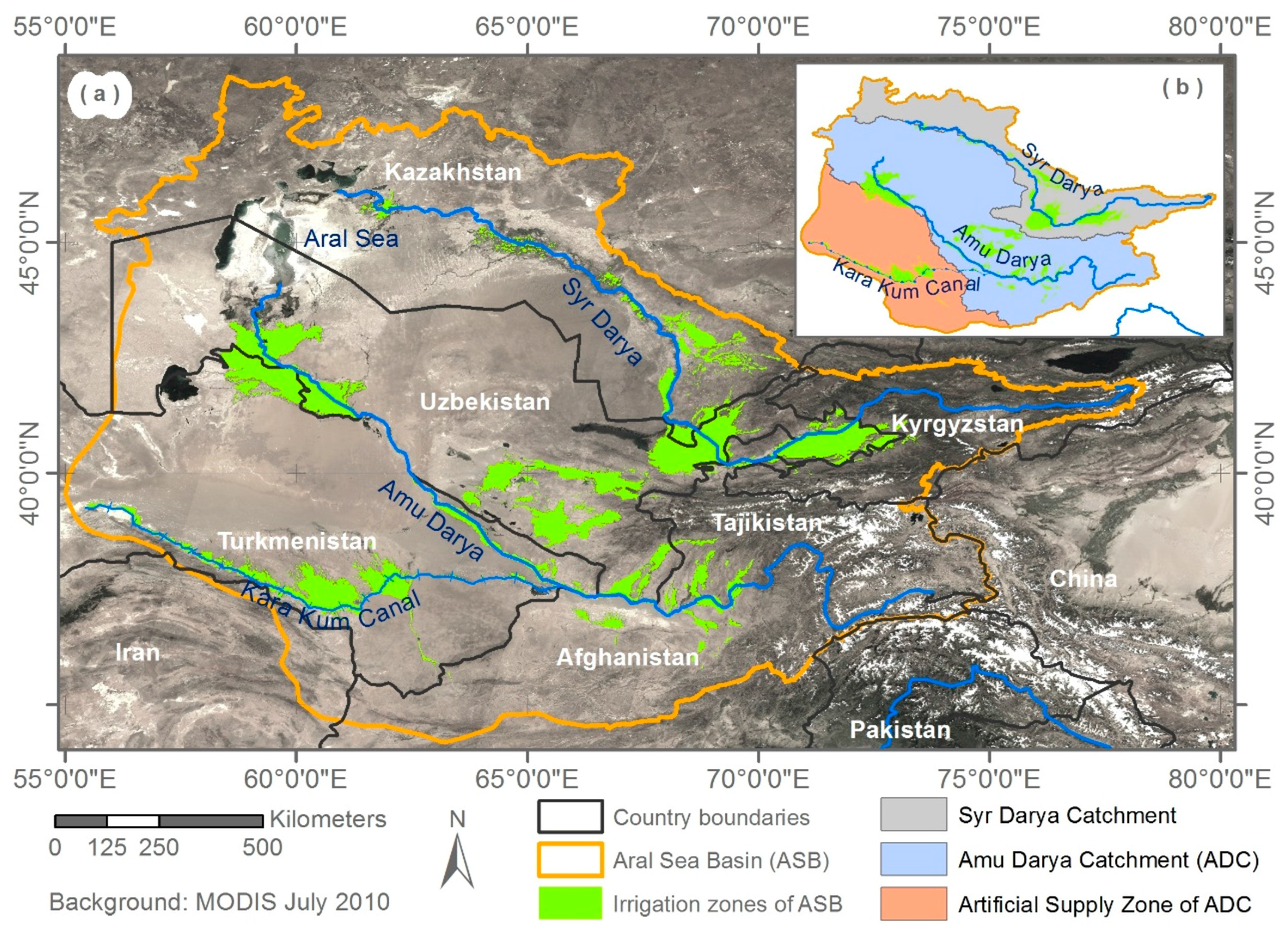
2. Study Region

The endorheic Aral Sea Basin (ASB) is located in Central Asia (Figure 1). Climate and orography divide the ASB into two parts, the extremely arid inner basin with the deserts Kyzyl Kum and Kara Kum and the semi-arid to sub-humid Tien Shan, Alai, Pamir, and Hindukush Mountains in the Southeast [1]. The major part of the water in the ASB originates from precipitation in these mountain ranges. The main receiving waters are the Amu Darya and Syr Darya Rivers (Figure 1a). Most of the fresh water in these rivers is diverted through one of the largest irrigation systems in the world [46] to ~8.5 Million ha of cropland [4]. The Kara Kum Canal on the territory of Turkmenistan conveys water through an artificial supply zone beyond the natural boundaries of the ASB [47] (Figure 1b). The water management perspective requires the inclusion of that artificial supply zone into what is called ASB. Irrigated crop production is mostly applied in the downstream countries Uzbekistan, Turkmenistan, and Kazakhstan [48]. Minor parts of the irrigated land are shared by the upstream countries Afghanistan [36], Kyrgyzstan, and Tajikistan [49]. Rainfed agriculture (winter wheat), sometimes with supplementary irrigation, only occurs upstream in the foothill regions [48]. Precipitation contributes to a minor extent to irrigated winter crop production in the eastern part of the ASB [50]. In the six countries sharing the ASB, irrigated crop production focuses on cereals (on average 49.2% of the irrigated cropland, mainly wheat, but also rice, maize, and barley), and cotton (23.2%) [51]. The share of fodder and permanent crops increases with elevation (average for all countries: 15.5%). Average field sizes reported from different case study areas throughout the ASB varied from 2.19 ha to 6.74 ha [52].

3. Materials and Methods

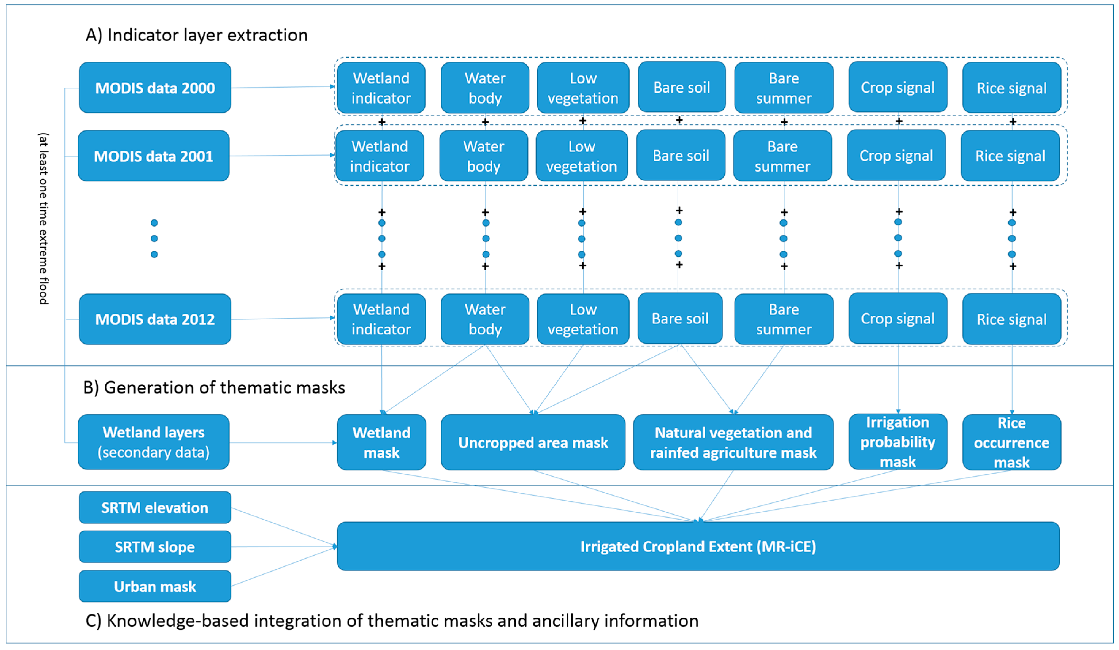
3.1. Overall Mapping Approach

Regional mapping of the moderate-resolution irrigated cropland extent (MR-iCE) was conducted based on MODIS observations of 13 years (2000–2012). Therefore, a complex rule-base including MODIS time series and secondary data was implemented. This rule-base was validated and locally optimized for reference sites using high-resolution (HR) Landsat-7 ETM+ data sets. As an intermediate step towards annual moderate-resolution cropping intensity (MR-CI) information, annual moderate-resolution cropland vegetation phenology (MR-CVP) (2000–2012) maps were derived using random forest classifications of annual MODIS time series. Multi-year, Landsat-based high-resolution cropland vegetation phenology (HR-CVP) maps were generated for training and validation of the annual MR-CVP maps. In a last mapping step, regional moderate-resolution cropping intensity (MR-CI) was composed for each observation year. The workflows are summarized in Figure 2. Figure 3 depicts the footprints of HR reference sites (based on Landsat-7) and MR (MODIS) data tiles.

To account for different cropping systems or varying ecological growth conditions in the Aral Sea Basin (ASB), eight classification zones (CZs) were introduced (Figure 3). Additionally, by implementing these CZs, the amount of applied data can be reduced and its processing can be accelerated. Each four CZs belong to the Amu Darya and Syr Darya River systems (Figure 3).

3.2. Database and Preprocessing

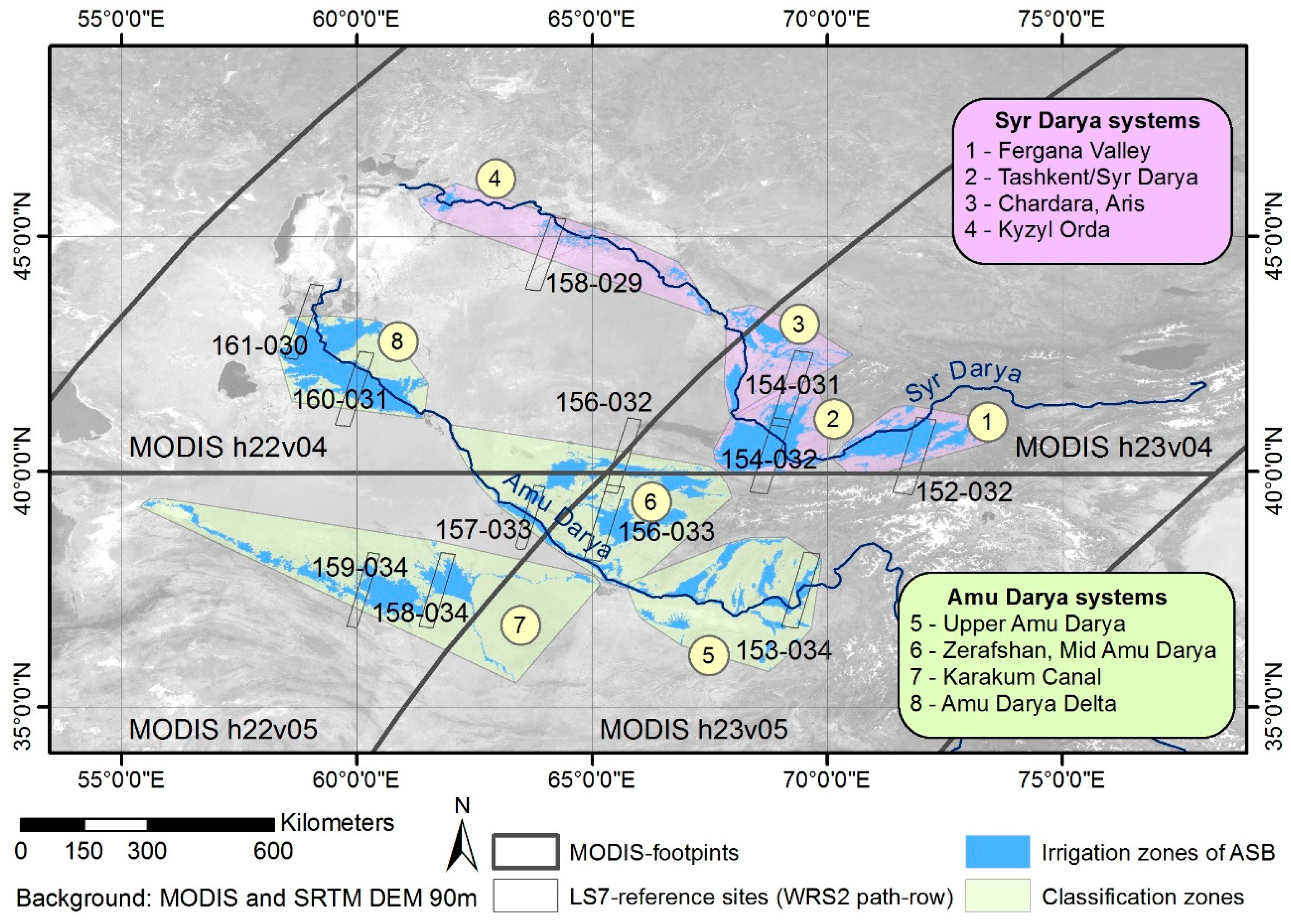
3.2.1. MODIS Data for Regional Mapping

The ASB-wide regional mapping routines were based on time series of the Normalized Difference Vegetation Index (NDVI) [53]. Therefore, 8-day 250 m Terra-MODIS surface reflectance products (MOD09Q1) were utilized.

MOD09Q1 products contain the best possible observations of the red and near infrared (NIR) bands during an 8-day period [54]. The selection considers numerous aspects such as high-observation coverage, low-view angle, the absence of clouds or cloud shadow, and aerosol content in the atmosphere. In total, four MODIS tiles (h22v04, h22v05, h23v04, h23v05) cover all irrigation planning zones in the ASB (Figure 2). For the years from 2000 to 2012, all available MOD09Q1 collection five products, i.e., 46 per year, were downloaded through the USGS Earth Explorer. An analysis of the quality of the MOD09Q1 datasets was conducted using the TiSeG software [55]. All data sets appeared as mostly undisturbed due to favorable atmospheric conditions (i.e., cloud-free and dry) and very low snow coverage in winter. Most of the remaining noise can be attributed to the situation that view angles vary among the 8-day products, even though slightly, because the algorithm for the generation of the MOD09Q1 composites selects only high quality (atmospherically undisturbed) data and with the lowest view angle [56]. High view angles (off-nadir pixels) integrate information from neighbor pixels and introduce uncertainty [57]. However, it is very likely that optimal conditions and low view angles occurred at least once at the same time during each 8-day period, as previously found for other MODIS time series analyzed in the ASB [58]. Thus, further preprocessing was omitted.

The NDVI was calculated, i.e., the difference between NIR and red reflectance was divided by the sum of the two information. Annual MODIS-NDVI time series were generated by layerstacking.

3.2.2. Landsat Data for Training and Validation

Training and validation of regional maps necessitate at least samples of HR data spatially distributed all over the study region (e.g., [33]). Due to its availability throughout 2000–2012, Landsat-7 data were selected. The ETM+ sensor provides both, 30 m multi-spectral (six bands from visible spectra to short wave infrared) and 15 m pan-chromatic data (one band from visible spectra to NIR). However, due to a technical failure onboard (scan line correction error), only a center stripe of approximately 30 km × 180 km (of originally 180 km × 180 km) is available as gapless since 2003 (USGS 2016).

In this study, Landsat-7 SLC-off data was utilized. The use of gap-filled data, i.e., data composites of different acquisitions (e.g., [59]) was assessed not to be an option because CI mapping in heterogeneous agricultural landscapes requires temporally non-shifted multi-temporal data. Atmospherically corrected Landsat surface reflectance data [60] of 12 WRS-2 (word reference system 2) tiles distributed all over the study region (Figure 3) was downloaded via the USGS Earth Explorer. The maximal possible number of cloud-free scenes per vegetation period (March–October) were acquired (

Table 1. Number of Landsat scenes available per year and reference site (named and sorted after the paths and rows of the WRS-2 tiles). From these data sets HR-iCE and HR-CVP maps were derived. The reasons for omitting single years from HR mapping are indicated by numbers in brackets and explained below the table.

CZs	Path-Row	Number of Available Scenes
		2000	2001	2002	2003	2004	2005	2006	2007	2008	2009	2010	2011	2012
1	152-32	3 (1)	5	6	5 (4)	11	12	11	11	11	7 (1)	4 (2)	6	8
5	153-34	6	4	4	2 (1)	6	6	9	10	7	6	3	8	7
3,2	154-31	3	3 (1)	3 (1)	2 (2)	8	6	6	5	6 (1)	7	5 (1)	4	7
2	154-32	3	2 (1)	4	2 (1)	6	5	5	4	5	5	6	5	7
6	156-32	3	2 (1)	4	2 (3)	8	10	6	5 (2)	5	5 (1)	4	7	6
6	156-33	4	4 (1)	4 (2)	4	9	10	9	8	7	6 (1)	9	7	5
6	157-33	4	3	3 (1)	3	8	6	6	8	4	7	7	5	9
4	158-29	4 (1)	2 (1)	3	1 (1)	8	6	6	8	4	7	7 (4)	5 (4)	9
7	158-34	3	3	3	2 (1)	6	8	6	8	7	4	6	6	2 (2)
7	159-34	2 (2)	2 (1)	2 (1)	2 (2)	8	9	9	8	9	7	9	10	11
8	160-31	3	1	2 (1)	3 (1)	5 (1)	4 (1)	8	7	8	5	6	5 (1)	8
8	161-30	2 (1)	2 (1)	2 (1)	2 (1)	7	9	5	8	7	5	4	4	8

⁽¹⁾ no spring data; ⁽²⁾ no data of early summer; ⁽³⁾ no data of late summer; ⁽⁴⁾ other problems (clouds, unsatisfying overlap of scene centers).

). The narrow footprints of the resulting Landsat reference sites in Figure 3 outline the non-gapped data of the Landsat-7 SLC-off products.

Annual layerstacks of Landsat-NDVI (2000–2012) and panchromatic data (2000, 2006, and 2012) were composed for each tile in order to derive maps on high-resolution irrigated cropland extent (HR-iCE) and high-resolution cropping intensity (HR-CI), respectively (Figure 2). Altogether, 880 Landsat scenes were processed (Table 1). Mostly due to insufficient data records (e.g., crop seasons were not covered; Table 1), 133 Landsat scenes were discarded from further analyses.

3.2.3. Secondary Data

Vector information of the irrigation planning zones for deriving the CZs (Section 3.1.) were obtained from the Scientific Information Center of the Interstate Commission on Water Coordination in Central Asia (SIC ICWC). Other secondary data were consulted for excluding implausible pixels from the MR-iCE mask. In order to mask out the settlements (Figure 2), which are typically rural, i.e., houses with gardens that easily cause spectral confusion with cropping areas in RS based mapping routines, Open Street Map (OSM) settlement layers (© OpenStreetMap contributors) were downloaded and complemented with manual digitization using Google Earth (GE). The OSM polygons of the category ‘place’ labelled as ‘city’, ‘town’, ‘village’, and ‘hamlet’ were selected. In GE, the latest available high resolution image was selected as reference for manual digitization. Last access to GE for this step was on 15 February 2016. To avoid misclassifications due to spectral confusion between crop classes and wetlands (reed covered, swamp like regions), an existing wetland layer of inner ASB [61] was enhanced with a vector data set also generated using GE. Two GIS-based terrain features, altitude and slope inclination, were derived from the DEM from the Shuttle Radar Topographic Mission (SRTM [62]) in a spatial resolution of 90 m × 90 m to identify areas topographically unsuitable for irrigation.

To assess the impact of the upstream runoff formation on the MR-CI, annual runoff data for the upstream catchments of the rivers Amu Darya and Syr Darya were acquired. They are available through the CAREWIB-portal [63]. In detail, for the irrigation systems flanking the Syr Darya (CZs 1–4), runoff information upstream the Toktogul and Andijan Reservoirs were analyzed. For the smaller rivers also feeding the Syr Darya no information was available. Runoff formation in the headwater region of the Amu Darya (CZs 5–8) was represented by inflow into the Nurek Reservoir and upstream-flow into the Panj River summarized for all hydrological years 2000–2012 (Figure 4).

3.3. Derivation of the Irrigated Cropland Extent

3.3.1. Local Scale Reference Data (HR-iCE)

To validate the regional MR-iCE, irrigated cropland extents of the reference sites were derived from Landsat data (Figure 2). In accordance with the MR-iCE, the HR-iCE should show all areas, which were used for irrigated crop production 2000–2012. Three sample years were selected assuming that every field was at least irrigated once during these time steps. To assure the inclusion of major changes of the iCE during the observation period, the years 2000, 2006, and 2012 were chosen. For each of the years, layers of pan-chromatic ETM+ data were stacked and segmented using the ENVI feature extraction tool. Target classes were cropland and other land cover types (i.e., water, settlements, bare, natural vegetation). A majority vote was applied to the overlapping area of the three masking results. For instance, if a polygon was classified as irrigated cropland two times out of the maps of 2000, 2006, and 2012, or more, it was finally assigned to the class irrigated cropland, otherwise not. For each, irrigated cropland and non-cropland, 100 samples were taken from Google Earth (using data sets of 2000–2012, in some locations only younger data were available) in order to generate a large dataset to be implemented into the mapping approach. Each HR-iCE map was optimized in case the overall accuracy of the 100 samples was 90% or below.

3.3.2. Regional Scale Mapping (MR-iCE)

The task of iCE mapping was to separate irrigated agriculture from all other land use types. Visual pre-analysis of selected annual NDVI time series within the period 2000–2012 showed the necessity of including the entire observation period of data and confirmed that using one or two years of information only is supposed to be misleading for iCE mapping [28]. The results of the pre-analysis are available in Supplementary Materials Section 1 (Figure S1).

Thus, to run the regional rule-based MR-iCE mapping (Figure 2), all 13 annual MODIS-NDVI times series (2000–2012) were analyzed. A three-step approach was implemented (Figure 5).

Extraction of Indicators

In a first step, annual MODIS-NDVI time series served to derive indicators for (i) non-irrigated areas (wetland, water, bare soil, low vegetation but no crop); for (ii) rainfed agriculture and natural vegetation of mountainous areas (bare summer); and (iii) for irrigated cropland (potential crop signal, rice occurrence) for each CZ. The rules for generating the indicators are available in Supplementary Materials Section 2 (Table S1).

Generation of Thematic Masks

Afterwards (second step), the indicator layers were summarized to thematic binary masks (Figure 5) according to the following rules:

• If the total of wetland signals amounted to more than 10 years of the observation period (2000–2012), the respective pixel became part of the wetland mask, i.e., the raster value was set to 1. The wetland mask also included available secondary data (Section 3.2.3).
• A pixel was added to the uncropped area mask, if indication for either a water body, bare soil, or low vegetation was given throughout the observation period (2000–2012).
• If natural vegetation in the mountainous regions/winter wheat (spring peak & bare summer) or bare land were mapped in the indicator layers for the entire observation period, the pixel was included in the natural vegetation & rainfed agriculture mask.
• If the total of the crop signal layer (one high vegetation period indicating a crop signal in the annual MODIS-NDVI layerstack) amounted to 0, irrigation probability mask was also set to 0.
• In the KyzylOrda and the upper Amu Darya (Afghanistan, Tajikistan) regions, the discrimination between rice and wetland became possible by analyzing the 13 rice signal indicator layers (the rules are given in Table S1). All pixels where a rice signal occurred at least once within the observation period were assigned to the rice occurrence mask.

Knowledge-Based Data Integration

In a third step, all thematic masks and further information from relevant secondary data were integrated for the derivation of the MR-iCE 2000–2012 (Figure 5). All pixels above the threshold values for the terrain attributes (slope inclination and altitude, Supplementary Materials Section 3, Table S2) were excluded in the same manner as settlements (urban mask), wetlands, uncropped area (water, soil, low vegetation), natural vegetation in mountainous regions including rainfed agriculture, as well as area with an irrigation probability of 0. All remaining pixels plus those pixels identified as rice cropping system belonged to MR-iCE.

The modeling accuracy of the MR-iCE was evaluated at a per-pixel basis. Therefore, for each, cropland and non-cropland, 100 pixels of the HR-iCE masks were aggregated to MODIS pixel size by implementing a majority rule and afterwards compared to HR-iCE for each Landsat reference site (Section 3.3.1). The overall accuracy was extracted from the confusion matrices by dividing the diagonal sum by the total number of observations [64].

3.4. Derivation of the Cropping Intensity

The regional cropping intensity (MR-CI) was mapped based on MR-CVP classifications (Figure 2). The CVP classes distinguish between ‘winter crop’ (in the ASB winter wheat predominates), ‘summer crop’ (cotton, rice, maize, sorghum, sunflower), ‘double crop’ (two crop cycles, wheat followed by a summer crop), ‘perennial & fodder crop’ (fruit tree plantations, vines, or alfalfa), ‘low vegetation’ (fields covered with herbaceous vegetation or shrubs or fields that were cropped but given up at an early stage of the season due to reduced water availability), and ‘bare land’. Cotton cannot be grown in rotation with wheat due to its long growing period.

3.4.1. Local Scale Reference Data (HR-CVP)

Knowledge-based decision trees were established to compute gridded maps on the six CVP classes, and water. Based on regional knowledge from previous mapping studies in the ASB (e.g., [31,35,65,66]), Landsat 30 m NDVI profiles were categorized using the ENVI decision tree tool, as shown in Figure 6.

Only those years could be processed, for which cloud-free information of at least three periods were available: the period of winter crops (April and May), the harvest period of winter crop enabling the differentiation between perennial & fodder crops and other crops (June and early July), and the summer crop period (August and September). Due to incomplete coverage of the cropping seasons, HR-CVP could not be processed for respective Landsat tiles of few years (respective information can be found in Table 1).

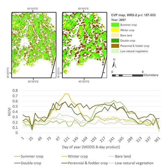
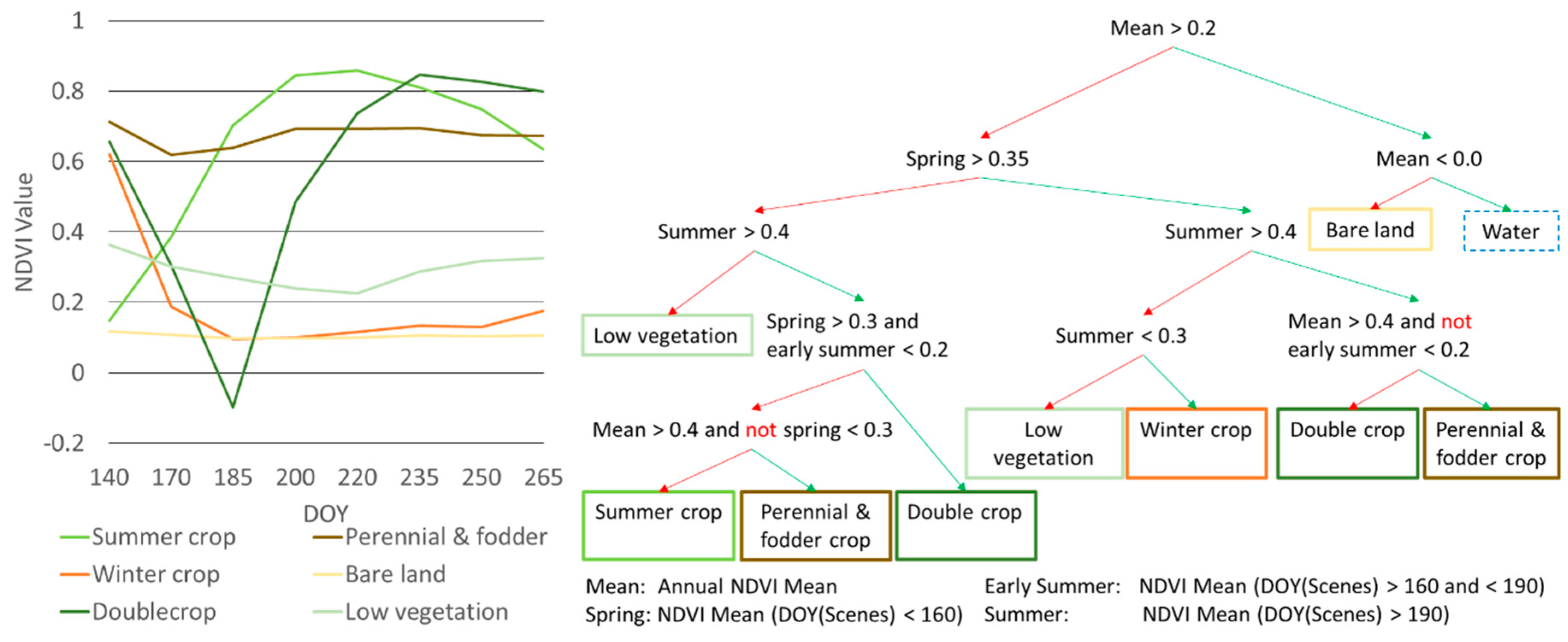
3.4.2. Regional Scale Mapping (MR-CVP)

The HR-CVP maps were aggregated to the MODIS scale using a majority vote, i.e., MR-CVP reference pixels were labelled with the class for which most HR-CVP pixels occurred. For each available HR-CVP data set and year, approximately 100 of these CVP samples were randomly selected for each class. These sample pixels were visually inspected for plausibility based on expert knowledge and existing crop classifications (e.g., [65,66]). Non-matching pixels (e.g., those clearly showing two vegetation peaks but labeled as winter crop only) were omitted from the references list. Such mismatches resulted most likely from a mixture of uncertainties in the HR-CVP maps (it could happen that important phenological features could not be detected via the available Landsat temporal coverage) and geometric displacements between Landsat and MODIS data. Ideal example NDVI time series of the six CVP classes are shown in Figure 7.

The basic algorithm used in this study is random forests (RF)—an ensemble of randomized CART decision trees [67], which proved to be a powerful prediction and analysis technique in numerous RS applications [68,69] and for mapping campaigns in irrigation systems (e.g., [43]). Therefore, the ‘randomForest’ package [70] of the R Project for Statistical Computing (R 3.2.0) [71] was applied.

First, annual RF models were built by classifying MODIS time series on an annual basis in each CZ. This step was applied only for years with reference samples (see

Table 2. Number of years, for which Landsat-7 ETM+ reference data was available for generating a HR map. Samples of CZs 2 and 3 were merged due to the comparable low number of reference data sets in CZ 3.

Classification Zones	1	2 & 3	4	5	6	7	8
	Fergana	Tashkent/Syr Darya and Chardara, Aris	Kyzyl Orda	Upper Amu Darya	Zerafshan	Karakum Canal	Amu Darya Delta
No. of years	9	11	8	12	12	12	10

). Default settings were selected for the RF models [70] and 500 regression trees were constructed with a maximal node size of five. One-third of the total number of predictors were randomly selected at each split.

The annual MODIS-NDVI time series consisted of each 46 layers. These layers served as basic features for classification. However, crop phenology can easily vary within an irrigated landscape, e.g., due to varying water availability, occurrence of late frosts, the use of different crop varieties, or other management issues. This may be not an issue as long as the reference data covers the entire spectral and phenological variability in a study region. However, the inclusion of metrics of temporal segments, i.e., average, standard deviation, minimum, maximum, or range of consecutive NDVI time steps, can account for such phenological variations in time and space, and hence, improve irrigated crop maps. These NDVI metrics were calculated for time series segments of different length. Beside the entire time series (length of the temporal segment = 46), it was divided in two (23), three (15), four (11), five (9), six (7), seven (6), nine (5), eleven (4), 15 (3), and 23 (2) parts. The metrics were calculated and added to the features space. The temporal segmentation is described in detail by Conrad et al. [65].

For measuring the accuracy of the annual models, the CVP samples of each class (Section 3.4.1) were randomly divided into training (70%) and validation (30%) samples. The validation samples served for computing the confusion matrices in a classical accuracy assessment [64].

Second, one ‘multi-annual RF model’ for each CZ was constructed out of all existing training data sets (Section 3.4.1). This multi-annual model was applied to the MODIS feature data sets of the Landsat data gaps, i.e., years without annual HR-CVP maps and consequently without annual RF model. To assess the quality of the multi-annual model, the existing annual validation data was compared to the output of the multi-annual RF model.

The final MR-CI maps consist of ‘fallow’ (bare land and low vegetation), ‘single crop’ (winter crop, summer crop, perennial & fodder crop), and ‘double crop’.

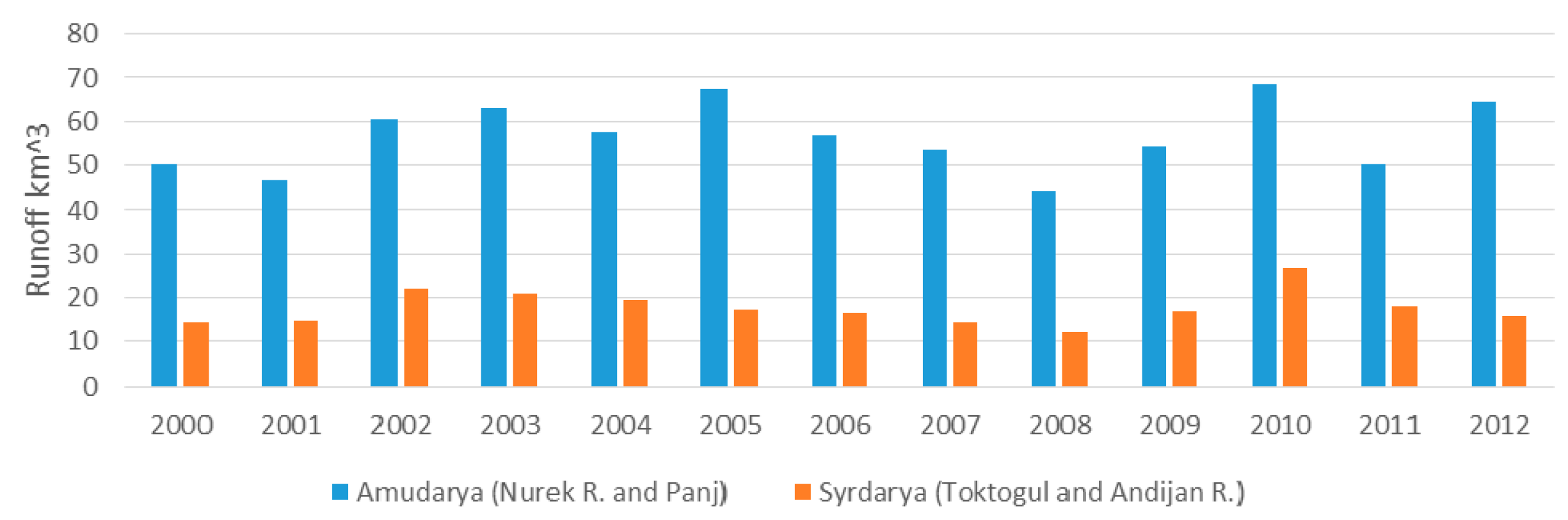
3.5. Cropping Intensity and Upstream Runoff Formation

The second aim of this study was to identify sectors in the irrigation systems of the ASB, which are affected by reduced water availability and to distinguish them from other, more independent situations. The annual information on MR-CI (2000–2012; n = 13) was spatially aggregated into grids of 10 km × 10 km (CI_GRID), i.e., each cell comprised maximal 4000 MODIS pixels. The PF was received by dividing the number of pixels mapped to be unused in the year of observation (CI = 0) by the number of pixels belonging to the MR-iCE (within a grid cell). Only cells with more than 200 MR-iCE pixels were included.

Both indicators were correlated with data on runoff formation in the upstream catchments of the rivers Amu Darya and Syr Darya. Therefore, it was hypothesized that one grid cell directly depends on upstream water availability, if CI_GRID (PF) monotonously increases (decreases) with runoff formation. Thus, for assessing the relationship between CI_GRID (PF) and upstream runoff formation, Spearman’s rho rank correlation (two-tailed t-statistics) was applied.

4. Results

4.1. Validation of Classification

The overall accuracies (OAs) of the annual MODIS-based moderate-resolution irrigated cropland extent (MR-iCE) modeled using the local Landsat high-resolution irrigated cropland extent (HR-iCE) maps varied among the classification zones (CZs) between 0.82 and 0.94 (

Table 3. OA of the MR-iCE received in the different reference sites (labelled by the WRS-2 paths and rows, ordered by the respective classification zone, CZ), plus (i) the area extents of the Landsat-based HR-iCE; (ii) the HR-iCE aggregated to MODIS pixel size; and (iii) MR-iCE received for the reference sites, as well as area comparisons between (i) and (ii), and (ii) and (iii). Comparatively high deviations from the average are given in bold numbers. Combined information on the geographic location of the reference sites and the classification zones (CZ) is given in Figure 3.

Reference Site	CZ	Overall Accuracy	Landsat Area (ha)	MODIS (Aggregated) Area (ha)	MODIS Area (ha)	MODIS (Aggregated) vs. Landsat	MODIS (Classified) vs. MODIS (Aggregated)
152-32	1	0.82	88,105	88,077	103,933	1.00	1.18
154-32	2	0.84	181,459	183,912	151,656	1.01	0.82
154-31	3	0.85	32,514	33,839	40,536	1.04	1.20
158-29	4	0.70	11,829	11,080	6903	0.94	0.62
153-34	5	0.88	43,629	44,596	51,754	1.02	1.16
156-32	6	0.91	15,293	15,040	21,816	0.98	1.45
156-33	6	0.94	93,468	92,579	107,153	0.99	1.16
157-33	6	0.86	36,926	40,579	46,859	1.10	1.15
159-34	7	0.87	64,130	67,033	91,434	1.05	1.36
158-34	7	0.87	69,450	69,078	99,000	0.99	1.43
160-31	8	0.88	68,654	72,570	84,888	1.06	1.17
161-30	8	0.82	103,302	105,937	112,224	1.03	1.06

). With a distinctly lower overall accuracy (OA) of 0.70, modeled MR-iCE for CZ 4 presents an outlier compared to the results for the further CZs. Since for each of the HR-iCE maps the same number of reference samples was tested (100 irrigated, 100 non-irrigated), the average OA of 0.85 can be used as accuracy estimation for the entire study area.

A comparison among the HR-iCE, the area of HR-iCE after the aggregation to the MODIS pixel size, and the MR-iCE for the different reference sites is given in Table 3. Aggregation of the HR-iCE to the MODIS pixel scale did not noticeably alter the mapped irrigated area (Table 3, second last column). The area classified as irrigated (MR-iCE) in most cases exceeded that of the aggregated reference data by a factor between 0.82 and 1.20 (Table 3). With 0.62, the deviations between classified MR-iCE and aggregated HR-iCE was lowest in the smallest zone CZ 4 (Table 3, last column). The difference between classified MR-iCE and aggregated HR-iCE is highest in for Landsat reference site 156-32 in CZ 6. However, this part only amounts to 10% of the entire irrigated area used for the accuracy assessment of that zone.

OAs of the annual moderate-resolution cropland vegetation phenology (MR-CVP) from 2000 to 2012 received from the annual random forest (RF) models in the different CZs varied between 0.83 and 0.99. The average amounts to 0.91. The validation of the multi-annual RF model based on reference Landsat data returned partially lower OAs ranging from 0.70 to 0.98. This also results in a slightly lower averaged overall estimation of 0.89. In 9 cases (out of 73), the multi-annual RF model outperformed the annual RF model. The OAs for the best performing model for each CZ and year are given in

Table 4. OAs of CVP classifications (summer crop, winter crop, bare land, double crop, perennial & fodder crop, low natural vegetation) using RF models (the situation that multi-annual RF outperformed annual RF models are grey-shaded); and all validation samples of all available years with the multi-annual RF model. ‘x’ = no reference Landsat data available within this classification zone and year.

Model	Classification Zone
	1	2 & 3	4	5	6	7	8
2000	x	0.89	x	0.87	0.86	0.84	0.88
2001	0.98	x	x	0.95	x	0.89	x
2002	0.95	0.95	0.95	0.92	0.88	0.86	x
2003	x	x	x	x	x	x	x
2004	0.86	0.92	0.92	0.92	0.90	0.88	0.86
2005	0.86	0.96	0.91	0.96	0.88	0.86	0.88
2006	0.92	0.89	0.86	0.95	0.87	0.89	0.87
2007	0.96	0.93	0.89	0.96	0.98	0.91	0.89
2008	0.94	0.93	0.98	0.95	0.90	0.90	0.91
2009	x	0.93	0.91	0.93	0.91	0.92	0.91
2010	x	0.94	x	0.94	0.85	0.92	0.87
2011	0.97	0.94	x	0.92	0.88	0.99	0.92
2012	0.93	0.92	0.96	0.96	0.84	0.88	0.91
All Years Merged	0.90	0.92	0.91	0.92	0.92	0.87	0.87

. The multi-annual RF model achieved average OAs from 0.87 to 0.92 when validated against all independent reference samples from 2000 to 2012. It was applied in all situations of missing reference data (‘x’ in Table 4).

Increased OA was found after reorganizing the MR-CVP classifications to model moderate-resolution cropping intensity (MR-CI). For 23 cases (out of 73), the multi-annual RF model outperformed the annual RF model, even though slightly.

Table 5. OAs of modeled CI accounting for the number of harvests per year based on RF models (the situation that multi-annual RF outperformed annual RF models are grey-shaded); and all validation samples of all available years with the multi-annual RF model. ‘x’ = no reference Landsat data available within this classification zone and year.

Model	Classification Zone
	1	2 & 3	4	5	6	7	8
2000	x	0.97	x	0.93	0.92	0.95	0.99
2001	0.98	x	x	0.98	x	0.93	x
2002	0.96	0.99	0.98	0.97	0.90	0.93	x
2003	x	x	x	x	x	x	x
2004	0.91	0.99	0.96	0.96	0.92	0.95	0.95
2005	0.92	0.99	0.95	0.98	0.92	0.92	0.94
2006	0.95	0.95	0.94	0.98	0.97	0.96	0.93
2007	0.98	0.98	0.94	0.98	1.00	0.97	0.97
2008	0.96	0.99	1.00	0.98	0.93	0.99	0.96
2009	x	0.97	0.98	0.97	0.93	0.98	0.97
2010	x	0.98	x	0.96	0.89	0.98	0.95
2011	0.99	0.98	x	0.98	0.92	1.00	0.97
2012	0.97	0.99	0.97	0.98	0.90	0.96	0.96
All Years Merged	0.93	0.98	0.95	0.96	0.92	0.95	0.95

lists the accuracies of the best performing RF model. Validating the multi-annual RF model that was applied in situations of missing reference data returned OAs ranging between 0.92 and 0.98. With 0.92, the lowest average OA merged for all years occurred in CZ 6. None of the CZs underperformed notably.

4.2. Irrigated Cropland Extent and Cropping Intensity in the ASB 2000–2012

For the observation period from 2000 to 2012, almost all CZs in the ASB show a high coverage of MR-iCE. Only the irrigation zones in South Kazakhstan, Kyzyl Orda, and in remote areas of Turkmenistan exhibited more scattered patches of MR-iCE (Figure 8).

For the same period, annual MR-CI varies in average between 0.53 and 1.23 for the Amu Darya River and between 0.84 and 1.09 for the Syr Darya River system (

Table 6. Regional cropping intensity based on MODIS data (MR-CI) averaged over the observation period from 2000 to 2012 and for the classification zones (CZ) in the according river system.

Classification Zone (CZ)	Average MR-CI
Fergana Valley (1)	1.09
Tashkent/Syr Darya (2)	1.05
Chardara, Aris (3)	0.84
Kyzyl Orda (4)	0.86
Syr Darya River (CZ 1–4)	1.04
Upper Amu Darya (5)	1.23
Zerafshan, Mid Amu Darya (6)	0.95
Karakum Canal (7)	0.53
Amu Darya Delta (8)	0.78
Amu Dary River (CZ 5–8)	0.83

). Generally, the higher the MR-CI, the more intensive is the use of irrigated cropland. For both river systems, a general decrease of mapped annual MR-CI can be observed in upstream-downstream direction (Figure 8). For the Amu Darya, highest annual MR-CI values of approximately 2 mainly occurred in the upstream irrigation systems in Afghanistan whereas values around 1 were mapped along the Zerafshan River (northern CZ 6) in the midstream part of the Amu Darya. Lowest annual MR-CI values (<1) characterize the irrigation systems of the Karakum Canal and the western and northern Amu Darya delta. The latter (CZ 8) shows its own gradient of MR-CI in upstream-downstream direction. For the Syr Darya River, highest mapped MR-CI values around 1.5 mainly prevail in the Fergana Valley and in the region of Tashkent with few scattered plots of MR-CI below 1 in both irrigation systems. The more upstream the Syr Darya, the lower is the mapped annual MR-CI from around 1 in southern Kazakhstan to values below 1 in the rice dominated lower irrigation systems of Kyzyl Orda (Figure 8).

4.3. Cropping Intensity and Upstream Runoff Formation

Significant correlations (Spearman’s rho) with upstream runoff in the hydrological years were found for both gridded cropping intensity (CI_GRID) and percentage of fallow cropland (PF), in all CZs, also for the total MR-iCE in the Amu Darya catchment (

Table 7. Spearman’s rank correlation coefficient (Spearman’s rho) for the correlation between the upstream runoff formation and intensity indicators cropping intensity (CI_GRID) and percentage of and fallow frequency (PF) in the eight classification zones (CZ), and the entire catchment.

Syr Darya	CZ 1	CZ 2	CZ 3	CZ 4	Catchment
Upstream runoff vs. CIGRID	0.0989	0.5275	0.3901	0.5934 *	0.4176
Upstream runoff vs. PF	−0.4341	−0.6374 *	−0.4011	−0.5934 *	−0.6264 *
Amu Darya	CZ 5	CZ 6	CZ 7	CZ 8	Catchment
Upstream runoff vs. CIGRID	0.6868 *	0.5714 *	0.7088 *	0.6978 *	0.6758 *
Upstream runoff vs. PF	−0.7418 *	−0.6429 *	−0.5879 *	−0.6209 *	−0.6483 *

* Significance level > 95%.

). Runoff and CI_GRID were positively correlated, negative Spearman’s rho occurred for PF. Highest Spearman’s rho occurred for CI_GRID in Turkmenistan (CZ 7), whereas PF showed highest correlation with runoff in the upstream systems (CZ 5). In a total contrast to the Amu Darya River, both indicators do not significantly correlate to the upstream runoff in the Syr Darya river system. However, only for CZ 4 (Kyzyl Orda), the results reveal significant correlations for both indicators. Decreased strength of correlation was found for the entire catchment, and the CZs 1, 2, and 3. Upstream runoff was also significantly correlated to PF in the zones Tashkent/Syr Darya (CZ 2), and when aggregated to all MR-iCE pixels (Table 7).

The gridded results of Spearman’s rho enable to distinguishing between areas in the CZs with different dependencies between upstream runoff and CI_GRID (Figure 9). Predominating low rank coefficients occurred for instance upstream in the Syr Darya catchment, in Fergana Valley, or in the southern Amu Darya Delta. Significant correlations (Spearman’s rho >0.5549) mainly prevail in the most upstream (i.e., Tajikistan and Afghanistan) and in the most downstream Amu Darya River system, e.g., in the northern Amu Darya Delta. Along the Syr Darya River, significant correlations existed in the western Tashkent/Syr Darya region as well as in few locations in its downstream part in Kazakhstan (Figure 9).

Similar spatial patterns returned from mapping Spearman’s rho for the relationship between PF and upstream runoff (Figure 10). For instance, the statistical dependency between PF and upstream runoff was stronger in the Amu Darya catchment than in the Syr Darya catchment, where in the downstream regions (CZs 3 and 4) many grid cells showed decreased correlations. Most parts of the Fergana Valley seemed to remain uninfluenced by runoff fluctuations in terms of PF, which can be seen from the low rank correlations. However, the total number of significant rank correlations (emphasized by yellowish to reddish cells in Figure 11) was higher for PF than for CI_GRID (Figure 9, Table 7).

5. Discussion

5.1. Methodological Approach

A remote sensing (RS) based approach was implemented for mapping the regional irrigated cropland extent (iCE) and the cropping intensity (CI) at the MODIS pixel level in the Aral Sea Basin (ASB). Except for the northern ASB (classification zone (CZ) 4), the overall accuracy (OA) from the moderate-resolution irrigated cropland extent (MR-iCE) classifications ranged at the upper level of that achieved in other regional cropland mapping studies summarized by Ozdogan et al. [38]. The good performance can mainly be attributed to the cloud-free and low atmospheric water vapor conditions, which enabled an excellent database comprising (i) high-quality MODIS time series (for mapping) and (ii) multiple cloud-free Landsat data (for training and validation). In South and Southeast Asia for instance residual cloud contamination in MODIS products can highly challenge cropland mapping [23,41,42,72]. The predominating dry climate in the ASB also eased the separation between irrigated and non-irrigated agriculture in this study. In contrast, regional iCE mapping in more humid climates requires complex considerations of agro-climatic conditions to reduce misclassifications between iCE and non-irrigated cropland (e.g., [42,45]). Moreover, confusion between grassland and monocyclic cropping (summer, winter, annual crops & perennial), which is known to complicate irrigated cropland mapping in humid zones (e.g., [23,42]), was also almost irrelevant in this study.

However, similar to other iCE mapping approaches based on MODIS data (e.g., [29,45]), overestimations of area occurred. In comparison to the high-resolution irrigated cropland extent (HR-iCE) maps, some natural vegetation and rainfed agriculture were erroneously included into the MR-iCE mask. Despite thoroughly developed rule sets and corrections using manually digitized wetland layers, few wetlands were still found in the MR-iCE masks such as in the lowlands of Amu Darya and Syr Darya (CZs 3, 4, 8). Visual comparisons also revealed that in few locations the settlement masks applied to MR data underestimated the actual extent of the settlements. This in turn led to an overestimation of MR-iCE. Similar uncertainties were reported by Salmon et al. [28] from the derivation of global cropland layers. In few locations in the ASB, undervalued HR-iCE maps increased the discrepancy between the area estimates.

Figure 11 exemplifies the underestimations in HR-iCE and major errors in the urban mask. Both led to overestimations in the respective MR-iCE map. Also in the southwest of the ASB (CZ 7), confusion of MR-iCE with rural settlements was found to be the major reason for deviations from HR-iCE.

Uncertainty in area extents of regional iCE maps introduced by coarse pixel resolutions have been intensively investigated (e.g., [73,74,75]). Due to the MODIS pixel size of 250 m, those data identified as irrigated cropland can also include non-irrigated areas (e.g., roads, canals, buildings, or other land cover types). In contrast, pixels labeled as non-cropland can comprise cropland patches. Depending on the density and fragmentation of irrigated cropland, iCE classifications at the pixel level can typically underestimate and overestimate the actual cropland extent. Mapping at the sub-pixel level as for instance addressed by Thenkabail et al. [29] and Pervez et al. [36] may have led to more precise assessments. However, extensive fields and the fact that irrigated fields are usually strongly connected in one canal reach [37] make field complexes in the ASB commonly exceeding the area size of a MODIS pixel (6.25 ha). This certainly is supposed to be a reason why both, HR-iCE and HR-iCE aggregated to the MODIS scale, nearby equal in area (Table 3). It further confirms the suitability of MODIS 250 m data to approximate the actual iCE in the ASB.

Altogether, the analysis of cropland pixels confirmed previous observations and statements on the necessity of including multi-annual data into iCE mapping (e.g., [19,28,76]). Moreover, it underlined the assumption that in the ASB the use of three-year data only may be still a source for underestimations of actual iCE.

As for the MR-iCE maps, the average accuracy levels indicate the applicability of 250 m MODIS data for regional mapping of cropland vegetation phenology (CVP) and CI of the large-scale irrigation systems in the ASB. Comparison with other studies underlines the dependency of the accuracy in MODIS mapping routines from the homogeneity of the investigated agricultural landscape. Applying MODIS-based mapping, Wardlow and Egbert [40] for instance found over 10 Mio ha of cropland in Kansas, U.S., even with higher accuracy levels (e.g., for summer crops), which could be mainly attributed to the enormous field sizes of more than 6–12 MODIS pixels (and comparatively good atmospheric conditions for RS applications). On the contrary, when observing small parceled irrigated agriculture where sub-pixel approaches may be advantageous, lower correlations between subpixel area estimates and aggregated information from HR satellite data were found for instance by Jain et al. [43] for few parts of India. In such cases, it depends on the scale at which the information is required for further analysis since the area estimates with increasing size (e.g., of harvested area) commonly balance out the reference area [23,43,72].

The combination of temporal segmentation, e.g., the utilization of metrics derived from temporal segments of NDVI time series in the feature space for classification [65] with the construction of a multi-annual model allowed for adequately mapping moderate-resolution cropland vegetation phenology (MR-CVP) and moderate-resolution cropping intensity (MR-CI), at least in those years for which high resolution (HR) validation data was available. Few uncertainties remain, e.g., when transferring the multi-annual random forest (RF) model to years for which no validation data was available. However, since for each HR reference site at least eight years (out of 13) of data were available (Table 2) it can be inferred that most climatic and hydrological conditions of the entire observation period were covered and, hence, that the transferability is valid.

As Ozdogan et al. [38] state, iCE or CI for subsistence scale irrigation cannot be reported from using MODIS pixels. Even though theoretically approximations should become possible by utilizing urban footprint masks and NDVI time series, small-scale agriculture such as gardening in rural settlements, were excluded from this study as well.

5.2. Assessment of CI in the ASB (2000–2012)

The total area of MR-iCE in the ASB (2000–2012) amounts to 10.1 Mio·ha. Accounting for an average overestimation of approximately 20% from the results of annual MR-iCE (compared to the HR-iCE maps), the total irrigated area is estimated to be 8.4 Mio·ha. As reported by Bekchanov et al. [4], FAO [51], and SIC ICWC [77]) 8.5 Mio·ha, 8.19 Mio·ha, and 7.9 Mio·ha of land are reported to be actually under irrigation in the ASB. The well matching numbers hint to oversized areas in official statistics, because the area actually under irrigation’ as defined by FAO [51] refers to an annual average whereas the MR-iCE maps outline the maximal area under irrigation over a 13 year period. A second statistical indicator for the extent of irrigated cropland in the ASB, the area equipped for irrigation’, officially given to be 9.76 Mio·ha. [51], exceeds the area irrigated at least once within 2000–2012 by far. Again the comparability, which would again lead to overestimations in official statistics, can be questioned, because theoretically, there can be areas unused for irrigation over the 13 year period listed in this statistics, even though some costs for restarting irrigation may be high. However, achieving more accurate results requires a minimization of the aforementioned technical uncertainties, or simply another approach, e.g., manual digitization or the area-wide utilization of Landsat. This, however, is assumed to be very time- and also cost-consuming, thus to be unfeasible for a regional approach. It has to be noted that these sources of uncertainty of course affect the subsequently derived CVP, CI, and percentage of fallow cropland (PF), also. The focus of this study was on regional estimations of cropping intensity parameters and their statistical relation to upstream runoff formation rather than on locally accurate measurements of the respective information.

Also, comparisons between the observed MR-CI and official statistics remain speculative, because official information on CI was only available at the national level [51] rather than at the catchment scale for certain irrigation systems in the ASB. Only a CI below 0.5 observed in the entire CZ 7 and the Turkmen part of CZ 8 obviously disapproves those 1.01 given by FAO. Intensified double cropping as registered in the Afghan part of CZ 5 confirmed the results by Pervez et al. [36].

The observed MR-CI values varied intensively among the years. Furthermore, for large areas in the Amu Darya catchment, they significantly depend on upstream runoff formation. Statistical connection indicated a decreased, or even no dependency on upstream runoff formation in the Syr Darya catchment. There, only for the comparatively small downstream Kyzyl Orda region (CZ 4), similar agreements between CI and upstream runoff was found. This difference is assumed to result from the number of regulation constructions (e.g., dams) along the Syr Darya, which is higher compared to the Amu Darya [4]. For the course of the Amu Darya, the Tuyamuyun Reservoir with a total volume of approximately 4.5 km³ is stated to be the only remarkable artificial water storage [78]. However, its impact is indicated by the comparatively high MR-CI values in its upstream locations of CZ 8 leading to a second gradient of CI in the river system (Figure 8).

The PF showed significant strong relations with upstream runoff in both river systems, whereas for the Syr Darya, national upstream-downstream disparities of that relation become visible. The CZs 1 and 2 mostly belong to Uzbekistan, and CZs 3 and 4 are located in Kazakhstan. In both countries, significant correlations occurred in the more downstream irrigation zones only (CZs 2 and 4). Figure 12 highlights this national differences of inter-annual development of CI at the example of CZ 2. The southern and northern parts depict the downstream situation in Uzbekistan and the upstream locations in Kazakhstan, respectively. The country border would be visible (in most of the years) even by the different cropping patterns only. In South Kazakhstan, one harvest was reaped regularly and summer crops predominated according to the MR-CVP maps. Two harvests regularly occurred in the Uzbek part of that CZ, but particularly in years after drought situations (2002, 2009, see Figure 4). Drought situations as in 2001 or 2008 [6] increased PF (and reduced CI).

The intensified double cropping observed through RS reflects the necessity of Uzbekistan for using the irrigation systems for winter wheat production, for which Kazakhstan utilizes its extensive steps in the North of the country [48]. The intra-annual variability of CI also underlines the strong dependency of Uzbekistan from irrigation water. This dependency is also visible in the Spearman’s rho (CI_GRID or PF vs. runoff formation) observed in South Kazakhstan (Figure 12), but the visual impression suggests that it occurred on a lower level. This points at one methodological challenge of using Spearman’s rho that permitted making conclusions about the monotony of the relationship between land use and runoff formation rather than about the actual shape of the relationship (its linearity of its range of values).

The interrelations of CI (or PF) with upstream runoff formation in the 10 km × 10 km grid (Figure 9 and Figure 10) pointed at both locations independent from natural processes, suggesting either a continuously high or low CI. The latter can be observed through the MR-CI maps (Figure 8). For instance, in the Amu Darya Delta (CZ 8), CI was comparatively high in the southern part (Khorezm, see also [63,65], and low in the eastern Turkmen parts. However, neither locations showed signs of dependency from upstream runoff in CI in contrast to the downstream locations of that zone, or the desert fringe in the most southern parts of that CZ. For the Khorezm region, again impact of the Tuyamuyun Reservoir is indicated, whereas high soil salinity, which affects nearby all cropland in Turkmenistan [51] and in particular that part of the Amu Darya Delta [79], may be a plausible explanation for the reduced use of cropland there and for the reduced CI in CZ 7.

Also within the different irrigation systems (at the local scale), numerous factors such as water distribution problems, which occur at different scales and may range from infrastructure problems [1,2] to political, social, and institutional challenges [6,80,81], soil salinity and shallow groundwater [12,14], or other reasons can influence CI and PF. However, this cannot be clarified in this study. The results show that and where interdependencies between runoff formation and CI occurred and where other reasons need to be investigated to explain the observed land use patterns, which in turn may be used for targeted further analysis aiming at the planning of improvement measures.

6. Conclusions

This study presents a novel method for assessing cropping intensities in the irrigation systems of the Aral Sea Basin in Central Asia. Utilizing MODIS data and ancillary spatial data (urban layers, spatial maps of natural vegetation classes) allowed for accurately assessing relevant agricultural parameters, i.e., irrigated cropland extent, cropland vegetation phenology and cropping intensity in the Aral Sea Basin. Gradients of cropping intensity and impacts of water regulation became visible during the observation period 2000–2012. Cropping intensity can now be aggregated over several years, e.g., to investigate double cropping systems, fallow sequences, or to monitor processes of production change, e.g., land abandonment.

Several factors promoted the applicability of the mapping approach for broad-scale agricultural monitoring in the study region: the agricultural system (extensive fields, low diversity of crops, and simple cropping calendars), the favorable atmospheric conditions, the continental climate, and the access to ancillary data. The methods may thus be applied beyond the Aral Sea Basin in similar cropping systems and ecological conditions (e.g., in parts of the Mid East). A transfer of the methods to small scale agriculture systems or to humid climate zones remains challenging due to increased efforts of data handling and class legends.

However, high classification accuracies revealed by the applied mapping approach were crucial to further asses the relationship between annual runoff formation in the upstream catchments of the Amu Darya and Syr Darya Rivers and two parameters, the cropping intensity and the percentage of fallow cropland. Especially in the Amu Darya catchment, a strong impact of upstream runoff formation to downstream cropping intensity was identified. Impacts of flow regulation became visible in the Amu Darya Delta only. The reduced relationship between upstream runoff and cropping intensity along the Syr Darya may be attributed to regulation constructions such as artificial dams. It may also be the result of lower total water demand for agriculture in the catchment, or other explaining factors.

The results enable identifying spatial disparities of the impact of runoff formation and thus provide an analytical instrument for regional, transboundary management, and planning. The spatially explicit information is important to assess socio-economic and environmental causes of intensification or de-intensification of agricultural production in the region, and to modify these processes, among others, in increasing economic and ecological sustainability in the Aral Sea Basin. The acquirements can be also utilized for investigating the effects of irrigated agriculture on the hydro-climatic cycle in the region, such as local cooling caused by evapotranspiration, or increased water vapor dynamics in the atmosphere.

References

1. Micklin, P. The aral sea disaster. Annu. Rev. Earth Planet. Sci. 2007, 35, 47–72. [Google Scholar] [CrossRef]
2. Cai, X.; McKinney, D.C.; Rosegrant, M.W. Sustainability analysis for irrigation water management in the Aral Sea region. Agric. Syst. 2003, 76, 1043–1066. [Google Scholar] [CrossRef]
3. Siegfried, T.; Bernauer, T.; Guiennet, R.; Sellars, S.; Robertson, A.W.; Mankin, J.; Bauer-Gottwein, P.; Yakovlev, A. Will climate change exacerbate water stress in Central Asia? Clim. Chang. 2012, 112, 881–899. [Google Scholar] [CrossRef]
4. Bekchanov, M.; Ringler, C.; Bhaduri, A.; Jeuland, M. Optimizing irrigation efficiency improvements in the Aral Sea Basin. Water Resour. Econ. 2015, 13, 1–16. [Google Scholar] [CrossRef]
5. Chemin, Y.; Platonov, A.; Ul-Hassan, M.; Abdullaev, I. Using remote sensing data for water depletion assessment at administrative and irrigation-system levels: Case study of the Ferghana Province of Uzbekistan. Agric. Water Manag. 2004, 64, 183–196. [Google Scholar] [CrossRef]
6. Tischbein, B.; Manschadi, A.M.; Conrad, C.; Hornidge, A.-K.; Bhaduri, A.; Ul Hassan, M.; Lamers, J.P.A.; Awan, U.K.; Vlek, P.L.G. Adapting to water scarcity: Constraints and opportunities for improving irrigation management in Khorezm, Uzbekistan. Water Sci. Technol. Water Supply 2013, 13, 337–348. [Google Scholar] [CrossRef]
7. Thevs, N.; Ovezmuradov, K.; Zanjani, L.V.; Zerbe, S. Water consumption of agriculture and natural ecosystems at the Amu Darya in Lebap Province, Turkmenistan. Environ. Earth Sci. 2014, 73, 731–741. [Google Scholar] [CrossRef]
8. Bichsel, C. Liquid challenges: Contested water in central. Sustain. Dev. Law Policy 2011, 12, 24–30. [Google Scholar]
9. Lioubimtseva, E.; Henebry, G.M. Climate and environmental change in arid Central Asia: Impacts, vulnerability, and adaptations. J. Arid Environ. 2009, 73, 963–977. [Google Scholar] [CrossRef]
10. Mannig, B.; Müller, M.; Starke, E.; Merkenschlager, C.; Mao, W.; Zhi, X.; Podzun, R.; Jacob, D.; Paeth, H. Dynamical downscaling of climate change in Central Asia. Glob. Planet. Chang. 2013, 110, 26–39. [Google Scholar] [CrossRef]
11. Schlüter, M.; Leslie, H.; Levin, S. Managing water-use trade-offs in a semi-arid river delta to sustain multiple ecosystem services: A modeling approach. Ecol. Res. 2009, 24, 491–503. [Google Scholar] [CrossRef]
12. Qadir, M.; Noble, A.D.; Qureshi, A.S.; Gupta, R.K.; Yuldashev, T.; Karimov, A. Salt induced land and water degradation in the Aral Sea basin: A challenge to sustainable agriculture in Central Asia. Nat. Resour. Forum 2009, 33, 134–149. [Google Scholar] [CrossRef]
13. Khamzina, A.; Lamers, J.P.A.; Vlek, P.L.G. Tree establishment under deficit irrigation on degraded agricultural land in the lower Amu Darya River region, Aral Sea Basin. For. Ecol. Manag. 2008, 255, 168–178. [Google Scholar] [CrossRef]
14. Dubovyk, O.; Menz, G.; Khamzina, A. Land suitability assessment for afforestation with Eleagnus Angustifolia L. in degraded agricultural areas of the lower Amu Darya Basin. L. Degrad. Dev. 2014. [Google Scholar] [CrossRef]
15. Lobell, D.B.; Bonfils, C.J.; Kueppers, L.M.; Snyder, M.A. Irrigation cooling effect on temperature and heat index extremes. Geophys. Res. Lett. 2008, 35, 1–5. [Google Scholar] [CrossRef]
16. Sorooshian, S.; Li, J.; Hsu, K.L.; Gao, X. How significant is the impact of irrigation on the local hydroclimate in Californias Central Valley? Comparison of model results with ground and remote-sensing data. J. Geophys. Res. Atmos. 2011, 116, 1–11. [Google Scholar] [CrossRef]
17. Wen, L.; Jin, J. Modelling and analysis of the impact of irrigation on local arid climate over northwest China. Hydrol. Process. 2012, 26, 445–453. [Google Scholar] [CrossRef]
18. Douglas, E.M.; Beltrán-Przekurat, A.; Niyogi, D.; Pielke, R.A.; Vörösmarty, C.J. The impact of agricultural intensification and irrigation on land-atmosphere interactions and Indian monsoon precipitation—A mesoscale modeling perspective. Glob. Planet. Chang. 2009, 67, 117–128. [Google Scholar] [CrossRef]
19. Siebert, S.; Portmann, F.T.; Döll, P. Global patterns of cropland use intensity. Remote Sens. 2010, 2, 1625–1643. [Google Scholar] [CrossRef]
20. Monfreda, C.; Ramankutty, N.; Foley, J.A. Farming the planet: 2. Geographic distribution of crop areas, yields, physiological types, and net primary production in the year 2000. Glob. Biogeochem. Cycles 2008, 22, 1–19. [Google Scholar] [CrossRef]
21. Portmann, F.T.; Siebert, S.; Döll, P. MIRCA2000—Global monthly irrigated and rainfed crop areas around the year 2000: A new high-resolution data set for agricultural and hydrological modeling. Glob. Biogeochem. Cycles 2010, 24, 1–24. [Google Scholar] [CrossRef]
22. Conrad, C.; Loew, F.; Rudloff, M.; Schorcht, G. Assessing irrigated cropland dynamics in central Asia between 2000 and 2011 based on MODIS time series. Proc. SPIE 2012. [Google Scholar] [CrossRef]
23. Gray, J.; Friedl, M.; Frolking, S.; Ramankutty, N.; Nelson, A.; Gumma, M.K. Mapping Asian cropping intensity with MODIS. IEEE J. Sel. Top. Appl. Earth Obs. Remote Sens. 2014, 7, 3373–3379. [Google Scholar] [CrossRef]
24. Ganguly, S.; Friedl, M.A.; Tan, B.; Zhang, X.; Verma, M. Land surface phenology from MODIS: Characterization of the Collection 5 global land cover dynamics product. Remote Sens. Environ. 2010, 114, 1805–1816. [Google Scholar] [CrossRef]
25. Ramankutty, N.; Evan, A.T.; Monfreda, C.; Foley, J.A. Farming the planet: 1. Geographic distribution of global agricultural lands in the year 2000. Glob. Biogeochem. Cycles 2008. [Google Scholar] [CrossRef]
26. Waldner, F.; Fritz, S.; Di Gregorio, A.; Defourny, P. Mapping priorities to focus cropland mapping activities: Fitness assessment of existing global, regional and national cropland maps. Remote Sens. 2015, 7, 7959–7986. [Google Scholar] [CrossRef] [Green Version]
27. Fritz, S.; See, L.; Mccallum, I.; You, L.; Bun, A.; Moltchanova, E.; Duerauer, M.; Albrecht, F.; Schill, C.; Perger, C.; et al. Mapping global cropland and field size. Glob. Chang. Biol. 2015, 21, 1980–1992. [Google Scholar] [CrossRef] [PubMed] [Green Version]
28. Salmon, J.M.; Friedl, M.A.; Frolking, S.; Wisser, D.; Douglas, E.M. Global rain-fed, irrigated, and paddy croplands: A new high resolution map derived from remote sensing, crop inventories and climate data. Int. J. Appl. Earth Obs. Geoinf. 2015, 38, 321–334. [Google Scholar] [CrossRef]
29. Thenkabail, P.S.; Biradar, C.M.; Turral, H.; Noojipady, P.; Li, Y.J.; Vithanage, J.; Dheeravath, V.; Velpuri, M.; Schull, M.; Cai, X.; et al. An Irrigated Area Map of the World (1999) Derived from Remote Sensing; International Water Management Institute: Colomobo, Sri Lanka, 2006. [Google Scholar]
30. Thenkabail, P.S.; Biradar, C.M.; Noojipady, P.; Dheeravath, V.; Li, Y.; Velpuri, M.; Gumma, M.; Gangalakunta, O.R.P.; Turral, H.; Cai, X.; et al. Global irrigated area map (GIAM), derived from remote sensing, for the end of the last millennium. Int. J. Remote Sens. 2009, 30, 3679–3733. [Google Scholar] [CrossRef]
31. Löw, F.; Fliemann, E.; Abdullaev, I. Mapping abandoned agricultural land in Kyzyl-Orda, Kazakhstan using satellite remote sensing. Appl. Geogr. 2015, 62, 377–390. [Google Scholar] [CrossRef]
32. Dubovyk, O.; Menz, G.; Conrad, C.; Kan, E.; Machwitz, M.; Khamzina, A. Spatio-temporal analyses of cropland degradation in the irrigated lowlands of Uzbekistan using remote-sensing and logistic regression modeling. Environ. Monit. Assess. 2013, 185, 4775–4790. [Google Scholar] [CrossRef] [PubMed]
33. Klein, I.; Gessner, U.; Kuenzer, C. Regional land cover mapping and change detection in Central Asia using MODIS time-series. Appl. Geogr. 2012, 35, 219–234. [Google Scholar] [CrossRef]
34. Thenkabail, P.S.; Wu, Z. An automated cropland classification algorithm (ACCA) for Tajikistan by combining landsat, MODIS, and secondary data. Remote Sens. 2012, 4, 2890–2918. [Google Scholar] [CrossRef]
35. Edlinger, J.; Conrad, C.; Lamers, J. P. A.; Khasankhanova, G.; Koellner, T. Reconstructing the spatio-temporal development of irrigation systems in Uzbekistan using landsat time series. Remote Sens. 2012, 4, 3972–3994. [Google Scholar] [CrossRef]
36. Pervez, S.; Budde, M.; Rowland, J. Remote sensing of environment mapping irrigated areas in Afghanistan over the past decade using MODIS NDVI. Remote Sens. Environ. 2014, 149, 155–165. [Google Scholar] [CrossRef]
37. Löw, F.; Duveiller, G. Defining the spatial resolution requirements for crop identification using optical remote sensing. Remote Sens. 2014, 6, 9034–9063. [Google Scholar] [CrossRef]
38. Ozdogan, M.; Yang, Y.; Allez, G.; Cervantes, C. Remote sensing of irrigated agriculture: Opportunities and challenges. Remote Sens. 2010, 2, 2274–2304. [Google Scholar] [CrossRef]
39. Gu, Y.; Brown, J.F.; Miura, T.; van Leeuwen, W.J.D.; Reed, B.C. Phenological classification of the United States: A geographic framework for extending multi-sensor time-series data. Remote Sens. 2010, 2, 526–544. [Google Scholar] [CrossRef]
40. Wardlow, B.D.; Egbert, S.L. Large-area crop mapping using time-series MODIS 250 m NDVI data: An assessment for the US Central Great Plains. Remote Sens. Environ. 2008, 112, 1096–1116. [Google Scholar] [CrossRef]
41. Xiao, X.M.; Boles, S.; Liu, J.Y.; Zhuang, D.F.; Frolking, S.; Li, C.S.; Salas, W.; Moore, B. Mapping paddy rice agriculture in southern China using multi-temporal MODIS images. Remote Sens. Environ. 2005, 95, 480–492. [Google Scholar] [CrossRef]
42. Biradar, C.M.; Xiao, X. Quantifying the area and spatial distribution of double- and triple-cropping croplands in India with multi-temporal MODIS imagery in 2005. Int. J. Remote Sens. 2011, 32, 367–386. [Google Scholar] [CrossRef]
43. Jain, M.; Mondal, P.; DeFries, R.S.; Small, C.; Galford, G.L. Mapping cropping intensity of smallholder farms: A comparison of methods using multiple sensors. Remote Sens. Environ. 2013, 134, 210–223. [Google Scholar] [CrossRef]
44. Liu, J.; Zhu, W.; Cui, X. A Shape-matching Cropping Index (CI) mapping method to determine agricultural cropland intensities in China using MODIS time-series data. Photogramm. Eng. Remote Sens. 2012, 78, 829–837. [Google Scholar] [CrossRef]
45. Ozdogan, M.; Gutman, G. A new methodology to map irrigated areas using multi-temporal MODIS and ancillary data: An application example in the continental US. Remote Sens. Environ. 2008, 112, 3520–3537. [Google Scholar] [CrossRef]
46. Dukhovny, V.A.; de Schutter, J.L.G. Water in Central Asia: Past, Present and Future; CRC Press/Balkema, Taylor & Francis Group: London, UK, 2011. [Google Scholar]
47. Zonn, I.S. Karakum Canal: Artificial river in a desert. In The Turkmen Lake Altyn Asyr and Water Resources in Turkmenistan. Volume 28 of the Series The Handbook of Environmental Chemistry; Zonn, I.S., Kostianoy, A.G., Eds.; Springer: Berlin, Germany; Heidelberg, Germany, 2014; pp. 95–106. [Google Scholar]
48. Kienzler, K.M.; Lamers, J.P.A.; McDonald, A.; Mirzabaev, A.; Ibragimov, N.; Egamberdiev, O.; Ruzibaev, E.; Akramkhanov, A. Conservation agriculture in Central Asia-What do we know and where do we go from here? Field Crop. Res. 2012, 132, 95–105. [Google Scholar] [CrossRef]
49. Gupta, R.; Kienzler, K.; Martius, C.; Mirzabaev, A.; Oweis, T.; de Pauw, E.; Qadir, M.; Shideed, K.; Sommer, R.; Thomas, R.; et al. Research Prospectus: A Vision for Sustainable Land Management Research in Central Asia. ICARDA Central Asia and Caucasus Program; Sustainable Agriculture in Central Asia and the Caucasus Series No. 1; CGIAR-PFU: Tashkent, Uzbekistan, 2009. [Google Scholar]
50. Reddy, J.M.; Muhammedjanov, S.; Jumaboev, K.; Eshmuratov, D. Analysis of cotton water productivity in Fergana Valley of Central Asia. Agric. Sci. 2012, 3, 822–834. [Google Scholar]
51. Food and Agriculture Organization (FAO). Irrigation in Central Asia in Figures—AQUASTAT Survey—2012; FAO: Rome, Italy, 2012. [Google Scholar]
52. Löw, F.; Knöfel, P.; Conrad, C. Analysis of uncertainty in multi-temporal object-based classification. ISPRS J. Photogramm. Remote Sens. 2015, 105, 91–106. [Google Scholar] [CrossRef]
53. Tucker, C.J. Red and photographic infrared linear combinations for monitoring vegetation. Remote Sens. Environ. 1979, 8, 127–150. [Google Scholar] [CrossRef]
54. Vermote, E.F.; El Saleous, N.Z.; Justice, C.O. Atmospheric correction of MODIS data in the visible to middle infrared: First results. Remote Sens. Environ. 2002, 83, 97–111. [Google Scholar] [CrossRef]
55. Colditz, R.R.; Conrad, C.; Wehrmann, T.; Schmidt, M.; Dech, S. TiSeG: A flexible software tool for time-series generation of MODIS data utilizing the quality assessment science data set. IEEE Trans. Geosci. Remote Sens. 2008, 46, 3296–3308. [Google Scholar] [CrossRef]
56. Vermote, E.F.; Kotchenova, S.Y.; Ray, J.P. MODIS Surface Reflectance User’s Guide; NASA GSFC Terrestrial Information Systems Laboratory: Greenbelt, MD, USA, 2011. [Google Scholar]
57. Wolfe, R.E.; Roy, D.P.; Vermote, E. MODIS land data storage, gridding, and compositing methodology: Level 2 grid. IEEE Trans. Geosci. Remote Sens. 1998, 36, 1324–1338. [Google Scholar] [CrossRef]
58. Conrad, C.; Dech, S.W.; Hafeez, M.; Lamers, J.; Martius, C.; Strunz, G. Mapping and assessing water use in a Central Asian irrigation system by utilizing MODIS remote sensing products. Irrig. Drain. Syst. 2007, 21, 197–218. [Google Scholar] [CrossRef]
59. Chen, J.; Zhu, X.; Vogelmann, J.E.; Gao, F.; Jin, S. A simple and effective method for filling gaps in Landsat ETM+ SLC-off images. Remote Sens. Environ. 2011, 115, 1053–1064. [Google Scholar] [CrossRef]
60. Roy, D.P.; Wulder, M.A.; Loveland, T.R.; Woodcock, C.E.; Allen, R.G.; Anderson, M.C.; Helder, D.; Irons, J.R.; Johnson, D.M.; Kennedy, R.; et al. Landsat-8: Science and product vision for terrestrial global change research. Remote Sens. Environ. 2014, 145, 154–172. [Google Scholar] [CrossRef]
61. Löw, F.; Navratil, P.; Kotte, K.; Schöler, H.F.; Bubenzer, O. Remote-sensing-based analysis of landscape change in the desiccated seabed of the Aral Sea—A potential tool for assessing the hazard degree of dust and salt storms. Environ. Monit. Assess. 2013, 185, 8303–8319. [Google Scholar] [CrossRef] [PubMed]
62. Jarvis, A.; Reuter, H.I.; Nelson, A.; Guevara, E. Hole-filled SRTM for the Globe Version 4, Available from the CGIAR-CSI SRTM 90 m Database; CGIAR-CSI: Washington, DC, USA, 2008. [Google Scholar]
63. SIC-ICWC Regional Information System on Water and Land Resources in the Aral Sea basin (CAREWIB). Available online: http://www.cawater-info.net (accessed on 23 July 2016).
64. Congalton, R. A review of assessing the accuracy of classifications of remotely sensed data. Remote Sens. Environ. 1991, 37, 35–46. [Google Scholar] [CrossRef]
65. Conrad, C.; Colditz, R.R.; Dech, S.; Klein, D.; Vlek, P.L.G. Temporal segmentation of MODIS time series for improving crop classification in Central Asian irrigation systems. Int. J. Remote Sens. 2011, 32, 8763–8778. [Google Scholar] [CrossRef]
66. Conrad, C.; Dech, S.; Dubovyk, O.; Fritsch, S.; Klein, D.; Löw, F.; Schorcht, G.; Zeidler, J. Derivation of temporal windows for accurate crop discrimination in heterogeneous croplands of Uzbekistan using multitemporal RapidEye images. Comput. Electron. Agric. 2014, 103, 63–74. [Google Scholar] [CrossRef]
67. Breiman, L. Random forests. Mach. Learn. 2001, 45, 5–32. [Google Scholar] [CrossRef]
68. Rodriguez-Galiano, V.F.; Chica-Olmo, M.; Abarca-Hernandez, F.; Atkinson, P.M.; Jeganathan, C. Random forest classification of Mediterranean land cover using multi-seasonal imagery and multi-seasonal texture. Remote Sens. Environ. 2012, 121, 93–107. [Google Scholar] [CrossRef]
69. Löw, F.; Conrad, C.; Michel, U. Decision fusion and non-parametric classifiers for land use mapping using multi-temporal RapidEye data. ISPRS J. Photogramm. Remote Sens. 2015, 108, 191–204. [Google Scholar] [CrossRef]
70. Liaw, A.; Wiener, M. Classification and regression by random forest. R News 2002, 2, 18–22. [Google Scholar]
71. Team, R.C. R: A Language and Environment for Statistical Computing; R Foundation for Statistical Computing: Vienna, Austria, 2015. [Google Scholar]
72. Gumma, M.K.; Thenkabail, P.S.; Maunahan, A.; Islam, S.; Nelson, A. Mapping seasonal rice cropland extent and area in the high cropping intensity environment of Bangladesh using MODIS 500 m data for the year 2010. ISPRS J. Photogramm. Remote Sens. 2014, 91, 98–113. [Google Scholar] [CrossRef]
73. Thenkabail, P.S.; Gangadhararao, P.; Biggs, T.W.; Krishna, M.; Turral, H. Spectral matching techniques to determine historical land-use/land-cover ( LULC ) and irrigated areas using time-series 0.1-degree AVHRR pathfinder datasets. Photogramm. Eng. Remote Sens. 2007, 73, 1029–1040. [Google Scholar]
74. Lobell, D.B.; Asner, G.P. Cropland distributions from temporal unmixing of MODIS data. Remote Sens. Environ. 2004, 93, 412–422. [Google Scholar]
75. Velpuri, N.M.; Thenkabail, P.S.; Gumma, M.K.; Biradar, C.; Dheeravath, V.; Noojipady, P.; Yuanjie, L. Influence of resolution in irrigated area mapping and area estimation. Photogramm. Eng. Remote Sens. 2009, 75, 1383–1395. [Google Scholar] [CrossRef]
76. Pittman, K.; Hansen, M.C.; Becker-Reshef, I.; Potapov, P.V.; Justice, C.O. Estimating global cropland extent with multi-year MODIS data. Remote Sens. 2010, 2, 1844–1863. [Google Scholar] [CrossRef]
77. SIC-ICWC Land Resources of the Aral Sea Basin. Available online: http://www.cawater-info.net/aral/land_e.htm (accessed on 15 June 2016).
78. Rakhmatullaev, S.; Huneau, F.; Le Coustumer, P.; Motelica-Heino, M.; Bakiev, M. Facts and perspectives of water reservoirs in central Asia: A special focus on Uzbekistan. Water 2010, 2, 307–320. [Google Scholar] [CrossRef]
79. O’Hara, S.L. Irrigation and land degradation: Implications for agriculture in Turkmenistan, central Asia. J. Arid Environ. 1997, 37, 165–179. [Google Scholar] [CrossRef]
80. Abdullaev, I.; Rakhmatullaev, S. Transformation of water management in Central Asia: From State-centric, hydraulic mission to socio-political control. Environ. Earth Sci. 2013, 73, 849–861. [Google Scholar] [CrossRef]
81. Wegerich, K.; Van Rooijen, D.; Soliev, I.; Mukhamedova, N. Water security in the Syr Darya basin. Water 2015, 7, 4657–4684. [Google Scholar] [CrossRef]
Figure 1. (a) MODIS MOD09 1 km map showing the Aral Sea Basin, the two main receiving waters, and the Kara Kum Canal, the irrigation planning zones in the ASB are colored green; (b) overview on the Amu Darya and Syr Darya Catchments as well as the artificial water supply zone introduced by the Kara Kum Canal.
Remotesensing 08 00630 g001
Figure 2. Overview on the data sets and approaches for mapping the irrigated cropland extent (iCE), cropland vegetation phenology (CVP), and the cropping intensity (CI). The according procedures are indicated in brackets. Local scale analysis served as reference for the regional maps for the ASB. Note, MR = moderate-resolution, HR = high-resolution.
Remotesensing 08 00630 g002
Figure 3. MODIS granules, Landsat-7 ETM+ reference sites named according to the WRS path and rows, and classification zones in the catchments of Syr Darya (violet color) and Amu Darya (green color); The irrigation zones in the ASB are highlighted in blue color; The background is composed from MODIS data and overlaid with an SRTM digital elevation model.
Remotesensing 08 00630 g003
Figure 4. Volume of runoff formation (km3) within hydrological years in the (unregulated) upstream catchments of Amu Darya and Syr Darya, data source: CAREWIB-portal [63].
Remotesensing 08 00630 g004
Figure 5. Scheme of procedure for the derivation of MR-iCE. The upper part (A) outlines the analysis of annual MODIS time series, i.e., the extraction of indicator layers, from which thematic masks were generated as shown in the middle part (B); The lower part (C) outlines the knowledge-based integration of the thematic masks for extracting the irrigated cropland extent (MR-iCE).
Remotesensing 08 00630 g005
Figure 6. Landsat NDVI profiles of the six distinguished classes (left part) and the decision tree through which the classes were mapped (right part), and of which the HR-CVP maps were composed (within the HR-iCE maps). This example shows data of reference site 157-033 recorded in 2007 (see also Figure 3). DOY = Days of year that describe the start and end dates of the different observation periods (referring to the respective Landsat product identifier).
Remotesensing 08 00630 g006
Figure 7. MODIS-NDVI time series of the six CVP classes, exemplarily shown for selected pixels of 2007.
Remotesensing 08 00630 g007
Figure 8. Irrigated cropland extent (MR-iCE = all colored pixels) and the average annual cropping intensity (MR-CI) in the ASB mapped for the observation period from 2000 to 2012.
Remotesensing 08 00630 g008
Figure 9. Spearman’s rho of correlation between the cropping intensity annually averaged in 10 km × 10 km grid cells (CIGRID) and annual upstream runoff formation in hydrological years between 2000 and 2012 (13 years). Significant correlations (at 95% level) are highlighted in green to blue. Only grid cells with more than 100 MODIS pixels of the iCE were included (>625 ha).
Remotesensing 08 00630 g009
Figure 10. Spearman’s rho of correlation between the percentages of fallow cropland (PF) annually averaged in 10 km × 10 km grid cells and annual upstream runoff formation in hydrological years between 2000 and 2012 (13 years). Significant correlations (at 95% level) are highlighted in yellow to red. Only grid cells with more than 100 MODIS pixels of the iCE were included (>625 ha).
Remotesensing 08 00630 g010
Figure 11. Illustration of the overestimation of the MR-iCE in reference site 156-32 (in CZ 6) due to an underestimated urban mask and underestimated HR-iCE (factor 1.45, see Table 3). (a) Very high resolution data of the subset (Google image: © 2016 CNES/Astrium, Cnes/Spot Image, Digital Globe); (b) the same background image overlaid with the urban mask (red), the HR-iCE aggregated to the MODIS pixel scale (brown), and the resulting MR-iCE (green). All except three of the aggregated HR-iCE were also mapped as MR-iCE (if the brown overlay was removed all these pixels would appear in green colors, except three).
Remotesensing 08 00630 g011
Figure 12. Inter-annual dynamics of cropping intensity in CZ 2 (Tashkent/Syr Darya) 2000–2012, and the respective Spearman’s rho from the correlations between upstream runoff and CI (last line, second map) and PF (last map).
Remotesensing 08 00630 g012