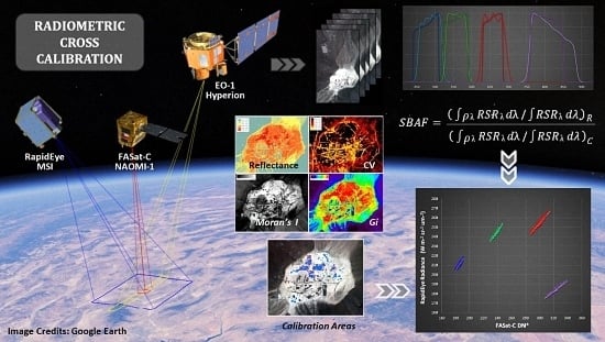
Radiometric Cross-Calibration of the Chilean Satellite FASat-C Using RapidEye and EO-1 Hyperion Data and a Simultaneous Nadir Overpass Approach

Abstract

The absolute radiometric calibration of a satellite sensor is the critical factor that ensures the usefulness of the acquired data for quantitative applications on remote sensing. This work presents the results of the first cross-calibration of the sensor on board the Sistema Satelital de Observación de la Tierra (SSOT) Chilean satellite or Air Force Satellite FASat-C. RapidEye-MSI was chosen as the reference sensor, and a simultaneous Nadir Overpass Approach (SNO) was applied. The biases caused by differences in the spectral responses of both instruments were compensated through an adjustment factor derived from EO-1 Hyperion data. Through this method, the variations affecting the radiometric response of New AstroSat Optical Modular Instrument (NAOMI-1), have been corrected based on collections over the Frenchman Flat calibration site. The results of a preliminary evaluation of the pre-flight and updated coefficients have shown a significant improvement in the accuracy of at-sensor radiances and TOA reflectances: an average agreement of 2.63% (RMSE) was achieved for the multispectral bands of both instruments. This research will provide a basis for the continuity of calibration and validation tasks of future Chilean space missions.

1. Introduction

There is common agreement among the remote sensing community that quantitative analysis and monitoring of the Earth’s surface processes require accurate and consistent measurements from satellite sensors, and this relies on absolute radiometric calibration [1,2,3,4,5]. This is especially valid when the information provided by a specific mission must be integrated with data from other platforms, either into models or multitemporal datasets [6,7,8].

The Sistema Satelital de Observación de la Tierra (SSOT), known as the FASat-C satellite, was launched on 16 December 2011, carrying the New AstroSat Optical Modular Instrument (NAOMI-1) [9,10]. FASat-C has been a successful Chilean satellite mission and has provided data for a wide range of applications in the fields of environment and forestry, mining and disaster management, among others [9,11,12]. Moreover, the launch of the FASat-D satellite, which gives continuity to the FASat-C mission, is under consideration; in this context, Cal/Val activities and the exploration of potential sites in Chile are required for the compatibility of the data from the sensors on-board both FASat satellites.

Every space platform is affected by degradation processes during its operational life [13,14], one of the effects being the variation of the radiometric response of the instruments. In the case of satellites without an On-Board Calibrator (OBC), such as FASat-C, any variation must be monitored and compensated relying on vicarious targets, such as desert sites [5].

In 2013, Mattar et al. [9] performed an in-flight absolute calibration activity for FASat-C in Santiago, Chile, in which the reliability of the pre-flight calibration coefficients was assessed. The objective of the present research is to update the radiometric calibration coefficients of the multispectral bands of NAOMI-1, through a cross-calibration using the simultaneous nadir overpass approach [5,15,16,17,18], based on the research of Teillet et al. [19,20]. RapidEye-MSI was the reference sensor against which FASat-C was calibrated, and EO-1 Hyperion provided data for the calculation of a Spectral Band Adjustment Factor (SBAF) [21].

This article is organized as follows: Section 2 presents a brief background on the absolute calibration of satellite sensors in general and the required compensation factors. Section 3 describes the study area and the satellite data acquisition. Section 4 provides the details of the method applied for the cross-calibration of FASat-C. Section 5 presents the obtained results and a preliminary evaluation of the pre-flight and updated calibration. Section 6 includes a discussion about the factors that have influenced the results, and in Section 7, the conclusions of the study and future remarks are outlined.

2. Background on the Calibration of Satellite Sensors

2.1. Absolute Radiometric Calibration and Approaches

After launch, a satellite starts to operate in an extremely harsh environment; consequently, a degradation process in all of the components begins. Conditions, such as exposure to mechanical stress, ultra-violet (UV) radiation, cosmic rays, energy generated during solar flares, charged particles trapped in radiation belts and outgassing, affect all optical and electronic devices of a platform [22,23,24,25]. These factors degrade the imaging instrument, modifying the radiometric response measured in the laboratory prior to launch and generating variations that must be periodically studied and compensated. This is mandatory when the collected data need to be used to derive biogeophysical parameters of different land covers and to quantitatively monitor our planet’s ecosystems [26,27,28,29,30].

The absolute radiometric calibration is defined as the process of quantifying the response of a sensor to known and controlled signal inputs [30,31]. The calibration plays a key role in the detection and monitoring capability of a satellite sensor [32], since the collected information that will be used (1) either to spectrally characterize a surface or (2) as an input to a model relies on how accurately the registered signal can be related to the respective incoming radiance. If the calibration parameters are not well known, any change in the response of the sensor could incorrectly be attributed to variations in the observed scene [33]. Hence, the success of any satellite mission and the feasibility of quantitative remote sensing applications are necessarily tied to Cal/Val activities [34].

The calibration parameters can be determined either directly, by an OBC device that provides a known signal to the sensor [35], or using indirect or vicarious methods that are totally independent from calibrations conducted in the laboratory or via OBC. Among the vicarious calibration methods, two categories can be differentiated, depending on the availability and usage of in situ measurements. On the one hand, the following approaches do require in situ measurements: reflectance-based [3,34,35,36], radiance-based [37] and irradiance-based approaches [38]. On the other hand, there are other approaches that only use remote measurements based on: (1) Rayleigh or molecular scattering over oligotrophic oceanic areas [39,40,41]; (2) deep convective clouds [42,43]; (3) Pseudo-Invariant Calibration Sites (PICS) [44,45]; (4) the surface of the Moon [46,47]; and (5) radiometrically well-characterized stellar sources [48,49,50].

Another widely-used alternative is cross-calibration, which consists of estimating the calibration coefficients of a sensor using as a reference another well-known instrument [19,20,51,52,53,54,55,56,57,58]. A cross-calibration can be applied when the OBC source is not available on the satellite [52,55,56,57,58], to proceed with a combined approach [51,56,59] or to tie data from different missions to a common radiometric scale [5,60].

2.2. Compensation Factors

The reduction of uncertainties in a cross-calibration procedure depends on the compensation of a series of variables, such as differences in illumination geometry, reflectance anisotropy effects and discrepancies between the Spectral Response Function (SRF) of the instruments, amongst others [19,21,61,62,63,64].

According to the cross-calibration approach proposed by Teillet et al. [19,20], two main compensations must be conducted. The first one is performed applying an illumination adjustment factor that includes the solar zenith angle at the time of acquisitions and the exo-atmospheric solar irradiance coefficients of both sensors. Since there is evidence that SRF is of critical significance, the second compensation is related to the spectral characteristics of the instruments. Two sensors that simultaneously observe the same land cover, at equivalent wavelengths, will offer different results, and a Spectral Band Adjustment Factor (SBAF), as proposed by Chander et al. [21], can be used to solve this source of mismatch.

Several studies have assessed the impact of the SRF differences on reflectance and spectral indices [2,17,21,61,62,63,64,65,66,67]; systematic biases of up to 30% in reflectance and 10% for vegetation indices have been reported, depending on the chosen sensors and their spectral bands. Data acquired by hyperspectral satellite and airborne sensors, such as EO-1 Hyperion, Scanning Imaging Absorption Spectrometer for Atmospheric Cartography (SCIAMACHY) and Airborne Prism Experiment (APEX), along with radiative transfer modeling, have been utilized to compensate existing differences.

A detailed study on the assessment of other sources of uncertainty and their influence on the radiometric cross-calibration can be found in Chander et al. [8].

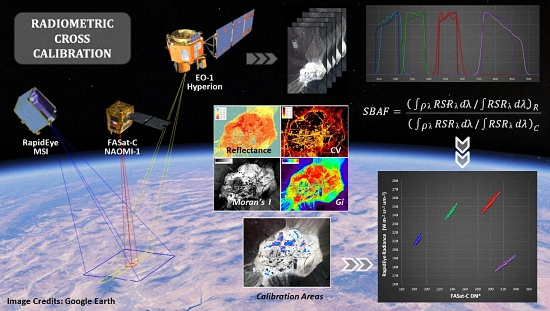
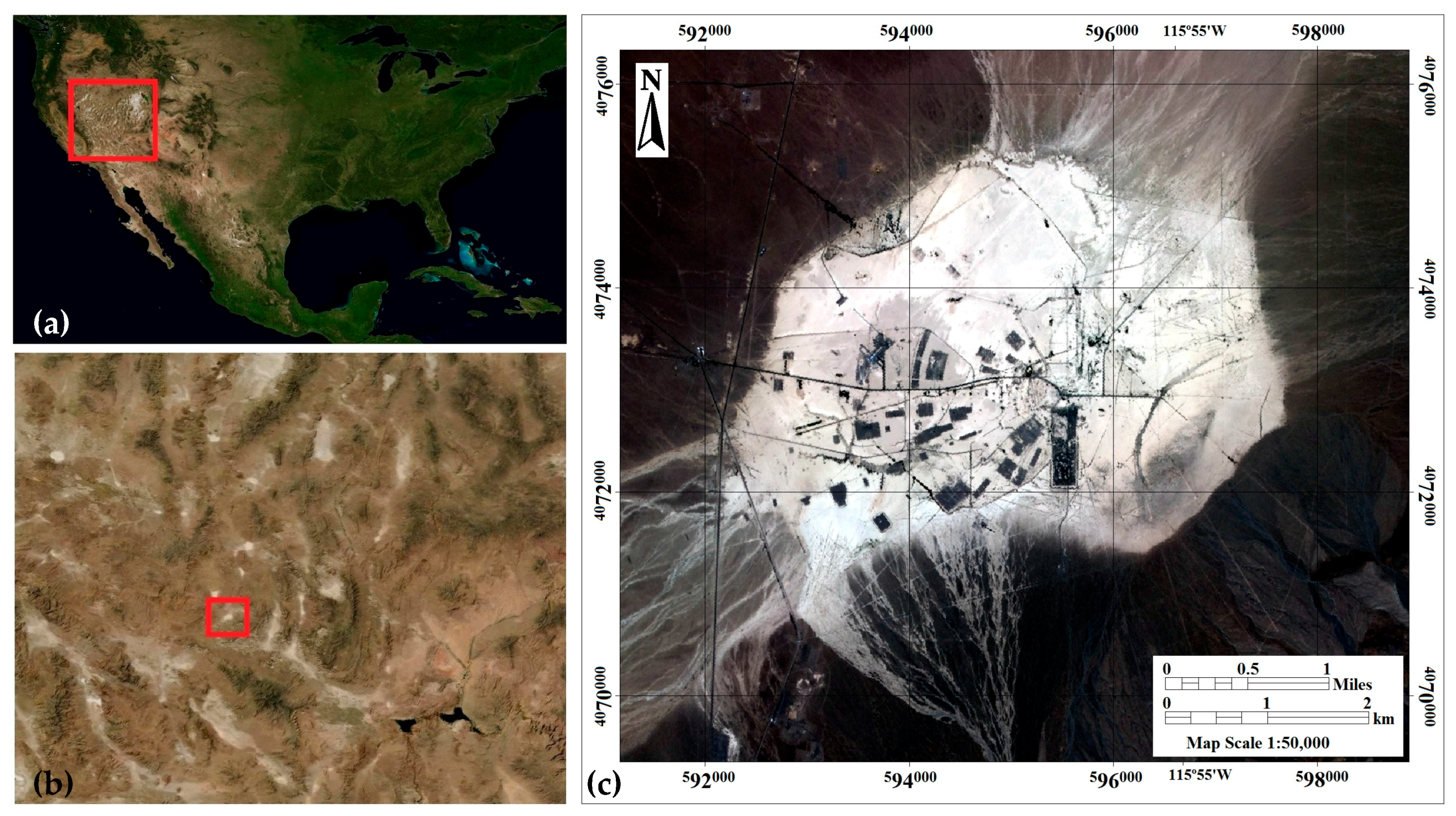
3. Study Area and Satellite Data

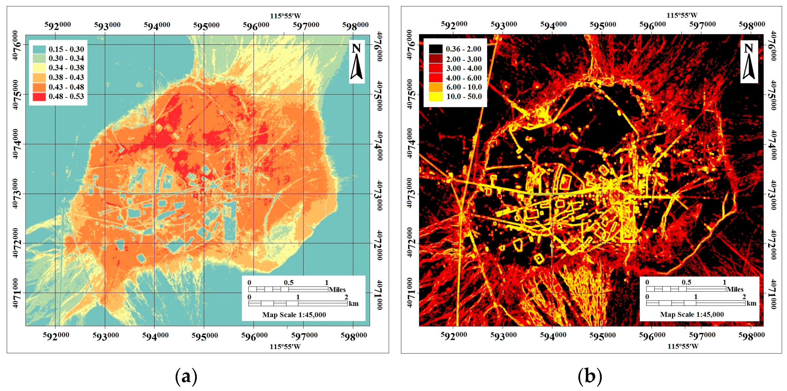
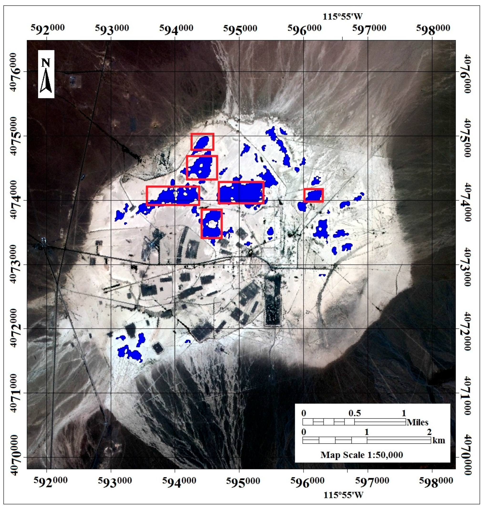
3.1. Frenchman Flat Calibration Site

The Frenchman Flat calibration site is located in Nevada, USA, in the transition zone of the Mohave and Great Basin deserts [68] (Figure 1). The area is a dry lake bed at 940 m.a.s.l.; formed of fine-textured sedimentary deposits, mainly sand, gravel, silt and clay [69]. The site fulfills many of the requisites stated by Thome [34] and Scott et al. [70] and belongs to the group of calibration sites endorsed by the Working Group on Calibration and Validation (WGCV) of CEOS [31,71]. The reflectance of the site is higher than 30% in the VIS/NIR domain, ensuring a high signal-to-noise ratio (SNR). It presents a high degree of spatial homogeneity over an area that allows the absolute calibration of sensors having a Ground Sampling Distance (GSD) smaller than 300 m [6,31]. Another characteristic of the area is its spectral uniformity, which contributes to minimizing the influence of SRF differences on the cross-calibration of satellite sensors [21,62,72].

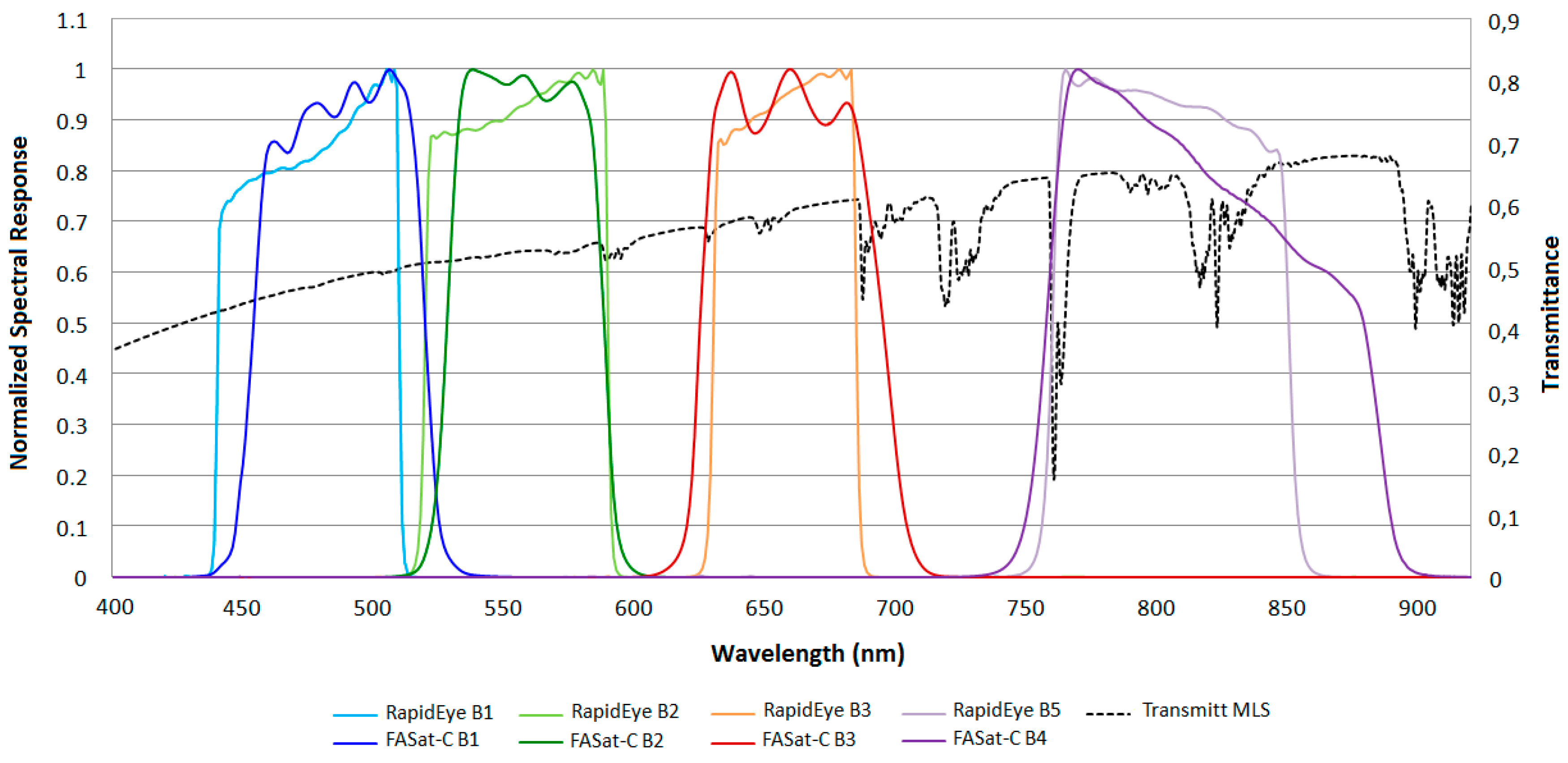
3.2. Overview of Sensors and Satellite Data

The NAOMI-1 sensor provides multispectral and panchromatic images with a periodicity of 37 days at-nadir conditions. Considering the satellite’s roll capability of ±30°, the revisit period is reduced to 3–5 days. The technical specifications of NAOMI-1 are reviewed in

Table 1. Technical specification of the MSI RapidEye and NAOMI-1 FASat-C sensors.

Specifications	RapidEye-MSI (RE4)	FASat-C NAOMI-1
Orbital height (km)	630	620
Nominal GSD at-nadir (m)	6.5	5.8
Dynamic range (bits)	12	10
Swath (km)	77	10
Descending node	11:00 a.m.	10:30 a.m.
Spectral Bands (nm)
Blue	440–510	455–520
Green	520–590	528–588
Red	630–685	625–695
NIR	760–850	758–881

, and more details can be found in Mattar et al. [9] and Aerial Photogrammetric Service (SAF) [10].

RapidEye is a five-satellite constellation launched on 29 August 2008, able to provide data on a daily basis at off-nadir conditions and every five days at-nadir [73]. Each satellite of the mission, named from RE1–RE5, carries identical MSI instruments. The requirements of the mission are radiometric stability over time and between spacecraft. The response between the same bands is within 5% over the whole mission, providing directly comparable images [74,75]. Since 2009, annual field campaigns have been conducted at Ivanpah Playa, Railroad Valley Playa (RVP) and Brookings calibration sites [76]. The Cal/Val activities have been performed by Blackbridge, in conjunction with the Universities of Arizona and South Dakota State. Since 2011, simultaneous collections for the whole constellation have been considered. The results of a validation performed over RVP indicated that, after the calibration updates of early 2014, the percentage differences between field measurements and MSI imagery were below 3% for the whole constellation (personal communication) [77]. In the case of RapidEye-4 (RE4), the sensor that acquired the data involved in the present work, the maximum differences were in the order of 1.25% [78]. More details about MSI are presented in Table 1, and a comparison of the relative spectral response (RSR) of both sensors is presented in Figure 2.

Data acquired by the EO-1 Hyperion Hyperspectral Imager (HSI), a pushbroom sensor of 198 calibrated bands of ~10 nm Full Width at Half Maximum (FWHM) in the range of 400–2500 nm [79], were used to obtain SBAF. The Hyperion spatial resolution is 30 m, and the dimensions of the scans are 7.5 km × 100 km.

On 25 July 2014, simultaneous acquisitions over Frenchman Flat were obtained by FASat-C and RapidEye (

Table 2. Satellite acquisitions over the Frenchman Flat calibration site.

36.8108° N; 115.9313° W	RapidEye (RE4)	FASat-C
UTC Time	19:22	18:51
Incidence Angle	3.760	1.237
Sun Azimuth Angle	158.437	138.372
Sun Elevation Angle	71.912	69.070
Satellite Azimuth Angle	279.570	100.084
Satellite View Angle	3.401	−1.127

). According to Cao et al. [15] and Teillet et al. [19,20], this approach helps minimize the uncertainties associated with differences in the atmospheric conditions and illumination geometry.

The FASat-C image was acquired by the Space Operations Group (GOE), and the respective Level 1A product was provided to the authors by SAF. More details about the data request can be found in SAF [10]. The RapidEye L1B imagery was provided as demo data by Blackbridge, to support this cross-calibration study. EO-1 Hyperion data of the study area in Hierarchical Data Format (HDF) were downloaded from the National Aeronautics Space Agency (NASA) Earth Explorer server [80]. The most recent cloud-free acquisitions were selected (

Table 3. EO-1 Hyperion acquisitions employed for SBAF estimation.

Date	5 October 2007	4 August 2008	12 January 2009	15 June 2009	25 February 2010	22 July 2010	7 February 2013
UTC Time	18:14:29	18:11:15	18:03:01	18:08:19	18:07:44	18:06:15	17:56:38
Sun Azimuth Angle	152.137	125.500	151.502	116.224	145.151	119.035	145.445
Sun Elevation Angle	44.722	60.636	26.370	65.377	37.620	61.920	30.766
Inclination Angle	98.10	98.09	98.20	98.10	98.19	98.08	98.12
Satellite View Angle	12.425	5.981	−9.094	0.432	−0.595	−3.364	6.603

).

4. Methods

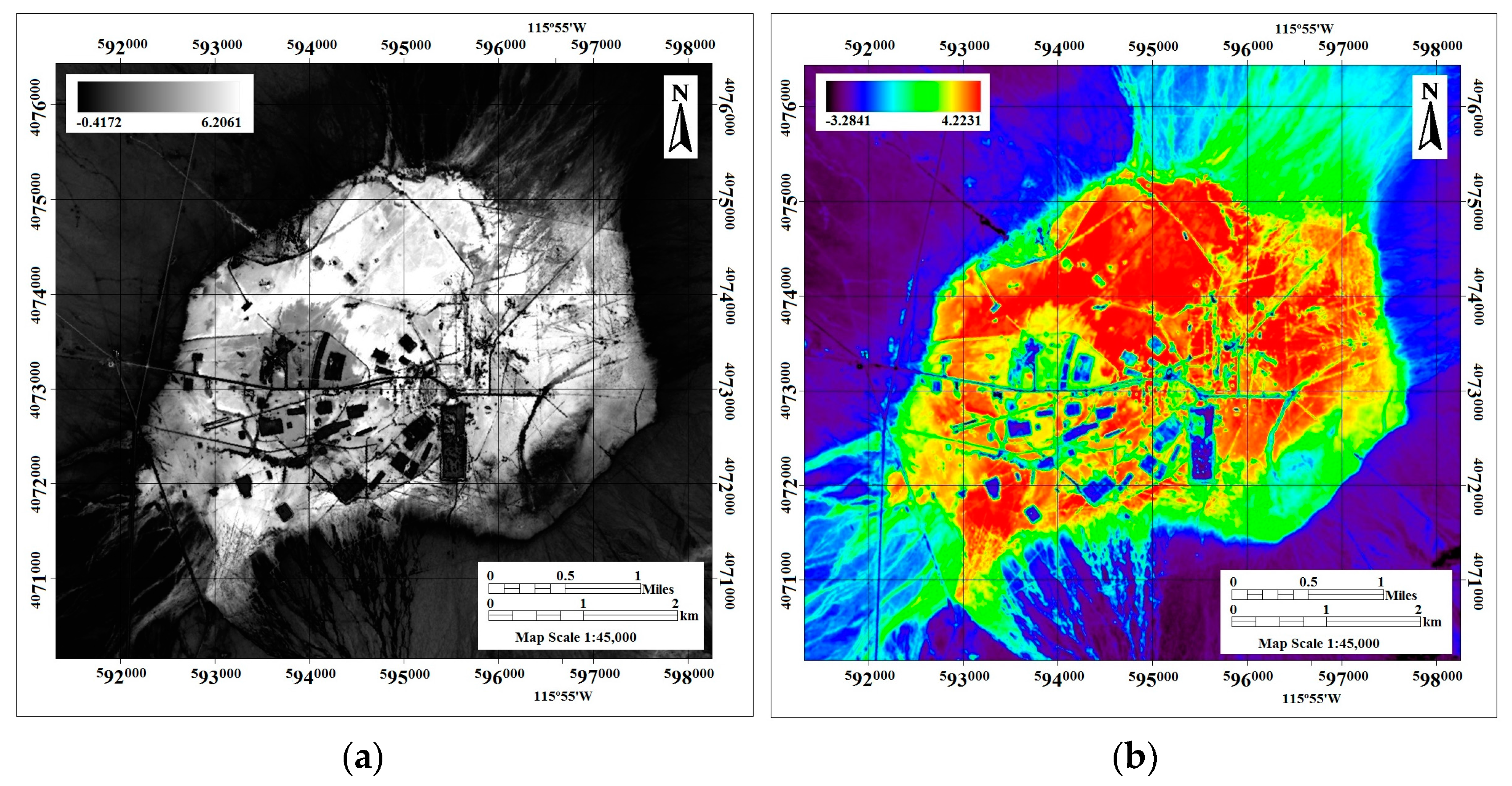
4.1. Spatial Autocorrelation and Uniformity Analysis

After the preprocessing stage, consisting of radiometric correction of the Level 1R Hyperion data and co-registration of the whole dataset to WGS84 UTM Zone 11 North system, the relative uniformity and spatial autocorrelation of the calibration site were examined. The Coefficient of Variation (CV) and Local Indicators of Spatial Association (LISA), specifically local indices of the Moran (I) [81] and the Getis Ord statistics (Gi) [82], were obtained for high spatial resolution data of Frenchman Flat. These indicators have been used by Cosnefroy et al. [44], Bannari et al. [83,84] and Odongo et al. [85] for the identification and characterization of suitable areas for the absolute calibration of satellite sensors.

The CV was derived for each band considering a 5 × 5-pixels window [84], and Gi and I were calculated under the Queen’s rule. The following thresholds were established to select the most homogeneous areas across the playa: CV ≤ 2%, Gi ≥ 3.2 and I ≥ 3.5. The threshold limits were empirically defined, testing different values of the above-mentioned indices, as follows: (1) selecting and applying the values for CV, I and Gi; (2) vectorizing the obtained images; (3) intersecting the layers corresponding to each index; and (4) visually evaluating the extension of the resulting polygons, according to the information provided in Polder et al. [71]. The previous steps were repeated until areas with the characteristics of the specific LED-Based Spectral Surface Monitoring (LSpec) calibration site were delineated. In order to reduce the influence of registration errors, caused by differences in spatial resolution [58,72], these criteria were applied for the identification of the most homogeneous areas, from which the samples for the cross-calibration of FASat-C were extracted.

4.2. Sample Extraction

At uniform and highly-reflective clusters, resulting from thresholding and the intersection of the layers previously generated, 130 samples of 5 × 5 pixels were collected from FASat-C and RapidEye imagery for cross-calibration. Additionally, for a preliminary evaluation of the results, 300 samples were randomly collected across the whole common area of both acquisitions, although it was not possible to maintain the same pattern, due to the lack of some land covers in the neighborhood of the site. Water bodies or dense vegetation with sufficient extension, according to the GSD of both sensors, were not available in Frenchman Flat; thus, the few vegetation samples identified cover areas of just 3 × 3 pixels. Regarding the outlier detection, for both calibration and evaluation samples, the FASat-C digital numbers (DN) were plotted against RapidEye radiances, with outliers being considered the measurements more than two standard deviations (2σ) away from the best-fit line.

4.3. E₀ Calculation for FASat-C

The exo-atmospheric spectral solar irradiance coefficients (E₀) were employed to calculate the compensation factors and to derive FASat-C TOA reflectances. In order to avoid introducing additional systematic errors, hence to ensure a consistent calculation of compensation factors and TOA reflectances for all involved sensors, the same solar irradiance model was employed. The reason is that depending on the solar model, relative differences of up to 2% will arise [9,51,86], affecting the Ai factor and cross-calibration results. E₀ values were estimated with Equation (1), using the solar irradiance model of Thuillier [87], as recommended by CEOS [31]. Sampling intervals of the solar model were linearly interpolated to the RSRs.

$$E_0={\displaystyle \int }{S}_{\lambda }RS{R}_{\lambda } d\lambda /{\displaystyle \int }RS{R}_{\lambda } d\lambda$$

(1)

where S_λ is the solar irradiance model of Thuillier [87] expressed in W·m⁻²·μm⁻¹ and RSR_λ is the relative spectral response of the band.

4.4. Compensation Factors

In the overlap area covered by the 3 sensors, 15 samples of 5 × 5 pixels each were extracted from every scan of Hyperion, and the time-averaged TOA reflectances were calculated to derive the SBAF (2), as presented by Chander et al. [21]. The Hyperion TOA reflectance was resampled to match the 1-nm sampling interval of the RSR of both sensors. Simulated TOA reflectance for both sensors were obtained by integrating the RSR and Hyperion spectral signatures, weighted by the RSR. The convolution of the numerator corresponds to the simulated TOA reflectance of the reference sensor and the denominator to the sensor to be calibrated; the ratio being an indicator of the difference arising from the RSR mismatch for a given band and target [21,62].

$$SBAF=\frac{{\left(\int {\rho }_{\lambda }RS{R}_{\lambda } d\lambda /\int RS{R}_{\lambda } d\lambda \right)}_R}{{\left(\int {\rho }_{\lambda }RS{R}_{\lambda } d\lambda /\int RS{R}_{\lambda } d\lambda \right)}_F}$$

(2)

$${\rho }_F^{ *}= {\rho }_F^{ } SBAF$$

(3)

where ρ_λ is the hyperspectral TOA reflectance of a sample; RSR_λ is the relative spectral response of a sensor; R is RapidEye MSI, the reference sensor; F is FASat-C NAOMI-1, the sensor to be calibrated against R; ρ_F * is the reflectance of the sensor F, compensated by the RSR difference effects. The SBAF can be applied to DNs or to at-sensor radiances of F, as well. Two factors were obtained to be applied differentially to calibration (Cal) and evaluation samples (Eva): SBAF_Cal and SBAF_Eva, respectively. SBAF_Cal was derived with 5 samples collected at the defined homogeneous zones (Figure 3) and SBAF_Eva using 10 samples collected over the whole FASat-C scene, covering the range of reflectances available in the study area.

For the compensation of illumination differences, an adjustment factor was calculated, following Teillet et al. [19,20]. This factor was multiplied by SBAF, and the resulting product was incorporated into a final factor named Ai (Equation (4)).

$$Ai=SBAF{\left(E_{0}cos\theta \right)}_R/{\left(E_{0}cos\theta \right)}_{F }$$

(4)

where E₀ are the exo-atmospheric solar irradiance coefficients of the respective sensor (R and F) obtained with Equation (1), expressed in W·m⁻²·μm⁻¹; θ are the zenith angles corresponding to the data acquisition of R and F.

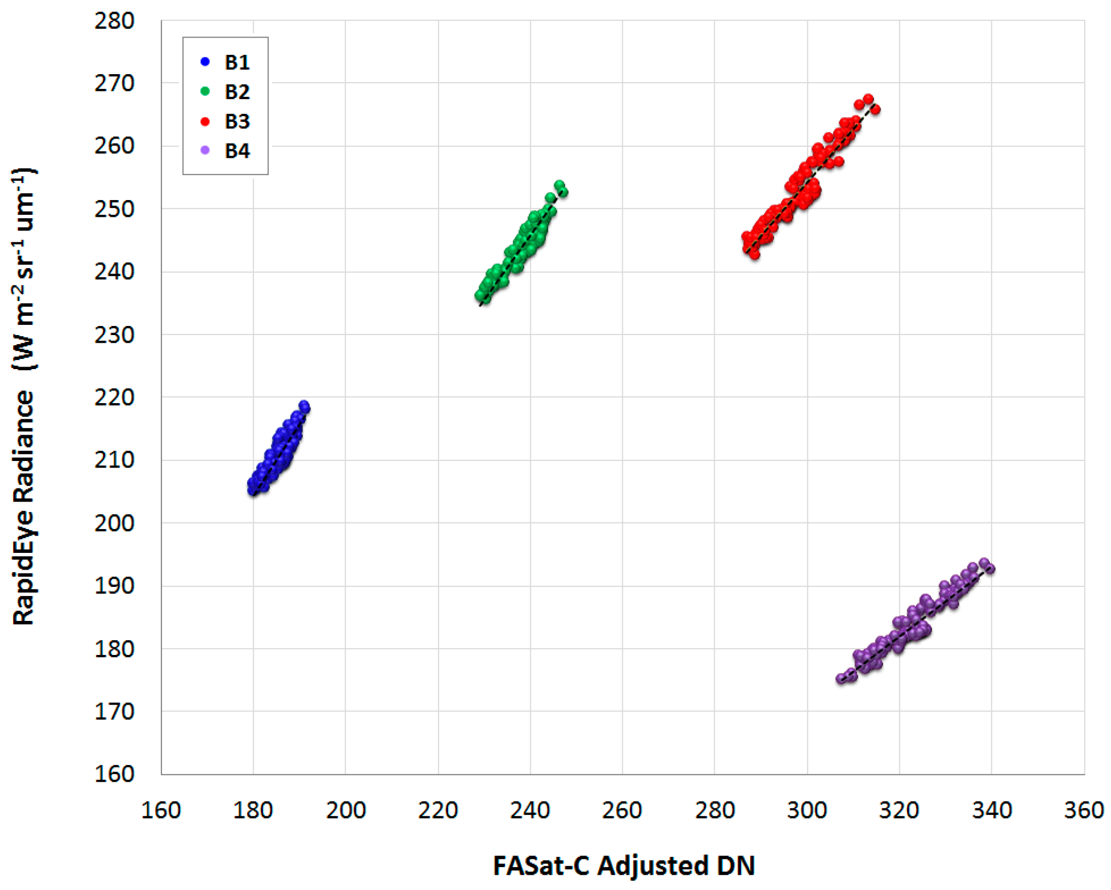
4.5. Cross-Calibration of FASat-C NAOMI-1

The average FASat-C DN per sample were adjusted by multiplying the Ai factor Equation (4). For both sensors, the offset values are periodically estimated on a pixel basis during the relative radiometric calibration process, performed over dark oceanic areas, and are subtracted at the Level 1A/1B product generation [10,74]. The RapidEye radiances were obtained applying the radiometric scale factor given in the metadata file (9.999999776483 × 10⁻³ W·m⁻²·sr⁻¹·μm⁻¹) to all bands, as follows Equation (5):

$$L_R=G_R D{N}_R$$

(5)

The absolute radiometric calibration coefficients of NAOMI-1 bands were obtained through a linear fit, considering Equations (6)–(8):

$$L_F=D{N}_F G{ }_F^{-1}$$

(6)

$$\frac{D{N}_R}{D{N}_F}=\frac{{\rho }_R {\left(E_{0}cos\theta \right)}_R}{{\rho }_F G_R G_F{\left(E_{0}cos\theta \right)}_F}$$

(7)

$$D{N}_F^{ *}=Ai D{N}_F= L_{R }{G}_F$$

(8)

where L_R and L_F are the at-sensor radiance of the F and R sensors, expressed in W·m⁻²·sr⁻¹·μm⁻¹; G_R and G_F are the gains of R and F, expressed in W·m⁻²·sr⁻¹·μm⁻¹; DN_R and DN_F are the digital numbers of R and F; ρ_R and ρ_F are TOA reflectances of F and R; DN_F* is the adjusted DN of the sensor to be calibrated against the reference sensor. In Equation (7), the term ρ_R/ρ_F is replaced by the SBAF and, in conjunction with (E₀ cosθ)_R/(E₀ cosθ)_F, constitutes the final compensation factor Ai, previously obtained using Equation (4).

5. Results

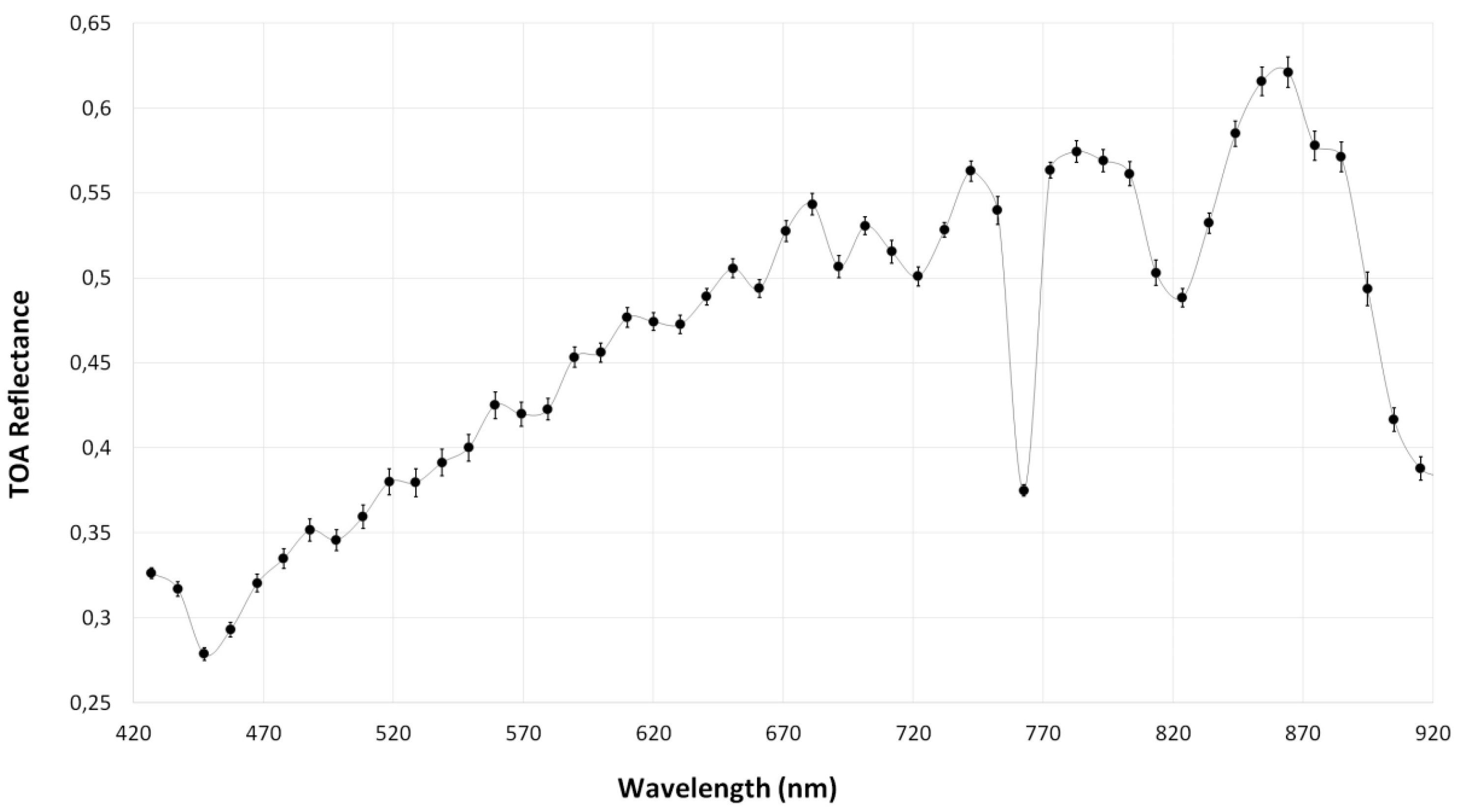
5.1. Spatial Analysis of the Calibration Site

As spatial homogeneity is one of the most important factors for the assessment of calibration sites [70,72,83,84,85], the calculation of Moran’s I, the Getis Ord Gi, CV and TOA reflectance were essential for the selection of specific areas in the Frenchman Flat site, for the calibration (Figure 4 and Figure 5).

Particularly, I and Gi provided valuable information regarding the spatial patterns that are undetectable to CV or to global indicators of spatial dependence [83,84,85]. It must be mentioned that, as a result of the applied thresholding criteria, about 85% of the samples used for the estimation of FASat-C gains presented a CV lower than 1%. This has ensured that the most homogeneous and spatially-autocorrelated areas of Frenchman Flat were used for the cross-calibration of FASat-C (Figure 6). This is in line with the research of Feng et al. [56] and Gao et al. [58], who selected regions of interest located in areas with such relative variability for Cal/Val activities of the Chinese High Resolution Imaging Satellite GaoFen-1.

After excluding outliers, the following number of homogeneous samples were used for the calibration: 127 for the blue (B1), 125 for the green (B2), 128 for the red (B3) and 129 for the NIR (B4) bands, respectively. Since the amount of photons reaching the sensor and their energy vary according to wavelength, each band was considered as an independent experiment. The FASat-C adjusted DNs and the RapidEye radiances exhibited a linear behavior and a high degree of correlation.

5.2. E₀ and Compensation Factors

The published E₀ values for RapidEye are 2003, 1824, 1571 and 1117 for the blue, green, red and NIR bands, respectively [88]. In

Table 4. Parameters and compensation factors estimated for the cross-calibration of FASat-C.

Band	E0	Illumination	SBAFCal	St Dv SBAFCal	AiCal	SBAFEva	St Dv SBAFEva	AiEva
B1	1975.85	1.03172	0.96608	0.0009	0.99672	0.97882	0.0115	1.00987
B2	1825.06	1.01715	0.99860	0.0001	1.01573	0.99971	0.0011	1.01686
B3	1536.95	1.02042	1.00583	0.0003	1.02637	1.00516	0.0010	1.02569
B4	1027.58	1.10630	0.97358	0.0016	1.07707	0.97219	0.0023	1.07553

, the exo-atmospheric irradiance coefficients for FASat-C (W·m⁻²·sr⁻¹·μm⁻¹) and the compensation factors are provided. For consistency, E₀ values of RapidEye were obtained and compared against the given coefficients, and differences within the range 0.4–4.8 W·m⁻²·μm⁻¹ were obtained, where the maximum discrepancy corresponds to the NIR band.

According to SBAF values, for all FASat-C bands, but B3, values lower than unity show a higher amount of in-band reflectance in comparison to RapidEye, either for Cal or Eva compensation factors, the cause being the shape of the FASat-C spectral responses and the features of the Hyperion TOA reflectance spectra employed to derive the SBAF values. Chander et al. [21] mentioned that SBAF is more sensitive to variations in slope or spikes present in hyperspectral TOA reflectance spectra rather than to magnitude disparities. This point may explain the low standard deviation values, especially for SBAF_Cal. The NIR band presents higher variability due to the presence of water vapor absorption features [8,21,54,61]. Nonetheless, for SBAF_Cal and SBAF_Eva, this variability may also reveal a temporal variation in TOA reflectance due to the differences in observation, illumination or atmospheric conditions. Besides, in the case of SBAF_Eva, the differences could possibly be related to a seasonal component (e.g., phenology of vegetation and soil moisture variation).

5.3. Radiometric Cross-Calibration

As offsets have been subtracted during the generation of the radiometrically-corrected products, the results obtained through linear fits forced to the zero intercept, I₀, referred to hereinafter as the result of the cross-calibration, were chosen. Just as a reference, the free-intercept (F_i) results are included; however, the R² coefficient does not greatly differ from the I₀ outcomes, and a similar amount of variability is explained by the linear fit, except for B1. A scatterplot of RapidEye radiances and FASat-C adjusted DN samples and cross-calibration results are provided in Figure 7 and

Table 5. FASat-C radiometric calibration parameters estimated over Frenchman Flat.

Band	n	Free Intercept (Fi)			Zero Intercept (I0)		Pre-Flight Calibration (Pre-F)
		Gain	Offset	R2	Gain	R2	Gain Pre-F−1	Δ Gain (I0—Pre-F−1)
B1	127	0.9941	26.266	0.8418	1.1357	0.8248	1.0708	5.71%
B2	125	0.9691	12.787	0.9284	1.0230	0.9255	0.9867	3.55%
B3	128	0.8631	−4.605	0.9391	0.8476	0.9388	0.8239	2.78%
B4	129	0.5741	−1.696	0.9260	0.5688	0.9259	0.63068	−10.88%

, respectively.

The degree of dispersion around the best-fit line is considered to be mainly a consequence of the angular anisotropic effects of reflectance; this factor has neither been studied nor corrected for, since it is out of the scope of this work. The absolute radiometric parameters estimated during pre-flight calibration are provided in Table 5. Relative differences between Pre-Flight (Pre-F) and I₀ estimated gains are detailed, as well (Δ_Gain).

Considering the equation of FASat-C radiance, relative percentage differences have been calculated using the inverse value of the respective per-band gains. Absolute gains of Bands 1, 2 and 3 have shown an increase of 5.71%, 3.55% and 2.78% in radiance units per DN, respectively, while B4 presents a decrease of −10.88%.

To assess the influence of the size of the calibration sample on the estimated gains, 32 samples of 10 × 10 pixels each were collected on the same regions that were catalogued as uniform and highly correlated. An average relative difference of 0.16% with respect to the gains estimated with the 5 × 5-pixels samples was obtained. These gains were applied to the evaluation samples, causing an average difference of 0.04% in the RMSE values of absolute errors.

A study about the dependence on sample size (i.e., 5 × 5 pixels vs. 10 × 10 pixels) of the per-band coefficients of the I₀ models showed an average decrease of 25.2% in the coefficients for all bands; reducing the goodness of fit of the linear models when the largest sample size is chosen. However, it must be emphasized that the relative differences between both I₀ gain sets have low impact on the calculated radiances/reflectances. These results demonstrate the importance of calibrating satellite sensors with a CEOS-WGCV endorsed site and the potential of LISA to define specific calibration regions, as shown in Bannari et al. [83,84] and Odongo et al. [85].

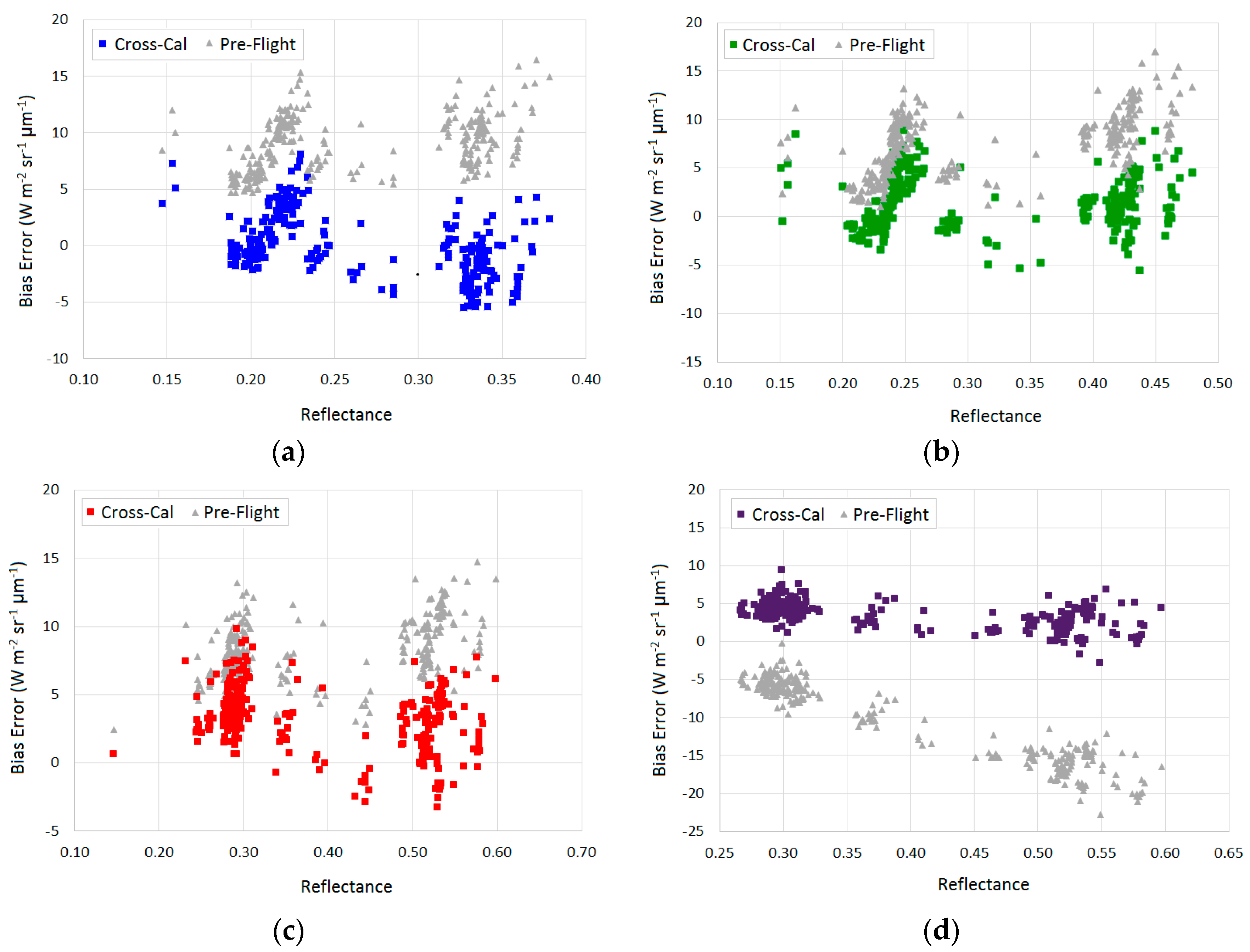
5.4. Preliminary Evaluation Results

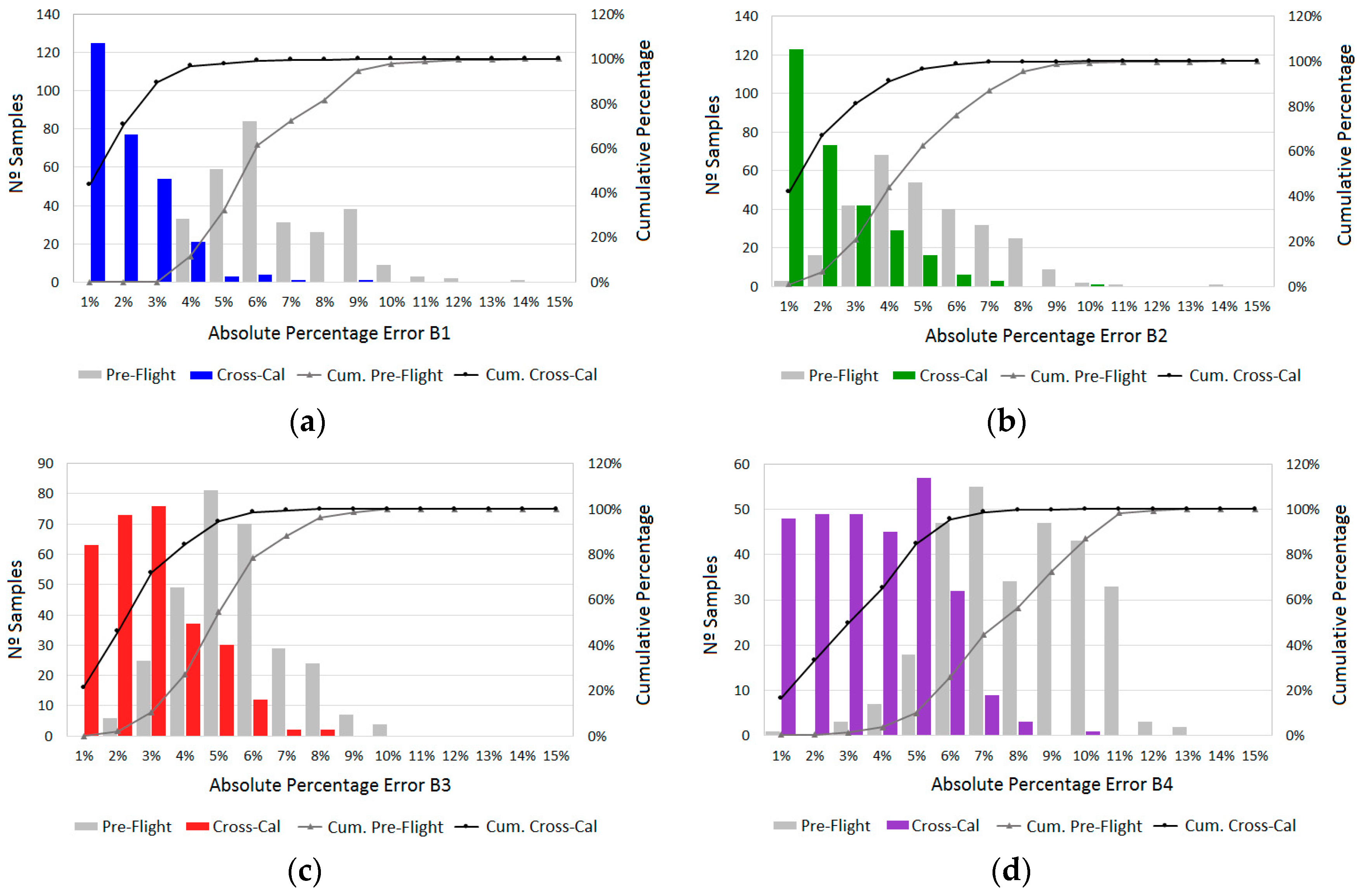
5.4.1. Per-Band Bias Errors

For the evaluation of both sets of calibration coefficients, the number of remaining samples after outlier filtering was 286, 293, 295 and 293, for B1, B2, B3 and B4, respectively. This evaluation is just a preliminary exploration of the results obtained applying coefficients I₀ and Pre-F, mainly due to the fact that there is no land cover diversity in the area covered by both sensors. Hence, a validation must be considered over heterogeneous zones with the presence of different types of vegetation, soils, etc., in the form of large uniform patches. Under these circumstances, the evaluation of the estimated gains over a broader range of reflectances for each FASat-C band would be feasible.

In order to allow the comparison of both calibration parameters sets (Pre-F and I₀), per-sample bias errors were calculated with respect to RapidEye radiances and reflectances.

Table 6. MBE for FASat-C at-sensor radiances (W·m⁻²·sr⁻¹·μm⁻¹) and TOA reflectances of FASat-C with respect to RapidEye.

Band	Cal	Radiance					Reflectance
		MBE	St Dv	Median	Max	Min	MBE	St Dv	Median	Max	Min
B1	Pre-F	9.03	2.43	9.26	16.48	4.70	0.015	0.004	0.016	0.028	0.008
	I0	0.17	2.79	−0.29	8.11	−5.45	0.000	0.005	0.000	0.014	−0.009
B2	Pre-F	7.57	3.22	8.06	17.10	1.12	0.014	0.006	0.015	0.032	0.002
	I0	1.67	2.82	1.33	8.95	−5.48	0.003	0.005	0.002	0.017	−0.010
B3	Pre-F	8.17	2.22	7.91	14.73	2.45	0.018	0.005	0.018	0.033	0.005
	I0	3.36	2.27	3.51	9.80	−3.30	0.007	0.005	0.008	0.022	−0.007
B4	Pre-F	−10.37	5.28	−8.02	−0.23	−22.76	−0.032	0.016	−0.024	−0.001	−0.069
	I0	3.40	1.75	3.62	9.41	−2.88	0.010	0.005	0.011	0.029	−0.009

summarizes the main descriptive statistics for all FASat-C bands, such as Mean Bias Error (MBE), among others. The mean bias error of the evaluation samples was obtained as follows:

$$\text{MBE}= \frac{1}{n}{\displaystyle \sum }_{i=1}^n{\left(R-F\right)}_i$$

(9)

where n is the number of evaluation samples; R and F are the magnitudes derived from the common samples collected by RapidEye and FASat-C, respectively (radiance or reflectance).

When compared to RapidEye, the use of Pre-F gains led to an underestimation of at-sensor radiances for B1, B2 and B3, and an overestimation for B4. The cross-calibration produced less biased results, and the best agreements were obtained for B1 and B2. The cross-calibration reduced the B1 MBE from 9.03 down to 0.17 W·m⁻²·sr⁻¹·μm⁻¹ and the B2 MBE from 7.573 down to 1.67 W·m⁻²·sr⁻¹·μm⁻¹. For B3, the mean bias error decreased from 8.17 down to 3.36 W·m⁻²·sr⁻¹·μm⁻¹, while for B4, it changed from −10.37–3.4 W·m⁻²·sr⁻¹·μm⁻¹. In spite of the high variability observed in the sample, particularly for B1 and B2, for which the standard deviations are higher than MBE, a considerable decrease in the magnitude of MBE and maximum bias errors was achieved once I₀ gains are utilized.

In Figure 8, the bias error per sample is shown as a function of TOA reflectance, either for pre-flight or for cross-calibration. For B1 (Figure 8a), after cross-calibration, the range of bias errors shifted from 4.7–16.5 W·m⁻²·sr⁻¹·μm⁻¹ to −5.45–8.1 W·m⁻²·sr⁻¹·μm⁻¹, corresponding the highest bias errors to samples of ~0.15 and ~0.22 reflectance units. Radiances equivalent to reflectances higher than 0.25 are mainly overestimated; nevertheless, the biases for all samples have been substantially reduced.

For B2 (Figure 8b), after cross-calibration, underestimation has lessened if compared to the results obtained after applying the Pre-F gain. With Pre-F gain, the bias errors were in the range of 1.12–17.1 W·m⁻²·sr⁻¹·μm⁻¹; after applying the I₀ gain, the range of bias error changed to −5.48–8.95 W·m⁻²·sr⁻¹·μm⁻¹, meaning that the improvement is more noticeable for higher reflectance samples. The range has been reduced, along with the MBE and dispersion, which shows the good performance of the updated parameter.

In the case of B3 (Figure 8c), the radiances are underestimated using both Pre-F and I₀ gains. Nevertheless, a reduced percentage of the sample, concentrated between 0.45 and 0.6 of reflectance, presents overestimation after cross-calibration. Using Pre-F gains, the bias errors were in the range from 14.7–2.45 W·m⁻²·sr⁻¹·μm⁻¹; once I₀ gain was used, the values were in the range from −3.30–9.78 W·m⁻²·sr⁻¹·μm⁻¹. For this band, the decrease in MBE can be considered as a clear improvement, particularly at higher reflectances.

For B4 (Figure 8d), where noticeable differences existed among low and high reflectances before the application of the I₀ coefficients, overestimation increased with reflectance, mainly at reflectances higher than 0.5. Before cross-calibration, the bias ranged from −22.76–−0.23 W·m⁻²·sr⁻¹·μm⁻¹, which after the procedure was significantly reduced to the interval from −2.88–9.4 W·m⁻²·sr⁻¹·μm⁻¹. Although the bias was not completely removed, it considerably diminished after the cross-calibration against RapidEye.

5.4.2. Per-Band Absolute Error

The Mean Absolute Percentage Error (MAPE), the Root Mean Square Error (RMSE) of absolute percentage errors and other statistics of Pre-F and I₀ calibration parameter sets are presented in

Table 7. Absolute errors for FASat-C at-sensor radiances and TOA reflectances with respect to RapidEye.

Band	Calibration	RMSE	MAPE	St Dv	Min.	1st Quartile	Median	3rd Quartile	Max.
B1	Pre-F	6.27%	6.01%	1.81%	3.03%	4.80%	5.53%	7.35%	13.36%
	I0	1.94%	1.51%	1.23%	0.00%	0.56%	1.20%	2.15%	8.12%
B2	Pre-F	5.00%	4.61%	1.93%	0.79%	3.29%	4.26%	5.88%	13.10%
	I0	2.28%	1.71%	1.52%	0.01%	0.53%	1.23%	2.53%	9.90%
B3	Pre-F	5.18%	4.93%	1.59%	1.40%	3.90%	4.86%	5.79%	9.98%
	I0	2.75%	2.31%	1.50%	0.00%	1.20%	2.14%	3.09%	7.40%
B4	Pre-F	7.80%	7.52%	2.08%	0.24%	5.97%	7.50%	9.25%	12.66%
	I0	3.56%	3.05%	1.84%	0.00%	1.53%	3.04%	4.43%	9.60%

. The RMSE and MAPE, with respect to RapidEye, were obtained using the following expressions (Equations (10) and (11)):

$$\text{RMSE}= \sqrt{\frac{1}{n} {\displaystyle \sum }_{i=1}^n{\left(R_i-F_i\right)}^2}$$

(10)

$$\text{MAPE}= \frac{1}{n}{\displaystyle \sum }_{i=1}^n\left|\frac{R_i-F_i}{R_i}\right|\times 100$$

(11)

where n is the number of evaluation samples; R and F are the magnitudes derived from the common samples collected by RapidEye and FASat-C, respectively (radiance or reflectance).

Considering the skewness of the distribution of the APE of the I₀ samples (Figure 9), the first and third quartile values are also provided. As seen, after cross-calibration, the shape of the distribution of all bands has changed, with the samples being concentrated at the lower absolute errors, especially for B1 and B2. For B3, the trend is similar to B1 and B2, in the sense that the distribution of the absolute errors is left-skewed; however, absolute errors are concentrated below 3%, and not below 2%, as in the case of B1 and B2. In the particular case of B4, the distribution turns into a more uniform one.

Overall, once the updated coefficients are applied, the level of dispersion in the sample was reduced by 32%, 21%, 6% and 12% for B1, B2, B3 and B4, respectively.

For B1, the MAPE decreased from 6.01% down to 1.51% and the RMSE from 6.27% down to 1.94%; besides the median value of 1.2% must be observed in the case of I₀, since it would be more representative. In addition, the maximum error diminished from 13.4% down to 8.1%. According to B1 histograms (Figure 9a), using Pre-F gains, just 32% of the sample presented an absolute error of up to 5%, while 66% of the sample had absolute errors in the range 5%–10%. After the cross-calibration, 71% of the samples have errors of up to 2%; 27% are in the range 2%–5%; and just 2% of the sample present errors higher than 5%.

Results for B2 indicate that RMSE decreased from 5% down to 2.28% after cross-calibration, and MAPE dropped from 4.61% down to 1.71%. Besides, the maximum error diminished from 13.1% down to 9.9%, and the median value of the errors moved from 4.26% down to 1.23%. Prior to the calibration (Figure 9b), 62.5% of the sample had an error of up to 5% and 36.9% an error of up to 10%. Just 0.7% of the sample presented absolute errors higher than 10%. After cross-calibration, 66.9% of the sample presents errors of up to 2%; 29.7% of the sample has errors in the range 2%–5%; and just 2.1% has absolute errors larger than 5%.

For B3, the RMSE decreased from 5.18% down to 2.75% and MAPE from 4.93% down to 2.31%, while the median value of errors is 2.14%. The maximum error lessened from 9.98% down to 7.4% after cross-calibration. The frequency distribution of absolute errors using Pre-F calibration (Figure 9c) indicates that 54.6% of the samples present an error of up to 5%, and 45.4% of the sample is in the range between 5% and 10%. Once the radiometric calibration parameters have been updated, 46.1% of the sample has a maximum absolute error of 2%; 48.5% is between 2% and 5%; and just 5.4% of the samples is in the order of 5%–10%.

Lastly, for B4, the RMSE dropped from 7.8% down to 3.56%, MAPE from 7.52% down to 3.05%, and the maximum error diminished from 12.66% down to 9.6%. The median value of absolute errors changed from 7.5% down to 3.04%, once I₀ coefficients are applied to the DN samples. In relation to the distribution of errors (Figure 9d), prior to the B4 cross-calibration, 9.9% of the sample presented absolute errors of up to 5%; 77.1% was in the range 5%–10%; and 13% presented errors equal to or higher than 10%. The results obtained using the I₀ gain revealed that 33.1% of the sample contained errors of up to 2%; 51.5% has errors in the range of 2%–5%; and 15.4% has errors of the order of 5%–10%.

6. Discussion

Though the preliminary evaluation results indicate that the absolute errors of FASat-C with respect to RapidEye radiances and reflectances have been reduced, if the obtained values are compared to the errors prior to the cross-calibration, a validation process that includes cross-validation and in situ measurements should be performed over heterogeneous areas. This task will allow the evaluation of the new set of calibration coefficients over low reflectance targets, which were not represented in the sample due to the characteristics of the site.

According to Thome [34] and Scott et al. [70], low reflectances present a reduced SNR due to the increasing contribution of aerosols to at-sensor radiance. In relation to that topic, when assessing the uncertainty of an in-flight calibration, Chen et al. [89] found that for low-reflectance surfaces, uncertainties were higher than for more reflective targets, suggesting that the quality of remotely sensed data of darker areas should be carefully studied. Furthermore, considering all of the previous factors and what has been analyzed by Chander et al. [8], it must be added that most of the samples characterized by higher errors correspond to targets that are more sensitive to misregistration.

In the present work, BRDF (Bi-directional Reflectance Distribution Function) effects have not been corrected; it is therefore not unlikely that some of the high absolute errors are a consequence of the anisotropic behavior of reflectance. Moreover, according to Gürbüz et al. [6] and CEOS [31], the calibration site presents some debris from weapon tests; this can be another possible factor influencing the response of some validation samples at the sub-pixel level.

As atmospheric path radiance, diffuse radiance and related adjacency effects have not been removed during the cross-calibration process, some influence on the results can also be expected. In addition, areas from which evaluation samples were collected neither exhibit the lowest CV nor the highest degree of spatial autocorrelation; therefore, as stated by Hamm et al. [72], the adjacency effects would not be narrowed. This point may explain to some extent the higher standard deviations of MBE after cross-calibration, particularly for B1 and B2.

Another important issue to consider is the fact that the discrepancies of FASat-C B3 and B4, with respect to RapidEye, are larger than the ones existing for B1 and B2; this can be explained by the differences in the shape and magnitude of the SRF at the wavelengths where absorption features are located. The O₂ absorption feature at 630 nm is in the limit of the FWHM of RapidEye’s B3, although encompassed by B3 of FASat-C. At this specific wavelength, the responses of the two sensors differ by ~50%. The next O₂ feature at 690 nm is by-passed by the RapidEye SRF, but not by FASat-C B3. In the case of the NIR band, the water vapor absorption feature at 760 nm is located where the difference in the RSR of the sensors is ~25%. Besides, a H₂O feature at 820 nm is over an area of the spectrum in which the RSR of FASat-C differs by 17%, in relative terms.

In Figure 2, the RSR of both sensors and a MODTRAN (MODerate resolution atmospheric TRANsmission) [90] simulation of the transmittance for the mid-latitude summer atmosphere model are shown. The absorption features of the different atmospheric constituents can be observed. The transmittance presents a flat behavior within B1 and B2, while absorption features are noticeable for B3 and B4; thus, an influence of the overall shape of the RSR can be expected in this case.

In accordance with Chander et al. [21], the existence of other atmospheric features, non-detectable for the Hyperion ~10-nm spectral resolution, affects the SBAF and the degree of agreement between Rapid and FASat-C B3 and B4. In their research, the degree of agreement between the adjusted TOA reflectances of MODerate Resolution Imaging Spectroradiometer (MODIS) and Enhanced Thematic Mapper Plus (ETM+) increased by 1% once SCIAMACHY-based SBAFs were applied. Differences in the range of −3.01%–5.18% were reported between Hyperion-based and SCIAMACHY-based SBAFs, as well. In that case, the reported improvement was not only due to the 1-nm spectral resolution of SCIAMACHY, but also because of differences in the overall spectral shape of the reflectances measured by both sensors.

The results of the preliminary evaluation of the cross-calibration of FASat-C are affected by the lack of knowledge of SBAF over some targets, since differences in GSD do restrict the evaluation, at least over Frenchman Flat. As a result, the TOA reflectance of some targets cannot be properly characterized by the Hyperion 30-m GSD, which did not allow the estimation of SBAF over those areas. The averaged factors applied for the evaluation process could be a possible cause of the higher biases and absolute errors, mainly for lower reflectance targets that do not present Lambertian behavior. In that sense, the results presented in this work suggest that per-coverage SBAF calculations are required for validation purposes; then, for future validation activities, this point should be considered in order to have representative and properly-adjusted samples.

The previous idea supports the need for a validation over heterogeneous areas, where larger patches of different land covers are available. Besides, as mentioned by Chander et al. [21], Henry et al. [61] and Teillet et al. [62], TOA simulations, based on spectral libraries and in situ measurements, should be explored to evaluate improvements on the SBAF. However, despite the fact that spectral mismatches have been compensated through SBAF, this adjustment considers nominal conditions and does not account for the different sensitivities to the influence of atmospheric absorption features at specific wavelengths [17,54,61] or for any variation in the spectral performance of the sensor.

According to several authors, other possible sources of uncertainty in the calibration of satellite sensors are the variations affecting the SRFs [91,92,93,94,95,96,97]. These factors, which generate biases in measured radiances and in data-derived parameters, are related to changes in the transmittance of filters or optical components and to shifts of the SRFs towards shorter or longer wavelengths. Therefore, the influence of SRF shifts on the results of the present work is rather likely, since any change in the instrumental spectral performance directly affects the accuracy of the radiometric calibration [5,94,95].

In connection with the previous point, an example is that smile and keystone effects in Hyperion data have been reported to generate absolute radiometric differences in the order of 5%–10%, between airborne and in situ measurements [91,92]. Furthermore, spectral and radiometric issues generate uncertainties, which propagate to SBAF and to the estimated calibration coefficients. Teillet et al. [19] emphasized the importance of having accurate values of SBAF, since any uncertainty in the cross-calibration is directly proportional to the uncertainty in SBAF.

Different possible contributions to the observed errors have been mentioned and, according to the referred previous research [8,94,95,96,97], some of them are more critical than others (e.g., SRF and BRDF related). Consequently, one should not exclude that the total contribution of these factors might be the cause of the resulting, although reduced, mismatches of the cross-calibration of FASat-C. Nevertheless, as mentioned before, MAPE, RMSE and MBE have substantially decreased after cross-calibration, meaning that the FASat-C radiances and reflectances are in good agreement with the RapidEye values. However, additional improvements in the cross-calibration method could be accomplished either by increasing the number of SNO’s, when available [19,20,32], or by fitting a BRDF model to the observations of the calibration site [52,53,56]. A refinement of the SBAF retrieval scheme could also provide important advances, particularly if (1) higher spectral resolution data and TOA simulations based on in situ measurements and (2) radiative transfer modeling [21,56,61] are applied.

7. Conclusions and Further Remarks

The sensor FASat-C NAOMI-1 has been cross-calibrated using SNOs collected over the Frenchman Flat calibration site. RapidEye-MSI’s radiometric response was used to update the absolute gains of FASat-C NAOMI-1 multispectral bands. A multitemporal EO-1 Hyperion dataset was utilized to derive an SBAF, which has allowed the correction of one of the major sources of uncertainties in a cross-calibration study; leading to a substantial improvement in the degree of agreement between both sensors. The applied cross-calibration method will permit an adequate integration and a straightforward comparison of FASat-C and RapidEye data, as well as from other sensors, taking advantage of the higher joint revisit capability.

For future cross-calibration tasks, the availability of high spectral resolution data, either in situ, airborne or satellite measurements, will be fundamental to perform the required adjustments to the data; particularly historical hyperspectral imagery, since it offers a more operational approach for deriving compensation factors (SBAF).

As PICS are constantly monitored by a considerable amount of Earth observation satellites, FASat-C will continue acquiring data over such sites, incrementing the number of available observations for cross-calibration purposes. As far as Chile is concerned, it is our intention to obtain and assign additional resources to the exploration, characterization and use of Cal/Val sites, with emphasis on sites where field campaigns and inter-comparison studies with other satellite programs have already been performed [98,99,100,101,102,103,104].

Local indicators of spatial association have been essential for the definition of the calibration areas; as a consequence, they will provide a tool for the selection of specific areas inside the CEOS-WGCV endorsed sites, either instrumented or PICS, and for the study of Cal/Val areas in Chile.

This first experience will lead to the exploration and integration of other vicarious calibration techniques, such as the reflectance based approach, with the aim of implementing a more comprehensive method for updating not only the absolute radiometric response of FASat-C NAOMI-1, but also of upcoming Chilean space observation sensors. In this sense, future Cal/Val activities of FASat-C will include data from instruments, such as Terra-ASTER (Advanced Spaceborne Thermal Emission and Reflection Radiometer), MODIS, ETM+ and L8–OLI (Operational Land Imager), among others, as proposed by McCorkel et al. [105].

References

1. Slater, P.N.; Biggar, S.F.; Helm, R.G.; Jackson, R.D.; Mao, Y.; Moran, M.S.; Palmer, J.M.; Yuan, B. Reflectance- and radiance-based methods for the in-flight absolute calibration of multispectral sensors. Remote Sens. Environ. 1987, 22, 11–37. [Google Scholar] [CrossRef]
2. Trishchenko, A.P.; Cihlar, J.; Li, Z. Effects of spectral response function on surface reflectance and NDVI measured with moderate resolution satellite sensors. Remote Sens. Environ. 2002, 81, 1–18. [Google Scholar] [CrossRef]
3. Ponzoni, F.; Zullo, J.; Lamparelli, R.; Pellegrino, G.; Arnaud, Y. In-flight Absolute Calibration of the Landsat-5 TM on the Test Site Salar Uyuni. IEEE Trans. Geosci. Remote Sens. 2004, 42, 2761–2766. [Google Scholar] [CrossRef]
4. Teillet, P.; Barsi, J.; Chander, G.; Thome, K. Prime candidate earth targets for the post-launch radiometric calibration of space-based optical imaging instruments. Proc. SPIE 2007. [Google Scholar] [CrossRef]
5. Cao, C.; Chen, R.; Uprety, S. Calibrating a System of Satellite Instruments. In Satellite-Based Applications on Climate Change; Qu, J., Powell, A., Sivakumar, M.V.K., Eds.; Springer: Dordrecht, The Netherlands, 2013; pp. 13–29. [Google Scholar]
6. Gürbüz, S.; Özen, H.; Chander, G. A survey of LANDNET sites focusing on Tuz Gölü salt lake, Turkey. In Proceedings of the XXII ISPRS Congress, Melbourne, Australia, 25 August–1 September 2012; pp. 115–120.
7. Markham, B.; Helder, D. Forty-year calibrated record of earth-reflected radiance from Landsat: A review. Remote Sens. Environ. 2012, 122, 30–40. [Google Scholar] [CrossRef]
8. Chander, G.; Helder, D.; Aaron, D.; Mishra, N.; Shrestha, A. Assessment of Spectral, Misregistration and Spatial Uncertainties Inherent in the Cross–Calibration Study. IEEE Trans. Geosci. Remote Sens. 2013, 51, 1282–1296. [Google Scholar] [CrossRef]
9. Mattar, C.; Hernández, J.; Santamaría-Artigas, A.; Durán-Alarcón, C.; Olivera, L.; Inzunza, M.; Tapia, D.; Escobar-Lavín, E. A first in-flight absolute calibration of the Chilean Earth Observation Satellite. ISPRS J. Photogramm. Remote Sens. 2014, 92, 16–25. [Google Scholar] [CrossRef]
10. Servicio Aerofotogramétrico de la FACH. 2013. FASat-C User Guide. Available online: http://www.saf.cl (accessed on 6 January 2016).
11. Latorre, C.; Camacho, F.; Mattar, C.; Santamaría-Artigas, A.; Leiva-Büchi, N.; Lacaze, R. Obtención de mapas de alta resolución de LAI, FAPAR y fracción de cobertura vegetal derivados de imágenes del satélite chileno FASat-C y adquisiciones in-situ en la zona agrícola de Chimbarongo, Chile. In Proceedings of the XVI Congreso de la Asociación Española de Teledetección, Sevilla, Spain, 21–23 October 2015; pp. 104–107.
12. Santamaría-Artigas, A.; Mattar, C.; Durán-Alarcón, C.; Olivera, L.; Inzunza, M.; Tapia, D.; Escobar-Lavín, E. Primera aplicación de imágenes FASat-Charlie al estudio de praderas semi-áridas de Chile. Rev. Teledetec. 2013, 40, 78–87. [Google Scholar]
13. Rao, C.R.; Chen, J.; Sullivan, J.T.; Zhang, N. Post-launch calibration of meteorological satellite sensors. Adv. Space Res. 1999, 23, 1357–1365. [Google Scholar] [CrossRef]
14. Wang, D. Satellite Data Degradation and Their Impacts on High-Level Products. In Remotely Sensed Data Characterization, Classification, and Accuracies; Thenkabail, P.S., Ed.; Remote Sensing Handbook; CRC Press: Boca Raton, FL, USA, 2015; Volume I, pp. 143–152. [Google Scholar]
15. Cao, C.; Weinreb, M.; Xu, H. Predicting simultaneous nadir overpasses among polar-orbiting meteorological satellites for the inter-satellite calibration of radiometers. J. Atmos. Ocean. Technol. 2004, 21, 537–542. [Google Scholar] [CrossRef]
16. Cao, C.; Ciren, P.; Goldberg, M.; Weng, F.; Zou, C. Simultaneous Nadir Overpasses for NOAA-6 to NOAA-17 Satellites from 1980 to 2003 for the Inter-Satellite Calibration of Radiometers; NOAA Technical Report NESDIS 118; NOAA: College Park, MD, USA, 2005; p. 74.
17. Heidinger, A.K.; Cao, C.; Sullivan, J.T. Using Moderate Resolution Imaging Spectrometer (MODIS) to calibrate advance very high resolution radiometer reflectance channels. J. Geophys. Res. Atmos. 2002, 107, 4702–4704. [Google Scholar] [CrossRef]
18. Qi, C.; Chen, Y.; Liu, H.; Wu, C.; Yin, D. Calibration and validation of the InfraRed atmospheric sounder onboard the FY3B satellite. IEEE Trans. Geosci. Remote Sens. 2012, 50, 4903–4914. [Google Scholar] [CrossRef]
19. Teillet, P.; Barker, J.; Markham, B.; Irish, R.; Fedosejevs, G.; Storey, J. Radiometric cross calibration of the Landsat-7 ETM+ and Landsat-5 TM sensors based on tandem data sets. Remote Sens. Environ. 2001, 78, 39–54. [Google Scholar] [CrossRef]
20. Teillet, P.M.; Markham, B.L.; Irish, R.R. Landsat Cross–Calibration based on near simultaneous imaging of common ground targets. Remote Sens. Environ. 2006, 102, 264–270. [Google Scholar] [CrossRef]
21. Chander, G.; Mishra, N.; Helder, D.; Aaron, D.; Angal, A.; Choi, T.; Xiong, X.; Doelling, D. Applications of Spectral Band Adjustment Factors (SBAF) for cross–calibration. IEEE Trans. Geosci. Remote Sens. 2013, 51, 1267–1281. [Google Scholar] [CrossRef]
22. Bedingfield, K.L.; Leach, R.D. Spacecraft System Failures and Anomalies Attributed to the Natural Space Environment; Alexander, M.B., Ed.; NASA Reference Publication 1390; NASA: Huntsville, AL, USA, 1996.
23. Wang, D.; Morton, D.; Masek, J.; Wu, A.S.; Nagol, J.; Xiong, X.X.; Levy, R.; Vermote, E.; Wolfe, R. Impact of sensor degradation on the MODIS NDVI time series. Remote Sens. Environ. 2012, 119, 55–61. [Google Scholar] [CrossRef]
24. Guenther, B. VIIRS on-orbit spectral throughput degradation: a physical model with specific guidance on handling sensor characteristics for EDR development. In Proceedings of the 21st Annual Conference on Characterization and Radiometric Calibration for Remote Sensing, (CALCON), Logan, UT, USA, 27–30 August 2012.
25. Tribble, A.C.; Gorney, D.J.; Blake, J.B.; Koons, H.C.; Schulz, M.; Vampola, A.L.; Walterscheid, R.L.; Wertz, J.R. The Space Environment and Survivability. In Space Mission Analysis and Design, 3rd ed.; Larson, W., Wertz, J., Eds.; Space Technology Library, Microcosm Press and Kluwer Academic Publishers: El Segundo, CA, USA; Dordrecht, The Netherlands, 2005; pp. 203–240. [Google Scholar]
26. Barker, J.L. Relative radiometric calibration of Landsat TM reflective bands. In Proceedings of the Landsat-4 Science Characterization Early Results, Greenbelt, MD, USA, 22–24 February 1983; Volume 3.
27. Johnson, B.C.; Brown, S.W.; Price, J.P. Metrology for Remote Sensing Radiometry. In Post-Launch Calibration of Satellite Sensors; Morain, S., Budge, A., Eds.; Taylor & Francis Group: London, UK, 2004; pp. 7–16. [Google Scholar]
28. Meckler, Y.; Kauffman, Y. Possible causes of calibration degradation of the Advanced Very High Resolution Radiometer visible and near-infrared channels. Appl. Opt. 1995, 34, 1059–1062. [Google Scholar] [CrossRef] [PubMed]
29. Barnes, R.A.; Eplee, R.E.; Schmidt, G.M.; Patt, F.S.; Mc Clain, C.R. Calibration of SeaWiFS: Direct techniques. Appl. Opt. 2001, 40, 6682–6700. [Google Scholar] [CrossRef] [PubMed]
30. Tansock, J.; Bancroft, D.; Butler, J.; Cao, C.; Datla, R.; Hansen, S.; Helder, D.; Kacker, R.; Latvakoski, H.; Mlynczak, M.; et al. Guidelines for Radiometric Calibration of Electro-Optical Instruments for Remote Sensing; National Institute of Standards and Technology and U.S. Department of Commerce: Washington, DC, USA, 2015. [CrossRef]
31. CEOS Cal/Val Portal. Available online: http://calvalportal.ceos.org/ (accessed on 5 February 2016).
32. Chander, G.; Hewison, T.J.; Fox, N.P.; Wu, X.Q.; Xiong, X.X.; Blackwell, W.J. Overview of intercalibration of satellite instruments. IEEE Trans. Geosci. Remote Sens. 2013, 51, 1056–1080. [Google Scholar] [CrossRef]
33. Dinguirard, M.; Slater, P. Calibration of space-multispectral imaging. Remote Sens. Environ. 1999, 68, 194–205. [Google Scholar] [CrossRef]
34. Thome, K.J. Absolute radiometric calibration of Landsat 7 ETM+ using the reflectance- based method. Remote Sens. Environ. 2001, 78, 27–38. [Google Scholar] [CrossRef]
35. Slater, P.; Biggar, S. Suggestions for radiometric calibration coefficients generation. J. Atmos. Ocean. Technol. 1996, 13, 386–382. [Google Scholar] [CrossRef]
36. Santer, R.; Gu, X.F.; Guyot, G.; Deuzé, J.L.; Devaux, C.; Vermote, E.; Verbrugghe, M. SPOT calibration at the La Crau test site (France). Remote Sens. Environ. 1992, 41, 227–237. [Google Scholar] [CrossRef]
37. Hovis, W.; Knoll, J.; Smith, G. Aircraft measurements for calibration of an orbiting spacecraft sensor. Appl. Opt. 1985, 24, 407–410. [Google Scholar] [CrossRef] [PubMed]
38. Biggar, S.; Santer, R.; Slater, P. Irradiance-based Calibration of Imaging Sensors. In Proceedings of the 10th Annual International Geoscience and Remote Sensing Symposium, IGARSS’90, College Park, MD, USA, 20–24 May 1990; pp. 507–510.
39. Vermote, E.; Kaufman, Y.J. Absolute calibration of AVHRR visible and infrared channels using ocean and cloud views. Int. J. Remote Sens. 1995, 16, 2317–2340. [Google Scholar] [CrossRef]
40. Kaufman, Y.J.; Holben, B.N. Calibration of the AVHRR visible and near-IR bands by atmospheric scattering, ocean glint and desert reflection. Int. J. Remote Sens. 1993, 14, 21–52. [Google Scholar] [CrossRef]
41. Fougnie, B.; Llido, J.; Gross-Colzy, L.; Henry, P.; Blumstein, D. Climatology of oceanic zones for in-flight calibration. Proc. SPIE 2010. [Google Scholar] [CrossRef]
42. Doelling, D.R.; Nguyen, L.; Minnis, P. On the use of deep convective clouds to calibrate AVHRR data. Proc. SPIE 2004. [Google Scholar] [CrossRef]
43. Doelling, D.R.; Morstad, D.; Scarino, B.R.; Bhatt, R.; Gopalan, A. the characterization of deep convective clouds as an invariant calibration target and as a visible calibration technique. IEEE Trans. Geosci. Remote Sens. 2013, 51, 1147–1159. [Google Scholar] [CrossRef]
44. Cosnefroy, H.; Leroy, M.; Briottet, X. Selection and Characterization of Saharan and Arabian Desert Sites for the Calibration of Optical Satellite Sensors. Remote Sens. Environ. 1996, 58, 101–114. [Google Scholar] [CrossRef]
45. Henry, P.; Dinguirard, M.; Bodilis, M. SPOT multitemporal calibration over stable desert areas. In Proceedings of the EUROPTO /SPIE, Orlando, FL, USA, 15 November 1993; Volume 1938, pp. 67–76.
46. Kieffer, H.H.; Wildey, R.L. Establishing the moon as a spectral radiance standard. J. Atmos. Ocean. Technol. 1996, 13, 360–375. [Google Scholar] [CrossRef]
47. Stone, T.; Kieffer, H.; Becker, K. Modelling the radiance of moon for on-orbit calibration. Proc. SPIE 2003. [Google Scholar] [CrossRef]
48. Bowen, H.S. Absolute Radiometric Calibration of the IKONOS Sensor Using Radiometrically Characterized Stellar Sources. In Proceedings of the PECORA 15, Land Satellite Information IV, ISPRS Commission I Symposium, Denver, CO, USA, 10–15 November 2002.
49. Bowen, H.S.; Cunningham, D.M. Correction to Method of Establishing the Absolute Radiometric Accuracy of Remote Sensing Systems While On-orbit Using Characterized Stellar Sources. In Proceedings of the JACIE, Reston, VA, USA, 15 March 2006.
50. Fourest, S.; Lebegue, L.; Dechoz, C.; Lachérade, S.; Blanchet, G. Star-based methods for Pleiades-HR commissioning. In Proceedings of the XXII ISPRS Congress, Melbourne, Australia, 25 August–1 September 2012; pp. 531–536.
51. Czapla-Myers, J.; McCorkel, J.; Anderson, N.; Thome, K.; Biggar, S.; Helder, D.; Aaron, D.; Leigh, L.; Mishra, N. The ground-based absolute radiometric calibration of Landsat 8 OLI. Remote Sens. 2015, 7, 600–626. [Google Scholar] [CrossRef]
52. Vermote, E.; Saleous, N.Z. Calibration of NOAA 16 AVHRR over a desert site using MODIS data. Remote Sens. Environ. 2007, 105, 214–220. [Google Scholar] [CrossRef]
53. Lachérade, S.; Fougnie, B.; Henry, P.; Gamet, P. Cross calibration over desert sites: Description, methodology and operational implementation. IEEE Trans. Geosci. Remote Sens. 2013, 51, 1098–1113. [Google Scholar] [CrossRef]
54. Mishra, N.; Haque, M.O.; Leigh, L.; Aaron, D.; Helder, D.; Markham, B. Radiometric cross calibration of Landsat 8 Operational Land Imager (OLI) and Landsat 7 Enhanced Thematic Mapper Plus (ETM+). Remote Sens. 2014, 6, 12619–12638. [Google Scholar] [CrossRef]
55. Liu, J.J.; Li, Z.; Qiao, Y.L.; Liu, Y.J.; Zhang, Y.X. A new method for cross–calibration of two satellite sensors. Int. J. Remote Sens. 2004, 23, 5267–5281. [Google Scholar] [CrossRef]
56. Feng, L.; Li, J.; Gong, W.; Zhao, X.; Chen, X.; Pang, X. Radiometric cross–calibration of Gaofen-1 WFV cameras using Landsat–8 OLI images: A solution for large view angle associated problems. Remote Sens. Environ. 2016, 174, 56–68. [Google Scholar] [CrossRef]
57. Gil, J.; Romo, A.; Moclán, C.; Pirondini, F. Deimos‒2 Post-launch radiometric calibration. In Proceedings of JACIE, Tampa, FL, USA, 5–7 May 2015.
58. Gao, H.; Gu, X.; Yu, T.; Liu, L.; Sun, Y.; Xie, Y.; Liu, Q. Validation of the calibration coefficient of the GaoFen–1 PMS sensor using the Landsat–8 OLI. Remote Sens. 2016, 8, 132. [Google Scholar] [CrossRef]
59. Lachérade, S.; Fourest, S.; Gamet, P.; Lebègue, L. Pleiades absolute calibration: in-flight calibration sites and methodology. In Proceedings of the XXII ISPRS Congress, Melbourne, Australia, 25 August–1 September 2012; pp. 549–554.
60. Chander, G.; Markham, B.L.; Barsi, J. Revised Landsat-5 Thematic Mapper radiometric calibration. IEEE Geosci. Remote Sens. Lett. 2007, 4, 490–494. [Google Scholar] [CrossRef]
61. Henry, P.; Chander, G.; Fougnie, B.; Thomas, C.; Xiong, X. Assessment of spectral band impact on intercalibration over desert sites using simulation based on EO-1 Hyperion data. IEEE Trans. Geosci. Remote Sens. 2013, 51, 1297–1308. [Google Scholar] [CrossRef]
62. Teillet, P.; Fedosejevs, G.; Thome, K.; Barker, J. Impacts of spectral band difference effects on radiometric cross calibration between satellite sensors in the solar- reflective spectral domain. Remote Sens. Environ. 2007, 110, 393–409. [Google Scholar] [CrossRef]
63. Trishchenko, A.P.; Cihlar, J.; Li, Z.Q.; Hwang, B. Long-term monitoring of surface reflectance, NDVI and clouds from space: What contribution we can expect due to effect of instrument spectral response variations? In Proceedings of the SPIE 4815, Atmospheric Radiation Measurements and Applications in Climate, Seattle, WA, USA, 9 September 2002. [CrossRef]
64. Doelling, D.R.; Lukashin, C.; Minnis, P.; Scarino, B.; Morstad, D. Spectral Reflectance Corrections for Satellite Intercalibrations Using SCIAMACHY Data. IEEE Geosci. Remote Sens. Lett. 2012, 9, 119–123. [Google Scholar] [CrossRef]
65. D’Odorico, P.; Gonsamo, A.; Damm, A.; Schaepman, M. Experimental Evaluation of Sentinel-2 Spectral Response Functions for NDVI Time-Series Continuity. IEEE Trans. Geosci. Remote Sens. 2013, 51, 1336–1348. [Google Scholar] [CrossRef]
66. Gonsamo, A.; Chen, J. Spectral Response Function Comparability among 21 Satellite Sensors for Vegetation Monitoring. IEEE Trans. Geosci. Remote Sens. 2013, 51, 1319–1335. [Google Scholar] [CrossRef]
67. Cundill, S.; van der Werff, H.; van der Meijde, M. Adjusting Spectral Indices for Spectral Response Function Differences of Very High Spatial Resolution Sensors Simulated from Field Spectra. Sensors 2015, 15, 6221–6240. [Google Scholar] [CrossRef] [PubMed]
68. Allred, D.M.; Beck, D.E.; Jorgensen, C.D. Biotic communities of the Nevada Test Site. Brigham Young Univ. Sci. Bull. Biol. Ser. 1963, 2, 1–18. [Google Scholar]
69. U.S. Energy Research and Development Administration. Final Environmental Impact Statement; ERDA-1551; Nevada Test Site: Nye County, NV, USA, 1977.
70. Scott, K.P.; Thome, K.J.; Brownlee, M.R. Evaluation of the Railroad Valley Playa for use in vicarious calibration. Proc. SPIE 1996, 2818, 158–166. [Google Scholar]
71. Polder, M.; Bruegge, C.; Helminger, M.; Taylor, M. Investigation of the LSpec autonomous ground calibration site using MODIS, Landsat ETM+, and IKONOS. In Proceedings of the JACIE, Fairfax, VA, USA, 18 March 2010.
72. Hamm, N.A.S.; Atkinson, P.M.; Milton, E.J. A per-pixel, non-stationary mixed model for empirical line atmospheric correction in remote sensing. Remote Sens. Environ. 2012, 124, 666–678. [Google Scholar] [CrossRef]
73. Naughton, D.; Brunn, A.; Czapla-Myers, J.; Douglass, S.; Thiele, M.; Weichelt, H.; Oxfort, M. Absolute radiometric calibration of the RapidEye multispectral imager using the reflectance-based vicarious calibration method. SPIE J. Appl. Remote Sens. 2011, 5. [Google Scholar] [CrossRef]
74. Brunn, A.; Naughton, D.; Weichelt, H.; Douglass, S.; Thiele, M.; Oxfort, M.; Beckett, K. The calibration procedure of the multispectral imaging instruments on board the RapidEye remote sensing Satellites. In Proceedings of the International Calibration and Orientation Workshop, EuroCow, Castelldefels, Spain, 10–12 February 2010.
75. Thiele, M.; Anderson, C.; Brunn, A. Cross-Calibration of the RapidEye Multispectral Imager Payloads using Pseudo-Invariant Test Sites. In Proceedings of the International Archives of the Photogrammetry, Remote Sensing and Spatial Information Sciences, Vol. XXXIX-B1, XXII ISPRS Congress, Melbourne, Australia, 25 August–1 September 2012; pp. 167–171.
76. Brunn, A.; Bahloul, S.; Hoffmann, D.; Anderson, A. Recent Progress in In-Flight Radiometric Calibration and Validation of the RapidEye Constellation of 5 Multispectral Remote Sensing Satellites; Fay, H., Akihiro, S., Eds.; Image and Video Technology—PSIVT 2015 Workshops; Springer: Auckland, New Zealand; Volume 9555, pp. 273–284.
77. Brunn, A.; Blackbridge AG, Calibration & Validation, Brandenburg an der Havel, Germany. Personal communication, 2016.
78. Anderson, C.; Brunn, A.; Thiele, M. Absolute Calibration of the RapidEye Constellation. In Proceedings of the 23rd the Annual Conference on Characterization and Radiometric Calibration for Remote Sensing, (CALCON), Logan, UT, USA, 11–14 August 2014.
79. Folkman, M.; Pearlman, J.; Liao, L.; Jarecke, P. EO-1/Hyperion hyperspectral imager design, development, characterization and calibration. Proc. SPIE 2001. [Google Scholar] [CrossRef]
80. Earth Explorer NASA. Available online: http://earthexplorer.usgs.gov (accessed on 5 February 2016).
81. Anselin, L. Local Indicators of Spatial Association—LISA. Geogr. Anal. 1995, 27, 93–115. [Google Scholar] [CrossRef]
82. Getis, A.; Ord, J.K. The Analysis of Spatial Association by Use of Distance Statistics. Geogr. Anal. 1992, 24, 189–206. [Google Scholar] [CrossRef]
83. Bannari, A.; Omari, K.; Teillet, P.M.; Fedosejevs, G. Multisensor and multiscale survey and characterization for radiometric spatial uniformity and temporal stability of Railroad Valley Playa (Nevada) test site used for optical sensor calibration. Proc. SPIE 2004, 5234, 590–604. [Google Scholar]
84. Bannari, A.; Omari, K.; Teillet, P.M.; Fedosejevs, G. Potential of Getis statistics to characterize the radiometric uniformity and stability of test sites used for calibration of Earth observation sensors. IEEE Trans. Geosci. Remote Sens. 2005, 43, 2918–2925. [Google Scholar] [CrossRef]
85. Odongo, V.O.; Hamm, N.A.S.; Milton, E.J. Spatio-Temporal Assessment of Tuz Gölü, Turkey as a Potential Radiometric Vicarious Calibration Site. Remote Sens. 2014, 6, 2494–2513. [Google Scholar] [CrossRef]
86. Thome, K.; Biggar, S.; Slater, P. Effects of assumed solar spectral irradiance on intercomparisons of earth-observing sensors. Proc. SPIE 2001, 4540. [Google Scholar] [CrossRef]
87. Thuillier, G.; Herse, M.; Labs, S.; Foujols, T.; Peetermans, W.; Gillotay, D.; Simon, P.C.; Mandel, H. The Solar Spectral Irradiance from 200 to 2400 nm as Measured by SOLSPEC Spectrometer from the ATLAS and EURECA Missions. Sol. Phys. 2003, 214, 1–22. [Google Scholar] [CrossRef]
88. Sampath, A.; Haque, O.; Chander, G. Radiometric and Geometric Assessment of Data from RapidEye Constellation of Satellites. In Proceedings of the JACIE, Boulder, CO, USA, 28–31 March 2011.
89. Chen, W.; Zhao, H.; Li, Z.; Jing, X.; Yan, L. Uncertainty Evaluation of an In-Flight Absolute Radiometric Calibration Using a Statistical Monte Carlo Method. IEEE Trans. Geosci. Remote Sens. 2013, 53, 2925–2934. [Google Scholar] [CrossRef]
90. Berk, A.; Anderson, G.P.; Acharya, P.K.; Bernstein, L.S.; Muratov, L.; Lee, J.; Fox, M.; Adler-Golden, S.M.; Chetwynd, J.H.; Hoke, M.L.; et al. MODTRAN5: 2006 Update. Proc. SPIE 2006, 6233. [Google Scholar] [CrossRef]
91. Green, R.O. Spectral calibration requirement for Earth-looking imaging spectrometers in the solar-reflected spectrum. Appl. Opt. 1998, 37, 683–690. [Google Scholar] [CrossRef] [PubMed]
92. Gao, B.; Montes, M.J.; Davis, J.O. Refinement of wavelength calibrations of hyperspectral imaging data using a spectrum-matching technique. Remote Sens. Environ. 2004, 90, 424–433. [Google Scholar] [CrossRef]
93. Cao, C.; Ciren, P. Inflight spectral calibration of HIRS using AIRS observations. In Proceedings of the 13th Conference on Satellite Meteorology and Oceanography, Norfolk, VA, USA, 20–23 September 2004.
94. Yu, F.; Wu, X. Correction for GOES Imager Spectral Response Function Using GSICS. Part I: Theory. IEEE Trans. Geosci. Remote Sens. 2013, 51, 1215–1223. [Google Scholar] [CrossRef]
95. Yu, F.; Wu, X. 2013. Correction for GOES Imager Spectral Response Function Using GSICS. Part II: Applications. IEEE Trans. Geosci. Remote Sens. 2013, 51, 1200–1213. [Google Scholar] [CrossRef]
96. Sohn, B.J.; Kim, B.; Lee, S. Possible shift of spectral response function of the MODIS 6.8 μm water vapor channel causing a cold bias of 2–3 K. Atmos. Meas. Tech. 2010, 3, 1667–1672. [Google Scholar] [CrossRef]
97. Willart-Soufflet, V.; Santer, R. Using AVIRIS for in-flight calibration of the spectral shifts of SPOT-HRV and AVHRR. In Proceedings of the 4th Annual JPL Airborne Geoscience Workshop, 25 October 1993; JPL Publ. 93–26. pp. 197–200.
98. Pinto, C.T.; Ponzoni, F.J.; Barrientos, C.; Mattar, C.; Santamaría-Artigas, A.; Castro, R.M. Spectral and atmospheric characterization of a surface at Atacama Desert for earth observation sensors calibration. IEEE Geosci. Remote Sens. Lett. 2015, 12, 2227–2231. [Google Scholar] [CrossRef]
99. Camacho, F.; Lacaze, R.; Latorre, C.; Baret, F.; de la Cruz, F.; Demarez, V.; di Bella, C.; García-Haro, J.; González-Dugo, M.P.; Kussul, N.; et al. Collection of Ground Biophysical Measurements in support of Copernicus Global Land Product Validation: The ImagineS database. In Proceedings of the EGU General Assembly, Vienna, Austria, 17–22 April 2015. Geophysical Research Abstracts, 17 EGU2015-2209-1.
100. Mattar, C.; Santamaría-Artigas, A.; Durán-Alarcón, C.; Olivera-Guerra, L.; Fuster, R.; Borvarán, D. The LAB-Net Soil Moisture Network: Application to Thermal Remote Sensing and Surface Energy Balance. Data 2016, 1, 6. [Google Scholar] [CrossRef]
101. Olivera-Guerra, L.; Merlin, O.; Mattar, C.; Durán-Alarcón, C.; Santamaría-Artigas, S.; Stefan, V. Combining meteorological and lysimeter data to evaluate energy and water fluxes over a row crop for remote sensing applications. In Proceedings of the International Geoscience and Remote Sensing Symposium (IGARSS), Milan, Italy, 26–31 July 2015.
102. Santamaría-Artigas, A.; Mattar, C.; Wigneron, J.P.; Olivera-Guerra, L.; Durán-Alarcón, C. Calibration and evaluation of an optical-passive microwave approach to estimate soil moisture over several land cover types. In Proceedings of the International Geoscience and Remote Sensing Symposium (IGARSS), Milan, Italy, 26–31 July 2015.
103. Santamaría-Artigas, A.; Mattar, C.; Wigneron, J.P. Application of a Combined Optical–Passive Microwave Method to Retrieve Soil Moisture at Regional Scale Over Chile. IEEE J. Sel. Top. Appl. Earth Obs. 2016, 9, 119–123. [Google Scholar] [CrossRef]
104. Laboratory for the Analysis of the Biosphere. LAB-Net Sites. Available online: http://biosfera.uchile.cl/LAB-net.html (accessed on 5 February 2016).
105. McCorkel, J.; Thome, K.; Lockwood, R.B. Absolute Radiometric Calibration of Narrow-Swath Imaging Sensors With Reference to Non-Coincident Wide-Swath Sensors. IEEE Trans. Geosci. Remote Sens. 2013, 51, 1309–1318. [Google Scholar] [CrossRef]
Figure 1. Location of the Frenchman Flat calibration site, Nevada, United States (36°48′24″N; 115°56′27″W), where the study area is highlighted in red (a,b); (c) The specific areas for the cross-calibration of FASat-C against RapidEye were determined based on the criteria of high reflectivity, relative homogeneity and degree of spatial association (please refer to Section 4.1). Preliminary evaluation samples were distributed across the shown area.
Remotesensing 08 00612 g001
Figure 2. FASat-C NAOMI-1 and RapidEye-MSI Spectral Response Functions (SRF). The modeled atmospheric total transmittance, for the mid-latitude summer atmosphere, is based on MODTRAN code. The absorption features of atmospheric constituents are differently sensed, according to the spectral response functions of each instrument.
Remotesensing 08 00612 g002
Figure 3. Mean Hyperion TOA reflectance profile of Frenchman Flat used for the SBAF Cal estimation. The error bars indicate the 1σ standard deviation.
Remotesensing 08 00612 g003
Figure 4. (a) Moran’s I: the areas in white represent high spatial autocorrelation; (b) Getis Ord Gi: the areas in red correspond to clusters of high reflectance. The highest values of I and Gi are concentrated at calibration areas with TOA reflectance higher than 0.43.
Remotesensing 08 00612 g004
Figure 5. (a) TOA reflectance: the areas in red present reflectance values higher than 0.48; (b) CV: the areas in black present CV lower than 2%.
Remotesensing 08 00612 g005
Figure 6. Highly homogeneous and reflective areas in Frenchman Flat are shown in blue. The samples for the cross-calibration were extracted from the highlighted areas (red boxes).
Remotesensing 08 00612 g006
Figure 7. Cross-calibration of FASat-C NAOMI-1 with respect to RapidEye MSI. RapidEye radiances are plotted against FASat-C adjusted DN. Linear fit parameters and R2 are detailed in Table 5.
Remotesensing 08 00612 g007
Figure 8. Comparison of radiance bias error (W·m−2·sr−1·μm−1) per sample vs. sample TOA reflectance. The results of the pre-flight calibration are shown in gray. The results after cross-calibration (I0) are shown as: blue for B1 (a); green for B2 (b); red for B3 (c) and purple for B4 (d).
Remotesensing 08 00612 g008
Figure 9. Frequency distribution of the absolute percentage errors for FASat-C evaluation samples, Δ(R-F), when applying the Pre-F and I0 gains. The I0 results are shown in blue for B1 (a), green for B2 (b); red for B3 (c) and purple for B4 (d), while the Pre-F results are shown in grey. Cumulative percentage curves, Cum. Pre-Flight and Cum. Cross-Cal, are shown in grey and black, respectively.
Remotesensing 08 00612 g009