Article

Kernel Supervised Ensemble Classifier for the Classification of Hyperspectral Data Using Few Labeled Samples

1
Key Laboratory for Satellite Mapping Technology and Applications of State Administration of Surveying, Mapping and Geoinformation of China, Nanjing University, 210093 Nanjing, China
2
Intégration, du Matériau au Système (IMS), Univsité de Bordeaux, UMR 5218, F-33405 Talence, France
3
Intégration, du Matériau au Système (IMS), Centre National de la Recherche Scientifique (CNRS), UMR 5218, F-33405 Talence, France
4
Grenoble-Image-sPeech-Signal-Automatics Lab (GIPSA)-lab, Grenoble Institute of Technology, 38400 Grenoble, France
5
Faculty of Electrical and Computer Engineering, University of Iceland, 101 Reykjavik, Iceland
6
Department of Geomatics, Hohai University, 8 West of Focheng Road, 211100 Nanjing, China
*
Author to whom correspondence should be addressed.
Remote Sens. 2016, 8(7), 601; https://doi.org/10.3390/rs8070601
Submission received: 25 February 2016 / Revised: 7 July 2016 / Accepted: 11 July 2016 / Published: 15 July 2016

Abstract

:
Kernel-based methods and ensemble learning are two important paradigms for the classification of hyperspectral remote sensing images. However, they were developed in parallel with different principles. In this paper, we aim to combine the advantages of kernel and ensemble methods by proposing a kernel supervised ensemble classification method. In particular, the proposed method, namely RoF-KOPLS, combines the merits of ensemble feature learning (i.e., Rotation Forest (RoF)) and kernel supervised learning (i.e., Kernel Orthonormalized Partial Least Square (KOPLS)). In particular, the feature space is randomly split into K disjoint subspace and KOPLS is applied to each subspace to produce the new features set for the training of decision tree classifier. The final classification result is assigned to the corresponding class by the majority voting rule. Experimental results on two hyperspectral airborne images demonstrated that RoF-KOPLS with radial basis function (RBF) kernel yields the best classification accuracies due to the ability of improving the accuracies of base classifiers and the diversity within the ensemble, especially for the very limited training set. Furthermore, our proposed method is insensitive to the number of subsets.

Graphical Abstract

1. Introduction

Hyperspectral remote sensing images, which can record hundreds of contiguous spectral bands in each pixel of the image, contains plenty of spectral information. The growing availability of hyperspectral imagery has opened up a new area for the investigation of the urbanization, land cover mapping, surface material analysis and target detection with improved accuracy [1,2,3,4,5]. The rich spectral information in hyperspectral images provides a great potential for generating more accurate classification maps compared to the ones produced by the multi-spectral images.
However, high dimensionality and relatively small size of training set pose the well-known Hughes phenomenon, which limits the performances of supervised classification methods [6]. In order to alleviate this problem, many strategies have been proposed. As far as classification algorithms are concerned, ensemble learning or classifier ensemble has been shown to have the ability of alleviating the contradict of small training set and high-dimensionality. Furthermore, ensemble learning proved to provide better and more robust solutions in numerous remote sensing applications [7,8,9] in terms of the variety of available classification algorithms and the complexity of the hyperspectral data. The effectiveness of an ensemble method relies on the diversity and accuracy of the base classifiers [10,11]. Since the ensemble is typically more effective than a single classifier, many approaches have been developed and widely used in remote sensing applications [12,13,14,15,16]. For instance, [15] applied multiple classifiers (e.g., Bagging, Boosting and consensus theory) to multisource remote sensing data, and demonstrated that they outperformed several traditional classifiers in terms of accuracies. In [16] suggested that the Random Forest (RF) classifier performed equally to or better than the support vector machines (SVMs) for the classification of hyperspectral data. In particular, a special attention has been paid to the Rotation Forest (RoF), which is a relatively new classifier ensemble that can improve the accuracy of individual classifiers and diversity within the ensemble simultaneously [17]. The authors of [18,19,20] adapted RoF to classify hyperspectral images and found that it achieved better performances then traditional ensemble methods, e.g., Bagging, AdaBoost and RF. The authors of [21] proposed to apply RoF and RF for fully polarized SAR image classification using polarimetric and spatial features, and demonstrated that RoF can get better accuracy than SVM and RF.
Although RoF has demonstrated great performances in the classification of hyperspectral data, feature extraction methods used in RoF are limited to unsupervised ones in the previous studies, e.g., principle component analysis (PCA). RoF builds classifier ensembles based on independent decision tree by using feature extraction and random subspace so that each tree is trained on the training samples in a rotated feature space. It must be pointed out that, in the context of RoF, all the components derived from the feature extraction are kept, the discriminatory information is preserved even though it lies with the component responsible for the least variance [17]. According to the available prior class information, feature extraction as a pre-processing step of hyperspectral image analysis can be categorized into unsupervised and supervised ones [22,23].
In terms of feature reduction, PCA is one of the most popular unsupervised feature extraction methods in remote sensing community [24,25]. In contrast, supervised methods take into account prior class information to increase the separability of classes. A number of supervised feature extraction approaches, e.g., Fisher’s linear discriminant analysis (FLDA) [26], partial least square regression (PLS) [27] and orthonormalized partial least square regression (OPLS) [28], have been developed. In remote sensing community, a modified FLDA was presented for the dimensionality reduction of hyperspectral remote sensing imagery, and the desired class information was well preserved and separated in the low-dimensional space [29]. The authors of [30] have found that PLS was superior to PCA when achieving the goal of discrimination and dimensionality reduction. OPLS is a variant of PLS, which is applicable to supervised problems, with certain optimality conditions regarding PLS. Moreover, considering that OPLS projections are obtained to predict the output labels, in consequence much more discriminative projection vectors are extracted compared to LDA, PLS [31,32].
A critical shortcoming of supervised feature extraction methods mentioned above is that they are based on the linear relation between the input and output spaces, which does not reflect the real data behavior [31,33,34]. In order to alleviate this problem, kernel methods have been developed and applied to the feature selection and feature reduction in hyperspectral image [35,36]. Moreover, as far as OPLS is concerned, the estimation of required parameter in OPLS is inaccurate without sufficient training set [37]. In order to circumvent these limitations, a non-linear version of OPLS, i.e., kernel OPLS (KOPLS), has been developed [38]. It is a very powerful feature extractor due to its appealing property of obtaining the non-linear projections by using kernel functions. In [31], experimental results revealed that KOPLS largely outperformed the traditional (linear) PLS algorithm especially in the context of nonlinear feature extraction.
In view of the above-mentioned facts, in this paper, we propose a novel kernel supervised feature learning classification scheme, namely RoF-KOPLS, which succeeds in taking advantages of the merits of KOPLS and RoF simultaneously. In the training step, the feature space is randomly split into K disjoint subspace and KOPLS is applied to each subspace to generate the kernel matrix and the transformation matrix. Then all the extracted features are retained to reformulate the new feature set for the training of decision tree (DT) classifier. In the prediction step, the new feature set of test samples is obtained by the kernel matrix and the transformation matrix, and then used to predict the class labels. The final classification result is assigned to the corresponding class which gets the maximum number of votes. We would like to emphasize that in this work we focus on pixel-wise classification, although RoF can be combined with spatial information, such as Markov random fields [20]. In order to examine the effectiveness of the proposed classification algorithm, experiments were conducted on two different hyperspectral airborne images: an AVIRIS image acquired over the Northwestern Indiana’s Indian Pines site and a ROSIS image of the University of Pavia, Italy.
The remainder of this paper is organized as follows. In Section 2, Rotation Forest and OPLS are introduced. In Section 3, the proposed classification scheme is described based on the introduction of OPLS, KOPLS and RoF. Experimental results obtained on two different hyperspectral images are presented in Section 4. In Section 5, experimental results are discussed. Finally, we conclude this paper with some conclusions and future lines.

2. Related Works

2.1. Rotation Forest

Rotation Forest is a novel ensemble classifier for building independent decision trees built on the different sets of extracted features [17]. The main steps of RoF are summarized as follows: (1) the feature space is randomly split into K disjoint subsets and each subset contains M features; (2) PCA is applied to each feature set with a bootstrapped samples of 75% size of the original training set; (3) a sparse rotation matrix R i is constructed by concatenating the coefficients of the principal components in each subset; (4) an individual DT classifier is trained with the new training samples formed by concatenating M linear extracted features in each subset; (5) by repeating the above steps several times, multiple classifiers were generated, and the final result is achieved by combining the outputs of all classifiers. The main training and prediction steps of RoF are shown in Algorithm 1. Classification and regression tree (CART) is adopted as the base classifier in this paper because of its sensitiveness to the rotations of axes [39]. The Gini index, is used to select the best split in the construction process of DT.

2.2. Orthonormalized Partial Least Square (OPLS)

OPLS is a multivariate analysis method for feature extraction, which exploits the correlation between the features and the target data by combining the merits of canonical variate analysis and PLS [28,31,32]. Given a set of training samples X , Y = x i , y i i = 1 n , where x i R D and y i R . n and D represent the number of training samples and the dimensionality, respectively. Let X and Y represent X = x 1 , , x n and Y = y 1 , , y n , respectively. Here, we denote by X ˜ and Y ˜ the columnwise-centered version of X and Y , and denote by d the number of extracted features from the original data. Let C X Y = 1 n X ˜ Y ˜ represent the covariance between X and Y , whereas the covariance matrix of X is given by C X X = 1 n X ˜ X ˜ . U R D × d is referred as the projection matrix, thus the extracted features can be formulated by X ˜ = X ˜ U .
The objective of OPLS is formulated as Equation (1)
OPLS : maximize : Tr U C X Y C X Y U subject to : U C X X U = I
OPLS is optimal (i.e., in the sense of mean-square-error) for performing linear multiregression on a given number of features extracted from the input data [40].
Algorithm 1 Rotation Forest
Input: X , Y = x i , y i i = 1 l : training samples, T: number of classifiers, K: number of subsets (M: number of features in each subset), L: base classifier. The ensemble L = . F : Feature set
1:
for i = 1 : T do
2:
 randomly split the features F into K subsets F j i
3:
for j = 1 : K do
4:
  form the new training set X i , j with F j i
5:
  generate X ^ i , j by using the bootstrap algorithm, the 75% of the initial training samples
6:
  using PCA to transform X ^ i , j to get the coefficients v i , j ( 1 ) , , v i , j ( M k )
7:
end for
8:
 sparse matrix R i is composed of the above coefficients
R i = v i , 1 ( 1 ) , , v i , 1 ( M 1 ) 0 0 0 v i , 2 ( 1 ) , , v i , 2 ( M 2 ) 0 0 0 v i , j ( 1 ) , , v i , j ( M K )
9:
 rearrange R i to R i a so as to correspond to the original feature set
10:
 build an DT classifier L i using X R i a , Y
11:
 add the classifier to the current ensemble, L = L L i .
12:
end for
Prediction phase
Input: The ensemble L = L i i T . A new sample x . Rotation matrix: R i a .
Output: class label y
1:
get the output ensemble with x R i a
2:
calculate the confidence x for each class, y j , by average combination method: p ( y i | x ) = 1 T i = 1 T p ( y i | x R j a ) . As a result, x is assigned to the class with the largest confidence.

3. Proposed Classification Scheme

3.1. Kernel Orthonormalized Partial Least Square (KOPLS)

OPLS assumes that there exists the linear relation between the input features and the label. It might not be applicable when the linearity assumption is not hold. Kernel methods have been developed to alleviate this problem and demonstrated to be effective in many application domains [41,42]. In kernel methods, the original input data is mapped into a high or even infinite dimensional feature space by a non-linear function. The core of kernel methods lies in the implicit non-linear mapping since only the inner products are needed in the transformation [38,43].
Let us consider the function ϕ : R D H that maps the input data into a Reproducing Kernel Hilbert feature space H of very high-dimension or even infinite dimension. Thus, the input variables x i , y i i = 1 n is mapped to ϕ ( x i ) , y i i = 1 n , where Φ R n × d i m ( H ) is the non-linear mapping with i-th row of vector ϕ ( x i ) . The extracted features can be given by Φ = Φ U .
The kernel version of OPLS can be expressed as follows:
KOPLS : maximize : Tr U Φ ˜ Y ˜ Y ˜ Φ ˜ U subject to : U Φ ˜ Φ ˜ U = I
where Φ ˜ is the centered version of Φ .
According to the Representer Theorem [41], each projection vector in U can be written as the linear combination of the training data, such as U = Φ ˜ A , where matrix A = α 1 , , α d and α i is the column vector containing the coefficients for the i-th projection vector [31], which is a new argument for the maximization optimization problem. KOPLS method can be reformulated as follows:
KOPLS : maximize : Tr A K X Y ˜ Y ˜ K X A subject to : A K X K X A = I
where, the kernel matrix is defined as K x = Φ ˜ Φ ˜ . In this paper, three kernels are used:
  • Linear Kernel:
    [ l e f t m a r g i n = , l a b e l s e p = 5 m m ] K ( x i , x j ) = x i · x j
  • Polynomial Kernel:
    K ( x i , x j ) = ( x i · x j + 1 ) c , c Z +
  • Radial Basis Function Kernel:
    K ( x i , x j ) = e x p ( x i x j 2 2 σ 2 ) , σ R +

3.2. Rotation Forest with OPLS

Rotation Forest with OPLS (RoF-OPLS) is a variant of RoF. The major difference between RoF and RoF-OPLS is that OPLS is used to extract features for RoF-OPLS, while the feature extraction of RoF is based on PCA. The main steps of RoF-OPLS are: firstly, divide the feature space into K disjoint subspaces; then, OPLS is applied to each subspace with the boostrapped samples of 75% of the training set; in the next step, the new training set obtained by rotating the original training set is treated as input to the individual classifier; finally, by repeating the above steps several times, the final result is generated by combining the outputs of all classifiers.

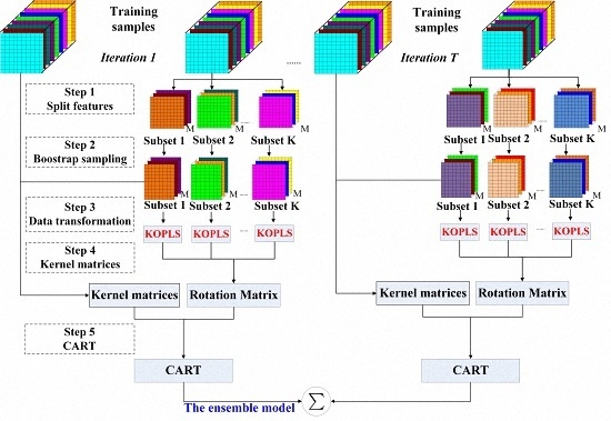
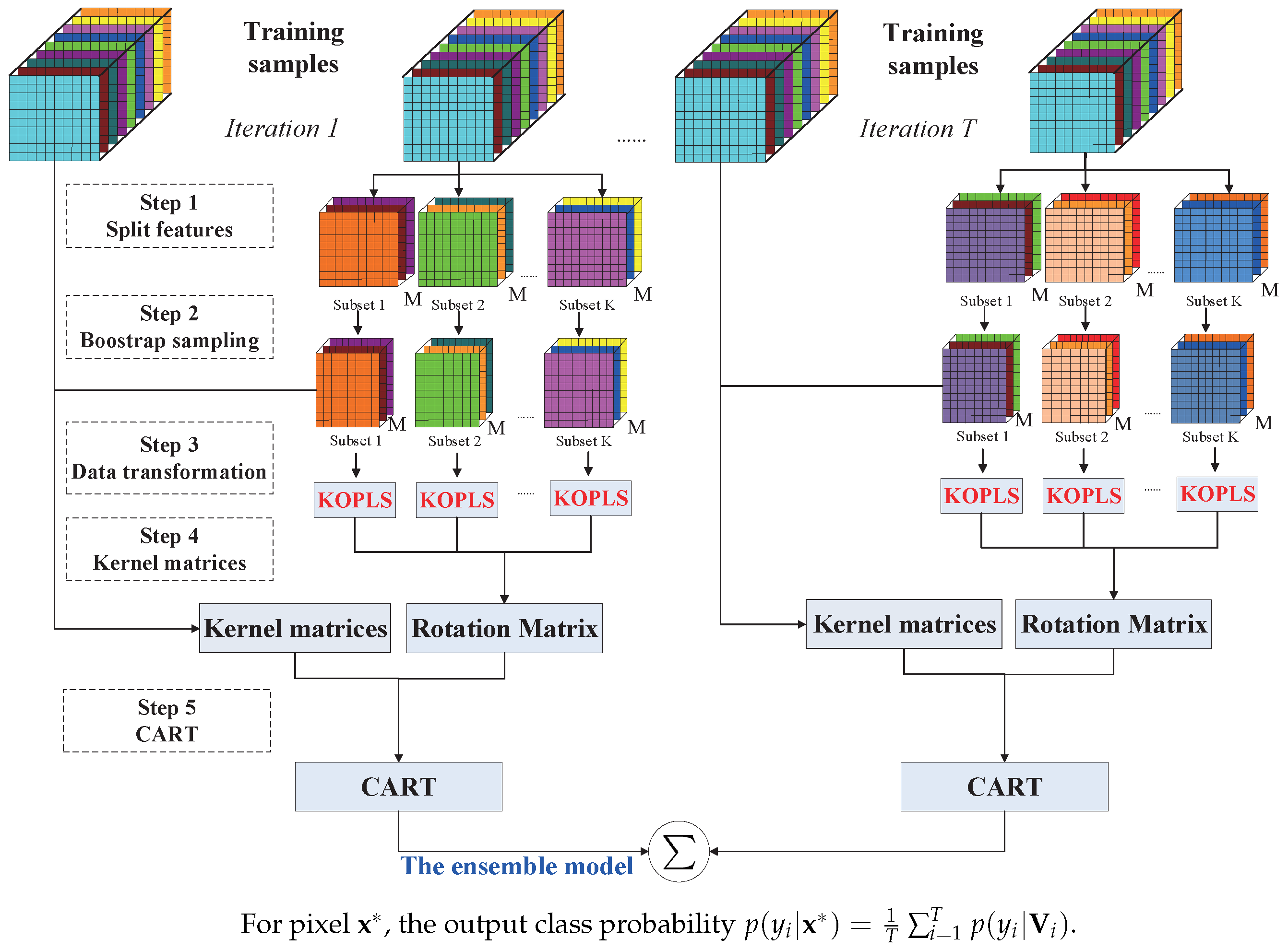
3.3. Rotation Forest with KOPLS

The success of MCSs (Multiple Classifier Systems) depend on not only the choice of base classifier, but also the diversity within the ensemble [12,44]. Aiming at improving both the diversity and classification accuracies of the DT classifiers within the ensemble, we propose a novel ensemble method, i.e., Rotation Forest with KOPLS (RoF-KOPLS), which aims at combining the advantages of KOPLS and RoF together. The proposed method can be summarized with the following steps (see Algorithm 2 and Figure 1). In the training phase, the feature space is randomly split into K disjoint subspace. For each subset, the initial training samples with 75% are drawn from the training data by using a bootstrap sampling method. KOPLS is applied to each subspace to get the coefficients R k . In the next step, the kernel matrices of X ^ i , j are calculated, and an individual classifier is trained on the extracted features F i n e w . In the prediction phase, the kernel matrices between X ^ i , j and a new sample x is generated firstly. Then, the new transformed dataset F i t e s t is classified by the ensemble, and the final result will be assigned to the corresponding class by the majority voting rule. We expect that RoF-KOPLS can improve the performance of RoF-OPLS by introducing further diversity by performing a kernel feature extraction within the ensemble. The base classifiers in RoF-KOPLS are expected to be more diverse compared to these in RoF-OPLS, thus yielding more powerful ensemble. Furthermore, depending on the types of kernel function, RoF-KOPLS can be more specific, i.e., RoF with linear kernel (RoF-KOPLS-Linear), RoF with polynomial kernel (RoF-KOPLS-Polynomial), and RoF with RBF kernel (RoF-KOPLS-RBF).
Algorithm 2 Rotation Forest with KOPLS
Training phase
Input: X , Y = x i , y i i = 1 l : training samples, T: number of classifiers, K: number of subsets, M: number of features in a subset, L: base classifier. The ensemble L = . F : Feature set
Output: The ensemble L
1:
for i = 1 : T do
2:
 randomly split the features F into K subsets F j i
3:
for j = 1 : K do
4:
  form the new training set X i , j with F j i
5:
  randomly select the 75% of the initial training samples to generate X ^ i , j
6:
  using KOPLS to transform X ^ i , j with the aim of getting the coefficients R i , j = α i , j 1 , , α i , j M
7:
  calculate the kernel matrices by X ^ i , j , Ktrain i , j = K ( X ^ i , j , X ^ i , j )
8:
end for
9:
 the features extracted will be given by: F i n e w = Ktrain i , 1 R i , 1 , , Ktrain i , K R i , K
10:
 train a DT classifier L i using F i n e w , Y
11:
 add the classifier to the current ensemble, L = L L i .
12:
end for
Prediction phase
Input: The ensemble L = L i i T . A new sample x . Rotation matrix: R .
Output: class label y
1:
for i = 1 : T do
2:
for j = 1 : K do
3:
  generate the kernel matrices between X ^ i , j and x , Ktest k = K ( X ^ i , j , x i , j )
4:
  generate the test features of x , F i t e s t = Ktest i , 1 R i , 1 , , Ktest i , k R i , K
5:
end for
6:
 run the classifier L i using F i t e s t as input
7:
end for
8:
calculate the confidence x for each class and assign the class label p ( y i | x ) = 1 T i = 1 T p ( y i | F i t e s t ) to the class with the largest confidence.

4. Experimental Results

Two popular hyperspectral airborne images were used for experiments. More detailed descriptions of the two data sets and the corresponding results are discussed in the next two subsections.
The following measures were used to evaluate the performances of different classification approaches:
  • Overall accuracy (OA) is the percentage of correctly classified pixels.
  • Average accuracy (AA) is the average of percentages of classified pixels for individual class.
  • Kappa coefficient (κ) is the percentage of agreement corrected by the level of agreement that would be expected by casually [23].
For the purpose of analysing the ensemble clearly, we adopted the following measures to estimate its performance.
  • Average of OA (AOA) is the average of OAs of individual classifiers within the ensemble.
  • Diversity in classifier ensemble. Diversity has been regarded as a very significant characteristic in classifier ensemble [45]. In this paper, coincident failure diversity (CFD) is used as the diversity measure [10]. The higher the value of CFD, the more diverse the ensemble.

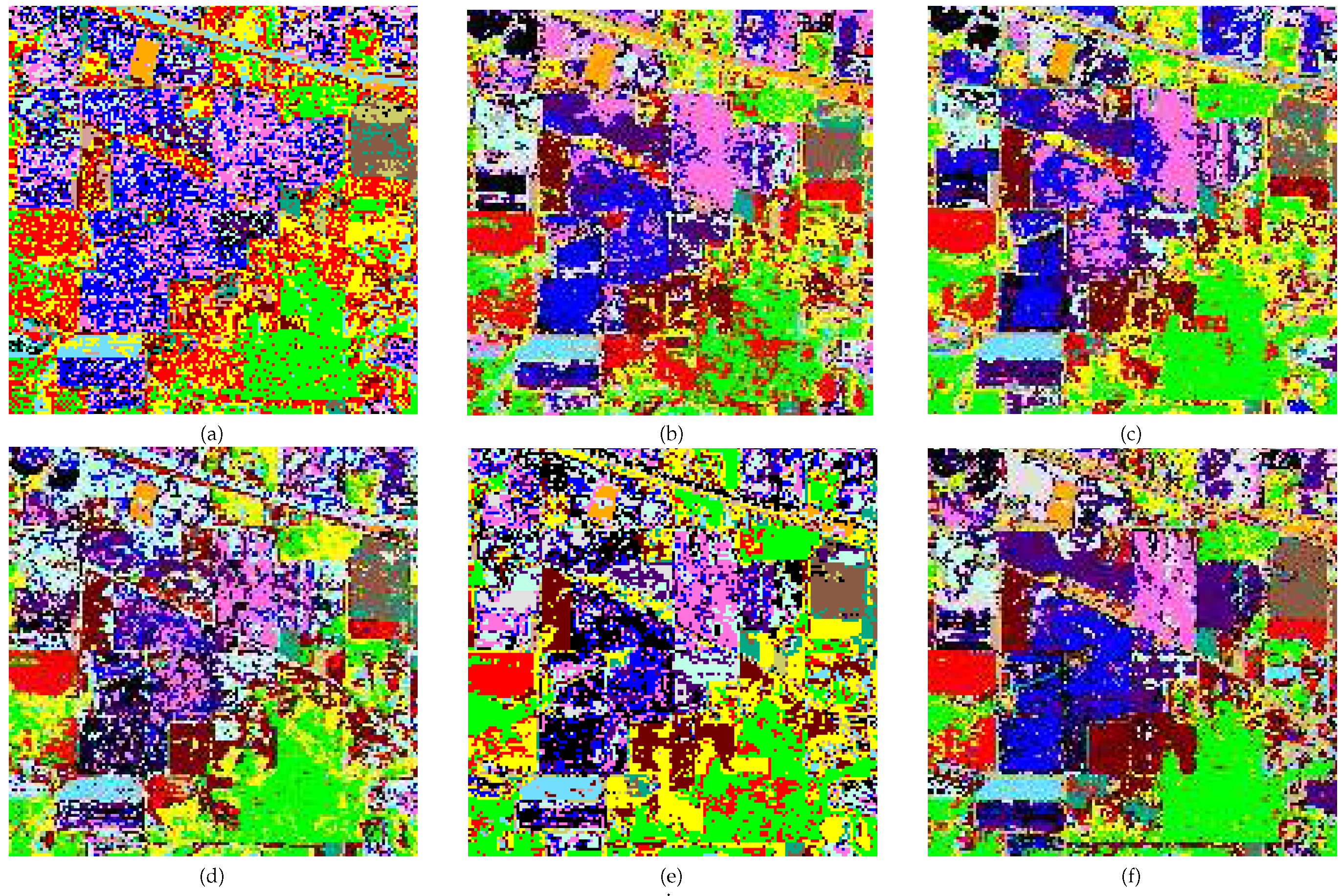
4.1. Results of the AVIRIS Indian Pines Image

The Indian Pines image was acquired by the Airborne Visible/Infrared Imaging Spectrometer (AVIRIS) sensors over the Indian Pines test site in Northwestern Indiana of an agricultural area. The image is 145 × 145 pixels, with a spatial resolution of 20 m per pixel. In order to evaluate the performance of our proposed methods, all full spectral bands, including 20 noisy and water absorption bands, was used for experiment. It is composed of 220 spectral channels in the wavelength ranging from 0.4 to 2.5 μm. Sixteen classes of interest are reported in Table 1. Figure 2 depicts the three-band false color composite image and the reference data of this image.
In order to evaluate the performance of the proposed classification techniques, some methods including support vector machine(SVMs), DT, RotBoost [46,47], DT with KOPLS (DT-KOPLS), and RoF-PCA were implemented for comparison. The reason why we select SVMs and DT in comparison to the proposed methods is that they are two of the leading classification techniques of hyperspectral data. As fa as SVM is concerned, the radial basis function kernel is choosen for classification, which include two parameters (i.e., penalty term C and the width of the exponential σ). Furthermore, in our experiments, fivefold cross-validation was used to select the best combination of parameters under the condition that C and σ were set to [ 2 4 , 2 12 ] and [ 2 10 , 2 5 ] , respectively. Furthermore, DT-KOPLS is the variant of DT. In terms of RoF-PCA, it is a ensemble method using independent DT built on a different set of extracted features. It is worth noting that the feature extraction for RoF-PCA is based on PCA. For DT-KOPLS, KOPLS is used for feature extraction prior to DT classifier. The range of extracted components is from 2 to 30. In this paper, three kernels, e.g., linear, RBF and polynomial, are used in KOPLS feature extraction prior to DT classifier. Only the best results are reported in this paper. The kernel width σ in RBF kernel was computed by the median of all pairwise distances between the samples [48], and c in polynomial kernel was set to 2. The reported results were achieved by averaging the results obtained from ten Monte Carlo runs. According to our previous studies [19,20], T is set to be 10 in the ensembles.
The number of features in a subset (M) is a crucial parameter for the Rotation Forest ensembles. In order to investigate the impact of M on the performance of different classification scheme, we randomly select a very limited training set, i.e., 10 samples per class. The evaluation of OA with the increase of M is depicted in Figure 3. It should be noted that, the value of M should be less than the number of classes for RoF-OPLS. For other methods, M ranges from 2 to 110. The results presented in Figure 3 obviously show that there is no consistent pattern of the relationship between M and OAs, which is in accordance with the conclusions obtained in our studies [20,49]. The OAs obtained by RoF-KOPLS-Linear and the RoF-KOPLS-Polynomial decrease as the increase of M. In particular, it is worth noting that the RoF-KOPLS-RBF can obtain the best OAs in all cases. Furthermore, RoF-KOPLS-RBF is insensitive to M in comparison with other classification methods when the value of M is greater the number of classes (i.e., 16). Another observation is that, the optimal values of M for different classification methods are various. For instance, RoF-KOPLS-RBF achieves the best classification result when M = 100. To ensure a fair comparison, the optimal values of M are independently selected for specific methods. Thus, the optimal values of M for RoF-OPLS, RoF-PCA, RoF-KOPLS-RBF, RoF-KOPLS-Linear, RoF-KOPLS-Polynomial were set to be 14, 100, 100, 4 and 4, respectively. Figure 4 plots the classification maps obtained by the individual and ensemble learning methods (only one Monte Carlo run).

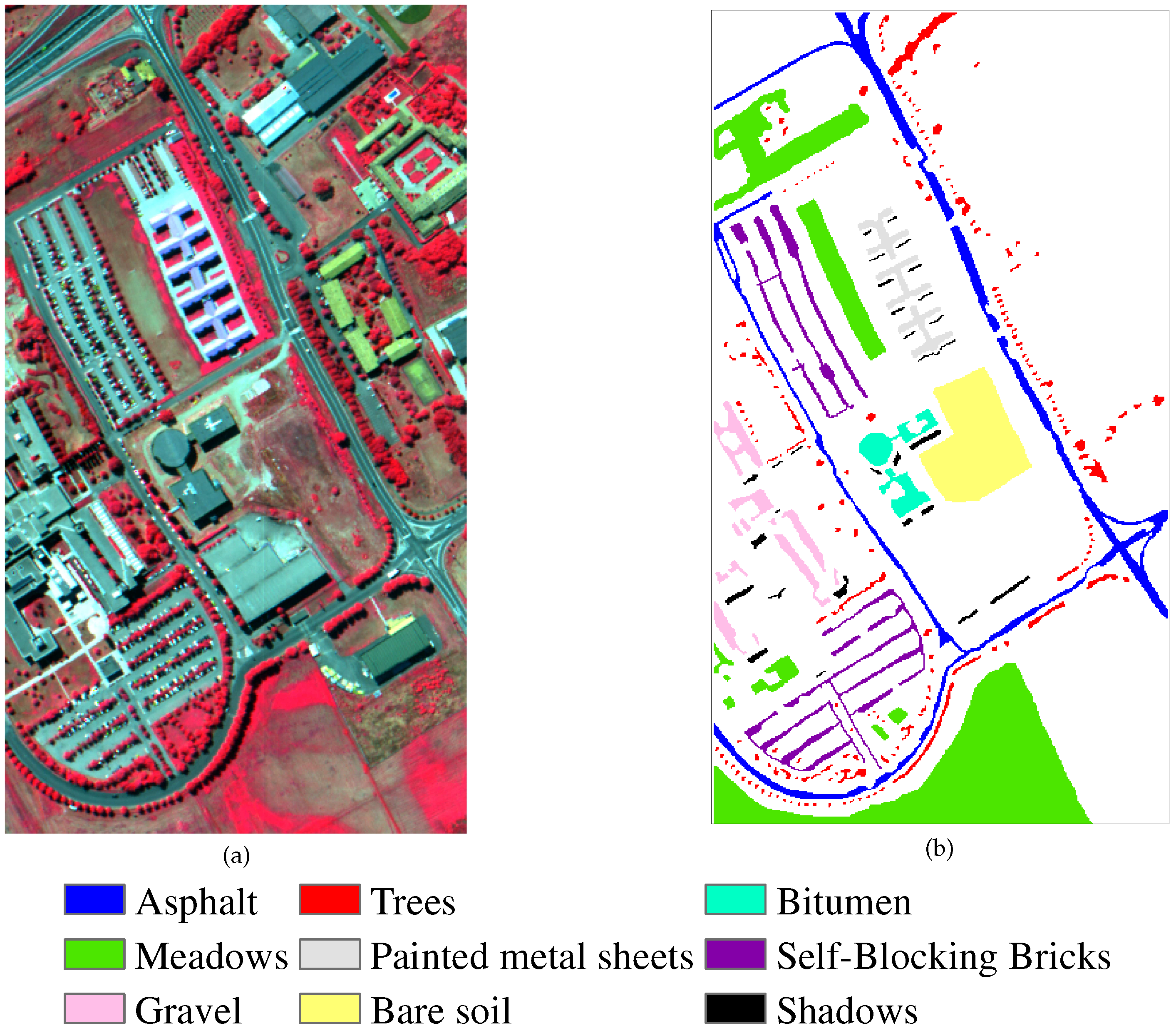
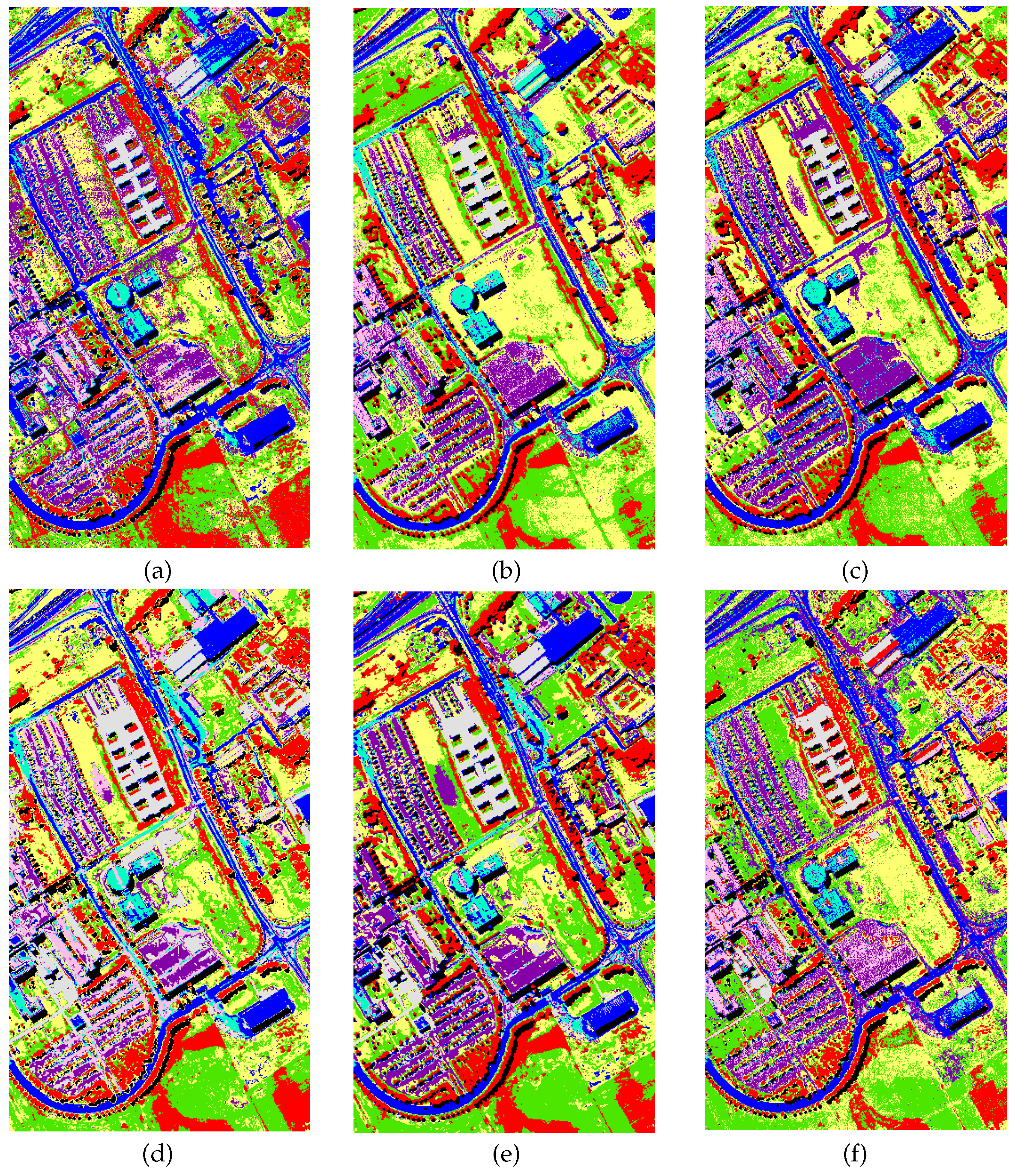
4.2. Results of the University of Pavia ROSIS Image
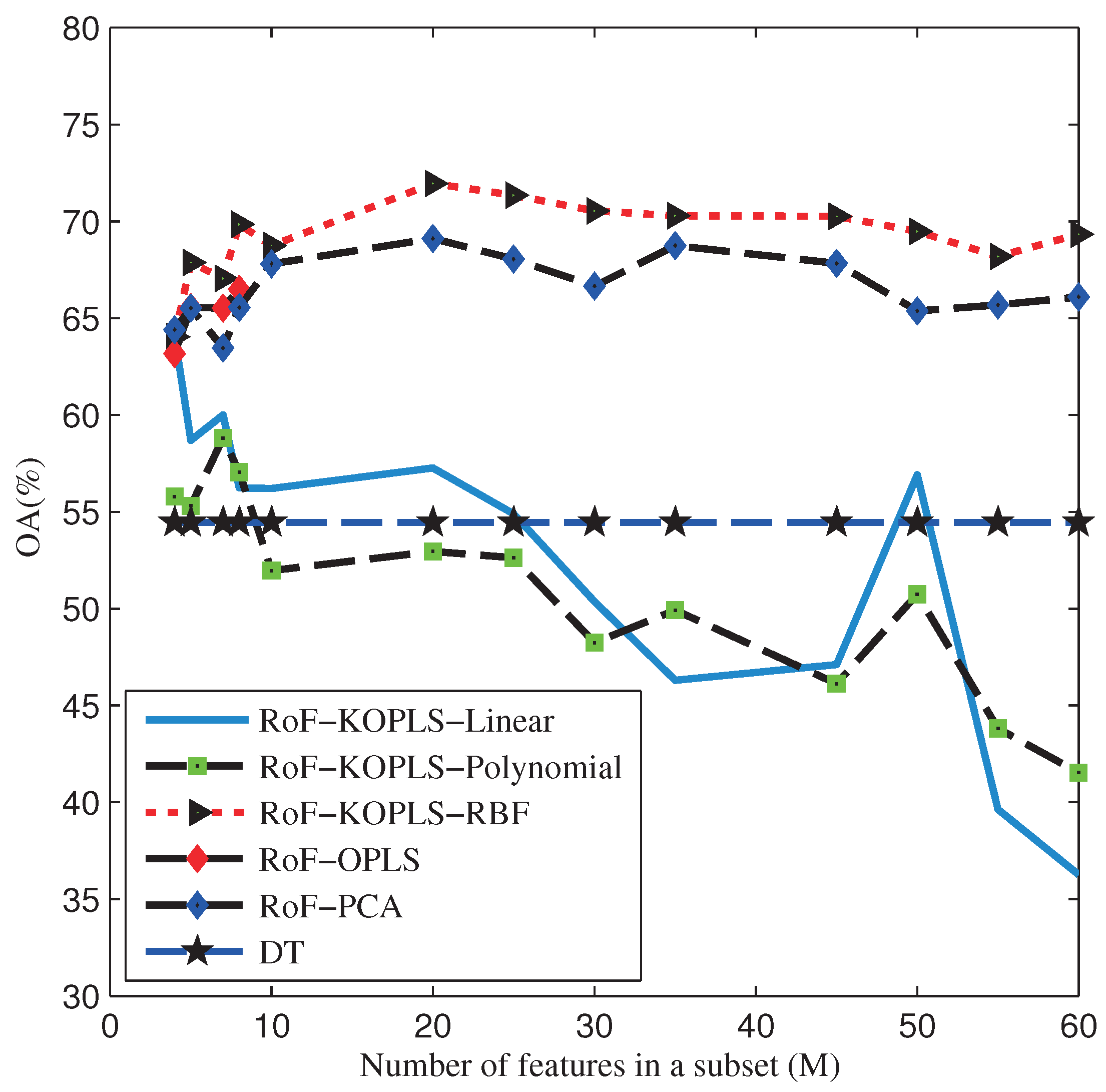
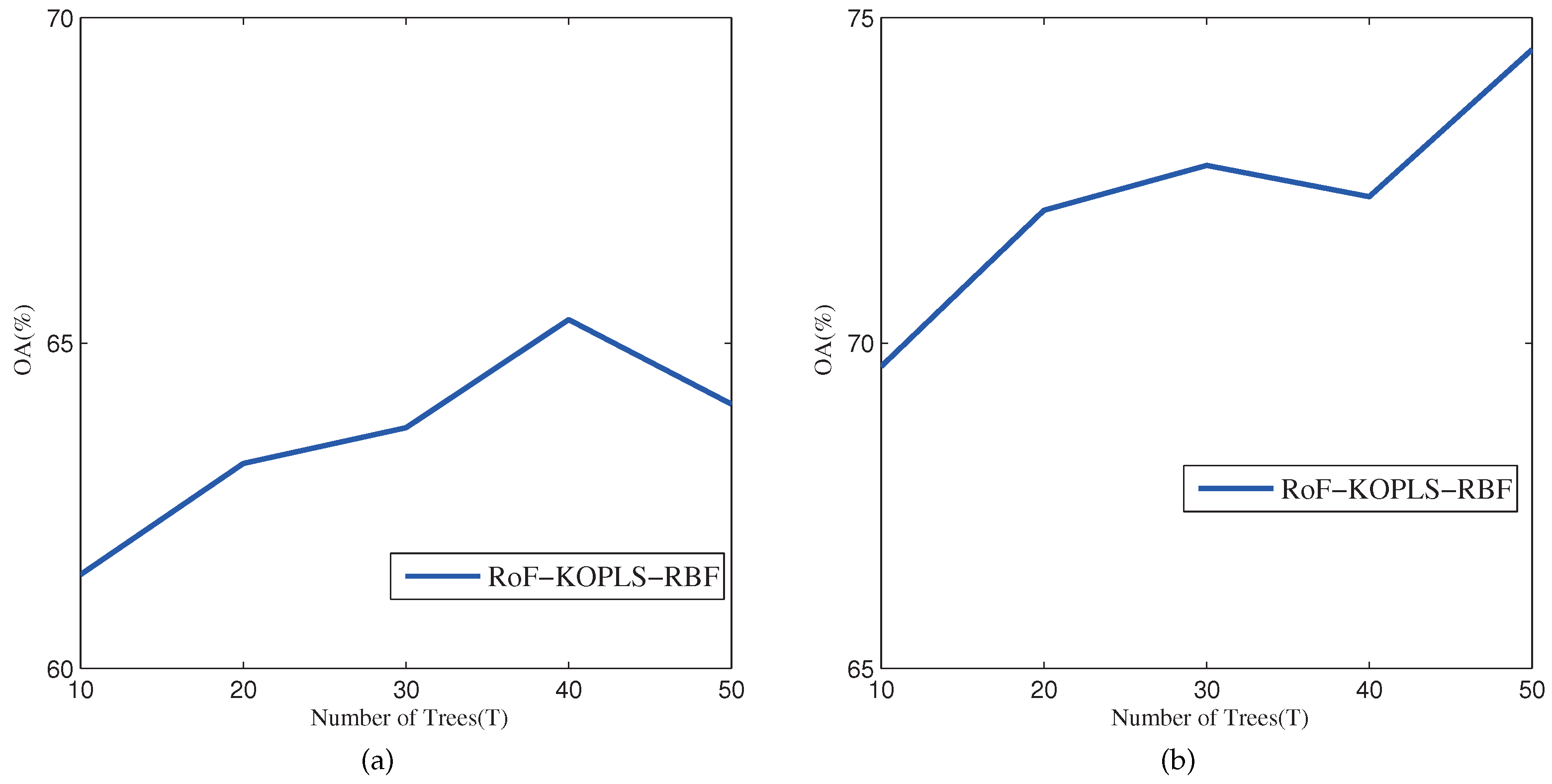
In the second study, the proposed scheme was tested on the ROSIS image, which is collected from an university area with a spatial resolution of 1.3 m and 103 bands. The original recorded image has a spatial dimension of 610 × 340 pixels, with 103 channels left for experiments by removing 12 noisy bands. Nine classes of interest are contained in the reference data with a total number of 42776 labeled samples. A false color composite image and the reference data are shown in Figure 5. For this experiment, we randomly select only 10 samples per class as training samples, which represents a very limited training set. In order to ensure a fair comparison, we conducted ten independent runs for each experiment in terms of training samples selection and classification.
In the first experiment, the impacts of M on the global accuracies obtained by all classification approaches were investigated. For the RoF-OPLS algorithm, the value of M should be less than the number of classes. Hence, the values of M were set to be 4, 5, 7 and 8. However, this limitation is not necessary for RoF-KOPLS and RoF-PCA methods. In order to clearly examine the effect of M on the OAs obtained by RoF-KOPLS and RoF-PCA methods, the value of M was set to the range from 4 to 60. Figure 6 shows the OAs obtained by different methods as a function of different values of M. Similar conclusion can be drawn with the former experiments. First, the performances of the RoF methods rely on the values of M. It should be noted that the RoF-KOPLS-RBF is insensitive to the value of M compared to other classification techniques when M is greater than 9 (i.e., the number of classes). Second, the impact of M on OA seems to be irregular. Third, the overall accuracies obtained by RoF-KOPLS-RBF are more accurate than those achieved by all other methods. Finally, the overall accuracies obtained by the RoF-KOPLS-Linear method and the RoF-KOPLS-Polynomial method exhibit larger variations as the increase of M. Nevertheless, the overall accuracies achieved by the presented RoF-KOPLS-RBF method tend to be stable with the increase of the value of M. In order to make fair comparisons, the value of M should be selected as the one achieving the best accuracy for each classification algorithm. In consequence, the values of RoF-OPLS, RoF-PCA, RoF-KOPLS-RBF, RoF-KOPLS-Linear, RoF-KOPLS-Polynomial were set to 8, 20, 20, 4 and 7, respectively. Figure 7 depicts the classification maps obtained by all the considered methods.

5. Discussion

5.1. Discussion on the AVIRIS Indian Pines Image

The overall and class-specific accuracies of different classification algorithms are presented in Table 1. The results reveal that the classifier ensembles can yield more accurate accuracies compared to single classifiers. It is apparent that the proposed RoF-KOPLS-RBF method provides good results roughly equivalent to the recently proposed method, Rotboost, which is followed by RoF-PCA and RoF-OPLS. Furthermore, it should be noted that the proposed RoF-KOPLS-RBF method can achieve considerable increases in most class-specific accuracies, which significantly outperforms others. The McNemar’s test revealed that the difference between RoF-KOPLS-RBF and RoF-OPLS are statistically significant (|z| > 1.96) [50]. The kernel-based method improves the accuracies by 8.06% in OA and 6.16% in AA. Furthermore, as we can see from the Figure 4, the Rotation Forest ensembles can improve the classification accuracies and produce more smooth classification maps. These results validate the good performance of the proposed RoF-KOPLS-RBF by combining KOPLS and RoF.
The number of classifiers (T) and training samples are the key parameters for the proposed method. In order to investigate the influence of T on the classification accuracies, we have performed the classification results when the number of feature in a subset M is set to 100. As we can see from the Figure 8a, the classification accuracies are improved with the increase of T.
Table 2 presents classification accuracies obtained by individual classifier using different numbers of training samples. As reported in the table, the proposed RoF-KOPLS-RBF, RoF-KOPLS-Linear, RoF-KOPLS-Polynomial, and RoF-OPLS methods are superior to DT and DT-KOPLS. RoF-KOPLS-RBF, RoF-OPLS, and RoF-PCA achieve better classification accuracies when compared to SVM. It can be found that the proposed RoF-KOPLS-RBF method gains the best classification results under most of training scenarios as compared to other classification techniques. As we can see from the Table 2, when we compare the proposed method with the recently new classification method RotBoost, our proposed method is equivalent or superior to the RotBoost approach. Therefore, it can be concluded that RoF-KOPLS-RBF works more efficiently with relatively low number of labeled training samples.
Table 3 provides the OAs, AOAs, and diversities obtained by different RoF ensembles using 10 samples for each class. The accuracy of individual classifier and diversity are two important properties for a classifier ensemble as higher values of AOA and diversity always give rise to better performance. The results in this table show that the proposed RoF-KOPLS-RBF method acquires the highest AOA and diversity, leading to the best classification accuracies. Furthermore, it is worth noting that the effect of kernel functions on the classification accuracies are significant. RoF-KOPLS-RBF method obtains better classification results in comparison to RoF-KOPLS-Linear and RoF-KOPLS-Polynomial methods. This can be attributed to RoF-KOPLS-RBF’s higher values of AOA and diversity.

5.2. Discussion on the University of Pavia ROSIS Image

The classification accuracies of all the classification techniques are summarized in Table 4. From this table, the best OA, kappa coefficient, and class-specific accuracies for most classes are achieved by the presented RoF-KOPLS-RBF method, which is followed by the RotBoost, RoF-PCA and RoF-OPLS approach. In this case, the OA of the RoF-OPLS approach is improved by 5.46% compared to the RoF-KOPLS-RBF. According to the results of McNemar’s test, the RoF-KOPLS-RBF classification map is significantly more accurate compared to those achieved by other methods except the RotBoost approach with a confident level of 5%. We can conclude that the proposed RoF-KOPLS-RBF method inherits the good merits of KOPLS and RoF, thus leading to improved classification result.
As like in the first experiment, the impacts of T and training samples on the classification results have also been explored. When investigating the influence of T on the classification accuracies, the number of feature in a subset M is set to 20 achieving the best accuracy for the proposed method. Figure 8b shows the OA (%) using different number of T. With the increase of T, the classification results are significantly improved. Table 5 gives the OAs and AAs (in parentheses) obtained by different classification approaches when using different number of training samples. As expected, the classification accuracies obtained by all methods becomes higher with the increase of the training set size. Analogous to the first experiment, the proposed RoF-KOPLS-RBF method demonstrates relatively higher performance with a very limited number of training samples in terms of OAs and AAs, as compared to the other classification approaches. Moreover, from Figure 7, we can draw that the Rotation Forest ensembles generate more accurate classification maps with reduced data noise in comparison with the individual classifiers.
The OAs, AOAs, and diversities obtained by Rotation Forest ensembles are reported in Table 6 to evaluate the ensemble clearly. It can be noted that the proposed RoF-KOPLS-RBF approach gives the highest AOA and diversity, when compared to other classification approaches. RoF-KOPLS-RBF gains the best overall accuracy due to the fact that higher AOA and diversity lead to better ensemble performance, which confirms the validity of combining the merits of KOPLS and Rotation Forest. As can be seen from the table, we can conclude that the kernel function can give rise to significant impact on the classification accuracies, which is similar to the first experiment. RoF-KOPLS-RBF achieves the higher values of AOA and diversity when compared to RoF-KOPLS-Linear and RoF-KOPLS-Polynomial, leading to better classification results.
In addition, it should be noted that although the proposed method has shown good performance in the classification of hyperspectral data, it is confronted with some common cons for Rotation Forest, e.g., the relative low computational efficiency and sensitivity to the number of features in a subset [21]. Moreover, the proposed method only consider the spectral information so that it obtains suboptimal classification results when compared to the method taking advantage of the spatial and spectral information simultaneously [20].

6. Conclusions

In this paper, a new classification approach is presented by combining the advantages of kernel-based feature extraction, i.e., KOPLS, and ensemble method, i.e., Rotation Forest. The performance of the proposed methods was evaluated by several experiments based on two popular hyperspectral images. Experimental results demonstrated that the proposed RoF-KOPLS methodology can inherit the merits of RoF and KOPLS to achieve more accurate classification results.
The following conclusions can be drawn according to the experimental results:
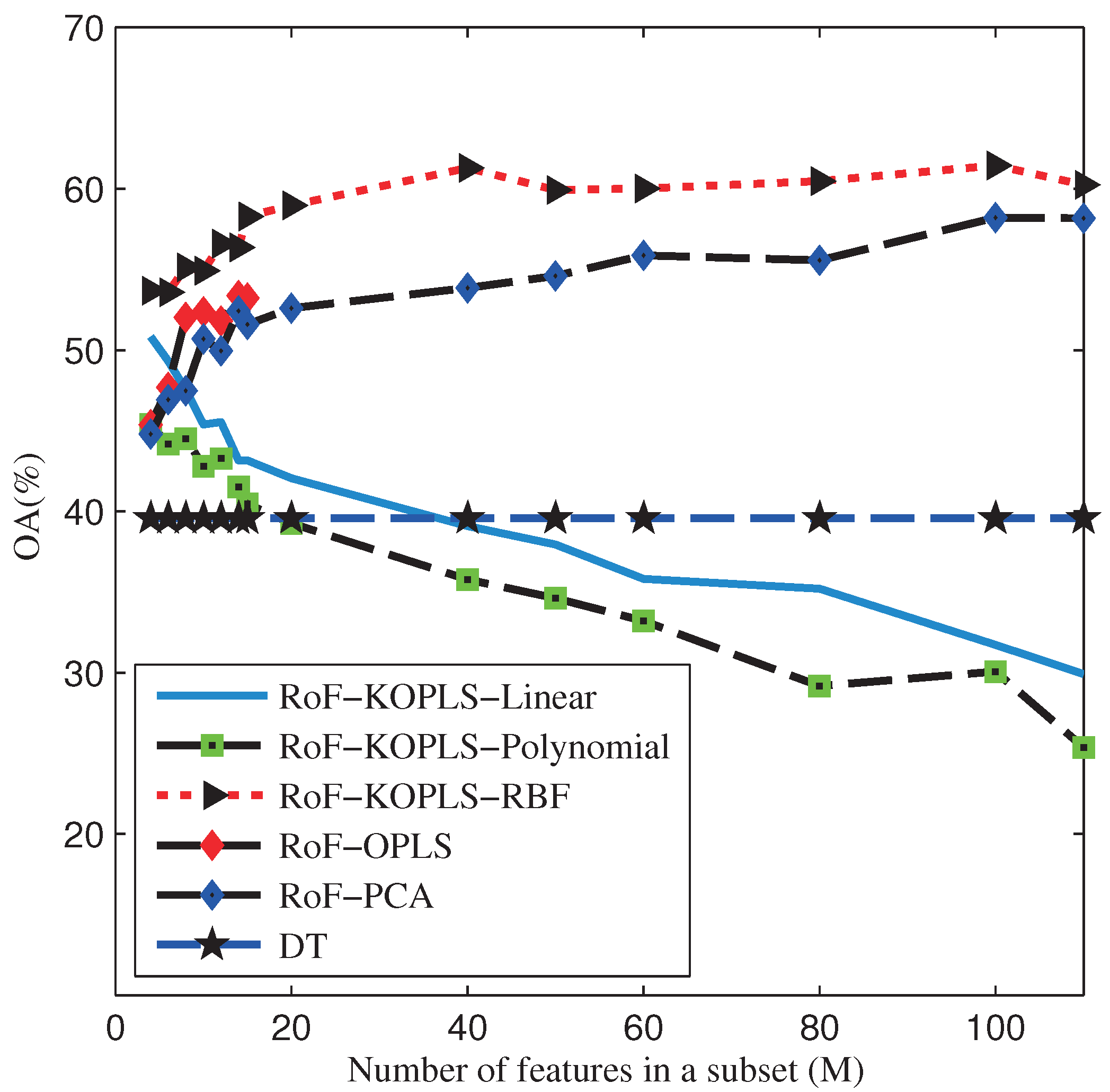
  • RoF-KOPLS with RBF kernel yields the best accuracies against the comparative methods above-mentioned due to the ability of improving the accuracy of base classifiers and the diversity within the ensemble, especially for the very limited training set.
  • In RoF-KOPLS, the kernel functions can give rise to significant influences on the classification results. Experimental results have shown that RoF-KOPLS with RBF kernel obtained the best performances.
  • RoF-KOPLS with RBF kernel is insensitive to the number of features in a subset when compared to other methods.
In the future, we will further explore the integration of Rotation Forest and kernel methods in classifier ensemble for real application of the hyperspectral images. On the one hand, we will attempt to combine the proposed method with Adaboost or Bagging [51]. On the other hand, given the important role of spatial features in the classification of hyperspectral image [52], spatial information will be incorporated to improve the performances of the proposed classification scheme in the following work.

Acknowledgments

This work is partially supported by the Natural Science Foundation of China (No. 41171323), Jiangsu Provincial Natural Science Foundation (No. BK2012018) and National Key Scientific Instrument and Equipment Development Program (No. 012YQ050250). The authors would like to thank D. Landgrebe from Purdue University for providing the AVIRIS hyperspectral data and P. Gamba for providing the University of Pavia ROSIS Image, along with the training and test data sets.

Author Contributions

Jike Chen and Junshi Xia conceived and designed the experiments; Jike Chen performed the experiments, analyzed the data and wrote the paper. Peijun Du, Jocelyn Chanussot, Zhaohui Xue and Xiangjian Xie gave comments, suggestions to the manuscript and checked the writing.

Conflicts of Interest

The authors declare no conflict of interest.

Abbreviations

The following abbreviations are used in this manuscript:
PCAPrinciple Component Analysis
RBFRadial Basis Function
FLDAFisher’s Linear Discriminant Analysis
PLSPartial Least Square Regression
OPLSOrthonormalized Partial Least Square Regression
KOPLSKernel Orthonormalized Partial Least Square Regression
RFRandom Forest
SVMsSupport Vector Machines
RoFRotation Forest
DTDecision Trees
CARTClassification and Regression Tree
RoF-OPLSRotation Forest with OPLS
RoF-KOPLSRotation Forest with KOPLS
OAOverall Accuracy
AAAverage Accuracy
AOAAverage of OA
κKappa coefficient
CFDCoincident Failure Diversity
RotBoostRotation Forest with Adaboost
DT-KOPLSDT with KOPLS

References

  1. Plaza, A.; Benediktsson, J.A.; Boardman, J.W.; Brazile, J.; Bruzzone, L.; Camps-Valls, G.; Chanussot, J.; Fauvel, M.; Gamba, P.; Gualtieri, A.; et al. Recent advances in techniques for hyperspectral image processing. Remote Sens. Environ. 2009, 113, S110–S122. [Google Scholar] [CrossRef]
  2. Shang, X.; Chisholm, L.A. Classification of Australian native forest species using hyperspectral remote sensing and machine-learning classification algorithms. IEEE J. Sel. Top. Appl. Earth Obs. Remote Sens. 2014, 7, 2481–2489. [Google Scholar] [CrossRef]
  3. Bioucas-Dias, J.M.; Plaza, A.; Camps-Valls, G.; Scheunders, P.; Nasrabadi, N.M.; Chanussot, J. Hyperspectral remote sensing data analysis and future challenges. IEEE Geosci. Remote Sens. Mag. 2013, 1, 6–36. [Google Scholar] [CrossRef]
  4. Manolakis, D.; Marden, D.; Shaw, G.A. Hyperspectral image processing for automatic target detection applications. Lincoln Lab. J. 2003, 14, 79–116. [Google Scholar]
  5. Dong, Y.; Zhang, L.; Zhang, L.; Du, B. Maximum margin metric learning based target detection for hyperspectral images. ISPRS J. Photogramm. Remote Sens. 2015, 108, 138–150. [Google Scholar] [CrossRef]
  6. Hughes, G. On the mean accuracy of statistical pattern recognizers. IEEE Trans. Inf. Theory 1968, 14, 55–63. [Google Scholar] [CrossRef]
  7. Oza, N.C.; Tumer, K. Classifier ensembles: Select real-world applications. Inf. Fusion 2008, 9, 4–20. [Google Scholar] [CrossRef]
  8. Benediktsson, J.A.; Chanussot, J.; Fauvel, M. Multiple classifier systems in remote sensing: From basics to recent developments. In Multiple Classifier Systems; Springer: Berlin, Germany, 2007; pp. 501–512. [Google Scholar]
  9. Du, P.; Xia, J.; Zhang, W.; Tan, K.; Liu, Y.; Liu, S. Multiple classifier system for remote sensing image classification: A review. Sensors 2012, 12, 4764–4792. [Google Scholar] [CrossRef] [PubMed]
  10. Kuncheva, L.I.; Whitaker, C.J. Measures of diversity in classifier ensembles and their relationship with the ensemble accuracy. Mach. Learn. 2003, 51, 181–207. [Google Scholar] [CrossRef]
  11. Shipp, C.A.; Kuncheva, L.I. Relationships between combination methods and measures of diversity in combining classifiers. Inf. Fusion 2002, 3, 135–148. [Google Scholar] [CrossRef]
  12. Kuncheva, L.I. Combining Pattern Classifiers: Methods and Algorithms; John Wiley & Sons: Hoboken, NJ, USA, 2004. [Google Scholar]
  13. Rokach, L. Pattern Classification Using Ensemble Methods; World Scientific: Singapore, Singapore, 2009; Volume 75. [Google Scholar]
  14. Waske, B.; Braun, M. Classifier ensembles for land cover mapping using multitemporal SAR imagery. ISPRS J. Photogramm. Remote Sens. 2009, 64, 450–457. [Google Scholar] [CrossRef]
  15. Briem, G.J.; Benediktsson, J.A.; Sveinsson, J.R. Multiple classifiers applied to multisource remote sensing data. IEEE Trans. Geosci. Remote Sens. 2002, 40, 2291–2299. [Google Scholar] [CrossRef]
  16. Pal, M. Random forest classifier for remote sensing classification. Int. J. Remote Sens. 2005, 26, 217–222. [Google Scholar] [CrossRef]
  17. Rodriguez, J.J.; Kuncheva, L.I.; Alonso, C.J. Rotation forest: A new classifier ensemble method. IEEE Trans. Pattern Anal. Mach. Intell. 2006, 28, 1619–1630. [Google Scholar] [CrossRef] [PubMed]
  18. Xia, J.; Chanussot, J.; Du, P.; He, X. Rotation-Based Ensemble Classifiers for High-Dimensional Data. In Fusion in Computer Vision; Springer: Berlin, Germany, 2014; pp. 135–160. [Google Scholar]
  19. Xia, J.; Du, P.; He, X.; Chanussot, J. Hyperspectral remote sensing image classification based on rotation forest. IEEE Geosci. Remote Sens. Lett. 2014, 11, 239–243. [Google Scholar] [CrossRef]
  20. Xia, J.; Chanussot, J.; Du, P.; He, X. Spectral–Spatial Classification for Hyperspectral Data Using Rotation Forests with Local Feature Extraction and Markov Random Fields. IEEE Trans. Geosci. Remote Sens. 2015, 53, 2532–2546. [Google Scholar] [CrossRef]
  21. Du, P.; Samat, A.; Waske, B.; Liu, S.; Li, Z. Random Forest and Rotation Forest for fully polarized SAR image classification using polarimetric and spatial features. J. Photogramm. Remote Sens. 2015, 105, 38–53. [Google Scholar] [CrossRef]
  22. Hsu, P.H. Feature extraction of hyperspectral images using wavelet and matching pursuit. ISPRS J. Photogramm. Remote Sens. 2007, 62, 78–92. [Google Scholar] [CrossRef]
  23. Richards, J.A. Remote Sensing Digital Image Analysis; Springer: Berlin, Germany, 1999; Volume 3. [Google Scholar]
  24. Hotelling, H. Analysis of a complex of statistical variables into principal components. J. Educ. Psychol. 1933, 24, 417. [Google Scholar] [CrossRef]
  25. Plaza, A.; Martinez, P.; Plaza, J.; Perez, R. Dimensionality reduction and classification of hyperspectral image data using sequences of extended morphological transformations. IEEE Trans. Geosci. Remote Sens. 2005, 43, 466–479. [Google Scholar] [CrossRef]
  26. Fukunaga, K. Introduction to Statistical Pattern Recognition; Academic Press: New York, NY, USA, 2013. [Google Scholar]
  27. Wold, S.; Albano, C.; Dunn, W.J., III; Edlund, U.; Esbensen, K.; Geladi, P.; Hellberg, S.; Johansson, E.; Lindberg, W.; Sjöström, M. Multivariate data analysis in chemistry. In Chemometrics; Springer: Berlin, Germany, 1984; pp. 17–95. [Google Scholar]
  28. Worsley, K.J.; Poline, J.B.; Friston, K.J.; Evans, A. Characterizing the response of PET and fMRI data using multivariate linear models. NeuroImage 1997, 6, 305–319. [Google Scholar] [CrossRef] [PubMed]
  29. Du, Q. Modified Fisher’s linear discriminant analysis for hyperspectral imagery. IEEE Geosci. Remote Sens. Lett. 2007, 4, 503–507. [Google Scholar] [CrossRef]
  30. Barker, M.; Rayens, W. Partial least squares for discrimination. J. Chemom. 2003, 17, 166–173. [Google Scholar] [CrossRef]
  31. Arenas-García, J.; Camps-Valls, G. Efficient kernel orthonormalized PLS for remote sensing applications. IEEE Trans. Geosci. Remote Sens. 2008, 46, 2872–2881. [Google Scholar] [CrossRef]
  32. Arenas-García, J.; Petersen, K.; Camps-Valls, G.; Hansen, L.K. Kernel multivariate analysis framework for supervised subspace learning: A tutorial on linear and kernel multivariate methods. J. Educ. Psychol. 2013, 30, 16–29. [Google Scholar] [CrossRef]
  33. Leiva-Murillo, J.M.; Artés-Rodríguez, A. Maximization of mutual information for supervised linear feature extraction. IEEE Trans. Neural Netw. 2007, 18, 1433–1441. [Google Scholar] [CrossRef] [PubMed]
  34. Arenas-García, J.; Camps-Valls, G. Feature extraction from remote sensing data using Kernel Orthonormalized PLS. In Proceedings of the IEEE International Geoscience and Remote Sensing Symposium (IGARSS 2007), Barcelona, Spain, 23–28 July 2007; pp. 258–261.
  35. Persello, C.; Bruzzone, L. Kernel-Based Domain-Invariant Feature Selection in Hyperspectral Images for Transfer Learning. IEEE Trans. Geosci. Remote Sens. 2016, 54, 2615–2626. [Google Scholar] [CrossRef]
  36. Camps-Valls, G.; Mooij, J.; Schölkopf, B. Remote sensing feature selection by kernel dependence measures. IEEE Geosci. Remote Sens. Lett. 2010, 7, 587–591. [Google Scholar] [CrossRef]
  37. Jiménez-Rodríguez, L.O.; Arzuaga-Cruz, E.; Vélez-Reyes, M. Unsupervised linear feature-extraction methods and their effects in the classification of high-dimensional data. IEEE Trans. Geosci. Remote Sens. 2007, 45, 469–483. [Google Scholar] [CrossRef]
  38. Arenas-Garcıa, J.; Petersen, K.B.; Hansen, L.K. Sparse kernel orthonormalized PLS for feature extraction in large data sets. Adv. Neural Inf. Process. Syst. 2007, 19, 33–40. [Google Scholar]
  39. Breiman, L.; Friedman, J.; Stone, C.J.; Olshen, R.A. Classification and Regression Trees; CRC Press: Boca Raton, FL, USA, 1984. [Google Scholar]
  40. Roweis, S.; Brody, C. Linear Heteroencoders; Gatsby Computational Neuroscience Unit, Alexandra House: London, UK, 1999. [Google Scholar]
  41. Shawe-Taylor, J.; Cristianini, N. Kernel Methods for Pattern Analysis; Cambridge University Press: Cambridge, UK, 2004. [Google Scholar]
  42. Camps-Valls, G. Kernel Methods in Bioengineering, Signal and Image Processing; Igi Global: Hershey, PA, USA, 2006. [Google Scholar]
  43. Rosipal, R.; Trejo, L.J. Kernel partial least squares regression in reproducing kernel hilbert space. J. Mach. Learn. Res. 2002, 2, 97–123. [Google Scholar]
  44. Ranawana, R.; Palade, V. Multi-Classifier Systems: Review and a roadmap for developers. Inf. Fusion 2006, 3, 1–41. [Google Scholar] [CrossRef]
  45. Cunningham, P.; Carney, J. Diversity versus quality in classification ensembles based on feature selection. In Machine Learning: ECML 2000; Springer: Berlin, Germany, 2000; pp. 109–116. [Google Scholar]
  46. Zhang, C.X.; Zhang, J.S. RotBoost: A technique for combining Rotation Forest and AdaBoost. Pattern Recog. Lett. 2008, 29, 1524–1536. [Google Scholar] [CrossRef]
  47. Li, F.; Xu, L.; Siva, P.; Wong, A.; Clausi, D.A. Hyperspectral Image Classification With Limited Labeled Training Samples Using Enhanced Ensemble Learning and Conditional Random Fields. IEEE J. Sel. Top. Appl. Earth Obs. Remote Sens. 2015, 8, 2427–2438. [Google Scholar] [CrossRef]
  48. Blaschko, M.B.; Shelton, J.A.; Bartels, A.; Lampert, C.H.; Gretton, A. Semi-supervised kernel canonical correlation analysis with application to human fMRI. Inf. Fusion 2011, 32, 1572–1583. [Google Scholar] [CrossRef]
  49. Xia, J.; Mura, M.D.; Chanussot, J.; Du, P.; He, X. Random Subspace Ensembles for Hyperspectral Image Classification with Extended Morphological Attribute Profiles. IEEE Trans. Geosci. Remote Sens. 2015, 53, 4768–4786. [Google Scholar] [CrossRef]
  50. Foody, G.M. Thematic map comparison. Photogramm. Eng. Remote Sens. 2004, 70, 627–633. [Google Scholar] [CrossRef]
  51. Li, F.; Wong, A.; Clausi, D.A. Combining rotation forests and adaboost for hyperspectral imagery classification using few labeled samples. In Proceedings of the 2014 IEEE International Geoscience and Remote Sensing Symposium (IGARSS), Quebec City, QC, Canada, 13–18 July 2014; pp. 4660–4663.
  52. Fauvel, M.; Tarabalka, Y.; Benediktsson, J.A.; Chanussot, J.; Tilton, J.C. Advances in spectral-spatial classification of hyperspectral images. Proc. IEEE 2013, 101, 652–675. [Google Scholar] [CrossRef]
Figure 1. Illustration of the RoF-KOPLS.
Remotesensing 08 00601 g001
Figure 2. AVIRIS Indian Pines data set. (a) Three-band color composite (bands 57, 27, 17); (b) Ground-truth map containing 16 mutually exclusive land-cover classes. The legend of this scene is shown at the bottom.
Remotesensing 08 00601 g002
Figure 3. Indian Pines AVIRIS Image. OAs obtained by DT, RoF-PCA, RoF-OPLS, RoF-KOPLS-Linear, RoF-KOPLS-Polynomial, RoF-KOPLS-RBF with different number of M.
Remotesensing 08 00601 g003
Figure 4. Classification maps of the Indian Pines AVIRIS image (only one Monte Carlo run). OAs of the classifiers are presented as follows: (a) DT (40.20%); (b) RoF-PCA (57.39%); (c) RoF-OPLS (54.97%); (d) RoF-KOPLS-Linear (45.39%); (e) RoF-KOPLS-Polynomial (42.80%); (f) RoF-KOPLS-RBF (64.25%)
Remotesensing 08 00601 g004
Figure 5. ROSIS University of Pavia data set. (a) Three-band color composite (bands 102, 56, 31); (b) Reference map containing 9 mutually exclusive land-cover classes. The legend of this scene is shown at the bottom.
Remotesensing 08 00601 g005
Figure 6. OAs obtained by DT, RoF-PCA, RoF-OPLS, RoF-KOPLS-Linear, RoF-KOPLS-Polynomial, RoF-KOPLS-RBF with different number of M from the University of Pavia ROSIS Image.
Remotesensing 08 00601 g006
Figure 7. Classification maps of the University of Pavia ROSIS image (only one Monte Carlo run). OAs of the classifiers are presented as follows: (a) DT (54.06%); (b) RoF-PCA (66.0%); (c) RoF-OPLS (65.24%); (d) RoF-KOPLS-Linear (57.26%); (e) RoF-KOPLS-Polynomial (60.57%); (f) RoF-KOPLS-RBF (70.65%).
Remotesensing 08 00601 g007
Figure 8. Sensitivity to the change of the number of trees. (a) Indian Pines AVIRIS image; (b) University of Pavia ROSIS image.
Remotesensing 08 00601 g008
Table 1. Overall, Average and Class-specific Accuracies for the Indian Pines AVIRIS image.
ClassTrainTestSVMDTRotBoostDT-KOPLSRoF-PCARoF-OPLSRoF-KOPLS
RBFLinearPolynomial
Alfalfa105476.3074.8182.5042.4185.9186.1189.8181.8573.52
Corn-no till10143427.3329.8756.6411.0552.0146.6953.1839.5232.36
Corn-min till1083433.3926.6250.8516.9450.6945.3047.2844.4436.02
Bldg-Grass-Tree-Drives1023456.3726.7975.008.55066.1673.5567.3149.1545.68
Grass/pasture1049753.7657.2476.1834.3571.1772.7278.1769.7269.72
Grass/trees1074760.8340.1383.8826.0581.3874.6688.5969.6564.79
Grass/pasture-mowed102690.7782.6990.6368.0891.8792.3195.0091.5487.31
Corn1048951.7649.2882.1525.0178.0464.3487.8367.7162.35
Oats102094.0083.5096.0050.5095.0095.00100.089.5087.50
Soybeans-no till1096845.6131.2467.1217.0762.2154.3255.5152.3640.19
Soybeans-min till10246834.8930.0643.0017.3241.1729.1141.1734.8531.67
Soybeans-clean till1061432.9824.9248.6614.6645.1540.5456.8131.8923.21
Wheat1021293.5484.9596.6350.0994.7095.6198.4989.2587.36
Woods10129467.6768.6380.0237.3373.7580.0283.7973.2270.83
Hay-windrowed1038029.7635.0338.0811.3443.3845.1852.5038.5330.82
Stone-steel towers109588.0089.6897.4164.4295.2992.2190.8491.5892.63
OA44.7339.5661.5021.5558.2953.3861.4450.8345.40
AA58.5652.2272.8030.9570.4967.9874.1463.4258.50
κ38.6533.1757.0314.6253.5248.2156.9845.3839.53
Table 2. OAs and AAs (in Parentheses) Obtained for Different Classification Methods When Applied to the Indian Pines AVIRIS image.
Samples Per ClassSVMDTRotBoostDT-KOPLSRoF-PCARoF-OPLSRoF-KOPLS
RBFLinearPolynomial
1044.73 (58.56)39.56 (52.22)61.50 (72.80)21.55 (30.95)58.29 (70.49)53.38 (67.98)61.44 (74.14)50.83 (63.42)45.40 (58.50)
2055.45 (68.76)44.48 (58.01)68.34 (77.97)22.74 (32.89)65.32 (77.01)61.28 (74.67)67.40 (79.38)59.44 (71.25)53.31 (66.80)
3060.81 (73.23)49.39 (61.94)71.58 (80.62)26.38 (32.49)69.06 (78.67)65.81 (77.20)71.88 (82.52)63.74 (75.35)59.31 (71.40)
5065.69 (77.39)53.81 (65.11)75.83 (83.40)54.33 (64.49)73.54 (82.88)69.65 (80.24)75.55 (85.86)67.84 (78.21)63.98 (74.97)
6069.53 (79.64)55.61 (66.13)77.24 (83.39)58.62 (68.30)75.46 (82.91)71.17 (80.97)76.99 (86.66)70.37 (79.56)66.36 (76.58)
8072.58 (80.81)58.11 (68.27)78.83 (84.76)66.43 (74.52)77.02 (83.34)74.05 (82.66)79.70 (88.27)73.49 (81.26)70.32 (78.57)
10073.50 (79.48)60.67 (69.70)79.82 (84.71)67.90 (74.97)78.12 (84.00)75.72 (83.48)82.56 (89.51)74.36 (81.49)71.51 (79.79)
12078.04 (85.35)62.95 (70.77)81.00 (85.36)71.01 (77.23)79.48 (84.99)76.93 (83.76)83.97 (90.39)75.98 (82.93)74.56 (81.16)
Table 3. OAs (in Percent), AOAs (in Percent), and Diversities Obtained for Different Rotation Forest Ensembles When Applied to the Indian Pines AVIRIS Image.
ClassifiersRoF-PCARoF-OPLSRoF-KOPLS
RBFLinearPolynomial
OA58.2953.3861.4450.8345.40
AOA45.7642.7548.1641.1340.01
Diversity47.7644.1948.8440.9537.75
Table 4. Overall, Average and Class-specific Accuracies for the Pavia ROSIS image.
ClassTrainTestSVMDTRotBoostDT-KOPLSRoF-PCARoF-OPLSRoF-KOPLS
RBFLinearPolynomial
Bricks10368274.4055.8969.1633.5866.5567.4771.9469.7065.17
Shadows1094799.9794.1999.9884.0999.5499.9599.8899.8699.80
Metal Sheets10134599.2096.8899.7056.2799.4099.3098.7096.6095.97
Bare Soil10502969.7049.8171.3222.8171.9473.8167.6961.4448.88
Trees10306488.1872.1194.3842.2890.4290.1689.6786.0672.40
Meadows101864962.2646.6361.6535.8163.0556.4768.4454.6052.70
Gravel10209963.6037.8168.6437.6361.0254.8266.8348.9937.85
Asphalt10663164.9058.9363.4338.9564.8367.9267.3570.6863.83
Bitumen10133086.6670.7590.4857.9781.6376.9080.5874.3474.41
OA69.2754.4669.3437.5169.0666.4971.9564.1158.81
AA78.7664.7879.8645.4977.6076.3179.0173.5967.89
κ61.7644.6362.1226.4261.5558.8164.6955.7249.36
Table 5. OAs and AAs (in Parentheses) Obtained for Different Classification Methods Using Different Numbers of Training Samples When Applied to the Pavia ROSIS Image.
Samples Per ClassSVMDTRotBoostDT-KOPLSRoF-PCARoF-OPLSRoF-KOPLS
RBFLinearPolynomial
1069.27 (78.76)54.46 (64.78)69.34 (79.86)37.51 (45.49)69.06 (77.60)66.49 (76.31)71.95 (79.01)64.11 (73.59)58.81 (67.89)
3078.30 (84.06)62.88 (72.96)79.22 (85.31)61.56 (67.88)75.75 (82.68)78.92 (83.91)80.25 (86.28)70.04 (79.33)61.85 (74.01)
4081.69 (86.50)64.03 (73.45)81.40 (87.21)65.61 (72.69)79.68 (84.63)80.47 (85.03)81.96 (87.10)71.74 (81.39)64.62 (75.97)
5083.36 (87.84)64.71 (74.04)83.71 (88.13)73.08 (77.40)81.71 (86.45)80.97 (85.87)83.56 (88.35)73.52 (83.06)66.91 (77.59)
6084.22 (88.39)66.64 (75.15)84.61 (88.89)72.07 (79.04)82.48 (87.31)81.58 (86.52)84.47 (89.17)74.51 (82.91)68.05 (77.99)
8085.65 (89.39)68.58 (76.87)85.06 (89.42)73.54 (78.37)83.66 (87.83)82.62 (87.33)86.20 (90.22)76.47 (84.64)69.96 (79.47)
10087.28 (90.17)69.77 (77.56)86.05 (90.37)80.05 (83.56)85.56 (89.55)83.38 (88.05)87.33 (90.93)77.59 (85.33)71.49 (81.0)
Table 6. OAs (in Percent), AOAs (in Percent), and Diversities Obtained for Different Rotation Forest Ensembles When Applied to the Pavia ROSIS image.
ClassifiersRoF-PCARoF-OPLSRoF-KOPLS
RBFLinearPolynomial
OA69.0666.4971.9564.1158.81
AOA57.4857.1658.0956.4256.81
Diversity55.7857.8659.0053.5646.99

