Remote Sensing of Sea Surface pCO₂ in the Bering Sea in Summer Based on a Mechanistic Semi-Analytical Algorithm (MeSAA)

Abstract

The Bering Sea, one of the largest and most productive marginal seas, is a crucial carbon sink for the marine carbonate system. However, restricted by the tough observation conditions, few underway datasets of sea surface partial pressure of carbon dioxide (pCO₂) have been obtained, with most of them in the eastern areas. Satellite remote sensing data can provide valuable information covered by a large area synchronously with high temporal resolution for assessments of pCO₂ that subsequently allow quantification of air-sea carbon dioxide ₂ flux. However, pCO₂ in the Bering Sea is controlled by multiple factors and thus it is hard to develop a remote sensing algorithm with empirical regression methods. In this paper pCO₂ in the Bering Sea from July to September was derived based on a mechanistic semi-analytical algorithm (MeSAA). It was assumed that the observed pCO₂ can be analytically expressed as the sum of individual components controlled by major factors. First, a reference water mass that was minimally influenced by biology and mixing was identified in the central basin, and then thermodynamic and biological effects were parameterized for the entire area. Finally, we estimated pCO₂ with satellite temperature and chlorophyll data. Satellite results agreed well with the underway observations. Our study suggested that throughout the Bering Sea the biological effect on pCO₂ was more than twice as important as temperature, and contributions of other effects were relatively small. Furthermore, satellite observations demonstrate that the spring phytoplankton bloom had a delayed effect on summer pCO₂ but that the influence of this biological event varied regionally; it was more significant on the continental slope, with a later bloom, than that on the shelf with an early bloom. Overall, the MeSAA algorithm was not only able to estimate pCO₂ in the Bering Sea for the first time, but also provided a quantitative analysis of the contribution of various processes that influence pCO₂.

1. Introduction

The Bering Sea is one of the largest and most productive marginal seas in the world [1], with a sea surface area of 2.3 × 10⁶ km² [2] and primary production up to 85–400 gCm⁻²·yr⁻¹ [3,4]. Moreover, the Bering Strait is the only channel of Pacific water flowing into the Arctic Ocean, which transports heat, freshwater, nutrients, and carbon to the Arctic Ocean [5,6,7]. The material transport has a great influence on the carbon source/sink pattern in the Arctic region [8,9,10,11,12]. Therefore, the Bering Sea, a marginal sea connecting the Pacific Ocean and the Arctic Ocean, is a very important region for the global marine carbon cycle research [1,13,14,15,16,17,18,19,20].

Air-sea carbon dioxide (CO₂) flux in the Bering Sea has been estimated based on measurements of sea surface partial pressure of carbon dioxide (pCO₂) and/or extrapolation of simple correlations of pCO₂ and environmental parameters. Takahashi et al. [21] estimated that the climatological annual uptake of CO₂ on the shelf of the Bering Sea was −3.65 TgCyr⁻¹ (over an area of 6.94 × 10⁵ km²). Bates et al. [1] reported that the CO₂ sink on Bering Sea shelf was −157 ± 35 TgCyr⁻¹ (area of 5 × 10⁵ km²) in 2008 using a multiple linear regression method. Based on the underway data obtained from July to September in 2008, Chen et al. [22] estimated the air–sea CO₂ fluxes on the shelf, slope, and central basin of the Bering Sea were −9.4, −16.3, and −5.1 mmolm^-2·d^-1, respectively, and the total annual uptake of CO₂ in the Bering Sea was −34 TgCyr⁻¹ (area of 23.4 × 10⁵ km²). Cross et al. [23] reported an annual CO₂ sink of −6.8 TgCyr⁻¹ by using in situ data from the eastern Bering shelf from April to December during 2008–2012. Fransson et al. [24] found that the pCO₂ exhibited an increasing trend from 1995 to 2001 in the upwelling region of the southern Bering Sea (53–55°N, 174–194°E), and that this area was a carbon source with average annual CO₂ outgassing of 4.7 ± 3.1 TgCyr⁻¹ (area of 2.9 × 10⁵ km²).

The aforementioned investigations have analyzed the carbon source/sink pattern in the Bering Sea, with a focus on the eastern part of the Bering Sea. However, the estimated air-sea CO₂ fluxes differed greatly due to limited temporal and spatial coverage of various cruise data; and interpolation results in large uncertainty. Satellite remote sensing has the advantage of observing a large area over time, and has been increasingly applied to the research on air-sea CO₂ flux (e.g., [25,26,27,28]). Many efforts have been made to estimate sea surface pCO₂ by developing linear or nonlinear regressions between pCO₂ and satellite-derived parameters, such as sea surface temperature (SST) (e.g., [25]), chlorophyll a concentration (chla) (e.g., [26]), salinity (e.g., [29]), colored dissolved organic matter (CDOM) (e.g., [30]), and mixed layer depth (e.g., [27]). However, in some complex waters pCO₂ variability was the result of a combination of multiple factors. It was generally difficult to find a straightforward, significant regression between pCO₂ and salinity, temperature, chla, and other parameters in a large area. Parard et al. [31,32] used a method combining self-organizing maps and multiple linear regression to estimate the ocean surface pCO₂ in the Baltic Sea from the remotely sensed sea surface temperature, chlorophyll, colored dissolved organic matter, net primary production, and mixed-layer depth; and the reconstructed satellite-derived pCO₂ had a good correlation with the in situ measurement. The method of self-organizing maps is a subfamily of neural network algorithms used to perform multidimensional classification, and it was a good way to deal with the complex coastal water. To a certain degree, the more relative the parameters used as the inputs, the more accuracy was obtained in the neural network; on the other hand, it is not easy to provide a clear mechanistic explanation of the structure of neurons. In addition to the direct multiple regression and neural network, some studies began to look into the carbonate system which controls the variation of pCO₂ [28,33]. Hales et al. [28] proposed a mechanistic method to estimate pCO₂ in the upwelling-dominated North American Pacific coast, which determined empirical relationships between total dissolved inorganic carbon (DIC, a.k.a TCO₂), total alkalinity (TA), and satellite data (SST and chla) within various hydro-biological subregions, and then pCO₂ was calculated from the empirically predicted DIC and TA therein. Recently, Bai et al. [33] proposed a mechanistic semi-analytical algorithm (MeSAA) to estimate pCO₂ by which the variation of pCO₂ can be analytically expressed as the sum of individual components controlled by major factors. More specifically, the MeSAA algorithm first analyzes the main mechanisms causing pCO₂ variability, e.g., temperature/thermodynamics, biology, and mixing; and then parameterizes and quantifies the contributions of each factor to pCO₂, thus estimating overall pCO₂ variability with satellite parameters. The first implementation of the MeSAA algorithm was in the East China Sea, a river-dominated ocean margin, and showed a good performance [33].

The majority of the Bering Sea has predominately oceanic characteristics, except for some northeast coastal areas influenced by river plumes, which are different from the river-dominated East China Sea; specific methods are needed to parameterize controlling factors on pCO₂. To our best knowledge, there is still no literature referring to the remote sensing of pCO₂ in the Bering Sea. Therefore, in this paper, we applied the MeSAA method for estimating sea surface pCO₂ in the Bering Sea in summertime using satellite data. In Section 2, we give a general overview of the study area and data. In Section 3, we analyze pCO₂ distribution and major controlling factors, parameterize the thermodynamics and biological effects, and then present and validate satellite-derived pCO₂. Finally, in Section 4, we discuss the MeSAA parameterization method and quantify the contribution of different controlling factors on pCO₂ variability.

2. Study Area and Data

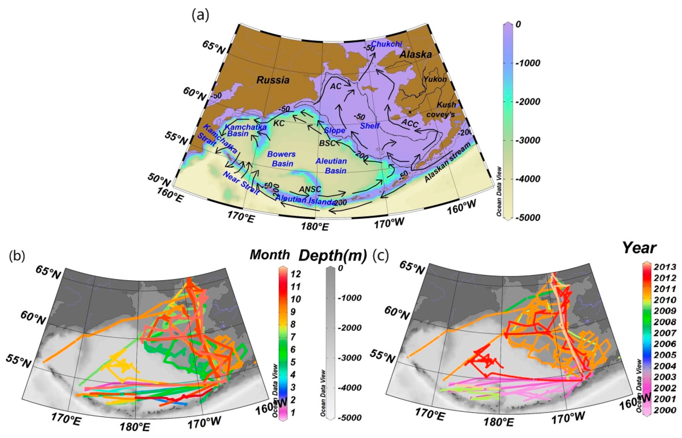
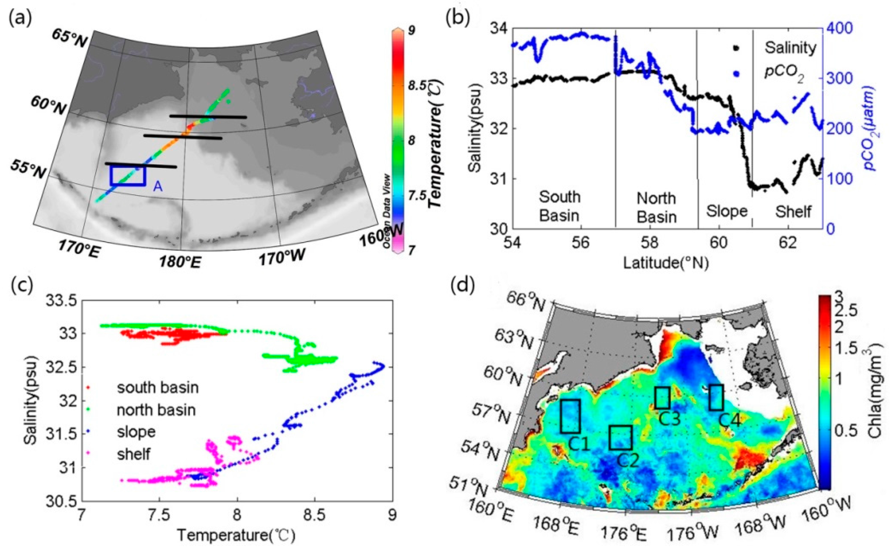
2.1. Study Area

The Bering Sea is located in the northern part of the Pacific Ocean (51–66°N and 160°E–158°W) (Figure 1a). It is bordered by Siberia in the west, Alaska in the east, and the Aleutian archipelago and the North Pacific Ocean in the south. The southwestern part of the Bering Sea is a basin (including, from east to west, the Kamchatka Basin, the Bowers Basin, and the Aleutian Basin), with depths over 3500 m in 40% of the area. The northeastern part is a shelf area with a depth of less than 200 m, whose area is about half of the Bering Sea. The shelf area has high productivity [3,4], while the basin has relatively low productivity [5].

Currents in the Bering Sea are complex (Figure 1a). Pacific water flows from east to west along the southern side of the Aleutian archipelago and merges into the Alaskan Stream, where it then enters the Bering Sea through the channels of the Aleutian archipelago. After the Alaskan Stream enters the Bering Sea, a portion of it flows northwestwards and, together with the Kamchatka Current (KC), flows southwards out of the Bering Sea along the west coast. Another portion of this water mass flows eastwards, together with the Aleutian North Slope Current (ANSC), and joins the Bering Slope Current (BSC) at ~167°W and flows northwards [34]. A portion of the BSC flows northwards to form the Anadyr Current (AC), and another portion joins the KC, flows along the west coast and then flows out of the Bering Sea through the Kamchatka Strait [35,36]. The ANSC, BSC, and KC constitute a gyre in the basin area [37]. Therefore, the Alaskan Stream has great influence on the water properties in the ANSC, southern KC, and the basins [37]. The water mass is relatively stable in the central basin due to little influence from the currents and water exchange [35]. The eastern shelf is influenced by the inputs from the Yukon River and the Kush Yanukovich River at 63°N and 60°N, respectively. Thus, the low-salinity Alaskan Coastal Current (ACC) is primarily from the mixed water mass of northeastern Pacific water and the river plumes [37,38,39].

Sea ice is a non-negligible factor for pCO₂ variability in the shelf regions of the Bering Sea, and its inter-annual variability causes different seawater properties between the south and north parts of the shelf [40]. The ice reaches the maximum in February to March, and melts from July to October [41]. The thickness, areal coverage, and southernmost extent of sea ice vary on multiple timescales [42,43,44].

Cross et al. [23] reported that the biological contribution to the carbon sink on the eastern shelf of the Bering Sea from April to December was 3.36 TgCyr⁻¹. They also found this area was a weak carbon source in autumn, but it was a sink from April to May, accounting for approximately one third of the annual carbon sink. Thus, the remaining summer flux was the greatest portion of the annual flux (~55%). In summer, there is generally an intense seasonal thermocline existing within a depth range of approximately 50–100 m (e.g., [2,45,46]); and the surface water is less influenced by vertical mixing in the basin region due to stratification, resulting in temperature and biology as the two main processes influencing pCO₂. Thus, as a first step of pCO₂-MeSAA algorithm development for the Bering Sea, we focus only on the summer season (July through September).

2.2. Data and Methods

In situ data included underway temperature, salinity, and pCO₂ in the Bering Sea during 2000–2013, downloaded from the Carbon Dioxide Information Analysis Center (CDIAC) [47]. Data distribution is most abundant from May through September (Figure 1b), and were the richest in 2010 including the data from the basin, slope and shelf areas (Figure 1c). In addition, dissolved inorganic carbon (DIC), total alkalinity (TA), and apparent oxygen utilization (AOU) in August 2004 were also obtained from CDIAC [48]. Individual cruises and data contributors are listed in

Table 1. Basic information for underway data and discrete carbonate data from CDIAC used in this research.

Cruise	Ship/Experiment	Parameters	Period of Record	Observer
M/S Alligator Hope Lines 1999–2001	M/S Alligator Hope	pCO2, Sal., temp.	January 2000 to December 2000 January, February, April, May 2001	Y. Nojiri NIES Japan
VOS Lines 2001–2006	M/V Pyxis	pCO2, Sal., temp.	July, August, November 2002 January, March 2003 May, July to October 2009 January, February, April 2013	Y. Nojiri NIES Japan
Transit	M/V Turmoil	pCO2, Sal., temp.	July 2010	/
Aleutian Is.	R/V M.G. Langseth 11/3	pCO2, Sal., temp.	July 2011, August 2011 * September to October 2011	LDEO Tech
XUE_CHINARE2010_Arctic xue_arctic08	R/V Xue Long	pCO2, Sal., temp.	July 2010 *, August 2010 September 2010 * July to September 2008	AMOL R. Wanninkhof Group
NA	NOAA Miller Freeman	pCO2, Sal., temp.	September, October 2009 September, October 2010	PMEL Feely Group
FOCI2000 FOCI2001a FOCI2001b	R/V Ron Brown 2000	pCO2, Sal., temp.	September 2000 May, June 2001	AMOL R. Wanninkhof Group
NA	R/V Thomas Thompson	pCO2, Sal., temp.	May 2010	/
NA	R/V N.B Palmer	pCO2, Sal., temp.	July, August 2003	/
Arctic Research	USCGC Healy	pCO2, Sal., temp.	June to December 2011	USCG Tech
NA	USCGC Polar Sea	pCO2, Sal., temp.	October 2013	/
MR04-04	Mirai	DIC, TA, AOU, sal., temp.	August 2004	M. Wakita S. Watanabe

pCO₂ (sea surface partial pressure of carbon dioxide); Sal. (salinity); temp. (temperature); DIC (dissolve inorganic carbon), TA (total alkalinity), AOU (apparent oxygen utilization). * Cruises in the Bering Sea basin in July 2010, August 2011 and September 2010. All other cruises were conducted on the eastern shelf.

.

The satellite data were eight-day and monthly composite MODIS/Aqua products of SST and chla, with a spatial resolution of 4 km, and were obtained from the NASA ocean color website [49]. Since the CDIAC dataset did not contain chla data, we matched the eight-day composite satellite chla with the CDIAC underway data in the same time and space windows.

Partial pressure of atmospheric CO₂ (pCO_2(air)) was calculated from the CO₂ mole fraction of dry air (xCO₂), temperature, sea surface vapor pressure (pH₂O), and sea-level total pressure (SLP) using Equations (1) and (2):

$$\mathrm{p}\mathrm{C}{\mathrm{O}}_{2(\mathrm{air})}=\mathrm{x}\mathrm{C}{\mathrm{O}}_2\times (\mathrm{SLP}-\mathrm{p}{\mathrm{H}}_2\mathrm{O})$$

(1)

$$\mathrm{p}{\mathrm{H}}_2\mathrm{O}=0.981\times {\mathrm{e}}^{(14.3262-(5306.83/(273.15+\mathrm{T})))}$$

(2)

The air-sea CO₂ flux (F) was calculated using the following equations:

$$\mathrm{F}=\mathrm{K}\times \partial \times (\mathrm{p}\mathrm{C}{\mathrm{O}}_{2(\mathrm{sea})}-\mathrm{p}\mathrm{C}{\mathrm{O}}_{2(\mathrm{air})})$$

(3)

$$\mathrm{K}=0.39\times {\mathrm{U}}_{10}^2\times {(\mathrm{Sc}/660)}^{-1/2}$$

(4)

where K is the gas exchange velocity, and U₁₀ is monthly average wind speed at 10 m; Sc is the Schmidt number [50]; ∂ is the solubility of CO₂, a function of temperature and salinity [51]; and pCO_2(sea) is the sea surface pCO₂. Since we did not aim to show the amount and distribution of air-sea CO₂ flux in this paper, we only used the traditional equation for K calculation (Equation (3)), and took the flux as one of the controlling factors on pCO₂ variation.

We also calculate DIC accumulation (∆DIC_air-sea) from winter to the summer resulting from the invasion of air-sea CO₂ flux, by using the iteration method [12]. First, we obtain the initial TA, DIC, salinity, and temperature in winter from cruise measurement and calculated the initial pCO₂ using CO2SYS (MatLab version [52,53]). Next, a new pCO₂ at the temperature in the next month is calculated with the temperature rise from March to July obtained from the climatological monthly satellite SST data. For the respective ∆pCO_{2 (air-sea)}, the air-sea CO₂ flux was calculated with Equations (3) and (4), and this amount of CO₂ for a monthly time step is then added to the DIC inventory in the mixed layer. Using the new DIC and constant TA, a new pCO₂ is calculated for the next time step, and so on. The detail value in the calculation will be discussed in Section 4.1.

The re-equilibrium time ($\tau$) triggered by the air-sea CO₂ flux can be calculated with the following equations [54,55,56]:

$$\mathsf{\tau }=\frac{\mathrm{H}}{\mathrm{K}}\times \frac{1}{\mathrm{R}}\times \frac{[{\displaystyle \sum \mathrm{C}{\mathrm{O}}_2}]}{[\mathrm{C}{\mathrm{O}}_{2(\mathrm{aq})}]}$$

(5)

$$\mathrm{R}=\frac{\Delta [\mathrm{C}{\mathrm{O}}_2]}{[\mathrm{C}{\mathrm{O}}_2]}/\frac{\Delta \mathrm{DIC}}{\mathrm{DIC}},$$

(6)

where H is the mixed layer depth; $[{\displaystyle \sum C{O}_2}]/[C{O}_{2(aq)}]$ denotes the ratio of DIC to free CO₂ in seawater, which is generally set as 100 [57]; and R is the Revelle Factor, characterizing the change in DIC caused by the change in (CO₂) in seawater and generally ranges from 8 to 15 [58,59].

For the above calculations, SLP data were obtained from the NOAA/ESRL Physical Sciences Division NCEP/NCAR Reanalysis data, with a resolution of 2.5° × 2.5° [60]. xCO₂ (ppm) data were obtained from the NOAA/ESRL Global Monitoring Division Carbontracker Project [61], with a spatial resolution of 3° × 2°. Climatological monthly average mixed layer depth data are from the website [62], with a spatial resolution of 2° × 2°. Monthly average wind speed data (WindSat data) are from the website [63], with a spatial resolution of 0.25° × 0.25°.

3. Implementation of the MeSAA Algorithm for pCO₂ in the Bering Sea

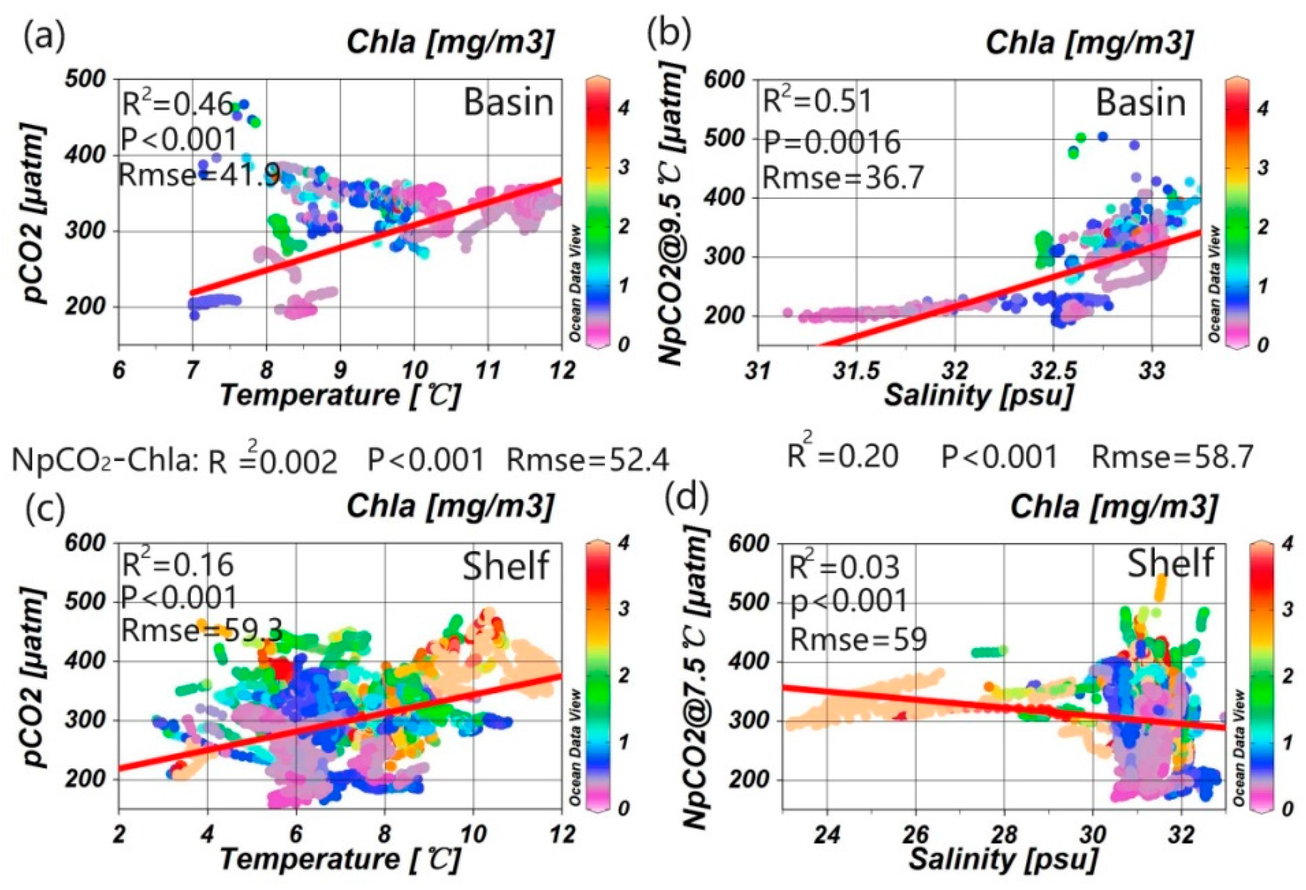
3.1. Correlations between Underway pCO₂ and Related Parameters

First, we wanted to examine the validity of simple regression methods in the Bering Sea. We analyzed the correlations between pCO₂ and temperature, salinity, and chla using all underway data from July to September. We found that pCO₂ did not show a relationship with temperature or salinity (Figure 2). In the basin pCO₂ roughly exhibited a decreasing relationship with increasing temperature (R² = 0.46) in the basin (Figure 2a), while the root-mean-square error (RMSE) in the basin was as high as 41.9 μatm. In the shelf area, relationship between pCO₂ and temperature was messy (R² = 0.16) (Figure 2c). On the whole, there was no apparent relationship between pCO₂ and temperature. pCO₂ had a weak positive relationship with salinity in the basin area (R² = 0.51, RMSE = 36.7 μatm, p = 0.0016) (Figure 2b), while there was no apparent relationship on the shelf (R² = 0.03) (Figure 2d). On the shelf, data with salinity ranging from 25 to 30 and the corresponding high chla (>2.5 mg/m³) were located in the area influenced by the Yukon River plume (167.3°W, 62.8°N). On the whole, pCO₂ did not exhibit a decreasing relationship with increasing chla as expected, with R² lower than 0.2. In summary, the relationships between these parameters were not apparent and the influences of various mechanisms on pCO₂ were variable in different areas. Thus, it was difficult to establish an empirical algorithm to retrieve pCO₂ from the temperature, salinity, and chla using regression relationships.

3.2. The MeSAA Algorithm for pCO₂

Based on the principle of the MeSAA method proposed by Bai et al. [33], sea surface pCO₂ variation (ΔpCO₂) can be expressed as the sum of individual pCO₂ contributions associated with each process or controlling factor ($\partial$pCO_2(factor-n)):

$$\begin{array}{cc}\Delta \mathrm{p}\mathrm{C}{\mathrm{O}}_2& =\left(\frac{\partial \mathrm{p}\mathrm{C}{\mathrm{O}}_{2（\mathrm{therm}）}}{\partial {\mathrm{V}}_{\mathrm{therm}}}\right)\Delta {\mathrm{V}}_{\mathrm{therm}}+\left(\frac{\partial \mathrm{p}\mathrm{C}{\mathrm{O}}_{2（\mathrm{mix}）}}{\partial {\mathrm{V}}_{\mathrm{mix}}}\right)\Delta {\mathrm{V}}_{\mathrm{mix}}+\left(\frac{\partial \mathrm{p}\mathrm{C}{\mathrm{O}}_{2（\mathrm{bio}）}}{\partial {\mathrm{V}}_{\mathrm{bio}}}\right)\Delta {\mathrm{V}}_{\mathrm{bio}}\hfill \\ & +\left(\frac{\partial \mathrm{p}\mathrm{C}{\mathrm{O}}_{2（\mathrm{air}-\mathrm{sea}）}}{\partial {\mathrm{V}}_{\mathrm{air}-\mathrm{sea}}}\right)\Delta {\mathrm{V}}_{\mathrm{air}-\mathrm{sea}}+\mathrm{....}+\left(\frac{\partial \mathrm{p}\mathrm{C}{\mathrm{O}}_{2（\mathrm{factor}-\mathrm{n}）}}{\partial {\mathrm{V}}_{\mathrm{factor}-\mathrm{n}}}\right)\Delta {\mathrm{V}}_{\mathrm{factor}-\mathrm{n}}+\mathsf{\epsilon }\hfill \end{array}$$

(7)

where ΔV_factor-n represents an individual process that varies independently of the other processes and ε is the residual error. In general, the major factors controlling pCO₂ variability are identified as: (1) the temperature-dependent thermodynamic effect (therm); (2) mixing between water masses with different values of marine carbonate parameters (mix); (3) the biological effect (bio); and (4) air-sea exchange (air-sea).

The surface water pCO₂ is linked directly to DIC, TA, and/or pH in the marine carbonate system in nonlinear relationships. The relationships among pCO₂, DIC, TA, and pH are fully mathematically defined. As DIC and TA are measured in total concentration, they are mass-conservative during mixing processes; and DIC is directly linked by stoichiometry to nutrient removal/release and O₂ production or consumption during biological processes. Thus, many studies ([33], and references therein), especially marine carbonate models, calculate pCO₂ from DIC and TA variations by estimating contributions to DIC by specific processes of mixing, biological effect and air-sea CO₂ exchange. Because our desired final product is satellite-derived DIC and TA, we chose to estimate pCO₂ directly to avoid error propagation from estimations of satellite-derived DIC and TA, even though our MeSAA approach was built upon the principle of DIC and TA changes and we also used carbonate system calculations as part of our approach. Thus, we assume ΔpCO₂ is analytically expressed as the sum of contribution from several independent processes, and the critical issue of MeSAA is how to derive the analytical expressions of each individual pCO₂ components using satellite-derived variables.

As described earlier, thermodynamics and biology are the two main factors influencing sea surface pCO₂ in the Bering Sea in summertime. Therefore, we implement the MeSAA algorithm in this paper as follows: first, we need to identify a water mass where temperature is relatively stable and pCO₂ is minimally influenced by mixing and biology; this water mass is then used as a reference (pCO_2(o)). Second, we develop parameterization methods to quantify the individual thermodynamic (ΔpCO_2(therm)) and biological effects (ΔpCO_2(bio)), and, finally, add them to pCO_2(o) as in Equation (8):

$$\mathrm{p}\mathrm{C}{\mathrm{O}}_2=\mathrm{p}\mathrm{C}{\mathrm{O}}_{2(\mathrm{o})}+(\frac{\partial \mathrm{p}\mathrm{C}{\mathrm{O}}_{2（\mathrm{therm}）}}{\partial {\mathrm{V}}_{\mathrm{therm}}})\Delta {\mathrm{V}}_{\mathrm{therm}}+(\frac{\partial \mathrm{p}\mathrm{C}{\mathrm{O}}_{2（\mathrm{bio}）}}{\partial {\mathrm{V}}_{\mathrm{bio}}})\Delta {\mathrm{V}}_{\mathrm{bio}}$$

(8)

3.2.1. Reference Water Mass and Temperature Effect

Since the July 2010 cruise was the only cruise that passed through the basin, slope, and shelf areas (Figure 3a), we used this dataset to analyze the properties of the water masses in different regions, in order to determine the reference water mass and the pCO_2(o) term. We divided the different regions into four zones along the cruise track according to latitudinal distribution of underway salinity and pCO₂ features (Figure 3b). Region 1: in the southern part of the basin (54–57°N), the water masses were relatively stable, and pCO₂ (367.5 ± 18.0 μatm), salinity (32.98 ± 0.06), and temperature (7.57 ± 0.16 °C) varied very little with latitude. Region 2: in the northern part of the basin (57–59.5°N), pCO₂ decreased with decreasing salinity and also was negatively related to temperature. The water in the northern basin might be influenced by mixing with the northwestwards flowing BSC with relatively low salinity and low pCO₂. Region 3: in the slope area (59.5–61°N), salinity, and pCO₂ reached their minima due to high biological production. According to Springer et al. [3], the area near 61°N was located in the “Bering Sea Green Belt”. This area was at the shelf-slope front, and the shelf–basin exchange processes, such as tidal mixing and eddies, provided high nutrient concentrations to the surface layer, resulting in primary production here up to 175–275 gCm⁻²·y⁻¹, 60% higher than that in the adjacent shelf area. Region 4: in the shelf area (above 61°N), salinity and pCO₂ increased slightly compared with the slope area, however, pCO₂ was still relatively low (below 280 μatm) compared with the other regions. In this region we also found that there was a weak positive relationship between pCO₂ and salinity, which might be influenced by mixing with the northwards flowing BSC.

The water mass in the southern basin was relatively stable as suggested by in situ pCO₂, salinity, and temperature variability; chla was at a relative low level (below 0.5 mg/m³) compared with other areas, seen from the climatological average (2002–2014) satellite chla image in July (Figure 3d in box C2). Therefore, we selected the water mass in the southern basin as the reference water mass (55.7–57°N, 171.4–174.2°W), shown in box A of Figure 3a. In a total of 238 sets of data, temperature (7.7 ± 0.1 °C) and salinity (32.98 ± 0.02) in the selected reference water changed very little (Figure 3c), indicating the limited influence of water mixing. Furthermore, the average temperature of the reference water mass (7.7 ± 0.1 °C) was within the temperature range (6 to 12 °C) of the basin and slope areas in summer, thus errors resulting from the wide temperature range of pCO₂ normalization by the thermodynamic equation should be minimal [33,64]. We also calculated the monthly composite MODIS/Aqua SST during 2002–2014 within this area, and its average standard deviation (SD) for individual months during these 13 years was within ± 0.9 °C, indicating a small inter-annual change in temperature. Overall, the selected water mass was relatively stable and could be used as a reference water mass for the remote sensing algorithm of pCO₂.

The temperature-dependent thermodynamic effect on sea surface pCO₂ has an exponential relationship of approximately 4.23%/°C [21,59,65]. Note that the slope of 0.0423 was derived for the global ocean, and this can be confirmed with carbonate system calculations, although the slope varied slightly with TA, DIC, salinity and temperature [33]. Thus, we can analytically calculate the pCO₂ at a certain temperature (T) by the exponential relationship as in Equation (9) [21,59,65]. Note that pCO_2(T) in Equation (9) represents the first two items in the Equation (8), which combined the value of reference water (pCO_2(o)) and the temperature-dependent thermodynamic effect.

$$pC{O}_{2(\mathrm{T})}=pC{O}_{2(O)}\times \exp (0.0423\times (T-T_{(O)}))$$

(9)

Briefly, we used the average values in the reference water mass as pCO_2(o) = 381.8 ± 5.1 and temperature T_(o) = 7.7 ± 0.1 (

Table 2. Values for the different parameters in the reference water mass and water in the minimum temperature layer in the summer. Data in the parentheses are the standard deviation from the average values of N = 238 data points.

Title	Location	Temperature (°C)	Salinity (psu)	pCO2	DIC μmol/kg	TA μmol/kg	AOU μmol/kg
Reference water a	55.7–57°N 171.4–174.2°W	7.70 (0.11)	32.98 (0.02)	381.80 (5.08)	/	/	/
Station 38 b	57°N 172.5°E	2.42 °C	33.25	/	2154.40	2239.70	35.98
Calculated winter data c	/	2.42 °C	33.25	415.10	2126.76	2239.70	/

^a The values of the reference water in the basin from July 2010 (Box A in Figure 3). ^b The value of the temperature minimum layer at a depth of 100 m from August 2004. ^c The values of well-mixed winter water, calculated from the summer data in the temperature minimum layer (Station 38); see the text for detail.

), as well as the temperature effect on pCO₂ under a constant TA, DIC, and salinity [65]. pCO_2(o) was an empirical value in practice, and we will prove its stability through further marine carbonate system analysis in Section 4.1.

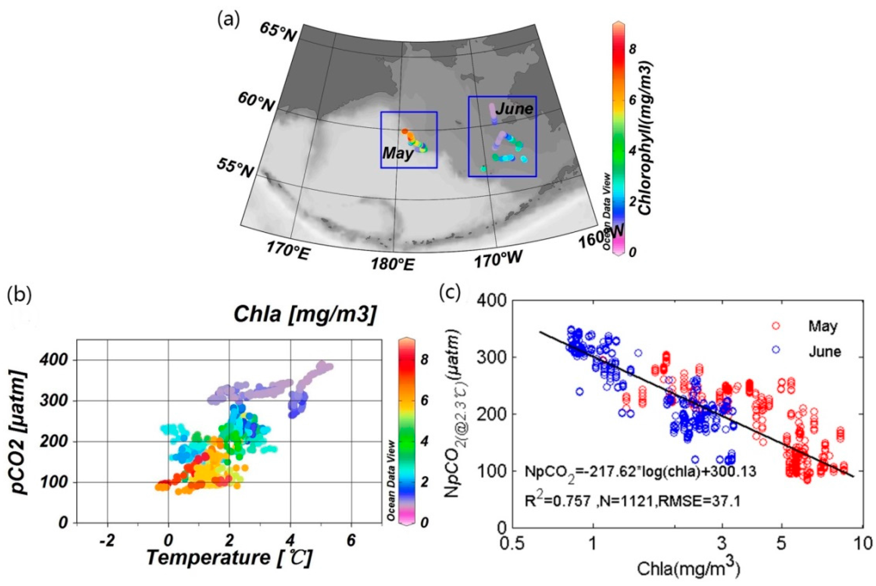
3.2.2. Quantification of Biological Effect

The biological effect on pCO₂ variability is an indirect and complex process that changes the DIC concentration through various processes, such as photosynthesis/respiration and/or CaCO₃ production/dissolution, and thus changes pCO₂. Direct and accurate analytic expressions of these processes are still an open question [27,64]. For practical satellite data processing we used a similar method to that in Bai et al. [33], which uses an integral to express pCO₂ drawdown with an increase of chla. In an area mainly controlled by biological activities, it can be assumed that pCO₂ and chla have the following relationship [33]:

$$\mathrm{p}\mathrm{C}{\mathrm{O}}_2=\mathrm{A}-\mathrm{B}\times \log (\mathrm{chla})+\mathsf{\epsilon },$$

(10)

where $\epsilon$ represents the contribution from other factors independent of biological effects. The influence of the biological effect on pCO₂ exhibits an accumulation effect with time, so the ΔpCO_2(bio) can be expressed with the following equation [33]:

$$\begin{array}{cc}\Delta pC{O}_{2(bio)}& =\frac{\partial pC{O}_{2（bio）}}{\partial V_{bio}}\Delta V_{bio}={\displaystyle {\int }_{chl{a}_0}^{chl{a}_n}-\frac{B}{\ln (10)}\frac{1}{chla}d(chla)}\hfill \\ & =-\frac{B}{\ln (10)}\times [\ln (chl{a}_n)-\ln (chl{a}_0)]\hfill \end{array},$$

(11)

where Chla_n is the sea surface chlorophyll concentration, and Chla₀ is the background value.

A subset of data controlled mainly by the biological effect, with little influence by terrestrial input and mixing effect, needed to be determined to regress the coefficient B in Equation (10). Due of not having in situ chla data and few available chla data in the daily satellite products due to cloud cover, we matched the eight-day composite satellite chla data with underway data. Through analyzing all available match-up data in the spring and summer, we found that pCO₂ and chla had significant negative relationships during May to June 2010, which were located on slope and shelf areas (Figure 4a,b); therefore, we used this subset of data for further analysis. The thermodynamic effect should first be eliminated in order to remove this apparent effect when analyzing the other processes. We normalized pCO₂ (NpCO₂) to the average temperature (2.3 °C) of this subset (Figure 4c). There was a significant negative relationship between NpCO₂ and chla with R² = 0.757 (Figure 4c); furthermore, the consistent relationship in May and June indicated that pCO₂ drawdown caused by per chla production was relatively consistent in this area. Thus, we obtained the coefficient B in Equation (10) as:

$$\mathrm{N}\mathrm{p}\mathrm{C}{\mathrm{O}}_2=-217.62\times \log (\mathrm{chla})+300.13.$$

(12)

Consequently, pCO₂ variability caused by the biological effect can be expressed as Equation (13). The chla₀ in Equation (11) was taken empirically as 0.1 mg/m³, according to the generally low chla level in the basin area.

$$\Delta \mathrm{p}\mathrm{C}{\mathrm{O}}_{2（\mathrm{bio}）}={\displaystyle {\int }_{{\mathrm{chla}}_0}^{{\mathrm{chla}}_{\mathrm{n}}}-\frac{\mathrm{B}}{\ln (10)}}\frac{1}{\mathrm{chla}}\mathrm{d}(\mathrm{chla})=-217.62\times [\log ({\mathrm{chla}}_{\mathrm{n}})-\log (0.1)]$$

(13)

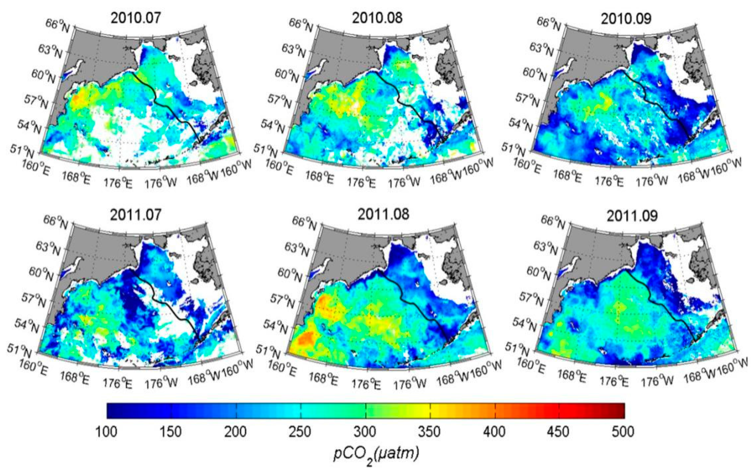
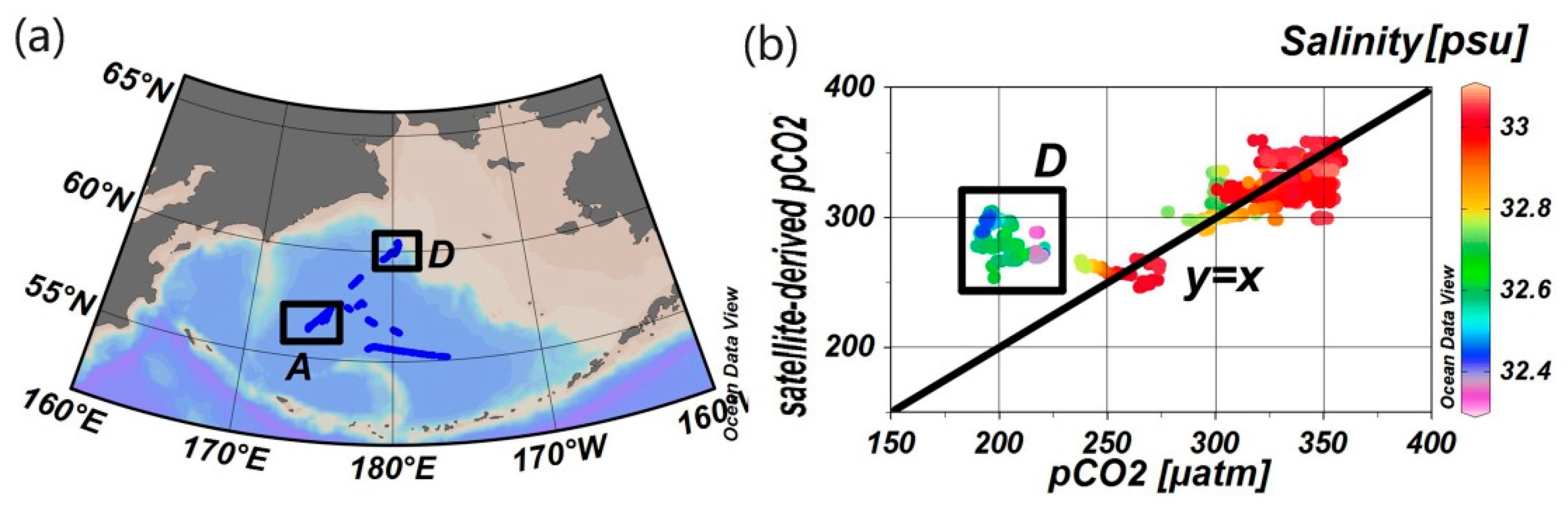
3.3. Results and Validation

We generated monthly composite satellite SST and chla data for July, August, and September of 2010 and 2011 based on the inversion models (Equations (8), (9), and (13)). The accuracy of satellite-derived chla might be not good at the Bering Sea, and showed systematic overestimation for the SeaWiFS OC4V4 algorithm (i.e., [66,67]). The ocean optical community must improve the chla algorithm in some special sea, like the Bering Sea. However, such systematic deviation of satellite-derived chla had been eliminated from the pCO₂-MeSAA algorithm development. Because of not having in situ chla data, we matched the MODIS-derived chla data with underway pCO₂ data. Through the regression, we get the key coefficient of ∂(pCO2@bio)/∂(log(chla)) and finally, calculate the pCO₂ drawdown caused by phytoplankton carbon uptake with MODIS-derived chla (Equation (13)). In these procedures, the systematic deviation has less influence on the estimated pCO₂ in MeSAA algorithm.

From the images of satellite-derived pCO₂ (Figure 5), pCO₂ in the basin was approximately 250–360 μatm, and lower than atmospheric pCO₂ (387 μatm) in most of the Bering Sea. pCO₂ on the slope was lower than that in the basin, ranging from 200 to 300 μatm; and pCO₂ in the shelf area ranged from 100 to 250 μatm. pCO₂ varied both spatially and temporally over the Bering Sea during the years studied. Due to high SST in August (10.38 ± 0.29 °C in 2010 and 10.48 ± 0.36 °C in 2011) pCO₂ was generally higher in August (241.3 ± 13.1 μatm in 2010 and 252.8 ± 14.1 μatm in 2011) than in July and September, especially in the basin area with low chla. High chla concentration in the slope and shelf areas, as well as some patchiness of algal blooms in the basin, resulted in under-saturated pCO₂ with respective to the atmosphere, with pCO₂ as low as ~100 μatm.

For validation of satellite-derived pCO₂, we matched up satellite data with underway measurements, and narrowed the temporal and spatial gap between these two datasets as much as possible. However, the MODIS/Aqua data (a spatial resolution of 4 km) had few available data in daily products due to the heavy cloud coverage. Therefore, we used the eight-day composite satellite data. There were only three cruises from July to September in our datasets—July 2010, August 2011, and September 2010—and the available data matched up primarily in the central basin and near the slope region (Figure 6a). Since the data in the central basin from July 2010 had been used to calculate the reference values (Box A in Figure 3a and Figure 6a), we exclude this data in the validation in Figure 6b. In general, satellite-derived pCO₂ was consistent with the underway pCO₂, especially in the basin (Figure 6b). The RMSE for the entire validation data set in eight-day composite MODIS was 9.87% (N = 1274, SD = 35.11 μatm). For the central basin, the average RMSE was 4.37%, ranging from 0.04% to 14.95% (N = 1052, SD = 17.67 μatm). For the slope, the average RMSE was 35.9%, ranging from 22.81% to 55.61% (N = 222, SD = 74.8 μatm), and the satellite-derived pCO₂ was about 50 μatm higher than the underway pCO₂ (data in box D in Figure 6b, in which salinity was below 32.7). This is an interesting phenomenon and will be discussed in Section 4.2.

In order to check the validation on a larger scale, we also used the monthly-composite satellite data, and compared the results with underway data in general trends (Figure 7). The MeSAA prediction yielded the best consistency with data in the basin area (Figure 7d), as well as the offshore area near the west coast of the Bering Sea (Figure 7b). The data used for validation were independent of those used to develop the algorithm, thus the current comparisons have proved good reliability of MeSAA algorithm in the majority of the Bering Sea. In the shelf area, the satellite-derived pCO₂ near the 50 m isobaths was, however, significantly underestimated (Figure 7c). Un-predicted high pCO₂ in the shelf area might be a result of two possibilities: (1) the influence of the Yukon and Kush Yanukovich River plumes, where in situ pCO₂ was up to ~390 μatm due to the re-mineralization of terrestrial organic matter; and (2) the effect of coccolithophorid blooms. We will discuss these in Section 4.2.

In summary, the data we used to validate the satellite-derived pCO₂ were totally independent data that had not been used in the algorithm development. Comparison results showed good agreement between satellite-derived pCO₂ and underway data, especially in the central basin. With the mechanistic principle of MeSAA algorithm, the deviation between the satellite results and in situ data can highlight unconsidered processes; such deviations help to further understand the mechanism and parameterization of new components that influence pCO₂ variability. Analysis of these issues will be presented in Section 4.2 and Section 4.3.

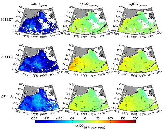
3.4. Contribution of Different Controlling Factors to the Variation of pCO₂

Since the principle of MeSAA algorithm was the sum of individual pCO₂ variations associated with each process, we could identify the contribution of different controlling factors:

$$\mathrm{N}\mathrm{p}\mathrm{C}{\mathrm{O}}_{2(\mathrm{sea})}=\mathrm{p}\mathrm{C}{\mathrm{O}}_{2(\mathrm{sea})@{\mathrm{T}}_{\mathrm{obs}}}*{\mathrm{e}}^{(0.0423*(\mathrm{T}(\mathrm{o})-{\mathrm{T}}_{\mathrm{obs}}))}$$

(14)

$$\Delta \mathrm{p}\mathrm{C}{\mathrm{O}}_{2(\mathrm{therm})}=\Delta \mathrm{p}\mathrm{C}{\mathrm{O}}_{2(\mathrm{sea}-\mathrm{air})}-\mathrm{N}\Delta \mathrm{p}\mathrm{C}{\mathrm{O}}_{2(\mathrm{sea}-\mathrm{air})}=(\mathrm{p}\mathrm{C}{\mathrm{O}}_{2(\mathrm{sea})}-\mathrm{p}\mathrm{C}{\mathrm{O}}_{2(\mathrm{air})})-(\mathrm{N}\mathrm{p}\mathrm{C}{\mathrm{O}}_{2(\mathrm{sea})}-\mathrm{p}\mathrm{C}{\mathrm{O}}_{2(\mathrm{air})})$$

(15)

$$B^{*}=N\Delta pC{O}_{2(sea-air)}=NpC{O}_{2(sea)}-pC{O}_{2(air)}$$

(16)

$$\Delta pC{O}_{2(other)}=B^{*}-\Delta pC{O}_{2(bio)}.$$

(17)

To distinguish the temperature effect from the biological effect, Cross et al. [23] normalized pCO₂ (NpCO₂) obtained in the eastern Bering Sea shelf from April to December during 2008–2012 to the annual average temperature (Equation (14)). This calculation removes the localized effects of warming and cooling on pCO_2(sea), such that the temperature effect at any one time relative to the annual average can be estimated as the difference between pCO_2(sea) and NpCO_2(sea) (Equation (15)) [23]. Accordingly, NpCO_2(sea) variability should be the result of any additional process that modifies pCO_2(sea) other than thermodynamic effects, such as biological CO₂ uptake, air–sea exchange, and vertical/lateral transport of carbon [23]. To simplify the calculation, Takahashi et al. [58], Bates et al. [1], and Cross et al. [23] all regarded the variations in NpCO_2(sea) as the result of biogeochemical effect (defined as B* in Equation (16)), which includes the other processes. For our MeSAA algorithms, however, we can quantify the contribution of biological uptake separately (Equation (13)), so the contribution of other processes (∆pCO_2(other)) can be further separated from B^* (Equation (17)).

Thus, using Equations (13)–(17), we obtained influences of three types of processes that affected pCO₂: ΔpCO_2(therm), ΔpCO_2(bio), and ∆pCO_2(other), in the Bering Sea during the summer with satellite data (shown in Figure 8). Here, we used the reference temperature T₍₀₎ = 7.7 °C in Equation (14). From July to September, ΔpCO_2(bio) was the primary influence on pCO₂, and decreased it 100–200 μatm; while the contributions of ΔpCO_2(therm) and ΔpCO_2(other) were relatively low, each about ±50 μatm. As the sea surface pCO₂ was generally lower than the atmospheric pCO₂ in summer, there was an atmospheric CO₂ influx into the surface ocean that increased pCO₂. In addition, vertical mixing also increased the ocean pCO₂ due to high DIC water from the bottom layer; therefore, ΔpCO_2(other) were generally positive, with a value of 0 to 30 μatm in most of the Bering Sea.

The ΔpCO_2(bio) pattern was neither spatially nor temporally uniform in the Bering Sea (Figure 8). Relatively low ΔpCO_2(bio) (−50–−100 μatm) in the central basin corresponded to relatively low chla (0.6 mg/m³) (Figure 3d and Figure 8). ΔpCO_2(therm) declined gradually from west to east (Figure 8), which followed the same pattern as SST. ΔpCO_2(therm) and ΔpCO_2(other) in the majority of the Bering Sea was close to equilibrium, with a slight decrease from the southwest to the northeast, especially on the shelf, except in the Kamchatka Basin.

ΔpCO_2(therm) was remarkably high in the Kamchatka Basin in the west of the Bering Sea (on the west of 170°E), reaching 60 μatm in August 2011; both chla (~0.9 mg/m³) and SST (~11.5 °C) in the Kamchatka Basin were higher than the central basin, therefore the contributions of ΔpCO_2(bio) and ΔpCO_2(therm) here were larger than in the other sub-regions; however the influence of these two effects was opposite and thus compensated for each other. Thus, the contribution of ΔpCO_2(other) was positive, but close to neutral. ΔpCO_2(other) was greater in the Kamchatka Basin than in the other sub-regions. The complex currents in the Kamchatka Basin, with the Kamchatka Current flowing out through the Kamchatka Strait, Pacific water flowing in through the Near Strait, and anticyclone eddies [35,37], cause high sea surface pCO₂ variability. In general, the contribution of the biological effect in the summer on sea surface pCO₂ variability was roughly more than twice as important as the temperature effect. Other processes increased the sea surface pCO₂ but their influences were similar to, or slightly less than, the influence of the temperature effect.

4. Discussion

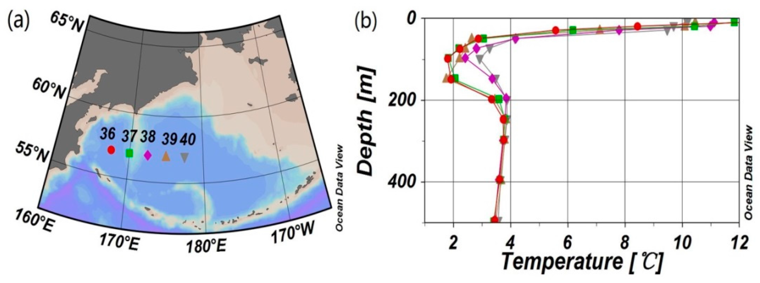
4.1. Stability of Reference Water Mass

The reference water mass for the MeSAA model in the Bering Sea was chosen in the central basin, where currents and mixing had a minimal influence on sea surface pCO₂. The location of the reference water mass was close to the entrance of the Alaskan Stream flowing into the Bering Sea from the Near Strait. Thus, the stability of the reference water mass would be influenced by the Alaskan Stream water properties and flow rate. Favorite [68] suggested that the flow rate of the Alaskan Stream from the Near Strait was constant (10 × 10⁶ m³·s⁻¹). Onishi et al. [69] also found that the Alaskan Stream was stable, with relatively high homogeneity in the vertical direction compared with the surrounding water masses [70]. Therefore, we assume that the variation of the Alaskan Stream had little influence on the properties of the reference water mass.

Next we discuss carbonate system variability of the reference water mass for its source and seasonal evolution (Equations (18) and (19)). In MeSAA algorithms, our defined reference pCO_2(o) in summer could be regarded as the result of well-mixed winter water (pCO_2(winter)) going through a series of processes, such as warming, biological alteration (∆pCO_2(bio)), and air-sea exchange (∆pCO_2(air-sea)), to evolve into the summer status (pCO_2(summer)) (Equation (18)). We now try to quantify this seasonal evolution using marine carbonate system calculations; the comparison between selected pCO_2(o) and calculated pCO_2(summer) can check the stability of reference water mass. TA is assumed to be constant in this area based on the stable Alaskan Stream and limited influence from currents mixing in the central basin, thus variations in pCO₂ will depend on DIC change (Equation (19)).

$$pC{O}_{2(summer)}=pC{O}_{2(w\mathrm{int}er)}-\Delta pC{O}_{2(bio)}-\Delta pC{O}_{2(air-sea)}$$

(18)

$$\begin{array}{cc}DI{C}_{(summer@surface)}& =DI{C}_{(w\mathrm{int}er@surface)}-\Delta DI{C}_{air-sea}\hfill \\ & =[DI{C}_{(summer@temp-\min -layer)}-\Delta DI{C}_{bio}]-\Delta DI{C}_{air-sea}\hfill \end{array}$$

(19)

First we determined DIC and TA values in winter surface water based on field measurements. In order to avoid differences between cruises, we estimated winter values from summer observations. We were able to do this as there was a temperature minimum layer (below 3 °C) at 75–150 m in summer under the thermocline in the Bering Sea basin; this layer was regarded as a remnant of the winter surface layer [45,46,71,72]. Therefore, we used observations from the temperature minimum layer in summer as winter values; however, it should be pointed out that these values still include biologically produced DIC (∆DIC_bio), which should be removed to obtain a final winter value (Equation (19)). In the spring and summer, the organic carbon produced by the phytoplankton photosynthesis in the upper layer sinks to the lower layer, and is decomposed into inorganic carbon through biological respiration (∆DIC_bio). This process was recorded by the apparent oxygen utilization (AOU), and could be converted to carbon concentration based on the Redfield Ratio [73] (ΔDIC_bio = 106*AOU/138). There was only one set of inorganic carbon observations obtained during the summer in the PACIFICA database: data from an east-to-west section at 57 °N in August 2004 (Figure 9a). The minimum temperature (2–3 °C) occurred at the depth of 100 m at all stations during this cruise (Figure 9b), indicating that the properties of the water mass in this area were constant and stable. We used data from Station 38 (Table 2), which was closest to the position of our selected reference water mass. As AOU = 35.98 μmol/kg in the temperature minimum layer, we obtained ΔDIC_bio = 106*AOU/138 = 27.7 μmol/kg, thus the well-mixed winter DIC value was 2126.76 μmol/kg (Station 38 summer value minus ΔDIC_bio). With the unchanged TA, pCO_2(winter) was calculated to be 415.1 μatm. Since sea surface pCO₂ in the winter was higher than atmospheric pCO₂ (387.2 μatm), CO₂ would have outgassed to the atmosphere. Thus, ∆DIC_air-sea from winter to summer (set as March to July) could be calculated with the iteration method (see the description in Section 2.2), and the relative values in the iteration calculation were as follows. The initial conditions including the DIC, TA, temperature, and salinity were set as those in March (winter value) (Table 2); we assumed that the wind speed was constant as the average value during March to July (7.28 m/s from climatologic satellite data) and the temperature raising rate in surface seawater was constant at 0.035 °C/d [(T₀-T_winter)/150]. The climatological monthly average mixing layer depth was 50.7 m during March to July (Section 2.2). We assume an atmospheric pCO₂ of 387.2 μatm from the average xCO₂ data during March to July (Equations (1) and (2)). After the iteration calculation from March to July (150 days), we obtained the final ∆DIC_air-sea as 20.36 μmol/kg. If there were only air–sea exchange and warming effects on the surface water, the surface DIC in summer decreased to 2106.4 μmol/kg according the T_(o) = 7.7 °C in July (Equation (19)), and then the calculated pCO_2(summer) was 450.9 μatm. Considering that chla in the reference water mass was approximately 0.2 mg/m³ in July 2010, ∆pCO_2bio was estimated with Equation (13) to be 65 μatm, then the final pCO_2(summer) was 385.9 μatm.

In summary, starting with a pCO₂ in winter of 415.1 μatm, and after a series of processes as air-sea exchange and warming (increase by 35.8 μatm)) and biological effect (decrease by 65 μatm), pCO_2(summer) was about 385.9 μatm. This calculated summer value was close to the reference pCO_2(o) (381.8 μatm).

The above calculation used a traditional Redfield C:O ratio of 106:139 [73]. Considering the Redfield ratio is various over different biogeochemical conditions (e.g., [74,75,76,77]), we used C:O ratios ranging between 94:131.8 and 134:162 [77] to test its sensitivity. Then, we obtained the calculated well-mixed winter DIC value as 2124.64–2128.74 μmol/kg. With the unchanged TA, pCO_2(winter) was calculated to be 408.7–421.3 μatm. The surface DIC in summer decreased to 2105.7–2106.9 μmol/kg according the T_(o) = 7.7 °C in July (Equation (19)), and finally the calculated pCO_2(summer) was 448.7–452.4 μatm. The result (448.7–452.4 μatm) considering the Redfield ratio variability was very close to that with the traditional Redfield ratio (450.9 μatm). In the central basin, since the biological level was very slow, ΔDIC_bio was also small, thus the variability in Redfield ratio had little influence on the results.

This agreement further suggests that our selected reference water mass is derived from well-mixed winter water and can be traced with quantitative processes, and thus the reference values were applicable to estimated satellite-derived sea surface pCO₂ in a long time series. The above estimation is based on simplified processes and is an approximate estimation of changes in carbonate system biogeochemistry. Future work is needed on larger scale satellite data to use the MeSAA algorithm during an entire calendar year.

4.2. Influence of the Biological Effect on pCO₂

Chla alone may not be a precise measure of, or adequate proxy for, biological processes on pCO₂, as its association with carbon uptake is variable and does not include respiration. However, satellite chla data is very practical in algorithm development and data processing [26,33]. During the phytoplankton growth phase, decreasing pCO₂ can be observed with increasing chla, which is considered in MeSAA algorithm. Thus, the biological effect was quantified as the amount of pCO₂ drawdown by per 1 mg/m³ log(cha) consumed with fitting the slope (B = −217.62) of NpCO₂ and chla. The coefficient B was higher in the Bering Sea in absolute value than that in the East China Sea (−117.5) [33]. The level of phytoplankton biomass (chla) in the Bering Sea basin was much lower than that in the East China Sea (chla = 1–4 mg·m⁻³) [78]; however, the efficiency of carbon uptake by per unit log(cha) in the Bering Sea was greater [33]. That means, for the low chla regime, dominated by small size of phytoplankton communities (pico-chla), a small increase of chla can draw down a more significant amount of pCO₂ than that in the high chla regime, which is dominated by the larger cell sized phytoplankton (micro-chla). It might be caused by a lower package effect by the smaller sized phytoplankton for photon utilization during photosynthesis, as compared to the large sized species. Similarly, Bricaud et al. [79], based on a large global in situ dataset, reported that chla-specific absorption coefficients also showed an exponential decay relationship with log(chla) due to the package effect. For a more analytical explanation, future work should focus on studying the carbon uptake efficiency by different species, and their net community productivity.

The degradation phase of the phytoplankton bloom is another aspect of the MeSAA algorithms. Different pCO₂ controlling mechanisms act on different time scales. For example, phytoplankton blooms disappear rapidly, indicated by very low chla, when nutrients are exhausted; however, both DIC and pCO₂ need to take a longer time to return to their pre-bloom status (higher concentrations), thus low-pCO₂ could still be found with low-chla [33]. This would influence the performance of current MeSAA algorithm by overestimating pCO₂. To further investigate this issue, we used time-series satellite chla data to analyze the influence of spring phytoplankton bloom on the summer pCO₂ (Figure 10). On the whole, the spring bloom peaks occurred in all areas but the timing (onset, duration, etc.) varied; however, before and after the peak chla remained at a relatively low level (Figure 10a). The spring phytoplankton bloom occurred earlier on the shelf than in the other regions, with chla reaching its peak in April (2.9 mg/m³); then on the slope with the peak occurring in May (3.02 mg/m³); and finally, in the basin when chla reached its peak in June (0.81 mg/m³).

Since sea surface pCO₂ had been drawn down to a very low level at the end of algal blooms, we could estimate the re-equilibrium time ($\tau$) of CO₂ (Equations (5) and (6) in Section 2.2), which was triggered by the large gradient of air-sea pCO₂. In the basin the biological effect was at a relatively low level and the algal bloom from April to June was not significant, therefore having little influence on pCO₂ in the summer. On the shelf the calculated re-equilibrium time ($\tau$) was roughly 40–60 days, calculated with the climatological monthly mixed layer depth from March to June of 15–20 m. The spring bloom occurred in April on the shelf but in June the chla decreased to a relatively small value; then, after a period of 1–2 months, the air–sea exchange compensated for the biological signal and re-established the air–sea equilibrium in July. Therefore, the influence of the spring bloom on the satellite-derived pCO₂ on the shelf was minimal. The adequate re-equilibrium time by air–sea exchange in the central basin and on the shelf could explain the good performance of MeSAA algorithms in these regions (Figure 7).

In contrast to the other regions, slope chla reached its peak in May and still maintained a high level (2.3 mg/m³) in June, and then decreased to 0.35 mg/m³ in July (Figure 10a). Therefore, only one month was not enough for the re-equilibrium by air–sea exchange, and pCO₂ in July still maintained a relatively low value, leading to a typical low chla and low pCO₂ phenomenon. Such a delayed influence of the previous spring’s biological effect could be a reason for the ~50 μatm overestimation of satellite-derived pCO₂ on the slope in July 2010 (Figure 6b). Another possible reason for the overestimation could be due to tidal mixing and upwelling on the slope [80,81,82]; however, these overestimated data had salinity lower than 32.7 (Figure 6b), which would be less possible from the influence of the sub-surface high-pCO₂, high salinity (>33 psu) water [46,81,83].

Specific phytoplankton functional groups that affect carbonate chemistry would also influence the pCO₂. For example, coccolithophorid blooms have been found to frequently occur on the eastern shelf of the Bering Sea from August to October [84,85,86,87,88,89]; during the blooms, the cells release CO₂ during calcification, consequently elevating the surface seawater pCO₂ [88,89]. This process offsets the DIC consumption by photosynthesis. On the shelf, we found NpCO₂ (normalized to the reference temperature of 7.7 °C) and chla had a good positive correlation (Figure 11a) Meanwhile, the deviation between the satellite-derived pCO₂ and in situ data also had a significant negative correlation with chla; it also indicated that the contributions of other processes (not considered here) on pCO₂ would be relative to the biological effects (Figure 11b) Thus, we hypothesize that the other processes not considered might be influenced by coccolithophorid blooms, which could explain the underestimation in MeSAA validation in Figure 7c. Another possibility is the influence of the re-mineralization of terrestrial organic matter, which could result in a pCO₂ increase. We infer this influence from terrestrial sources because (1) the underestimated data corresponded with low salinity (below 31 salinity units in the sub-regions in Figure 7a); and (2) the deviation between the satellite-derived pCO₂ and in situ data also showed a positive relationship with salinity below 31 (Figure 11c). Unfortunately, we do not have the necessary data to clarify these two speculations at this time. Further efforts should be made to understand the complex biological and terrestrial effect on pCO₂, and to obtain more information from the satellite data beyond chla, such as the identification of special functional groups and the timing of algal blooms (onset, duration, etc.).

4.3. The Influence of Mixing

As a first step toward implementing pCO₂-MeSAA for the Bering Sea, we chose the summer season to eliminate the influence of vertical mixing caused by the seasonal cooling; however, mixing still occurs during the summer in some areas of the Bering Sea. The main currents in the Bering Sea include the westwards flowing ANSC along with the Aleutian archipelago and the anticlockwise flowing BSC in the slope [34,35]. Seasonal upwelling, caused by wind and eddies (due to the difference of currents velocity), on the southeastern slope and southern Bering Sea close to the Aleutian archipelago, would also occur during the summer (e.g., [2,46,80,90,91]) and bring high DIC and nutrient concentrations from subsurface water to the surface layer [24]. The slope in the northeast was influenced by the broad, northwestwards flowing BSC and appeared to be a system of eddies rather than a continuous current [80,82], therefore the shelf–basin exchange processes of intensive tidal mixing and eddies likely play an important role in pCO₂ variability. Mixing processes supply nutrients to the regions adjacent to the slope and enhance primary production, eventually leading to a biological drawdown of pCO₂ [22]. The shelf was affected by mixing with the Yukon River and Kush Yanukovich River plumes increasing pCO₂ from organic carbon re-mineralization.

In this preliminary study we analyzed underway data in the central basin to access the influence of mixing on pCO₂. There were only two cruises in July 2010 and August 2011 that measured pCO₂ in the central basin during summer months. Since most of the corresponding satellite chla data in July 2010 were not available due to the cloud cover, we were limited to using only the data from August 2011 for analysis.

We divided the central basin into three sub-areas, i.e., E1, E2, and E3 (Figure 12), because the underway data covered a vast spatial scale. The three different regions were defined using scatter plots of pCO₂, temperature, and salinity. The relationship between pCO₂ and salinity showed that pCO₂ was influenced by water mixing in all three sub-areas (Figure 12b–d), in particular the sub-area E2 near the slope where temperature and salinity both showed a good positive relationship with pCO₂; this may be due to mixing of the westwards flowing branch of the BSC with the relatively low-temperature, low-salinity, and low-pCO₂ water from the branch of the westwards-flowing BSC [81]. The difference between satellite-derived pCO₂ and the underway pCO₂ had some negative relationship with the in situ salinity in several of the sub-regions (Figure 12e–g), indicating the possibility to parameterize mixing using salinity data and adding this term in the MeSAA algorithm. However, the data from August 2011 in Figure 12 were also used to validate the satellite-derived pCO₂ (Figure 6 and Figure 7); and the good agreement between the satellite results and the in situ data showed that horizontal mixing had a limited influence on sea surface pCO₂ in summer.

Developing an adequate method for parameterizing the mixing effect is an ongoing process. We suggest that future work could focus on satellite salinity data, such as the Soil Moisture and Ocean Salinity (SMOS) and Aquarius/SAC-D satellites, as a proxy for mixing, or wind-driven upwelling could be parameterized by the satellite wind data. In the coastal area, the satellite-derived CDOM is a good proxy to give additional information of shelf water and the open sea (e.g., [92,93,94]). The CDOM behaves conservatively and has good negative correlations with salinity in many large river estuaries and plume systems where physical mixing prevails, thus CDOM can be a mixing indictor in river-plume dominated coastal oceans (e.g., [93,94]). We have used the satellite-derived CDOM as one of the inputs for pCO₂ algorithm in the Changjiang River-dominated East China Sea in our previous manuscript [33]. The whole Bering Sea is not significantly influenced by large rivers (except in some northeastern inshoreareas), and the majority is basin. Actually, the controlling factors on pCO₂ variation are very complicated and the available data of multiple parameters are lacking in coastal areas, such as the localized relationship between CDOM and salinity, and the mixing behaviors of carbonate parameters, e.g., DIC and TA. Refining the methods for quantifying mixing processes in different sub-regions is needed as more data become available.

5. Conclusions

In this paper remote sensing inversion of the sea surface pCO₂ in the Bering Sea in summer was achieved with the satellite temperature and chlorophyll data using the MeSAA algorithm. The MeSAA algorithm was used to parameterize the individual effect of various factors that influence the variability of sea surface pCO₂ using a mechanistic analysis. First, a reference water mass with pCO₂ variability minimally influenced by mixing and biology was identified in the central basin, and then the thermodynamic equation and the parameterization of biological effect were added to the reference pCO₂ for applying to the whole area. We used the totally independent data (not used in the algorithm development) to validate the satellite products. Comparison results showed good agreement between satellite-derived pCO₂ and underway data, especially in the central basin. The mean relative error for the entire validation data set in eight-day composite MODIS was 9.87% (N = 1274, SD = 35.11 μatm).

We had advanced the use of the pCO₂-MeSAA algorithm, which was formerly applied in the East China Sea [33]. The Bering Sea (excluding the coastal ocean) has predominately oceanic characteristics, while the East China Sea is a large river-dominated marginal sea [78,95,96], thus there was a need to modify the method to fit the present study region. In the East China Sea we used river and marine end-member values to determine the lateral mixing of inorganic carbon [33], whereas the reference water mass in the present study was used. Thereby, we were able to use carbonate system calculation to show the evolution of sea surface pCO₂ from winter to summer, therefore showing the usefulness of the reference water mass.

A significant feature of MeSAA is its mechanistic interpretation [33]. Thus, we also discussed pCO₂ variability quantitatively by separating the contribution of different processes that influence pCO₂. Moreover, the deviation between the satellite results and in situ data highlighted unconsidered processes; such deviations help to further understand the mechanism and parameterization of new components that influence pCO₂ variability. For the biological effect, we found that spring blooms had a delayed effect on pCO₂ in the Bering Sea in summer, but the degree of influence varied among regions. In general, the earlier the occurrence of the spring blooms, the weaker the influence of the previous biological effect on summer pCO₂ due to the sufficient re-equilibrium time by air-sea CO₂ exchange. The mixing effect was more difficult to discern using the present data.

References

1. Bates, N.R.; Mathis, J.T.; Jeffries, M.A. Air-sea CO2 fluxes on the Bering Sea shelf. Biogeosciences 2011, 8, 1237–1253. [Google Scholar] [CrossRef]
2. Roden, G.I. Aleutian Basin of the Bering Sea: Thermohaline, oxygen, nutrient, and current structure in July 1993. J. Geophys. Res. Oceans 1995, 100, 13539–13554. [Google Scholar] [CrossRef]
3. Springer, A.M.; Mcroy, C.P.; Flint, M.V. The Bering Sea green belt: Shelf-edge processes and ecosystem production. Fish. Oceanogr. 1996, 5, 205–223. [Google Scholar] [CrossRef]
4. Chen, L.; Gao, Z. Spatial variability in the partial pressures of CO2 in the northern Bering and Chukchi seas. Deep Sea Res. Part II Top. Stud. Oceanogr. 2007, 54, 2619–2629. [Google Scholar] [CrossRef]
5. Banse, K.; English, D.C. Comparing phytoplankton seasonality in the eastern and western subarctic Pacific and the western Bering Sea. Prog. Oceanogr. 1999, 43, 235–288. [Google Scholar] [CrossRef]
6. Wadley, M.R.; Bigg, G.R. Impact of flow through the Canadian Archipelago and Bering Strait on the North Atlantic and Arctic circulation: An ocean modelling study. Q. J. R. Meteorol. Soc. 2002, 128, 2187–2203. [Google Scholar] [CrossRef]
7. Chen, C.A.; Andreev, A.; Kim, K.; Yamamoto, M. Roles of continental shelves and marginal seas in the biogeochemical cycles of the North Pacific Ocean. J. Oceanogr. 2004, 60, 17–44. [Google Scholar] [CrossRef]
8. Roach, A.T.; Aagaard, K.; Pease, C.H.; Salo, S.A.; Weingartner, T.; Pavlov, V.; Kulakov, M. Direct measurements of transport and water properties through the Bering Strait. J. Geophys. Res. Oceans 1995, 100, 18443–18457. [Google Scholar] [CrossRef]
9. Bates, N.R.; Best, M.H.; Hansell, D.A. Spatio-temporal distribution of dissolved inorganic carbon and net community production in the Chukchi and Beaufort Seas. Deep Sea Res. Part II Top. Stud. Oceanogr. 2005, 52, 3303–3323. [Google Scholar] [CrossRef]
10. Bates, N.R.; Mathis, J.T. The Arctic Ocean marine carbon cycle: Evaluation of air-sea CO2 exchanges, ocean acidification impacts and potential feedbacks. Biogeosciences 2009, 6, 2433–2459. [Google Scholar] [CrossRef]
11. Fransson, A.; Chierici, M.; Nojiri, Y. New insights into the spatial variability of the surface water carbon dioxide in varying sea ice conditions in the Arctic Ocean. Cont. Shelf Res. 2009, 29, 1317–1328. [Google Scholar] [CrossRef]
12. Cai, W.; Chen, L.; Chen, B.; Gao, Z.; Sang, H.L.; Chen, J.; Pierrot, D.; Sullivan, K.; Wang, Y.; Hu, X. Decrease in the CO2 uptake capacity in an ice-free Arctic Ocean basin. Science 2010, 329, 556–559. [Google Scholar] [CrossRef] [PubMed]
13. Chen, C.A. Carbonate chemistry of the wintertime Bering Sea marginal ice zone. Cont. Shelf Res. 1993, 13, 67–87. [Google Scholar] [CrossRef]
14. Walsh, J.J.; Dieterle, D.A.; Muller-Karger, F.E.; Aagaard, K.; Roach, A.T.; Whitledge, T.E.; Stockwell, D. CO2 cycling in the coastal ocean. II. Seasonal organic loading of the Arctic Ocean from source waters in the Bering Sea. Cont. Shelf Res. 1997, 17, 1–36. [Google Scholar] [CrossRef]
15. Murphy, P.P.; Nojiri, Y.; Harrison, D.E.; Larkin, N.K. Scales of spatial variability for surface ocean pCO2 in the Gulf of Alaska and Bering Sea: Toward a sampling strategy. Geophys. Res. Lett. 2001, 28, 1047–1050. [Google Scholar] [CrossRef]
16. Mathis, J.T.; Cross, J.N.; Bates, N.R.; Moran, S.B.; Lomas, M.W.; Stabeno, P.J. Seasonal distribution of dissolved inorganic carbon and net community production on the Bering Sea shelf. Biogeosciences 2010, 7, 1769–1787. [Google Scholar] [CrossRef]
17. Mathis, J.T.; Cross, J.N.; Bates, N.R. Coupling primary production and terrestrial runoff to ocean acidification and carbonate mineral suppression in the eastern Bering Sea. J. Geophys. Res. Oceans 2011, 116. [Google Scholar] [CrossRef]
18. Mathis, J.T.; Cross, J.N.; Bates, N.R. The role of ocean acidification in systemic carbonate mineral suppression in the Bering Sea. Geophys. Res. Lett. 2011, 38. [Google Scholar] [CrossRef]
19. Williams, B.; Halfar, J.; Steneck, R.S.; Wortmann, U.G.; Hetzinger, S.; Adey, W.; Lebednik, P.; Joachimski, M. Twentieth century δ13 C variability in surface water dissolved inorganic carbon recorded by coralline algae in the northern North Pacific Ocean and the Bering Sea. Biogeosciences 2011, 8, 165–174. [Google Scholar] [CrossRef] [Green Version]
20. Cross, J.N.; Mathis, J.T.; Bates, N.R. Hydrographic controls on net community production and total organic carbon distributions in the eastern Bering Sea. Deep Sea Res. Part II Top. Stud. Oceanogr. 2012, 65, 98–109. [Google Scholar] [CrossRef]
21. Takahashi, T.; Sutherland, S.C.; Wanninkhof, R.; Sweeney, C.; Feely, R.A.; Chipman, D.W.; Hales, B.; Friederich, G.; Chavez, F.; Sabine, C. Climatological mean and decadal change in surface ocean pCO2, and net sea–air CO2 flux over the global oceans. Deep Sea Res. Part II Top. Stud. Oceanogr. 2009, 56, 554–577. [Google Scholar] [CrossRef] [Green Version]
22. Chen, L.; Gao, Z.; Sun, H.; Chen, B.; Cai, W.J. Distributions and air-sea fluxes of CO2 in the summer Bering Sea. Acta Oceanol. Sin. 2014, 33, 1–8. [Google Scholar] [CrossRef]
23. Cross, J.N.; Mathis, J.T.; Frey, K.E.; Cosca, C.E.; Danielson, S.L.; Bates, N.R.; Feely, R.A.; Takahashi, T.; Evans, W. Annual sea-air CO2 fluxes in the Bering Sea: Insights from new autumn and winter observations of a seasonally ice-covered continental shelf. J. Geophys. Res. Oceans 2014, 119, 6693–6708. [Google Scholar] [CrossRef]
24. Fransson, A.; Chierici, M.; Nojiri, Y. Increased net CO2 outgassing in the upwelling region of the southern Bering Sea in a period of variable marine climate between 1995 and 2001. J. Geophys. Res. Oceans 2006, 111. [Google Scholar] [CrossRef]
25. Olsen, A.; Bellerby, R.G.; Johannessen, T.; Omar, A.M.; Skjelvan, I. Interannual variability in the wintertime air-sea flux of carbon dioxide in the northern North Atlantic, 1981–2001. Deep Sea Res. Part I Oceanogr. Res. Pap. 2003, 50, 1323–1338. [Google Scholar] [CrossRef]
26. Ono, T.; Saino, T.; Kurita, N.; Sasaki, K. Basin-scale extrapolation of shipboard pCO2 data by using satellite SST and Chla. Int. J. Remote Sens. 2004, 25, 3803–3815. [Google Scholar] [CrossRef]
27. Lüger, H.; Wanninkhof, R.; Olsen, A.; Triñanes, J.; Johannessen, T.; Wallace, D.W.R.; Körtzinger, A. The Sea-Air CO2 Flux in the North Atlantic Estimated from Satellite and Argo Profiling Data; Atlantic Oceanographic and Meteorological Laboratory: Miami, FL, USA, 2008. [Google Scholar]
28. Hales, B.; Strutton, P.G.; Saraceno, M.; Letelier, R.; Takahashi, T.; Feely, R.; Sabine, C.; Chavez, F. Satellite-based prediction of pCO2 in coastal waters of the eastern North Pacific. Prog. Oceanogr. 2012, 103, 1–15. [Google Scholar] [CrossRef]
29. Sarma, V.; Saino, T.; Sasaoka, K.; Nojiri, Y.; Ono, T.; Ishii, M.; Inoue, H.Y.; Matsumoto, K. Basin-scale pCO2 distribution using satellite sea surface temperature, Chla, and climatological salinity in the North Pacific in spring and summer. Glob. Biogeochem. Cycles 2006, 20. [Google Scholar] [CrossRef]
30. Else, B.G.; Yackel, J.J.; Papakyriakou, T.N. Application of satellite remote sensing techniques for estimating air-sea CO2 fluxes in Hudson Bay, Canada during the ice-free season. Remote Sens. Environ. 2008, 112, 3550–3562. [Google Scholar] [CrossRef]
31. Parard, G.; Charantonis, A.A.; Rutgerson, A. Remote sensing the sea surface CO2 of the Baltic Sea using the SOMLO methodology. Biogeosciences 2015, 12, 3369–3384. [Google Scholar] [CrossRef]
32. Parard, G.; Charantonis, A.A.; Rutgersson, A. Using satellite data to estimate partial pressure of CO2 in the Baltic Sea. J. Geophys. Res. Biogeosci. 2016, 121, 1002–1015. [Google Scholar] [CrossRef]
33. Bai, Y.; Cai, W.J.; He, X.; Zhai, W.; Pan, D.; Dai, M.; Yu, P. A mechanistic semi-analytical method for remotely sensing sea surface pCO2 in river-dominated coastal oceans: A case study from the East China Sea. J. Geophys. Res. Oceans 2015, 120, 2331–2349. [Google Scholar] [CrossRef]
34. Schumacher, J.D.; Reed, R.K. Characteristics of currents over the continental slope of the eastern Bering Sea. J. Geophys. Res. Oceans 1992, 97, 9423–9433. [Google Scholar] [CrossRef]
35. Stabeno, P.J.; Reed, R.K. Circulation in the Bering Sea basin observed by satellite-tracked drifters: 1986–1993. J. Phys. Oceanogr. 1994, 24, 848–854. [Google Scholar] [CrossRef]
36. Khen, G.V. Oceanographic conditions and Bering Sea biological productivity. Available online: nsgl.gso.uri.edu/aku/akuw88002/akuw88002chap4.pdf (accessed on 29 June 2016).
37. Stabeno, P.J.; Schumacher, J.D.; Ohtani, K. The physical oceanography of the Bering Sea. Dyn. Bering Sea 1999, 1999, 1–28. [Google Scholar]
38. Denman, K.L.; Gargett, A.E. Multiple thermoclines are barriers to vertical exchange in the subarctic Pacific during SUPER, May 1984. J. Mar. Res. 1988, 46, 77–103. [Google Scholar] [CrossRef]
39. Luchin, V.A.; Menovshchikov, V.A.; Lavrentiev, V.M.; Reed, R.K. Thermohaline structure and water masses in the Bering Sea. Dyn. Bering Sea 1999, 61–91. [Google Scholar]
40. Stabeno, P.J.; Hunt, G.L. Overview of the inner front and southeast Bering Sea carrying capacity programs. Deep Sea Res. Part II Top. Stud. Oceanogr. 2002, 49, 6157–6168. [Google Scholar] [CrossRef]
41. Mysak, L.A.; Manak, D.K. Arctic sea-ice extent and anomalies, 1953–1984. Atmos.-Ocean 1989, 27, 376–405. [Google Scholar] [CrossRef]
42. Niebauer, H.J.; Bond, N.A.; Yakunin, L.P.; Plotnikov, V.V. An update on the climatology and sea ice of the Bering Sea. Dyn. Bering Sea 1999, 1999, 29–60. [Google Scholar]
43. Wyllie-Echeverria, T.; Ohtani, K. Seasonal sea ice variability and the Bering Sea ecosystem. Dyn. Bering Sea 1999, 1999, 435–451. [Google Scholar]
44. Stabeno, P.J.; Bond, N.A.; Salo, S.A. On the recent warming of the southeastern Bering Sea shelf. Deep Sea Res. Part II Top. Stud. Oceanogr. 2007, 54, 2599–2618. [Google Scholar] [CrossRef]
45. Hoppema, M.; Goeyens, L. Redfield behavior of carbon, nitrogen, and phosphorus depletions in Antarctic surface water. Limnol. Oceanogr. 1999, 44, 220–224. [Google Scholar] [CrossRef]
46. Miura, T.; Suga, T.; Hanawa, K. Winter mixed layer and formation of dichothermal water in the Bering Sea. J. Oceanogr. 2002, 58, 815–823. [Google Scholar] [CrossRef]
47. Carbon Dioxide Information Analysis Center (CDIAC). Available online: http://cdiac3.ornl.gov/waves/underway/ (accessed on 29 June 2016).
48. Carbon Dioxide Information Analysis Center (CDIAC). Available online: http://cdiac.ornl.gov/oceans/PACIFICA (accessed on 29 June 2016).
49. NASA Ocean Color Website. Available online: http://oceancolor.gsfc.nasa.gov/ (accessed on 29 June 2016).
50. Wanninkhof, R. Relationship between wind speed and gas exchange over the ocean. J. Geophys. Res. Oceans 1992, 97, 7373–7382. [Google Scholar] [CrossRef]
51. Weiss, R.F. Carbon dioxide in water and seawater: The solubility of a non-ideal gas. Mar. Chem. 1974, 2, 203–215. [Google Scholar] [CrossRef]
52. Pierrot, D.; Lewis, E.; Wallace, D. MS Excel Program Developed for CO2 System Calculations; ORNL/CDIAC-105a; Carbon Dioxide Information Analysis Center, Oak Ridge National Laboratory, US Department of Energy: Oak Ridge, TN, USA, 2006. [Google Scholar]
53. Van Heuven, S.; Pierrot, D.; Rae, J.; Lewis, E.; Wallace, D. MATLAB Program Developed for CO2 System Calculations; ORNL/CDIAC-105b; Carbon Dioxide Information Analysis Center, Oak Ridge National Laboratory, US Department of Energy: Oak Ridge, TN, USA, 2011. [Google Scholar]
54. Broecker, W.S.; Peng, T.H. Gas exchange rates between air and sea. Tellus 1974, 26, 21–35. [Google Scholar] [CrossRef]
55. Zeebe, R.E.; Wolf-Gladrow, D.A. CO2 in Seawater: Equilibrium, Kinetics, Isotopes; Gulf Professional Publishing: Houston, TX, USA, 2001. [Google Scholar]
56. Jones, D.C.; Ito, T.; Takano, Y.; Hsu, W.C. Spatial and seasonal variability of the air-sea equilibration timescale of carbon dioxide. Glob. Biogeochem. Cycles 2014, 28, 1163–1178. [Google Scholar] [CrossRef]
57. Chen, M. Chemical Oceanography; Maritime Press: Beijing, China, 2009; pp. 135–136. [Google Scholar]
58. Revelle, R.; Suess, H.E. Carbon dioxide exchange between atmosphere and ocean and the question of an increase of atmospheric CO2 during the past decades. Tellus 1957, 9, 18–27. [Google Scholar] [CrossRef]
59. Takahashi, T.; Olafsson, J.; Goddard, J.G.; Chipman, D.W. Seasonal variation of CO2 and nutrients in the high-latitude surface oceans: A comparative study. Glob. Biogeochem. Cycles 1993, 7, 843–878. [Google Scholar] [CrossRef]
60. NOAA/ESRL Physical Sciences Division. Available online: http://www.esrl.noaa.gov/psd/data/reanalysis/reanalysis.shtml (accessed on 29 June 2016).
61. NOAA/ESRL Global Monitoring Division Carbontracker Project. Available online: http://www.esrl.noaa.gov/gmd/ccgg/carbontracker/ (accessed on 29 June 2016).
62. Mixed Layer Depth (MLD) Climatology. Available online: http://www.Ifremer.fr/cerweb/deboyer/mld (accessed on 29 June 2016).
63. Remote Sensing Systems. Available online: http://www.remss.com/missions/windsat (accessed on 29 June 2016).
64. Rangama, Y.; Boutin, J.; Etcheto, J.; Merlivat, L.; Takahashi, T.; Delille, B.; Frankignoulle, M.; Bakker, D.C.E. Variability of the net air-sea CO2 flux inferred from shipboard and satellite measurements in the Southern Ocean south of Tasmania and New Zealand. J. Geophys. Res. Oceans 2005, 110. [Google Scholar] [CrossRef]
65. Takahashi, T.; Sutherland, S.C.; Sweeney, C.; Poisson, A.; Metzl, N.; Tilbrook, B.; Bates, N.; Wanninkhof, R.; Feely, R.A.; Sabine, C. Global sea-air CO2 flux based on climatological surface ocean pCO2, and seasonal biological and temperature effects. Deep Sea Res. Part II Top. Stud. Oceanogr. 2002, 49, 1601–1622. [Google Scholar] [CrossRef]
66. Antoine, D.; Siegel, D.A.; Kostadinov, T.; Maritorena, S.; Nelson, N.B.; Gentili, B.; Vellucci, V.; Guillocheau, N. Variability in optical particle backscattering in contrasting bio-optical oceanic regimes. Limnol. Oceanogr. 2011, 56, 955–973. [Google Scholar] [CrossRef]
67. Darecki, M.; Stramski, D. An evaluation of MODIS and SeaWiFS bio-optical algorithms in the Baltic Sea. Remote Sens. Environ. 2004, 89, 326–350. [Google Scholar] [CrossRef]
68. Favorite, F. Flow into the Bering Sea through Aleutian island passes. Occa. Pub. 1974, 2, 59–98. [Google Scholar]
69. Onishi, H.; Ohtani, K. On seasonal and year to year variation in flow of the Alaskan Stream in the central North Pacific. J. Oceanogr. 1999, 55, 597–608. [Google Scholar] [CrossRef]
70. Reed, R.K.; Schumacher, J.D.; Blaha, J.P. Eulerian measurements in the Alaskan stream near Kodiak Island. J. Phys. Oceanogr. 1981, 11, 1591–1595. [Google Scholar] [CrossRef]
71. Chen, C.A. Preliminary observations of oxygen and carbon dioxide of the wintertime Bering Sea marginal ice zone. Cont. Shelf Res. 1985, 4, 465–483. [Google Scholar] [CrossRef]
72. Guoping, G.; Maochong, S.; Jinping, Z. Hydrologic features of the Bering Sea in the summer of 1999. Acta Oceanol. Sin. 2002, 24, 8–16. (In Chinese) [Google Scholar]
73. Redfield, A.C. The influence of organisms on the composition of sea-water. Sea 1963, 1963, 26–77. [Google Scholar]
74. Martiny, A.C.; Pham, C.T.; Primeau, F.W.; Vrugt, J.A.; Moore, J.K.; Levin, S.A.; Lomas, M.W. Strong latitudinal patterns in the elemental ratios of marine plankton and organic matter. Nat. Geosci. 2013, 6, 279–283. [Google Scholar] [CrossRef]
75. Anderson, L.A.; Sarmiento, J.L. Redfield ratios of remineralization determined by nutrient data analysis. Glob. Biogeochem. Cycles 1994, 8, 65–80. [Google Scholar] [CrossRef]
76. Deutsch, C.; Weber, T. Nutrient ratios as a tracer and driver of ocean biogeochemistry. Annu. Rev. Mar. Sci. 2012, 4, 113–141. [Google Scholar] [CrossRef] [PubMed]
77. Geider, R.; La Roche, J. Redfield revisited: Variability of C:N:P in marine microalgae and its biochemical basis. Eur. J. Phycol. 2002, 37, 1–17. [Google Scholar] [CrossRef]
78. He, X.Q.; Bai, Y.; Pan, D.L.; Chen, C.T.A. Satellite views of seasonal and inter-annual variability of phytoplankton blooms in the eastern China seas over the past 14 years (1998–2011). Biogeosciences 2013, 10, 4721–4739. [Google Scholar] [CrossRef]
79. Bricaud, A.; Babin, M.; Morel, A.; Claustre, H. Variability in the chlorophyll-specific absorption coefficients of natural phytoplankton: Analysis and parameterization. J. Geophys. Res. Oceans 1995, 100, 13–16. [Google Scholar] [CrossRef]
80. Okkonen, S.R. Altimeter observations of the Bering Slope Current eddy field. J. Geophys. Res. Oceans 2001, 106, 2465–2476. [Google Scholar] [CrossRef]
81. Johnson, G.C.; Stabeno, P.J.; Riser, S.C. The Bering Slope Current System Revisited. J. Phys. Oceanogr. 2004, 34, 384–398. [Google Scholar] [CrossRef]
82. Kinney, J.C.; Maslowski, W.; Okkonen, S. On the processes controlling shelf-basin exchange and outer shelf dynamics in the Bering Sea. Deep Sea Res. Part II Top. Stud. Oceanogr. 2009, 56, 1351–1362. [Google Scholar] [CrossRef]
83. Kinder, T.H.; Coachman, L.K.; Galt, J.A. The Bering slope current system. J. Phys. Oceanogr. 1975, 5, 231–244. [Google Scholar] [CrossRef]
84. Miller, A.J.; Schneider, N. Interdecadal climate regime dynamics in the North Pacific Ocean: Theories, observations and ecosystem impacts. Prog. Oceanogr. 2000, 47, 355–379. [Google Scholar] [CrossRef]
85. Napp, J.M.; Hunt, G.L. Anomalous conditions in the south-eastern Bering Sea 1997: Linkages among climate, weather, ocean, and Biology. Fish. Oceanogr. 2001, 10, 61–68. [Google Scholar] [CrossRef]
86. Stabeno, P.J.; Bond, N.A.; Kachel, N.B.; Salo, S.A.; Schumacher, J.D. On the temporal variability of the physical environment over the south-eastern Bering Sea. Fish. Oceanogr. 2001, 10, 81–98. [Google Scholar] [CrossRef]
87. Stockwell, D.A.; Whitledge, T.E.; Zeeman, S.I.; Coyle, K.O.; Napp, J.M.; Brodeur, R.D.; Pinchuk, A.I.; Hunt, G.L. Anomalous conditions in the south-eastern Bering Sea, 1997: Nutrients, phytoplankton and zooplankton. Fish. Oceanogr. 2001, 10, 99–116. [Google Scholar] [CrossRef]
88. Murata, A.; Takizawa, T. Impact of a coccolithophorid bloom on the CO2 system in surface waters of the eastern Bering Sea shelf. Geophys. Res. Lett. 2002, 29. [Google Scholar] [CrossRef]
89. Murata, A. Increased surface seawater pCO2 in the eastern Bering Sea shelf: An effect of blooms of coccolithophorid Emiliania huxleyi? Glob. Biogeochem. Cycles 2006, 20. [Google Scholar] [CrossRef]
90. Takahashi, K. Seasonal fluxes of pelagic diatoms in the subarctic Pacific, 1982–1983. Deep Sea Res. Part A Oceanogr. Res. Pap. 1986, 33, 1225–1251. [Google Scholar] [CrossRef]
91. Hunt, G.L., Jr.; Stabeno, P.; Walters, G.; Sinclair, E.; Brodeur, R.D.; Napp, J.M.; Bond, N.A. Climate change and control of the southeastern Bering Sea pelagic ecosystem. Deep Sea Res. Part II Top. Stud. Oceanogr. 2002, 49, 5821–5853. [Google Scholar] [CrossRef]
92. Morel, A.; Gentili, B. A simple band ratio technique to quantify the colored dissolved and detrital organic material from ocean color remotely sensed data. Remote Sens. Environ. 2009, 113, 998–1011. [Google Scholar] [CrossRef]
93. Bai, Y.; Pan, D.; Cai, W.-J.; He, X.; Wang, D.; Tao, B.; Zhu, Q. Remote sensing of salinity from satellite-derived CDOM in the Changjiang River dominated East China Sea. J. Geophys. Res. Oceans 2013, 118, 227–243. [Google Scholar] [CrossRef]
94. Bai, Y.; He, X.; Pan, D.; Chen, C.-T.-A.; Kang, Y.; Chen, X.; Cai, W.-J. Summertime Changjiang River plume variation during 1998–2010. J. Geophys. Res. Oceans 2014, 119, 6238–6257. [Google Scholar] [CrossRef]
95. Dai, M.H.; Cao, Z.M.; Guo, X.H.; Zhai, W.D.; Liu, Z.Y.; Yin, Z.Q.; Xu, Y.P.; Gan, J.P.; Hu, J.Y.; Du, C.J. Why are some marginal seas sources of atmospheric CO2? Geophys. Res. Lett. 2013, 40, 2154–2158. [Google Scholar] [CrossRef]
96. He, X.; Bai, Y.; Pan, D.; Huang, N.; Dong, Xu.; Chen, J.; Chen, C.-T.-A.; Cui, Q. Using geostationary satellite ocean color data to map the diurnal dynamics of suspended particulate matter in coastal waters. Remote Sens. Environ. 2013, 133, 225–239. [Google Scholar] [CrossRef]
Figure 1. (a) The isobaths and currents in the Bering Sea (black arrows denotes current, modified from Stabeno et al. [35]; Chen et al. [4]); Data distribution in month (b) and year (c) of underway pCO2 in the Bering Sea in 2000–2013 with the grey background of water depth. BSC: Bering Slope current; KC: Kamchatka Current; ANSC: Aleutian North Slope Current; ACC: Alaskan Coastal Current; AC: Anadyr Current.
Remotesensing 08 00558 g001
Figure 2. The relationship between pCO2, temperature, and salinity in the basin (a,b) and shelf (c,d) from July to September during 2000 to 2013. NpCO2 denoted the in situ pCO2 normalized to an average temperature of subset as 9.5 °C and 7.5 °C in basin (b) and shelf (d), respectively.
Remotesensing 08 00558 g002
Figure 3. (a) Cruise track in July 2010 with temperature marked; (b) variation of pCO2 and salinity with the latitude; (c) relationship between temperature and salinity; (d) satellite climatology average (2002–2014) chla in July with the coastal areas shallower than 50 m depth masked. The three black lines in (a,b) divide the Bering Sea into four sub-regions according to latitude; Box A in (a) is the area of reference water mass (55.7–57°N, 171.4–174.2°E); the boxes of C1, C2, C3, and C4 in (d) are the typical area in the Kamchatka basin, the eastern basin, slope, and shelf, which are used in the discussion of Section 4.2.
Remotesensing 08 00558 g003
Figure 4. Biological effect on pCO2. (a) The location of match-up data between eight-day composite satellite chla and the underway data in May and June in 2010; (b) the relationship between pCO2 and temperature; (c) the relationship between pCO2 normalized to the average temperature of 2.3 °C (NpCO2) and chla.
Remotesensing 08 00558 g004
Figure 5. Monthly average satellite-derived pCO2 from July to September in 2010 and 2011. The black line represents isobaths of the 200 m depth, and the coastal areas shallower than 50 m depth are masked.
Remotesensing 08 00558 g005
Figure 6. The comparison between eight-day composite satellite-derived pCO2 and underway data. (a) Location of the match-up data; (b) scattering plot between satellite-derived pCO2 and underway data. Box D is highlighted for the derivation in the slope.
Remotesensing 08 00558 g006
Figure 7. The comparison between monthly satellite-derived pCO2 with underway data. (a) The location of the match-up data in September 2010 (M1), July 2010 (M2), and August 2011 (M3) with the salinity marked; the comparison between satellite-derived pCO2 and underway pCO2 data in the western coastal area (M1) (b); the shelf (M2) (c); and the basin (M3) (d).
Remotesensing 08 00558 g007
Figure 8. The contribution of biology (ΔpCO2(bio)), temperature (ΔpCO2(therm)), and other processes (ΔpCO2(other)) on the sea surface pCO2 variation in the 2011. The coastal areas shallower than 50 m depth are masked.
Remotesensing 08 00558 g008
Figure 9. (a) The stations from an east-to-west section at 57°N in the Bering Sea basin in August 2004; (b) Ttemperature profiles of all stations.
Remotesensing 08 00558 g009
Figure 10. The climatologic monthly satellite chla and SST variation in 2002–2014 in the typical areas in Kamchatka basin (C1: 56.5–59.5°N, 166–169°E), the eastern basin (C2: 56–58°N, 173–176°E), slope (C3: 59–61°N, 179°E–181°W), and shelf (C4: 58–61°N, 188–190°W); and the locations are shown in box C1, C2, C3, and C4 in Figure 3d. Error bars are the standard deviation of the data in an individual month from 2002 to 2014.
Remotesensing 08 00558 g010
Figure 11. The relationship between pCO2, chla, temperature, and salinity in the shelf in July 2010 (locations were marked as M2 in Figure 7). (a) The relationship between pCO2 normalized to reference temperature 7.7 °C (NpCO2) and chla; (b,c) are the relationships between δpCO2 (the difference between satellite-derived pCO2 and in situ pCO2) and chla or salinity, respectively. The high value in salinity and temperature (red color in all figures) were located in the east-most leg in the cruise track of M2 in Figure 7.
Remotesensing 08 00558 g011
Figure 12. The relationship between pCO2, temperature, and salinity in the basin in August 2011. (a) Cruise tracks with data divided into three groups marked by E1, E2, and E3 (bd) are the relationship between pCO2 normalized to the average temperature 10.8 °C (NpCO2) and salinity in E1, E2, and E3, respectively; (eg) are the relationships between δpCO2 (the difference between satellite-derived pCO2 and in situ pCO2) and the underway salinity data.
Remotesensing 08 00558 g012