Multi-Feature Object-Based Change Detection Using Self-Adaptive Weight Change Vector Analysis

Abstract

Change detection in multi-temporal remote sensing images has usually been treated as a problem of explicitly detecting land cover transitions. To date, multi-dimensional change vector analysis has been an effective solution to such problems. However, using change vector analysis makes it hard to calculate multiple directions or kinds of change. Through combining multi-feature object-based image analysis and change vector analysis, this paper presents a novel method for object-based change detection of multiple changes. Our technique, named self-adaptive weight-change vector analysis, carries out: (1) change vector analysis to determine magnitude and direction of changes; and (2) self-adaptive weight-based analysis of the standard deviation of image objects. Furthermore, a polar representation has been adopted to acquire visual change information for image objects. This paper proposes an automatic technique that can be applied to the field of multi-feature object-based change detection for very high resolution remotely sensed images. The two-step automatic detection strategy includes extraction of changed objects using an expectation-maximization algorithm to estimate the threshold under a Gaussian assumption, and identification of different kinds of changes using a K-means clustering algorithm. The effectiveness of our approach has been tested on both multispectral and panchromatic fusion images. Results of these two experimental cases confirm that this approach can detect multiple kinds of change. We found that self-adaptive weight-change vector analysis had superior capabilities of object-based change detection compared with standard change vector analysis, yielding Kappa statistics of 0.7976 and 0.7508 for Cases 1 and 2, respectively.

1. Introduction

Object-based change detection (OBCD) plays an important role in many application domains related to multi-temporal remote sensing images, especially for very high resolution (VHR) images [1,2]. However, an OBCD technique using a single feature is unable to identify different types of change, and does not take advantage of the feature diversity of image objects. It is clearly necessary to develop effective change detection techniques for multiple features using OBCD for VHR images.

Several change detection approaches have been proposed, although the most well-known and widely used technique is change vector analysis (CVA) [3], proposed by Malila in 1980. This is a bi-temporal method that was originally designed for only two spectral dimensions. It exploits all the available change information from two remote sensing images acquired at different times, using a change vector (CV) described by the magnitude and direction of change within a two dimensional (2-D) feature space. These two attributes give us insight into the type of change occurring between the two time points. In particular, magnitude indicates to what degree the image radiance has changed, and contains limited thematic content, whereas direction indicates the type of change [4,5]. CVA is typically applied to multispectral images by considering two spectral channels at a time. Thus, it represents all change information contained in the CVs obtained by subtracting corresponding spectral bands of two images. CVA has been successfully applied in many fields [6,7,8,9,10,11,12,13,14,15,16,17,18].

CVA has been extended to higher dimensional feature space, using the same calculation for magnitude. Because it is difficult to describe the change direction in n-dimensional (n-D) feature space, which would comprise a complicated output array with multiple directional cosines, the directional component is disregarded [19]. Hence, many researchers have concentrated on describing how n-D change directional information can be conveyed in CVA. Nackarets et al. [6] propose a modified CVA technique, using a Cartesian coordinate system, in which different kinds of change are detected using clustering algorithms. In [8], the CVA sector-coding approach was developed to solve issues related to multiple dates. Allen and Kupfer [14] use the direction cosines to calculate the direction of CVs, a technique also widely used in [15]. Carvalho et al. [20] propose the use of a spectral correlation mapper to measure direction, and Mahalanobis distance to measure magnitude. In [10], Bovolo et al. propose a polar-coordinate system to describe the change direction in n-D feature space in CVA. Most of these applications simplify the input feature space to two bands; however, limiting CVA to a 2-D feature space requires prior knowledge, and may lead to poor analysis because of ill-informed band selection [16]. In addition, all features are normalized to the same value range, which causes loss of information about the different contributions of features, especially textural features of an image object.

Standard spectral-based CVA requires that a change vector be described by the angle of change (vector direction) and the magnitude of change, using data from different dates. In practice, all kinds of features of an image object or pixel are represented by one-dimensional column vectors of image wavelengths. Usually, the modulus of the CV calculated by Euclidean distance denotes its magnitude of change, and the direction of the CV denotes its type of change.

Let us consider two co-registered multispectral images, acquired over the same area on different dates t₁ and t₂, which are represented by X^t1 and X^t2, respectively, where b is the number of spectral bands (b = 1,2, …, B). Most change detection techniques use a comparison operator between two specific image pixels [21]. In the CVA approach, this comparison operator is usually the vector difference applied to an n-D feature space to extract spectral change information [3]. Thus, a multispectral difference image ΔX is obtained by subtracting the spectral feature vectors of the two images, and the CVs in this difference image are obtained from:

$$\mathsf{\Delta }X=X^{t2}-X^{t1}$$

(1)

where ΔX represents the change information for the two images for a given image object. Thus, ΔX_b is the image representing the b-th component of ΔX. To exploit the change information present in ΔX, researchers commonly reduce this n-D problem to a 2-D problem by only taking into account the magnitude of the CVs [22,23,24]. The change magnitude ρ can be calculated using:

$$\mathsf{\rho }=\sqrt{{\displaystyle \sum _{b=1}^B{(\mathsf{\Delta }{X}_b)}^2}}$$

(2)

This formula represents the spectral difference between two dates; thus, the greater the ρ value, the higher the possibility of change. A threshold can be set to discriminate between changed and unchanged objects in this difference image.

Types of change can be identified using vector angles in two dimensions. If there are more than two spectral dimensions, however, then not all the direction variables are involved, and multiple changes cannot be distinguished. A possible alternative is to split the multi-dimensional problem into various 2-D problems by selecting two from among the N bands [7]. Such a selection depends on prior knowledge to limit the information loss that can occur. However, in practice, prior information is not often available, and it is usually not possible to ensure that the change information is constrained to two dimensions. Herein lies the need to define a framework for multidimensional CVA, in which multiple changes can be easily identified in an n-D feature space without neglecting any feature.

In the standard CVA approach, when considering other features as image spectral bands, these features are normalized to have the same value range as the spectral bands of the image. Given that different kinds of change have different effects on different features, any standardization procedure will smooth out the different contributions of these features in multidimensional CVA, making it hard to identify change types because of the concentration of CVs. Thus, any approach to n-D CVA should integrate effective OBCD techniques to distinguish multiple changes based on multiple-features of an image object, while retaining information on the difference of angles of the CVs.

To overcome the aforementioned limits of standard CVA, we propose a new approach to n-D CVA for multi-feature OBCD using a self-adaptive weight for each feature. This preserves both the difference of the feature and helps interpret its change direction in n-D feature space. The self-adaptive weights for each image object, including its spectral and textural features, are calculated based on the standard deviation of the image object, by selecting the dominant change feature. This method of weighting not only uses a constant and unique value, but also retains the individual feature difference of each image object. This highlights the advantages of multi-feature OBCD. Our new approach to n-D CVA is called Self-Adaptive Weight-Change Vector Analysis (SAW-CVA).

Here, we outline the theory of our proposed SAW-CVA approach, and show that it can detect multiple kinds of change in two experimental cases, with superior capabilities over the standard CVA technique. Our paper is organized into four sections. Section 2 presents the theoretical constructions behind our proposed SAW-CVA approach using a polar representation, and illustrates how our technique can be used for change detection of multiple features. Analysis and discussion of our results obtained for two experimental cases are reported in Section 3, while Section 4 outlines our conclusions.

2. Theory of Self-Adaptive Weight Change Vector Analysis

To obtain a multiple-feature space for CVA, in which it is easy to identify different kinds of change, and to preserve most of the difference information present in the n-D feature space, we propose a SAW-CVA approach, which considers the weight of different CVs or features. The theoretical framework for our SAW-CVA has three components: (1) the magnitude of the CVs; (2) the direction of the CVs, which contains the information on different kinds of change without rejecting any feature; and (3) a self-adaptive weight, which controls the different contributions of all the features or channels. A polar representation for our proposed SAW-CVA approach has been adopted, as described here. In addition, this section introduces a technique for multi-feature OBCD based on our SAW-CVA approach.

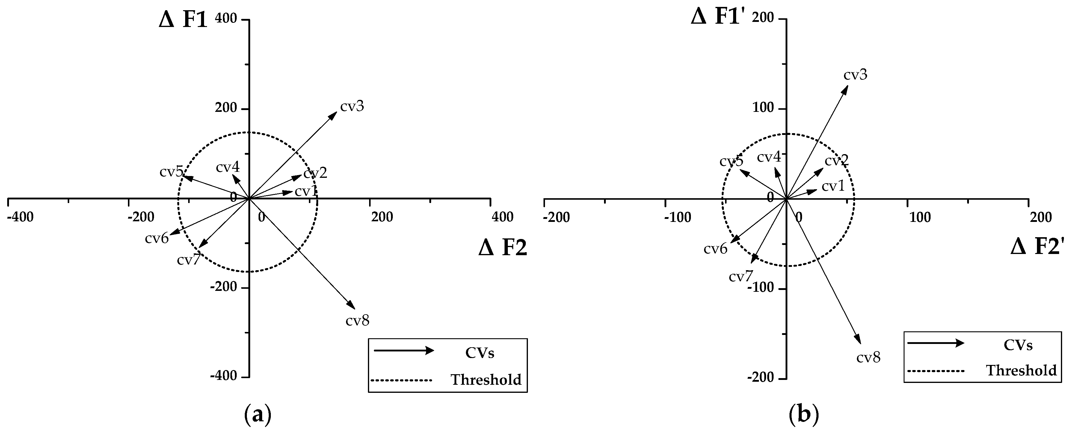
2.1. Magnitude and Direction of Change Vectors

The magnitudes of CVs in SAW-CVA carry the presence/absence of change information in n-D feature space. Similar to the standard CVA, the magnitude ρ of a CV in our proposed SAW-CVA is defined as:

$$\mathsf{\rho }=\sqrt{{\displaystyle \sum _{n=1}^N({\mathsf{\omega }}_n\cdot {(\mathsf{\Delta }{X}_n)}^2)}},\begin{array}{c}(0<{\mathsf{\omega }}_n<1,{\displaystyle \sum _{n=1}^N{\mathsf{\omega }}_n}=1)\end{array}$$

(3)

where ω_n is the weight of image feature n that controls the impact of different features on the magnitude of the CV, N is the number of features, and ΔX_n is the n-th component of the difference image ΔX. In the difference image ΔX, changed objects always have higher values than unchanged objects. Several approaches to extract the changed objects from the ΔX are based on automatic thresholding [25].

In 2-D CVA, the direction θ of a CV is calculated by:

$$\mathsf{\theta }=\arctan (\frac{\mathsf{\Delta }{X}_2}{\mathsf{\Delta }{X}_1}),\begin{array}{c}(-\frac{\mathsf{\pi }}{2}\le \mathsf{\theta }\le \frac{\mathsf{\pi }}{2})\end{array}$$

(4)

Because this procedure tends to be complex and impracticable for SAW-CVA, we elected to use the direction cosines procedure, which offers a more practical approach that can be extended to SAW-CVA. We use a direction variable α that effectively compresses the information on different types of change, to distinguish multiple changes in SAW-CVA. The direction variable α in our SAW-CVA is defined as:

$$\mathsf{\alpha }=\arccos \left({\displaystyle \sum _{n=1}^N({\mathsf{\omega }}_n\cdot \mathsf{\Delta }{X}_n)}/\sqrt{{\displaystyle \sum _{n=1}^N({\mathsf{\omega }}_n\cdot {(\mathsf{\Delta }{X}_n)}^2)}}\right),\begin{array}{c}(0\le \mathsf{\alpha }\le \mathsf{\pi },0<{\mathsf{\omega }}_n<1,{\displaystyle \sum _{n=1}^N{\mathsf{\omega }}_n}=1)\end{array}$$

(5)

where ω_n is the weight of image feature n that controls the impact of different features on the magnitude of the CV, N is the number of features, and ΔX_n is the n-th component of different image ΔX. All of direction variables in n-D feature space are defined in this way. These direction variables can be clustered into several classes representing different types of change.

2.2. Proposed Self-Adaptive Weight

Some researchers have used similar self-adaptive weighting in other fields of image analysis; they confirm that self-adaptive weights can retain the diversity of features for image analysis [26,27,28,29]. Wang et al. [26] propose a self-adaptive weight using prior knowledge, which is hard to extend to other studies. Similarly, Hu et al. [27] propose a self-adaptive weighting to estimate the contributions of texture, intensity and color features in image segmentation. An estimation probability was calculated according to a comparison with a given threshold, but this threshold setting also was not objective or convincing. In our study, we propose using the standard deviation (std) of an image object to calculate its self-adaptive weight.

The basic concept behind self-adaptive weights for our SAW-CVA approach is that the discrete degree of features in n-D feature space can be measured by the std of these image objects. The std of an image object denotes individual differences in the pixels of this object, and the dominant change feature of the image object can be identified by comparing the different std of all image objects. The richer the spectral feature of an image object, the lower its corresponding std compared with other features. Likewise, the richer the textural feature of an image object, the higher its corresponding std with respect to other features. Hence, if the std of image object is lower than a given threshold, then the dominant feature is a spectral feature; otherwise, the dominant feature is a textural feature [28]. Any given threshold is computed based on information from the whole image. The dominant feature reflects the main changed feature in the CVA.

Let ΔX_s and ΔX_t be the spectral and textural components of the difference image ΔX, then ΔX can be described by:

$$\mathsf{\Delta }X=\sqrt{{\mathsf{\omega }}_s{(\mathsf{\Delta }{X}_s)}^2+(1-{\mathsf{\omega }}_s){(\mathsf{\Delta }{X}_t)}^2}$$

(6)

where ω_s is the weight of the spectral feature, and (1 − ω_s) is the weight of the textural feature, respectively. Let the std of an image object at time t₁ and t₂ be std₁ and std₂, then their given thresholds are k₁ and k₂, respectively, and the weight of the spectral feature is described by:

$$\begin{array}{c}{\mathsf{\omega }}_s=\{\begin{array}{cc}\max (st{d}_1,st{d}_2)/(st{d}_1+st{d}_2),& ifst{d}_1<k_{1}andst{d}_2<k_2\\ \min (st{d}_1,st{d}_2)/(st{d}_1+st{d}_2),& other\end{array}\\ k_i=mea{n}_i+m_{i}st{d}_i,\text{i=1,2}\end{array}\}$$

(7)

where mean_i is the spectral mean value of the image object at time t_i, std_i is the spectral standard deviation of the image object at time t_i, and m_i is the self-adaptive index, such that −2 ≤ m_i ≤ 2.

To make full use of all change information of each spectral or textural feature, we use a weighted average of each feature as a component of ΔX_s and ΔX_t:

$$\begin{array}{c}{(\mathsf{\Delta }{X}_s)}^2={\displaystyle \sum _{i=1}^{N_s}{\mathsf{\omega }}_{si}{(\mathsf{\Delta }{X}_{si})}^2},{(\mathsf{\Delta }{X}_t)}^2={\displaystyle \sum _{i=1}^{N_t}{\mathsf{\omega }}_{ti}{(\mathsf{\Delta }{X}_{ti})}^2}\\ {\mathsf{\omega }}_{si}=\left|G_i\right|/{\displaystyle \sum _{i=1}^{N_s}\left|G_i\right|},{\mathsf{\omega }}_{ti}=\left|G_i\right|/{\displaystyle \sum _{i=1}^{N_t}\left|G_i\right|}\end{array}\}$$

(8)

where N_s and N_t are the number of spectral and textural features, ω_si and ω_ti are the corresponding weights of each spectral and textural feature, and G_i is the gradient of i-th feature.

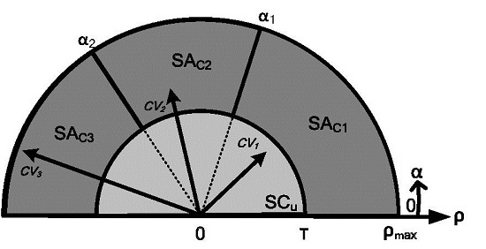
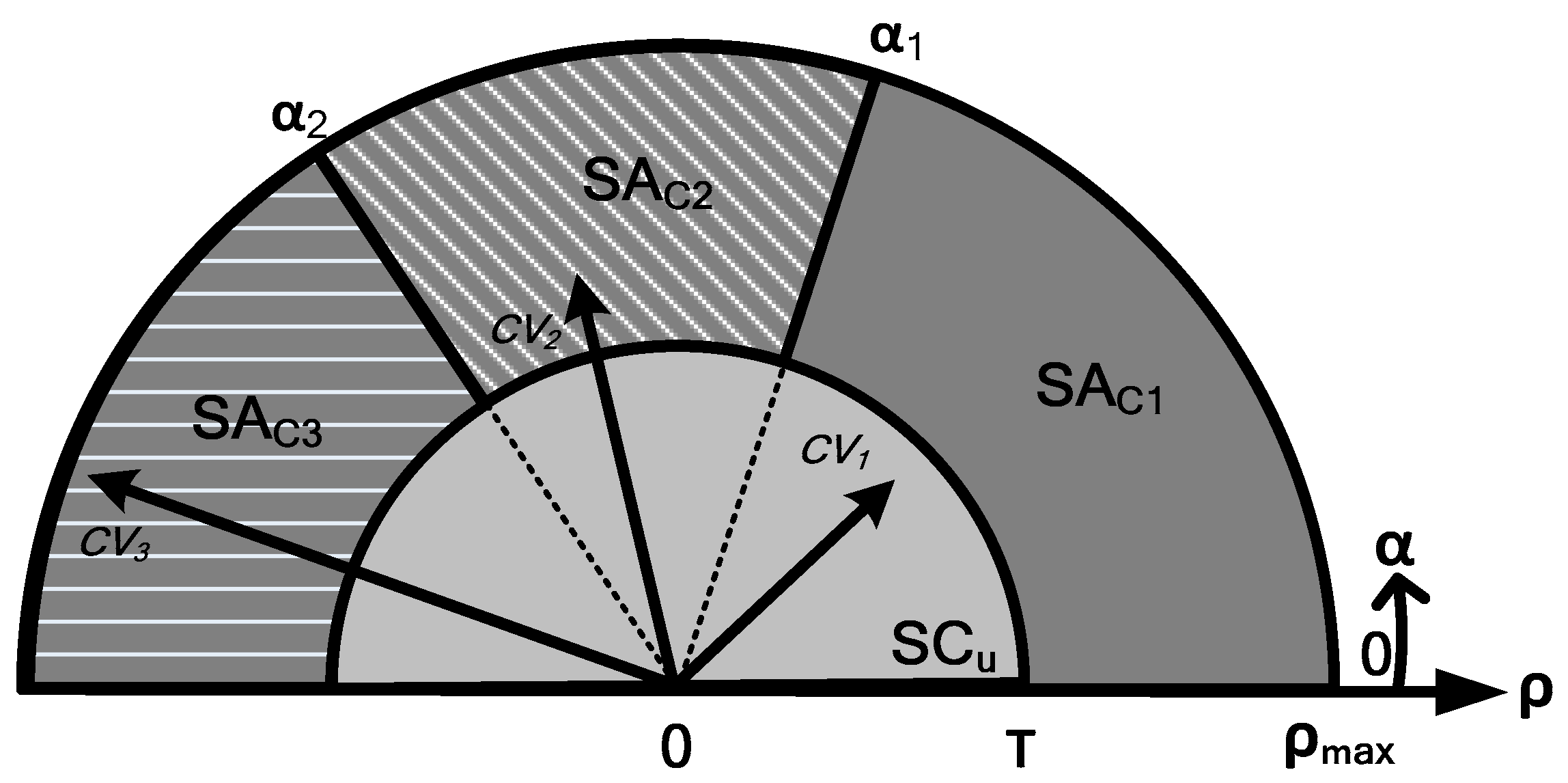
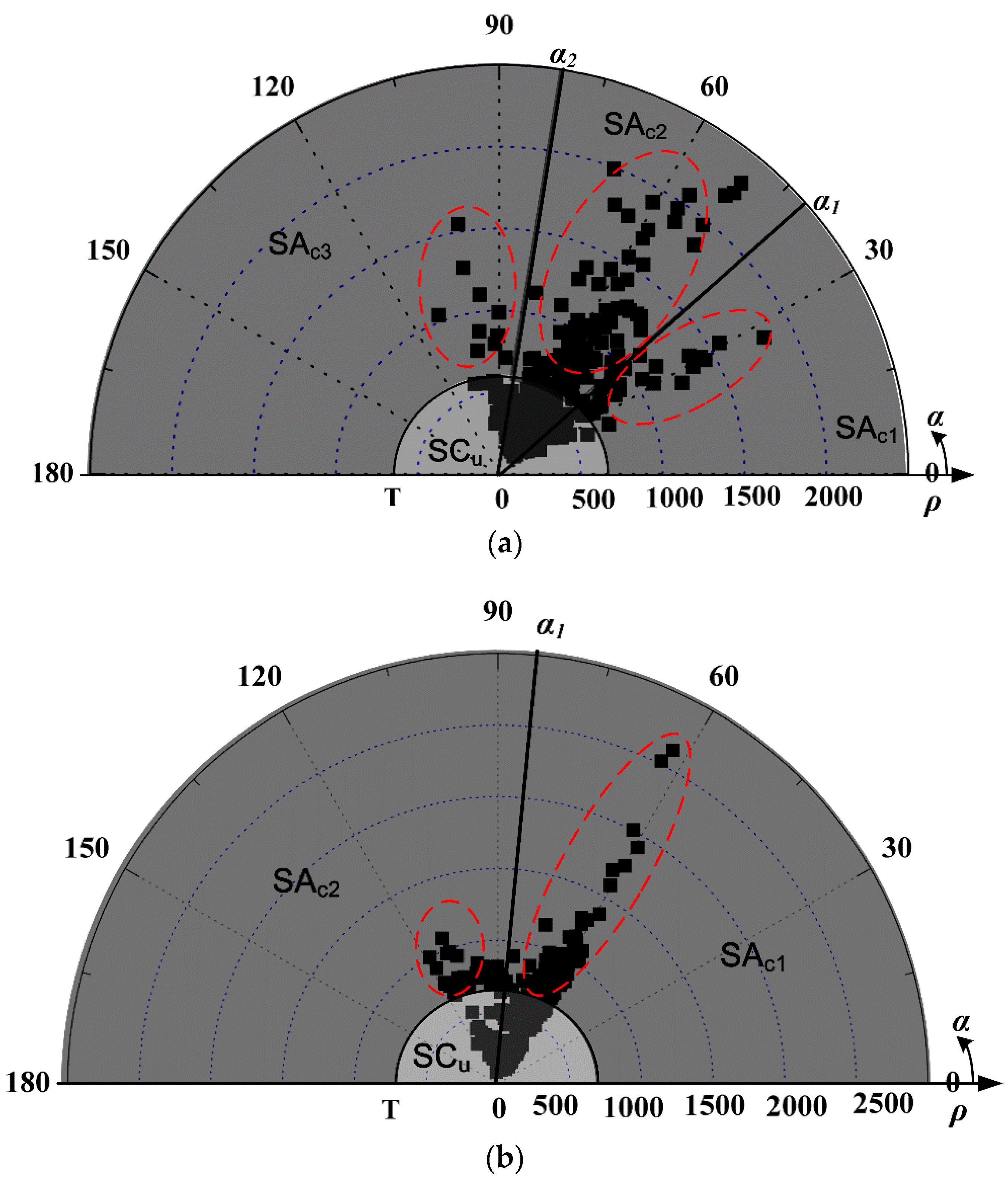
2.3. Representation of Proposed SAW-CVA

Standard CVA is described in a Cartesian coordinate system [6,8,19,20]. Here, we compare the standard CVA and the SAW-CVA in a Cartesian coordinate system using a 2-D feature space. In Figure 1a, eight CVs are represented in this system, three of them (CV3, CV6, CV8) exceed the range of the threshold circle, which indicates they represent changed image objects. After being given weights consistent with the standard CVA, our proposed SAW-CVA is represented in Figure 1b.

In Figure 1b, the coordinate axes have become ΔF1′ = ω₁ × ΔF1 and ΔF2′ = ω₂ × ΔF2. Now, four of the CVs exceed the range of the threshold circle (cv3, cv6, cv7 and cv8). In contrast to the standard CVA shown in Figure 1a, the image object corresponding to cv7 is now a changed object.

After defining all three components of the proposed SAW-CVA, these can be used to represent results in a polar coordinate system. The change detection problem can now be represented by multiple CVs. Although several studies of CVAs describe the magnitude and direction of 2-D CVA using a Cartesian coordinate system [6], it is complex and difficult to represent a SAW-CVA in this system. Thus, this paper uses the polar coordinate system described by Bovolo et al. [10] to represent the SAW-CVA. A polar representation of our proposed SAW-CVA with three CVs is shown in Figure 1.

Clearly, the proposed SAW-CVA domain is bounded by the ranges of both magnitude and direction variables (ρ and α). The domain consists of four parts, where the magnitude variable ρ determines the changed area, and direction variable determines the types of change. The first region is the semicircle SC_u of unchanged objects (light gray area; Figure 1), which is close to the origin of the domain. The other three regions form the semi-annulus SA_c of changed objects (dark gray area; Figure 1); they represent different types of change, as defined by direction variables α_k1 and α_k2. These regions are defined mathematically, as follows:

$$\begin{array}{l}S{C}_u=\left\{\mathsf{\rho },\mathsf{\alpha }:0\le \mathsf{\rho }\le T,0\le \mathsf{\alpha }\le \pi \right\}\\ S{A}_{c1}=\left\{\mathsf{\rho },\mathsf{\alpha }:T\le \mathsf{\rho }\le {\mathsf{\rho }}_{\max },0\le \mathsf{\alpha }\le {\mathsf{\alpha }}_1\right\}\\ S{A}_{c2}=\left\{\mathsf{\rho },\mathsf{\alpha }:T\le \mathsf{\rho }\le {\mathsf{\rho }}_{\max },{\mathsf{\alpha }}_1\le \mathsf{\alpha }\le {\mathsf{\alpha }}_2\right\}\\ S{A}_{c3}=\left\{\mathsf{\rho },\mathsf{\alpha }:T\le \mathsf{\rho }\le {\mathsf{\rho }}_{\max },{\mathsf{\alpha }}_2\le \mathsf{\alpha }\le \pi \right\}\end{array}\}$$

(9)

where T is the threshold value that discriminates changed and unchanged objects in the domain, while α₁ and α₂ are the two angular thresholds that separate different kinds of change. The location of each CV gives its compressed change information. For example, CV₁ located within SC_u represents an object that is not changed between t₁ and t₂, whereas CV₂ located in region of SA_c2 represents an object that has changed, having change type O_c2. Therefore, it is critical to define the thresholds T, α₁ and α₂ in our proposed SAW-CVA approach.

2.4. Proposed Technique for Multi-Feature Object-Based Change Detection

The proposed SAW-CVA for multi-feature OBCD has a two-step procedure: (1) extraction of the semi-annulus SA_c of all changed objects based on an analysis of histogram curvature of the magnitude variable ρ; and (2) identification of annular sectors in the semi-annulus SA_c based on analysis of the distribution of the direction variable α. The first step discriminates changed and unchanged objects, while the second step detects different types of change within the set of changed objects.

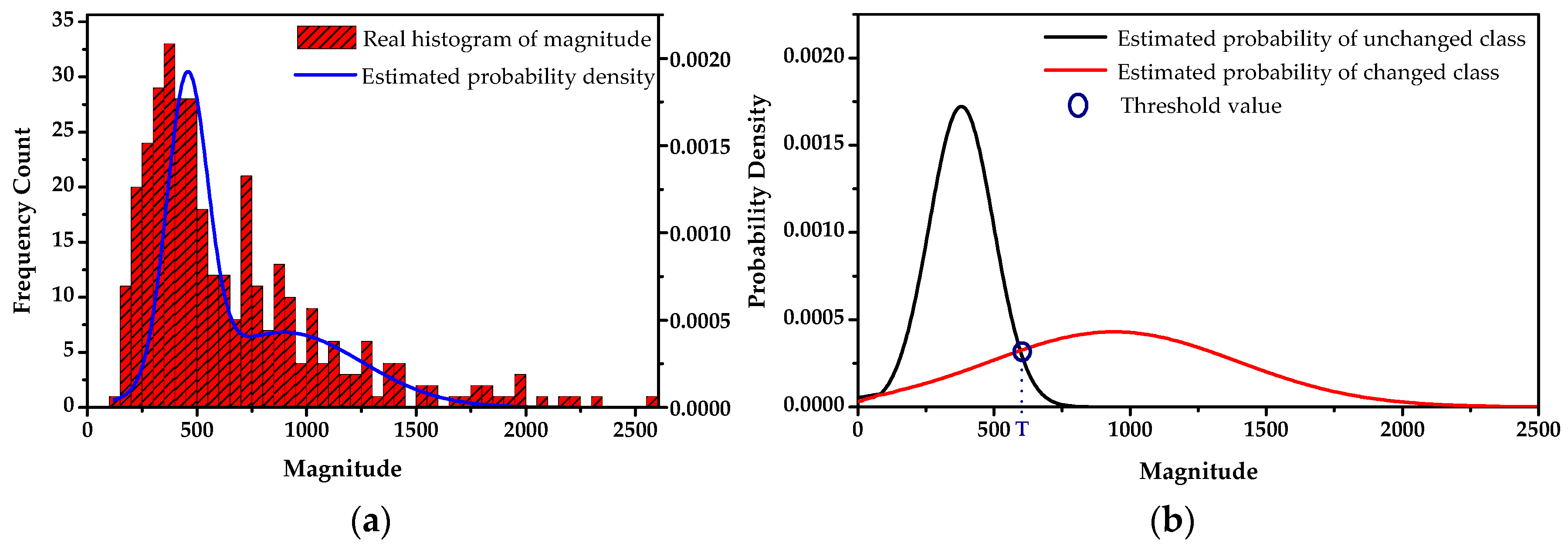
2.4.1. Extraction of Changed Objects

The changed objects are extracted by user-defined thresholds, which are utilized to distinguish the changed and unchanged objects. The prior knowledge is required to obtain the thresholds [30,31]. Because of the lack of observed data on the changed objects and the subjective interference of supervised threshold determination, we used the expectation-maximization (EM) algorithm [22,32] to define thresholds in an unsupervised way. This method has been widely used for change threshold determination [11,28,33]. Thus, changed objects are extracted based on threshold segmentation of the CVA magnitude image.

Let O = (O₁, O₂, …, O_I) be the set of image objects, and O_c, O_u be the class of changed objects and class of unchanged objects, respectively. Let P(O_c), P(O_u), p(ρ|O_c) and p(ρ|O_u) be the prior probabilities and the conditional probability density functions of classes O_c and O_u, respectively. Assuming that the distribution of the observed magnitude variable can be expressed as a mixture Gaussian distribution [34], then:

$$p({\mathsf{\rho }}_i)=P(O_c)p({\mathsf{\rho }}_i|O_c)+P(O_u)p({\mathsf{\rho }}_i|O_u)$$

(10)

where i is the number of image objects or CVs in the SAW-CVA, where i = (1, 2, …, I), and P(O_c) + P(O_u) = 1. According to the Bayes decision theory, the conditional probability of class l is given by:

$$p({\mathsf{\rho }}_i|l)=\exp (-{({\mathsf{\rho }}_i-{\mathsf{\mu }}_l)}^2/2{\mathsf{\delta }}_l^2)/\sqrt{2\mathsf{\pi }{\mathsf{\delta }}_l^2}$$

(11)

where the corresponding class probability p(l), the mean value μ_l, and the standard deviation δ_l are the parameters to be retrieved. As this defines a problem of parameter estimation with missing data, the EM algorithm can be used. The following iterative equations of the EM algorithm allow us to solve the estimation problem:

$$p^{t+1}(l)={\displaystyle \sum _{i=1}^I{p}^t(l|{\mathsf{\rho }}_i)}/I$$

(12)

$${\mathsf{\mu }}_l^{t+1}={\displaystyle \sum _{i=1}^I{p}^t(l|{\mathsf{\rho }}_i){\mathsf{\rho }}_i}/{\displaystyle \sum _{i=1}^I{p}^t(l|{\mathsf{\rho }}_i)}$$

(13)

$${\mathsf{\mu }}_l^{t+1}={\displaystyle \sum _{i=1}^I{p}^t(l|{\mathsf{\rho }}_i){\mathsf{\rho }}_i}/{\displaystyle \sum _{i=1}^I{p}^t(l|{\mathsf{\rho }}_i)}$$

(14)

where t is the iteration, and the initial values for all statistical parameters are computed using the K-means clustering algorithm. The procedure for obtaining our initial values using the EM algorithm is as follows: (1) using the K-means clustering algorithm to separate the classes O_c and O_u, obtain initial parameters for p(l), μ_l and δ_l; (2) update parameters p(l), μ_l and δ_l using Equations (12)–(14); and (3) repeat step 2 until the interval between two iterations is less than a given value [35]. Once the statistical parameters are estimated, the posterior probability of various classes is given by:

$$p(l|{\mathsf{\rho }}_i)=p({\mathsf{\rho }}_i|l)p(l)/p({\mathsf{\rho }}_i)$$

(15)

Bayes’s decision rule can be used for pattern labeling, whereby each image object O(i) is assigned to the class of changed or unchanged objects, using:

$$\{\begin{array}{cc}p(\mathsf{\rho }(i)|O_c)p(O_c)>p(\mathsf{\rho }(i)|O_u)p(O_u),& O_i\in O_c\\ p(\mathsf{\rho }(i)|O_c)p(O_c)\le p(\mathsf{\rho }(i)|O_u)p(O_u),& O_i\in O_u\end{array}$$

(16)

The threshold T used to separate the classes O_c and O_u can be obtained from the explicit solution of Equation (16).

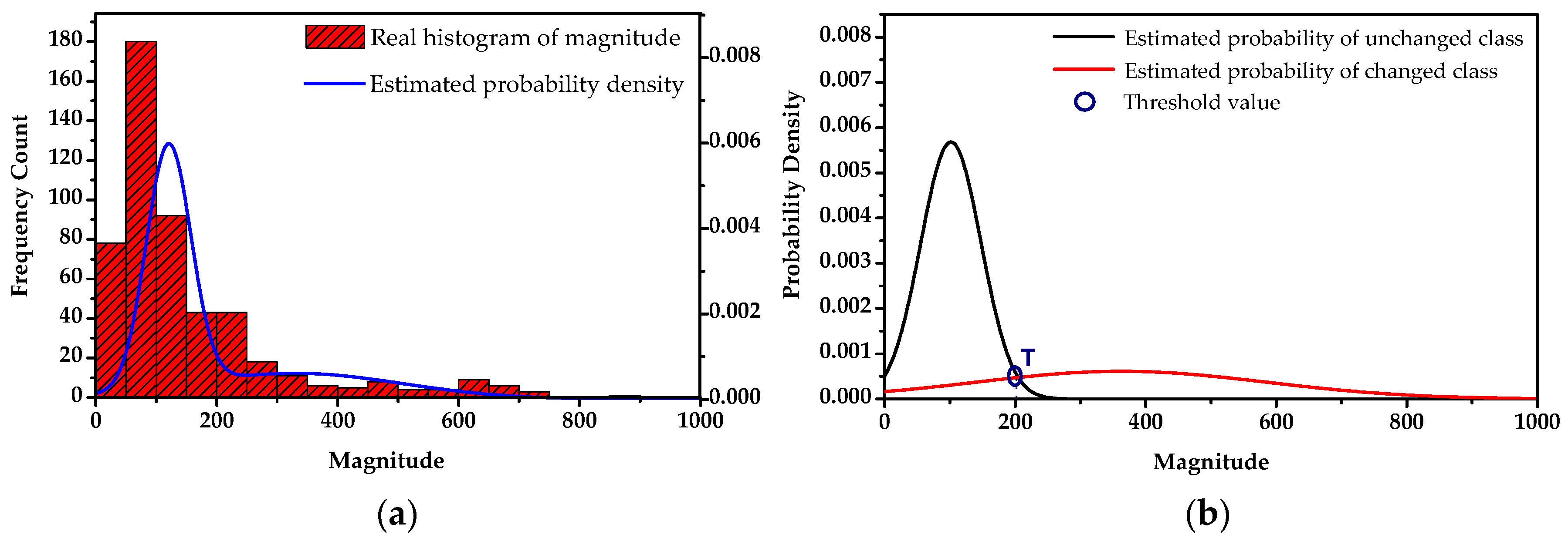
2.4.2. Identification of Different Types of Change

After the extraction of changed objects, attention is focused on separating the contributions of different possible types of change within the changed data set O_c = (O_c1, O_c2, …, O_ck). The different types of change O_ck are identified based on classification of the direction variable α. Because no prior knowledge about the location of the classes associated with different types of change can be acquired, the K-means clustering algorithm [32] is used to determine classes in an unsupervised way.

K-means clustering sorts data vectors into a predefined number of clusters, using Euclidean distance as the similarity measure. It is commonly used in computer vision as a form of data segmentation, where the purpose of data segmentation is to divide α into k clusters. If the direction variable set is α = (α₁, α₂, …, α_n), then the subset of data vectors that form cluster k is C_k. Its centroid is z_k, giving the clustering centroid set Z= (z₁, z₂, …, z_k). The objective function J also meets the clustering criterion:

$$J={\displaystyle \sum _{k=1}^K{\displaystyle \sum _{i=1}^n{\mathsf{\mu }}_k({\mathsf{\alpha }}_i)[d({\mathsf{\alpha }}_i,z_k)}}{]}^2$$

(17)

$$z_k=\frac{1}{N_k}{\displaystyle \sum _{\forall {\mathsf{\alpha }}_i\in {\mathrm{C}}_k}{\mathsf{\alpha }}_i}$$

(18)

where μ_k(α_i) is the membership degree of α_i to C_k; and $d({\mathsf{\alpha }}_i,z_k)=\Vert {\mathsf{\alpha }}_i-z_k\Vert$ is the Euclidean distance of z_k from α_i. The J is constructed using the minimum sum-of-squared-error criterion. For a cluster C_k, the mean vector z_k is the best vector to represent all samples in C_k in terms of minimizing the sum of the squared error vector d(α_i, z_k). Thus, J evaluates the sum of squared error generated from α, belonging to Z. Through iteration, the cluster centers continually move to make J as small as possible. During this process, the similarity of direction variables in the same cluster is gradually increased, while the similarity between different clusters is decreased. Iterations continue until the cluster centers no longer update. At this point, the pair of thresholds α_k1 and α_k2 in the direction domain for each kind of change have been defined. These thresholds are used to segment the different regions in a polar representation (SA_c1, SA_c2 and SA_c3; Figure 2). Now, each CV that falls in one of these regions is assigned to one of the identified kinds of change, according to Equation (9).

3. Experimental Results and Discussion

To validate the reliability and effectiveness of SAW-CVA to carry out multi-feature OBCD, two experiments were carried out on two pairs of remote sensing images. The first case is a change detection problem having 57 features in the Worldview-3 VHR multispectral images of farmland. The second case represents a change detection problem having 73 features in Worldview-2 VHR fusion images of a construction site. Details for each case are described below.

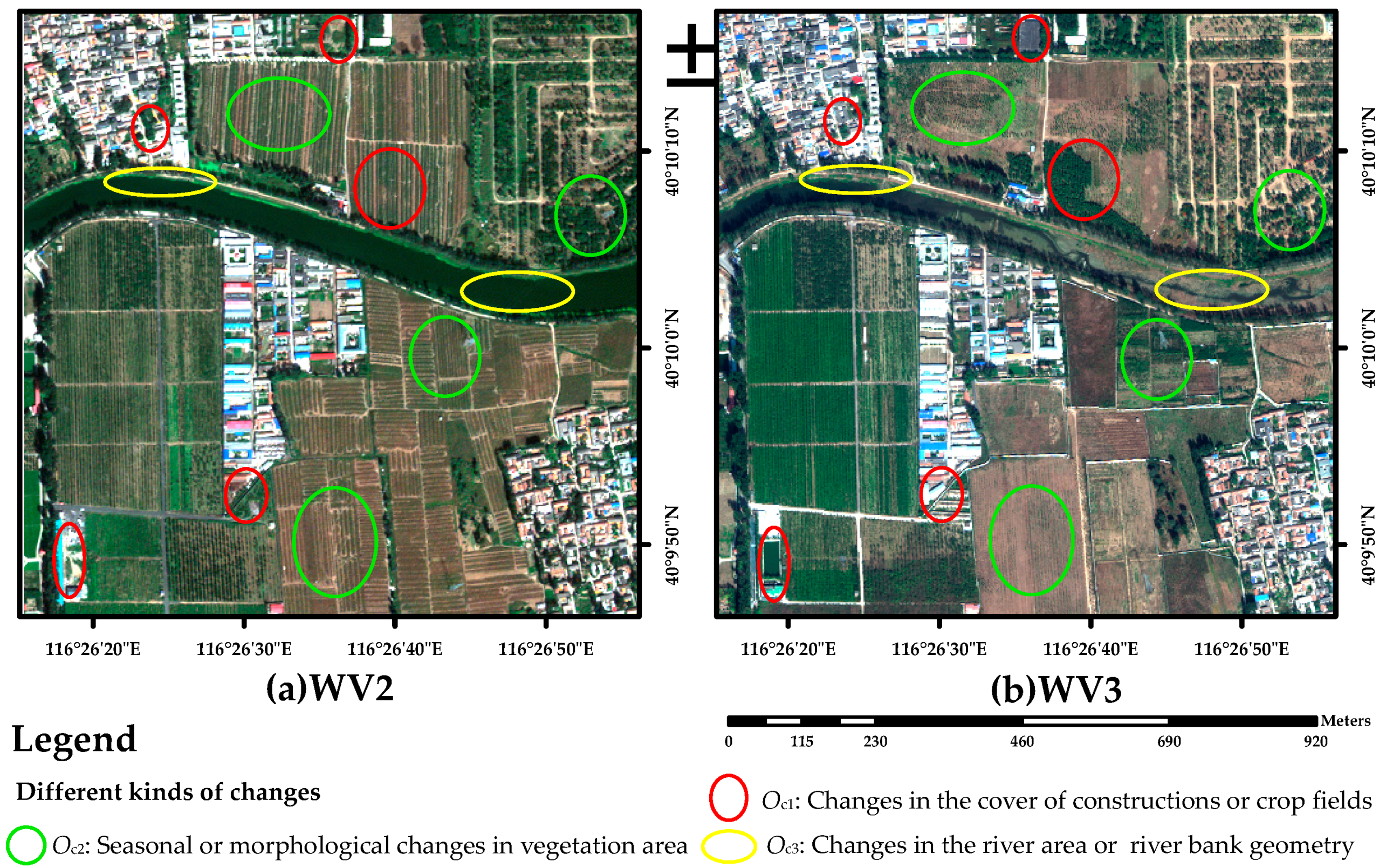
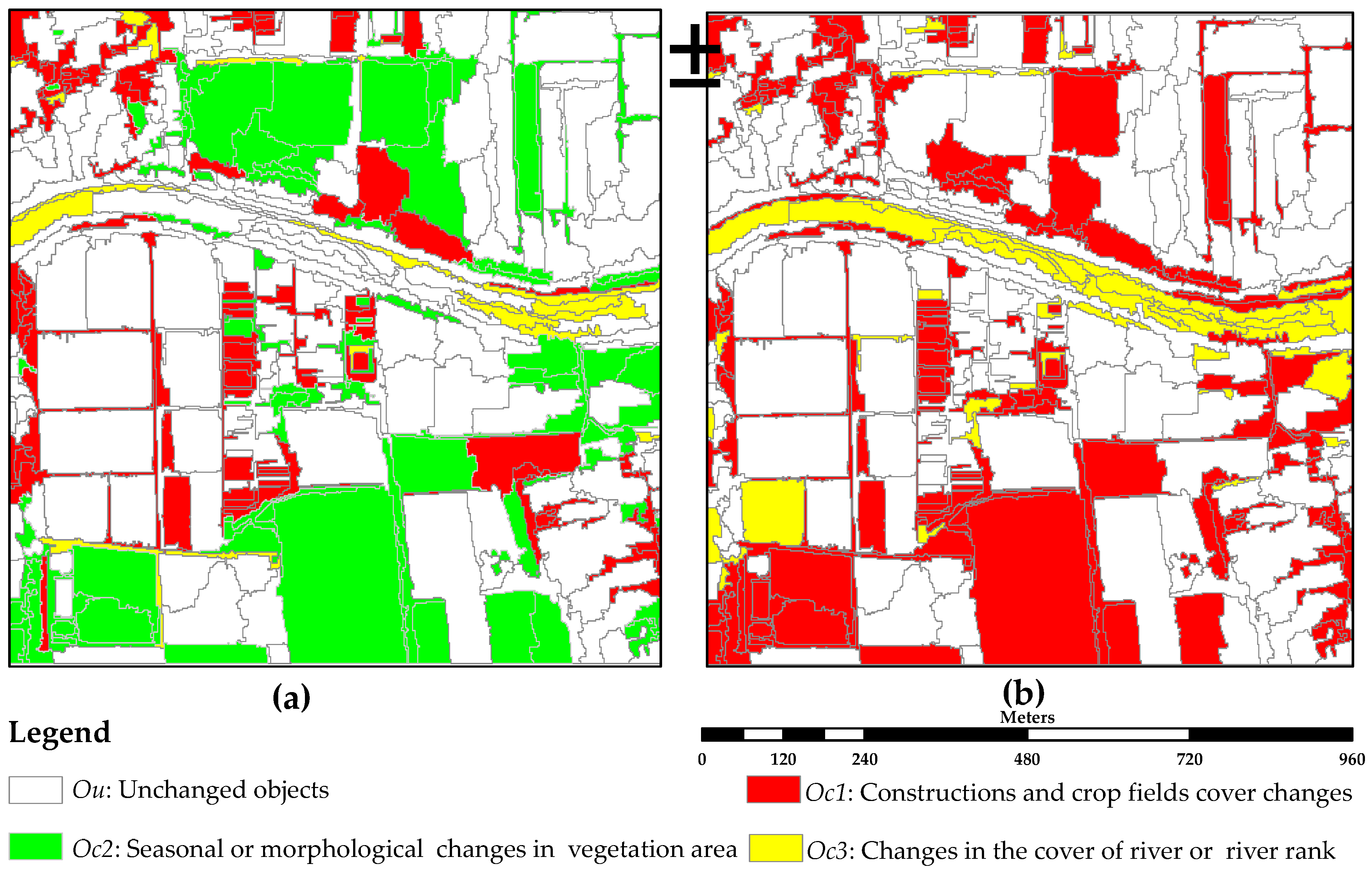
3.1. Case 1: Change Detection of Farmlands Using WV-3 VHR Multispectral Images

3.1.1. Material and Study Area

The first experimental case focuses on change detection in farmland; the data set is made up of a pair of Worldview-2/3 VHR images acquired on the Modern Agricultural Demonstrative Garden of Beijing (China) on 27 September 2010 and 20 October 2014. The spatial resolution of both remote sensing images is 1.8 m. Images have been cropped into sub-images of 500 × 500-pixel size with four spectral bands (blue, green, red and near-infra red). During data preprocessing, relative radiometric and geometric corrections were carried out to make the two images as comparable as possible. In the field of object-based image analysis, each image should be segmented into image objects, which are the basic unit of image analysis or processing. These two multiple-feature temporal images were segmented into 350 objects using the Multi-Resolution Segmentation (MRS) algorithm [36], available in eCognition Developer 9.2 software (Trimble Navigation Ltd., Sunnyvale, CO, USA). The parameters of MRS algorithm, such as scale, weight of shape criterion and weight of compactness criterion, were obtained by statistics-based automated parameters estimation [37]. In this study, we used the ESP (Estimation of Scale Parameter) tool [38] and calculated the mean value of local variance of image objects to obtain the optimal parameters by iterations on three levels. The optimal parameters (scale, weight of shape criterion and weight of compactness criterion) were set to be 130, 0.6 and 0.4, respectively. To guarantee that corresponding objects at different times were segmented exactly the same way, we carried out image segmentation on eight image layers overlain on the two images with the four spectral bands.

These images, corrected by true color synthesis, are shown in Figure 3. They show that there are three kinds of change that occurred between the two acquisition dates: (1) changes in construction or crop field areas, often related to new structures built to cover fields, labeled as O_c1; (2) seasonal or morphological changes to vegetated crop fields and wooded zones, labeled as O_c2; and (3) changes in the river area or the river bank geometry, related to a decrease in water level or river eutrophication, labeled as O_c3. The reference data set for the study area was defined after detailed field investigation, such that visual analysis involved some prior knowledge. This reference data set contained 203 changed image objects and 147 unchanged image objects. In detail, 104 objects were classed as O_c1, 73 objects as O_c2, and 26 objects as O_c3. Identification of these three kinds of change is very useful for evaluating crop growth or tillage condition of farmland, but distinguishing these three kinds of change, especially class O_c2, was critical to this case. Using the right feature selection of image objects, our SAW-CVA approach was able to extract changed objects and identify all three kinds of change.

3.1.2. Procedures and Results

First, the feature space of the image objects was built through the extraction and selection of features. Image object features mainly consist of spectral, geometric and textural characteristics. Although more kinds of features are helpful to OBCD, they can also lead to more interference or redundant information. It is necessary to extract and select the right features for OBCD. In this case, 57 features were ultimately extracted and selected to build a high dimensional feature space from the image objects. These features consisted of: mean value layers (four bands), their standard deviation layers (four bands), the normalized difference vegetation index, gray-level co-occurrence matrices (GLCM)-Contrast (4 bands × 4 directions), GLCM-Correlation (4 bands × 4 directions), and GLCM-Ang.2nd moment (4 bands × 4 directions) [39].

Second, we represented the change information in the SAW-CVA domain. According to the proposed framework for SAW-CVA described in Section 2, the self-adaptive weights of each feature were computed according to Equations (6)–(8), while the magnitude ρ and direction α of each CV were calculated using Equations (3) and (5), respectively. Figure 4a shows the polar scattergram for the SAW-CVA, in which changed objects define scatterpoints in the region SA_c (colored dark gray), and unchanged objects produce scatterpoints in the region SC_u (colored light gray). These two regions are separated by the threshold value T, obtained using the EM algorithm, as described in Section 2.4.1. Figure 5a shows the real distribution of the histogram for the magnitude of CVs (red bars), and the distribution of estimated parameters from a mixture of Gaussian distributions (black line). It can be seen that the estimated distribution is well-fitted to the real distribution, which confirms that a reasonable approximation was obtained with the EM algorithm. The threshold value T used to distinguish the changed and unchanged class can be identified through comparison between P(O_c)p(ρ_i|Oc) (red line) and P(O_u)p(ρ_i|O_u) (black line) in Figure 5b, giving a threshold T = 600.

Third, to separate contributions from different kinds of change, threshold values also were identified using K-means clustering, as described in Section 2.4.2. In Figure 4a, which shows the scattergram obtained from SAW-CVA in polar representation, three clusters can be identified with high magnitude and three distinct directions. These three clusters corresponding to three kinds of change are divided by the two angular thresholds α₁ and α₂, according to Equations (17) and (18), where K = 3 in Equation (17) gives angular thresholds α₁ = 42°, α₂ = 80°. After carrying out the thresholding procedure, the regions shown in Figure 4a can be defined mathematically, as follows:

$$\begin{array}{l}S{C}_u=\left\{\mathsf{\rho },\mathsf{\alpha }:0\le \mathsf{\rho }\le 600,0^{°}\le \mathsf{\alpha }\le {180}^{°}\right\}\\ S{A}_{c1}=\left\{\mathsf{\rho },\mathsf{\alpha }:600\le \mathsf{\rho }\le 2500,0^{°}\le \mathsf{\alpha }\le {42}^{°}\right\}\\ S{A}_{c2}=\left\{\mathsf{\rho },\mathsf{\alpha }:600\le \mathsf{\rho }\le 2500,{42}^{°}\le \mathsf{\alpha }\le {80}^{°}\right\}\\ S{A}_{c3}=\left\{\mathsf{\rho },\mathsf{\alpha }:600\le \mathsf{\rho }\le 2500,{80}^{°}\le \mathsf{\alpha }\le {180}^{°}\right\}\end{array}\}$$

(19)

where sectors SC_u, SA_c1, SA_c2 and SA_c3 are associated with classes O_u, O_c1, O_c2 and O_c3, respectively.

To compare with our SAW-CVA approach, the scattergram in the polar domain for a standard CVA is shown in Figure 4b. The standard CVA has no self-adaptive weighting for each feature, which means that the weight of each feature has ω = 1. Under a Gaussian assumption, the EM algorithm estimates the threshold T = 680, using Equations (10)–(16). Because only two sectors can be identified in Figure 4b, the value of K was set to 2, and the threshold α₁ = 84° was computed using K-means clustering criteria, as outlined in Equations (17) and (18).

Using these threshold values (both for magnitude and direction) to classify the image objects obtained from multi-resolution segmentation, the OBCD result maps were computed based on SAW-CVA and standard CVA in Figure 6. As expected, three kinds of change have been identified and coded using different colors in the SAW-CVA (Figure 6a), but only two kinds of change are identified in the OBCD map produced using a standard CVA (Figure 6b).

3.1.3. Analysis and Discussion

A quantitative analysis of the results achieved using these two approaches is shown in

Table 1. The accuracy assessment for the OBCD result obtained by the proposed SAW-CVA approach.

SAW-CVA		True Class				FPR or User Accuracy
		Ou	Oc1	Oc2	Oc3
Resulting Class	Ou	136	3	3	2	94.44%
	Oc1	3	78	2	2	91.76%
	Oc2	8	21	67	2	68.37%
	Oc3	0	2	1	20	86.96%
FNR or Producer Accuracy		92.52%	75.00%	91.78%	76.92%
Overall Accuracy		86.03%		Kappa	0.7976

and

Table 2. The accuracy assessment for the OBCD result obtained by the standard CVA approach.

Standard CVA		True Class				FPR or User Accuracy
		Ou	Oc1	Oc2	Oc3
Resulting Class	Ou	130	2	25	0	82.80%
	Oc1	10	100	38	1	67.11%
	Oc2	0	0	0	0	0.00%
	Oc3	7	2	10	25	56.82%
FNR or Producer Accuracy		88.44%	96.15%	0.00%	96.15%
Overall Accuracy		75.86%		Kappa	0.6283

. Using the reference data set, data in these tables were computed with an error confusion matrix. An error confusion matrix is constructed to validate the accuracy of OBCD in the whole image area. The accuracy evaluation for the OBCD results is based on a false positive rate (FPR), a false negative rate (FNR), overall accuracy (OA), and Kappa accuracy. The FPR and FNR denote the possibility of false detection and missing detection, respectively.

From Table 1 and Table 2, it is clear that SAW-CVA has much better precision in its OBCD result, relative to the standard CVA. The OA and Kappa accuracy of SAW-CVA (86.03%, 0.7976) also are higher than the standard CVA (75.86%, 0.6283). The standard CVA allows us to detect only two kinds of change, while SAW-CVA detected three kinds. Some seasonal or structural changes in vegetated area were not easily and fully identified by standard CVA, with the objects belonging to O_c2 being wrongly divided into other classes in Table 2. It is worth noting that despite many false detections for O_c2 and missing detections for O_c1 in our SAW-CVA approach, Table 1 shows that the FPR of O_c2 (68.37%) and FNR of O_c1 (75%) are lower than other values. Therefore, our proposed SAW-CVA approach effectively detected most information about change available in the representative sample, based on our accuracy assessment of the OBCD results.

This experiment confirms that the proposed SAW-CVA approach can identify different kinds of change and is more effective than a standard CVA. However, noise still exists, leading to some false detections of O_c2, especially when differentiating O_c2 from O_c1. Clearly, we also need to evaluate the effect of feature selection on the SAW-CVA approach for multi-feature OBCD.

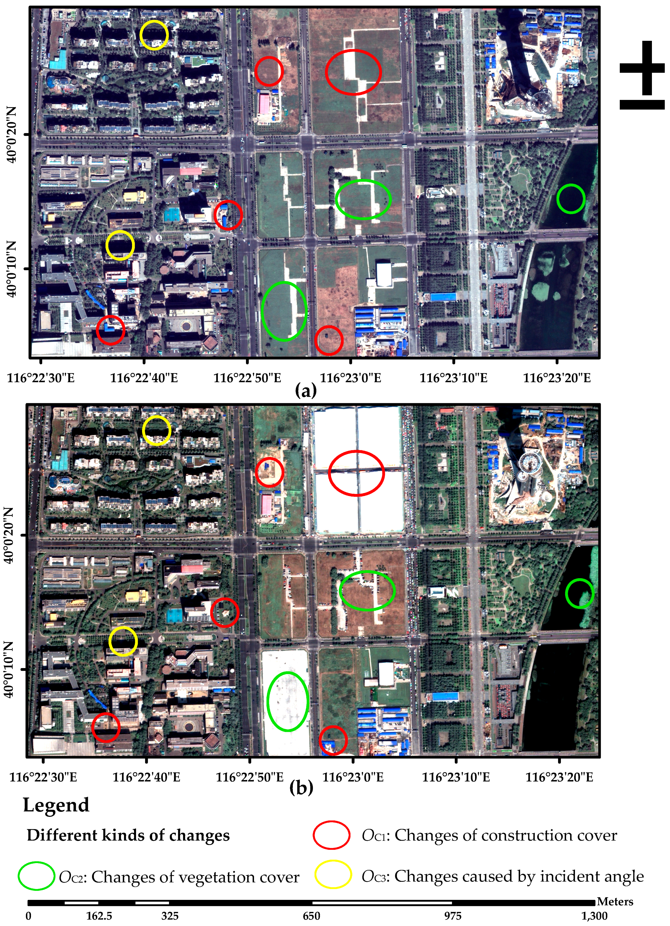
3.2. Case 2: Change Detection for Construction Sites Using WV-2 VHR Panchromatic Fusion Images

3.2.1. Material and Study Area

This experiment was conducted on Worldview-2 VHR images, acquired on the area around Beijing Olympic Park (China) on 12 September 2012 and 20 September 2013, respectively. Image preprocessing included pan-sharpening, registration and relative radiometric corrections. Gram-Schmidt Pan Sharpening [40] has been used on fusion images integrated from a panchromatic channel and four bands of multispectral images. As for Case 1, the registration process uses a nearest neighbor interpolation, with 15 ground control points. The relative radiometric correction applies robust regression to normalize images, subtracting from each spectral channel with reference to 202 pseudo invariant features.

The final data set was cropped into images of 2500 × 1500-pixel size, with a spatial resolution of 0.5 m. These experimental images were segmented into 512 objects. In this study, the optimal parameters (scale, weight of shape criterion and weight of compactness criterion) were set to be 120, 0.7 and 0.3, respectively. Three kinds of change can be observed (Figure 7): O_c1 denotes changed objects on buildings or other construction areas, O_c2 denotes changed objects in grassland or other vegetated areas, and O_c3 denotes changed objects caused by the shooting angle offset of the sensor. It is worth noting that O_c3 does not represent a real class of changed objects, but comprises artifacts related to differences in shooting angle of the sensor, which causes changes to the shadows of high buildings.

The study area, located in the urban center, has complicated change information, which is hard to identify using a standard CVA approach. In particular, pseudo or slightly changed objects are hard to identify. Hence, the purpose of this case was to verify whether the proposed SAW-CVA approach could detect slight change or pseudo change.

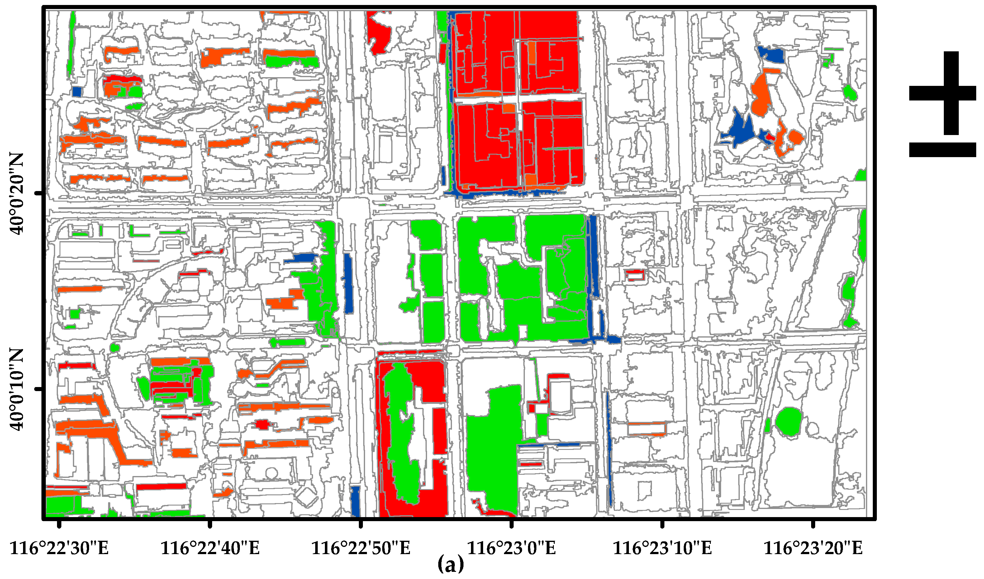
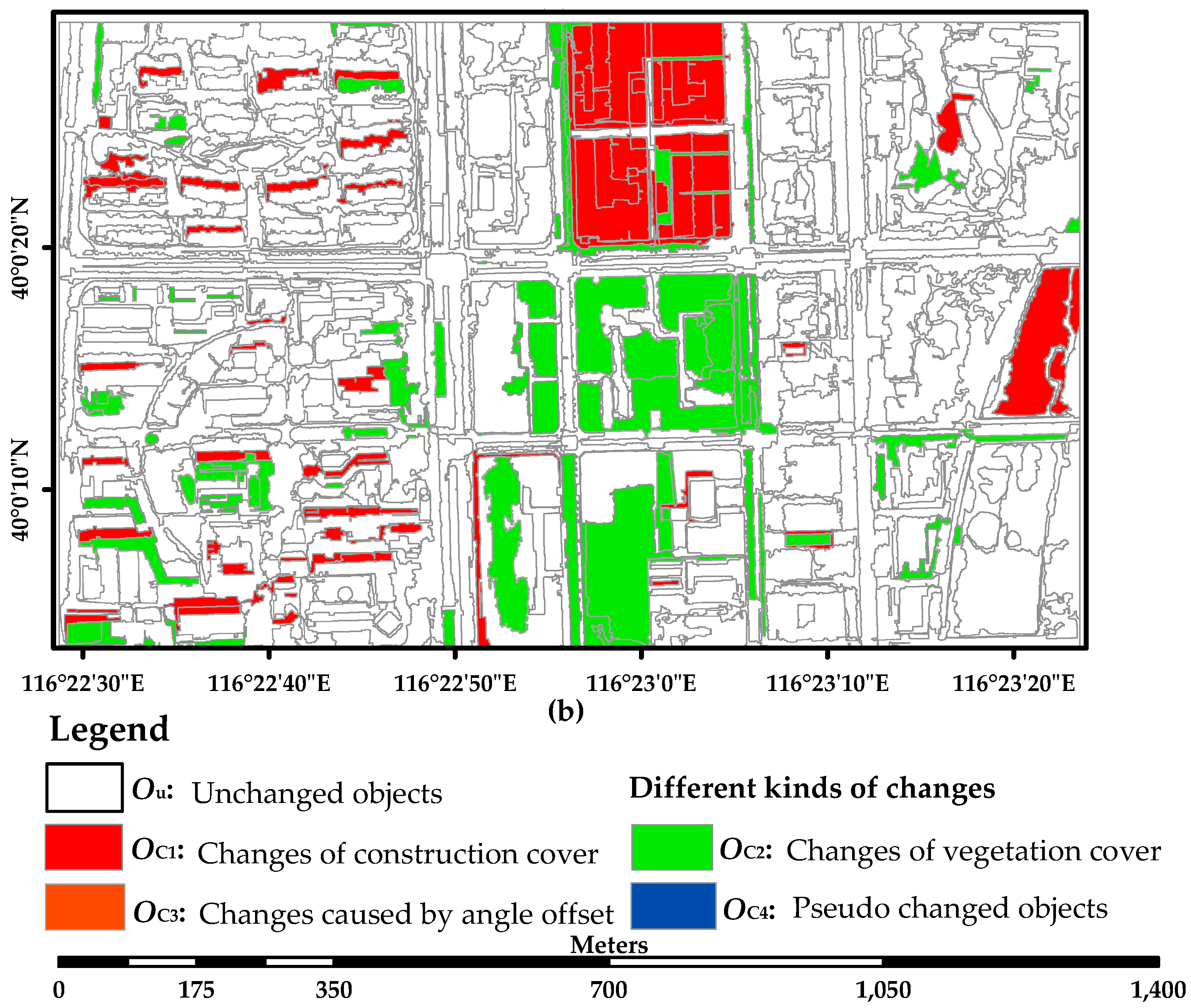
3.2.2. Procedures and Results

For this fusion data set, 73 features were selected to compute the magnitude and angle of each CV in the image objects. Image object features consisted of mean value layers (4 bands), standard deviation layers (4 bands), the normalized difference vegetation index, GLCM-Contrast (4 bands × 4 directions), GLCM-Entropy (4 bands × 4 directions), GLCM-Ang.2nd moment (4 bands × 4 directions), and GLCM-Mean (4 bands × 4 directions). Figure 8a shows the scatter of results of the SAW-CVA, with a threshold value T = 235 that separates O_u and O_c obtained using the EM algorithm (Figure 9). Clearly, the reliability of the EM algorithm is confirmed in Figure 9a because our visual analysis shows that the estimated distribution (blue line) fits the behavior of the real histogram (red bars).

Four main clusters were identified in the polar representation of our SAW-CVA (Figure 8a). These four sectors were defined using angular thresholds α₁, α₂ and α₃. According to the K-means clustering algorithm described in Section 2.4.2, SA_c1 is made up of CVs with α∈[(0°, 32°), SA_c2 with α∈[32°, 65°), SA_c3 with α∈[65°, 113°), and SA_c4 with α∈[113°, 180°). According to the reference data, it can be shown that objects associated with O_c1 fall within SA_c2, objects associated with O_c2 fall within SA_c4, objects associated with O_c3 fall within SA_c1. Otherwise, objects in SA_c3 are associated with pseudo changes created by shadows of high buildings, or cars on the road, and are labeled as O_c4. To compare with our SAW-CVA approach, a scattergram in the polar domain for the standard CVA is shown in Figure 8b. Under a Gaussian assumption, the EM algorithm estimates its threshold T = 180, yielding only two sectors in Figure 8b. Setting the value of K to 2, a threshold having α₁ = 88° was computed using the K-means clustering algorithm.

Using the threshold values estimated with our proposed SAW-CVA approach, OBCD maps were generated (Figure 10). Four kinds of change can be identified in Figure 10a, although classes O_c3 and O_c4 belong to the unchanged class in the real situation. The reference data set, defined from visual analysis of the Google Earth image and detailed field investigations, contains 347 unchanged objects and 165 changed objects. Of these, 53 objects are related to O_c1, and 112 objects are related to O_c2. Compared with the OBCD map for the standard CVA, our SAW-CVA approach was able to distinguish most of the pseudo changed objects from real changed objects, although differences exist in the kinds of change identified in the OBCD result and the ground truth data.

3.2.3. Analysis and Discussion

A quantitative analysis of the results obtained using these two approaches is shown in

Table 3. The accuracy assessment for the OBCD result obtained by the proposed SAW-CVA approach.

SAW-CVA		True Class					FPR or User Accuracy
		Ou	Oc1	Oc2	Oc3	Oc4
Resulting Class	Ou	346	4	3	2	0	97.46%
	Oc1	2	38	6	3	0	77.55%
	Oc2	6	5	36	5	0	69.23%
	Oc3	8	2	2	32	0	72.73%
	Oc4	10	1	0	1	0	0.00%
FNR or Producer Accuracy		93.01%	76.00%	76.60%	74.42%	0.00%
Overall Accuracy		88.28%		Kappa	0.7508

and

Table 4. The accuracy assessment for the OBCD result obtained by the standard CVA approach.

CVA		True Class				FPR or User Accuracy
		Ou	Oc1	Oc2	Oc3
Resulting Class	Ou	356	6	4	9	94.93%
	Oc1	3	38	2	24	56.72%
	Oc2	13	6	41	10	58.57%
	Oc3	0	0	0	0	0.00%
FNR or Producer Accuracy		95.70%	76.00%	87.23%	0.00%
Overall Accuracy		84.96%		Kappa	0.6601

. These data were computed using the error confusion matrix. Clearly, the SAW-CVA has higher accuracy (88.28%, 0.7508) than the standard CVA (84.96%, 0.6601). The standard CVA approach could not distinguish between artifacts caused by the incident angle of the sensor from changes to roof cover. It is worth noting that some noise and pseudo changed objects are still visible in both OBCD maps, slightly affecting the accuracy of other classes (Table 3). Overall, we conclude that the proposed SAW-CVA approach and the estimations obtained using the EM algorithm are effective and reliable, according to quantitative analysis of the OBCD results. Moreover, although the proposed SAW-CVA approach makes some false detections for pseudo changed objects, it was able to separate this kind of change from other change classes.

Clearly, the experimental results have shown that our proposed SAW-CVA approach is able to identify some pseudo or slightly changed objects in the context of a complex urban environment. The results also reveal that our technique was not able to reduce or eliminate the interference of shadows in OBCD in an urban context.

4. Conclusions

Here, we propose an automatic technique for object-based change detection (OBCD) of multiple features in very high resolution (VHR) remote sensing images, referred to as Self-Adaptive Weight-Change Vector Analysis (SAW-CVA). Our SAW-CVA approach uses CVA with self-adaptive weights to solve n-D OBCD problems (where n is the number of features or channels acquired by the image objects or sensor). It computes the magnitude of change vectors (CVs) and direction (angle) between the difference vector and a reference one. Unlike the standard CVA in a Cartesian coordinate system, the proposed SAW-CVA approach is presented in a polar coordinate system, which better preserves the change information present in all CVs. The CVs also have been stretched to be more easily distinguished. This representation assists visualization of change information, without the need to select a pair of spectral channels, as for a standard CVA. Our proposed approach uses the expectation-maximization (EM) algorithm to estimate the threshold to extract changed objects under a Gaussian assumption. It also uses the K-means clustering algorithm to classify or identify different kinds of changes. These thresholds define sectors in the polar domain of our SAW-CVA, which represent different changed object classes.

Two experiments carried out on Worldview-3 VHR multispectral images and Worldview-2 panchromatic fusion images confirmed the effectiveness of our SAW-CVA approach for change detection in farmlands and construction sites. Both qualitative and quantitative results indicate that the SAW-CVA approach has better capabilities in OBCD than the standard CVA; this also confirms the suitability of the EM algorithm used in our approach. Our SAW-CVA was able to retrieve the main information related to change and to distinguish all the different kinds of change present at our field sites. In particular, the proposed SAW-CVA can identify seasonal and structural changes in vegetated areas (as shown in Case 1), and separate pseudo changes and artifacts caused by the shooting angle of the sensor from real changes (as shown in Case 2). This suggests that the SAW-CVA can preserve more change information than a standard CVA, in which the dimension reduction process results in loss of information about the distribution of different kinds of change. However, there were some false or missing detections caused by noise in the OBCD results using SAW-CVA.

In contrast to the standard CVA, the advantages of our SAW-CVA are three-fold. First, the SAW-CVA approach is able to identify multiple kinds of change because it can retain the difference of directions of CVs simultaneously. Second, the SAW-CVA approach is more accurate than the standard CVA, because it can preserve more change information using self-adaptive weights to control the contribution of each type of feature. Third, when using polar representation to show the distribution of CVs, the CVs obtained using the SAW-CVA approach have more diversity than the standard CVA, which is useful to extract changed samples and distinguish different samples.

In future work, it would be worthwhile to exploit the potential of the SAW-CVA technique for noise elimination, when using SAW-CVA in the context of more complex OBCD problems. It also needs further experimental validation because edge effects may affect the std of the image object. Finally, we plan to analyze the sensitivity of SAW-CVA to exploit multiscale or multiresolution information intrinsically present in VHR images.

References

1. Blaschke, T.; Hay, G.J.; Kelly, M.; Lang, S.; Hofmann, P.; Addink, E.; Queiroz Feitosa, R.; van der Meer, F.; van der Werff, H.; van Coillie, F.; et al. Geographic object-based image analysis—Towards a new paradigm. ISPRS J. Photogramm. 2014, 87, 180–191. [Google Scholar] [CrossRef] [PubMed]
2. Blaschke, T. Object based image analysis for remote sensing. ISPRS J. Photogramm. 2010, 65, 2–16. [Google Scholar] [CrossRef]
3. Malila, W.A. Change vector analysis: An approach for detecting forest changes with landsat. In Proceedings of 6th Annual Symposium on Machine Processing of Remotely Sensed Data Soil Information Systems and Remote Sensing and Soil Survey, West Lafayette, IN, USA, 3–6 June 1980.
4. Tewkesbury, A.P.; Comber, A.J.; Tate, N.J.; Lamb, A.; Fisher, P.F. A critical synthesis of remotely sensed optical image change detection techniques. Remote Sens. Environ. 2015, 160, 1–14. [Google Scholar] [CrossRef]
5. Zhuang, H.; Deng, K.; Fan, H.; Yu, M. Strategies combining spectral angle mapper and change vector analysis to unsupervised change detection in multispectral images. IEEE Geosci. Remote Sens. 2016, 13, 681–685. [Google Scholar] [CrossRef]
6. Nackaerts, K.; Vaesen, K.; Muys, B.; Coppin, P. Comparative performance of a modified change vector analysis in forest change detection. Int. J. Remote Sens. 2005, 26, 839–852. [Google Scholar] [CrossRef]
7. Chen, J.; Gong, P.; He, C.; Pu, R.; Shi, P. Land-use/land-cover change detection using improved change-vector analysis. Photogramm. Eng. Rem. Sens. 2003, 69, 369–379. [Google Scholar] [CrossRef]
8. Johnson, R.D.; Kasischke, E.S. Change vector analysis: A technique for the multispectral monitoring of land cover and condition. Int. J. Remote Sens. 1998, 19, 411–426. [Google Scholar] [CrossRef]
9. Maeda, E.E.; Arcoverde, G.F.B.; Pellikka, P.K.E.; Shimabukuro, Y.E. Fire risk assessment in the brazilian amazon using modis imagery and change vector analysis. Appl. Geogr. 2011, 31, 76–84. [Google Scholar] [CrossRef]
10. Bovolo, F.; Bruzzone, L. A theoretical framework for unsupervised change detection based on change vector analysis in the polar domain. IEEE Trans. Geosci. Remote 2007, 45, 218–236. [Google Scholar] [CrossRef]
11. Bovolo, F.; Marchesi, S.; Bruzzone, L. A framework for automatic and unsupervised detection of multiple changes in multitemporal images. IEEE Trans. Geosci. Remote 2012, 50, 2196–2212. [Google Scholar] [CrossRef]
12. Xiaolu, S.; Bo, C. Change detection using change vector analysis from landsat TM images in Wuhan. Procedia Environ. Sci. 2011, 11, 238–244. [Google Scholar] [CrossRef]
13. Chen, Y.H.; Xiao bing, L.I.; Chen, J.; Shi, P.J. The change of NDVI time series based on change vector analysis in china, 1983–1992. J. Remote Sens. 2002, 6, 12–18. [Google Scholar]
14. Allen, T.R.; Kupfer, J.A. Application of spherical statistics to change vector analysis of Landsat data : Southern appalachian spruce–fir forests. Remote Sens. Environ. 2000, 74, 482–493. [Google Scholar] [CrossRef]
15. Warner, T. Hyperspherical direction cosine change vector analysis. Int. J. Remote Sens. 2005, 26, 1201–1215. [Google Scholar] [CrossRef]
16. Bovolo, F.; Bruzzone, L.; Marconcini, M. A novel approach to unsupervised change detection based on a semisupervised SVM and a similarity measure. IEEE T. Geosci. Remote 2008, 46, 2070–2082. [Google Scholar] [CrossRef]
17. He, C.; Wei, A.; Shi, P.; Zhang, Q.; Zhao, Y. Detecting land-use/land-cover change in rural–urban fringe areas using extended change-vector analysis. Int. J. Appl. Earth Obs. Geoinformation 2011, 13, 572–585. [Google Scholar] [CrossRef]
18. Thonfeld, F.; Feilhauer, H.; Braun, M.; Menz, G. Robust change vector analysis (RCVA) for multi-sensor very high resolution optical satellite data. Int. J. Appl. Earth Obs. Geoinform. 2016, 50, 131–140. [Google Scholar] [CrossRef]
19. Xian, G.; Homer, C. Updating the 2001 national land cover database impervious surface products to 2006 using landsat imagery change detection methods. Remote Sens. Environ. 2010, 114, 1676–1686. [Google Scholar] [CrossRef]
20. Carvalho Júnior, O.A.; Guimarães, R.F.; Gillespie, A.R.; Silva, N.C.; Gomes, R.A.T. A new approach to change vector analysis using distance and similarity measures. Remote Sens. 2011, 3, 2473–2493. [Google Scholar] [CrossRef]
21. Singh, A. Review article digital change detection techniques using remotely-sensed data. Int. J. Remote Sens. 1989, 10, 989–1003. [Google Scholar] [CrossRef]
22. Bruzzone, L.; Prieto, D.F. Automatic analysis of the difference image for unsupervised change detection. IEEE Trans. Geosci. Remote 2000, 38, 1171–1182. [Google Scholar] [CrossRef]
23. Prieto, L.B.; Fernandez, D. A minimum-cost thresholding technique for unsupervised change detection. Int. J. Remote Sens. 2000, 21, 3539–3544. [Google Scholar]
24. Celik, T.; Ma, K.K. Unsupervised change detection for satellite images using dual-tree complex wavelet transform. IEEE Trans. Geosci. Remote 2010, 48, 1199–1210. [Google Scholar] [CrossRef]
25. Radke, R.J.; Srinivas, A.; Omar, A.K.; Badrinath, R. Image change detection algorithms: A systematic survey. IEEE Trans. Image Process. 2005, 14, 294–307. [Google Scholar] [CrossRef] [PubMed]
26. Wang, A.; Wang, S.; Lucieer, A. Segmentation of multispectral high-resolution satellite imagery based on integrated feature distributions. Int. J. Remote Sens. 2010, 31, 1471–1483. [Google Scholar] [CrossRef]
27. Hu, X.; Tao, C.V.; Prenzel, B. Automatic segmentation of high-resolution satellite imagery by integrating texture, intensity, and color features. Photogramm. Eng. Remote Sens. 2005, 71, 1399–1406. [Google Scholar] [CrossRef]
28. Liang, L.I.; Ning, S.; Kai, W.; Yan, G. Change detection method for remote sensing images based on multi-features fusion. Acta Geod. Cart. Sin. 2014. [Google Scholar] [CrossRef]
29. Chen, K.M.; Chen, S.Y. Color texture segmentation using feature distributions. Pattern Recognit. Lett. 2002, 23, 755–771. [Google Scholar] [CrossRef]
30. Canty, M.J.; Nielsen, A.A. Visualization and unsupervised classification of changes in multispectral satellite imagery. Int. J. Remote Sens. 2006, 27, 3961–3975. [Google Scholar] [CrossRef]
31. Chen, J.; Chun yang, H.E.; Shi, P.J.; Chen, Y.H.; Ma, N. Land use/cover change detection with change vector analysis (CVA): Change magnitude threshold determination. J. Remote Sens. 2001, 16, 307–318. [Google Scholar]
32. Macqueen, J. Some methods for classification and analysis of multivariate observations. In Proceedings of the 5th Berkeley Symposium on Mathematical Statistics and Probability, Berkeley, CA, USA, 21 June–18 July 1965.
33. Jin, Y.Q.; Chen, F.; Luo, L. Automatic detection of change direction of multi-temporal ERS-2 SAR images using two-threshold EM and MRF algorithms. Imaging Sci. J. 2004, 52, 234–241. [Google Scholar] [CrossRef]
34. Wang, G.T.; Liang, W.Y.; Cheng, J.L. Change detection method of multiband remote sensing images based on fast expectation-maximization algorithm and fuzzy fusion. J. Infrared Millim. Waves 2010, 29, 383–388. [Google Scholar] [CrossRef]
35. Ya-Ping, L.I.; Yang, H.; Chen, X. Determination of threshold in change detection based on histogram approximation using expectation maximization algorithm and bayes information criterion. J. Remote Sens. 2008, 12, 85–91. [Google Scholar]
36. Rahman, M.R.; Saha, S.K. Multi-resolution segmentation for object-based classification and accuracy assessment of land use/land cover classification using remotely sensed data. J. Indian Soc. Remote Sens. 2008, 36, 189–201. [Google Scholar] [CrossRef]
37. Drăguţ, L.; Csillik, O.; Eisank, C.; Tiede, D. Automated parameterisation for multi-scale image segmentation on multiple layers. ISPRS J. Photogramm. 2014, 88, 119–127. [Google Scholar] [CrossRef] [PubMed]
38. Drǎguţ, L.; Tiede, D.; Levick, S.R. Esp: A tool to estimate scale parameter for multiresolution image segmentation of remotely sensed data. Int. J. Geogr. Inf. Sci. 2010, 24, 859–871. [Google Scholar] [CrossRef]
39. Honeycutt, C.E.; Plotnick, R. Image analysis techniques and gray-level co-occurrence matrices (GLCM) for calculating bioturbation indices and characterizing biogenic sedimentary structures. Comput. Geosci. 2008, 34, 1461–1472. [Google Scholar] [CrossRef]
40. Palubinskas, G. Fast, simple, and good pan-sharpening method. J. Appl. Remote Sens. 2013, 7, 1–12. [Google Scholar] [CrossRef]
Figure 1. The comparison of standard CVA and SAW-CVA in Cartesian coordinate system. (a) Representation of Standard CVA; (b) Representation of SAW-CVA.
Remotesensing 08 00549 g001
Figure 2. Polar representation of proposed SAW-CVA approach [11].
Remotesensing 08 00549 g002
Figure 3. True color synthesis of images of study area nearby the Modern Agricultural Demonstrative Garden of Beijing (China) acquired by Worldview-2/3 VHR multispectral sensor on (a) 27 September 2010 and (b) 20 October 2014.
Remotesensing 08 00549 g003
Figure 4. The scattergram in the polar representation for (a) proposed SAW-CVA and (b) standard CVA.
Remotesensing 08 00549 g004
Figure 5. (a) The real histogram of magnitude (red bars) and estimated probability density curve (blue line) by the EM algorithm under Gaussian assumption; (b) The curves of estimated probability of unchanged (black line) and changed (red line) classes, and the estimated threshold value (blue point) to separate these two classes.
Remotesensing 08 00549 g005
Figure 6. The OBCD result map obtained with (a) the proposed SAW-CVA approach and (b) the standard CVA approach.
Remotesensing 08 00549 g006
Figure 7. Ture color composition of images of study area nearby the Olympic Park of Beijing (China) acquired by Worldview-2 VHR fusion image on (a) 12 September 2012 and (b) 20 September 2013.
Remotesensing 08 00549 g007
Figure 8. The scattergram in the polar representation for (a) the proposed SAW-CVA approach and (b) the standard CVA approach.
Remotesensing 08 00549 g008
Figure 9. (a) The real histogram of magnitude (red bars) and estimated probability density curve (blue line) by the EM algorithm under Gaussian assumption; (b) The curves of estimated probability of unchanged (black line) and changed (red line) classes, and the estimated threshold value (blue point) to separate these two classes.
Remotesensing 08 00549 g009
Figure 10. The OBCD result map obtained with (a) the proposed SAW-CVA approach and (b) the standard CVA approach.
Remotesensing 08 00549 g010aRemotesensing 08 00549 g010b