1. Introduction
Spatial autocorrelation prevails in virtually all georeferenced data, tending to be moderate and positive for socio-economic/demographic data (i.e., correlations between 0.4 and 0.6), and positive and very strong for remotely sensed data (i.e., correlations between 0.85 and 0.95). One well known impact of positive spatial autocorrelation is variance inflation (VIF; e.g., [
1]) which, in turn, impacts uncertainty quantification and assessment of remotely sensed data. However, although popular versions of spatial regression techniques have existed since 1972 [
2] as spatial statistical tools, and since 1988 [
3] as spatial econometric tools, remote sensing researchers continue to shy away from them and use non-spatial regression techniques (e.g., [
4]; as of 21 January 2016, this article had 447 Google Scholar citations, and 216 Web of Science citations). Principal drawbacks of these implementations vis-à-vis massively large georeferenced datasets, such as remotely-sensed images, include that they: (1) involve nonlinear regression, which requires multiple iterations, each essentially executing a linear regression, to calculate parameter estimates; and (2) require calculating the eigenvalues of an n-by-n spatial weights matrix in order to compute the normalizing constant for an auto-normal probability model.
One recent spatial statistical advance replaces the nonlinear regression solution with a condensed (i.e., by reducing the number of parameters upon which the function depends from three to one) normal equation solution [
5]. This substitution works extremely well for remotely-sensed data because they contain extremely strong positive spatial autocorrelation; because of the form of the auto-normal likelihood function [
6], this new solution still needs some tweaking for negative spatial autocorrelation situations, which are rarely encountered for remotely-sensed data. Meanwhile, because the extreme eigenvalues of a spatial weights matrix define the feasible range of the spatial autocorrelation parameter, a relatively simple implementation can be achieved with only them. They are ±1 for a row-standardized spatial weights matrix and, hence, do not need to be calculated. However, the remaining n–2 eigenvalues are unknown, although they can be very accurately approximated [
5] (p. 2417).
The purpose of this paper is to outline methodology for quantifying uncertainty in remotely-sensed data that relates to spatial autocorrelation latent in these data. Doing so should aid in the extraction of information and distilling of knowledge from such data. An illustration of this methodology uses both simulation experiments and a remotely-sensed image of the Florida Everglades, United States (US).
2. The Florida Everglades Data
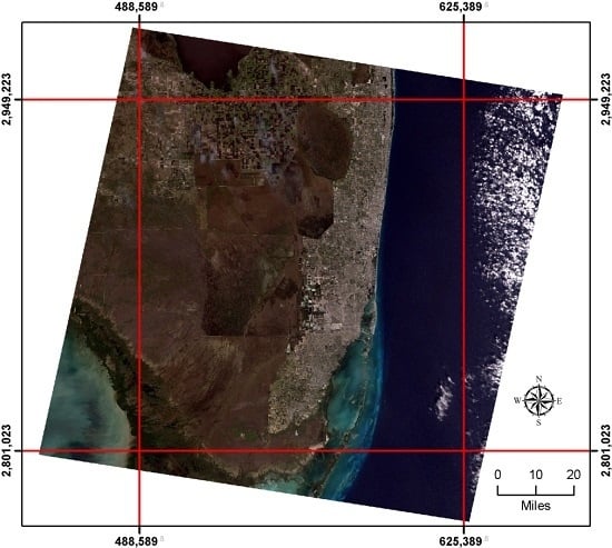
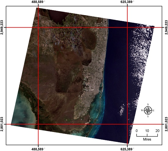
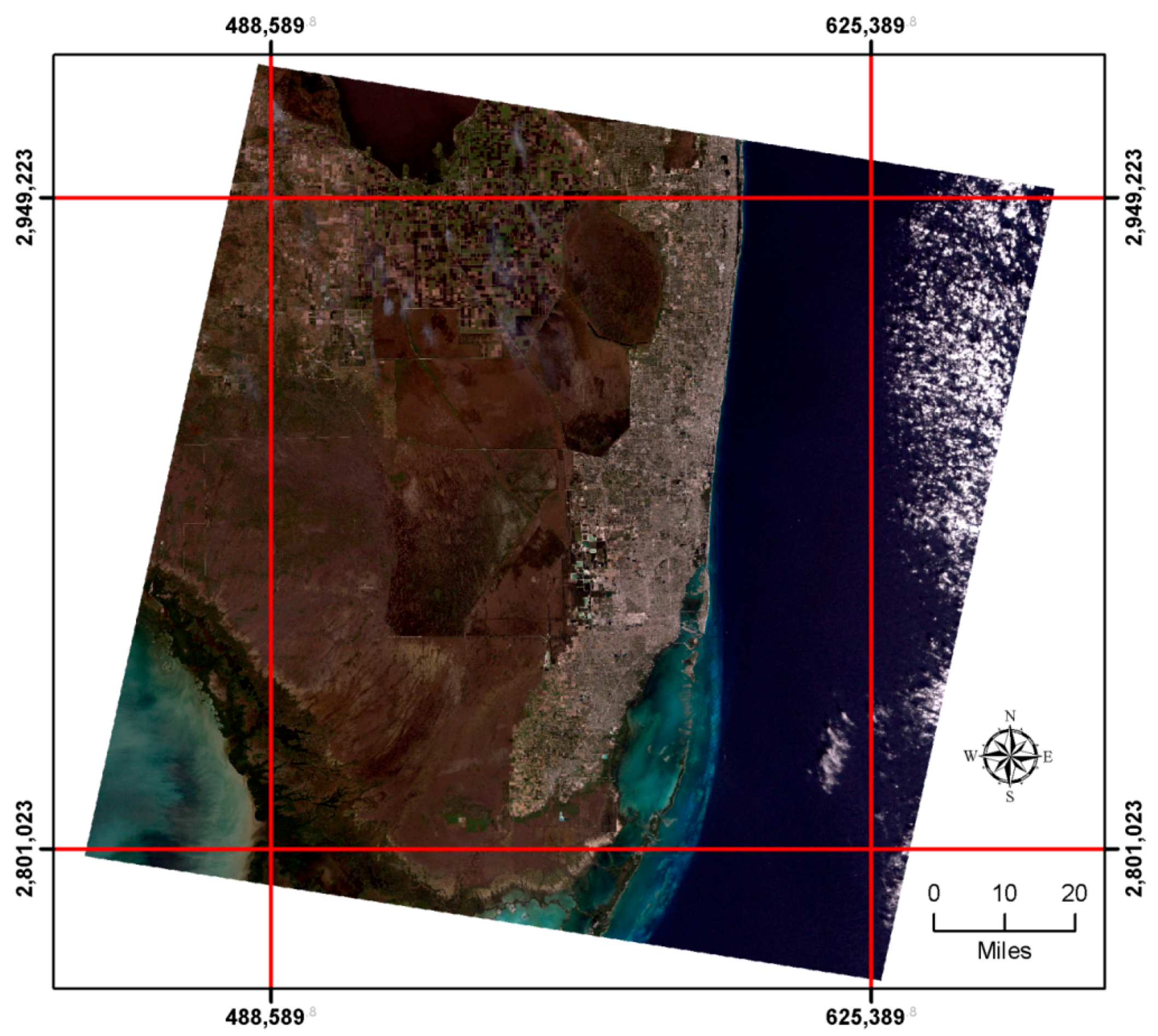
The empirical dataset employed for illustrative purposes in this paper is a 1 January 2002 Landsat 7 Enhanced Thematic Mapper Plus (ETM+) image of the Florida Everglades forming a 7649-by-8581 (
n = 65,636,069 pixels) rectangular region rotated clockwise on the horizontal axis (
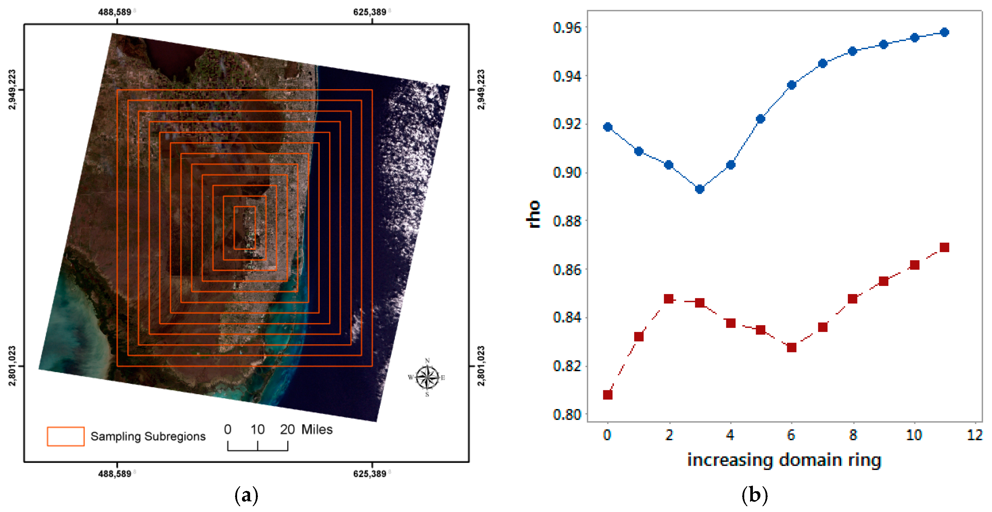
Figure 1). This image has been orthorectified and converted to the UTM 17-N projection, and includes spectral bands B1–B7; its spatial resolution is 28.5 m for bands B1–B5 and B7, and 57 m for B6 [
7]. Pixels with nonzero spectral reflectance values total 41,611,007 (82.38%), whereas 8,935,349 pixels with a zero value (17.68%) form a white border around the remotely-sensed image.
To simplify the sampling experiments whose results are summarized in this paper, a 4800-by-5200 (
n = 24,960,000 pixels) rectangular region parallel to the horizontal axis was extracted for analysis purposes (demarcated by red lines in
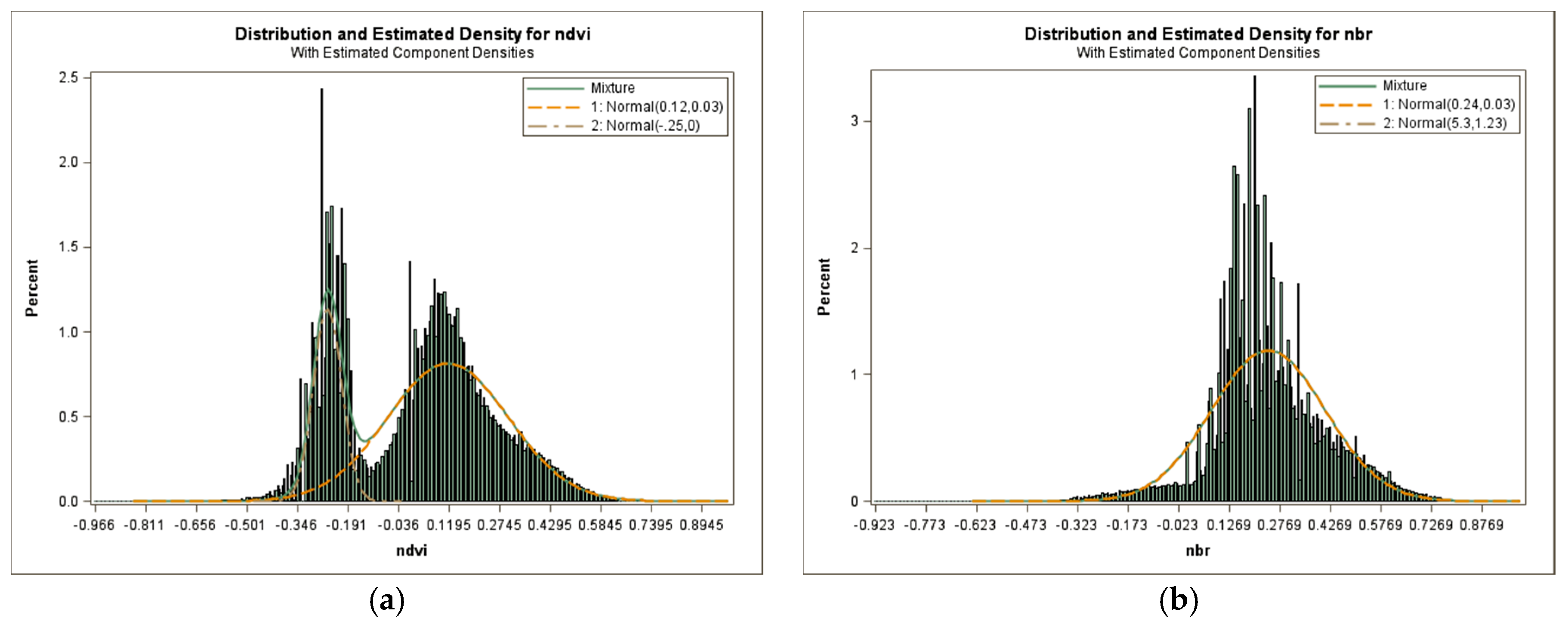
Figure 1). The sampling experiments use two spectral indices, the normalized difference vegetation index (i.e., NDVI = (B4 − B3)/(B4 + B3)) and the normalized burn ratio (i.e., NBR = (B4 − B7)/(B4 + B7)) Both indices range from −1 to 1, and have a variance that, conceptually, can range from 0 to 1. Large positive NDVI values indicate dense vegetation land cover, whereas large negative values indicate deep water. Large positive NBR values indicate high severity burn, whereas large negative values indicate high post-fire regrowth. The criterion used to select these two indices is their levels of spatial autocorrelation: NBR tends to be around 0.85 (the Everglades image analyzed in this paper has a spatial autocorrelation of 0.874), the common lower bound for many remotely-sensed images, and NDVI tends to be around 0.95 (the Everglades image analyzed in this paper has a spatial autocorrelation of 0.955), the common upper bound for many remotely-sensed images (each of these empirical results is an average of three different approximation method results).
Two of the sampling experiments whose results are summarized in this paper utilized 400-by-400 sub-regions of the Florida Everglades image; the 4800-by-5200 study region can be subdivided into 156 mutually exclusive and collectively exhaustive coterminous sub-regions of this size. Selection of this size is based upon the smaller size remotely sensed images commonly analyzed. For example, Griffith [
5] identifies a Yellowstone Park (US) image with dimensions 450-by-350 (i.e.,
n = 257,500 pixels), and an Adirondack Park (US) image with dimensions 511-by-503 (i.e.,
n = 257,033 pixels). The 400-by-400 dimensions also were utilized in the simulation experiments.
3. Spatial Regression Model Based Sampling Variability of the Spatial Autocorrelation Parameter
Spatial regression models are widely adapted to model a spatially-autocorrelated response variable. Specifically, the simultaneous spatial autoregressive (SAR) specification and the spatial autoregressive response (AR) specification are popular counterparts of linear regression under the Gaussian assumption. These specifications are utilized in this paper since distributional properties of their spatial autocorrelation parameter have been known in the literature (e.g., [
8]). This paper treats the response variable (e.g., NDVI, NBR) case of pure spatial autocorrelation, recognizing that findings can be extended to cases that include covariates (which most likely will reduce the degree of residual spatial autocorrelation). The SAR specification essentially is identical to the AR specification for pure spatial autocorrelation. This simple SAR model specification may be written as:
where
Y denotes the n-by-1 vector of response variable (e.g., NDVI, NBR) values,
is the population mean of variable Y, ρ is the spatial autocorrelation parameter (which ranges between −1 and 1 in this situation, and quantifies a signal in the data),
W is the n-by-n spatial weights matrix (i.e., a quantification of the configuration of pixels), and
ε is an n-by-1 vector of random error values (i.e., noise), which jointly are assumed to be normally distributed
. The entries in matrix
W are defined with the row-standardized rook adjacency rule: w
ij = 1/n
i if pixels
i and
j share a non-zero length common boundary, and 0 otherwise; w
ii = 0, where n
i denotes the number of neighbors pixel
i has.
Ord [
8] establishes the asymptotic variance of the maximum likelihood estimator of
(
), which furnishes the most common standard error used to evaluate estimates of this parameter. His result reduces to:
where TR denotes the matrix trace operator, superscript T denotes the matrix transpose operator, and λ
j (j = 1, 2, …,
n) denotes the eigenvalues of matrix
W (λ
1 = 1, and λ
n = −1) in descending order. If the null hypothesis is zero spatial autocorrelation, which commonly is posited, then Equation (2) reduces to:
for a regular square tessellation forming a P-by-Q complete rectangular region (e.g., a remotely-sensed image with P rows and Q columns). Equation (3) can be further re-arranged as:
a quantity that describes the variability of
regardless of whether exact eigenvalues, approximate eigenvalues, or Monte Carlo simulated eigenvalues (see
Appendix A) are used to calculate the Jacobian term or its approximation, but because of its magnitude, this quantity is of little value for quantifying uncertainty for remotely-sensed images whose
tends to be 0.85 to 0.95, or more. Rather, it suggests that the large sample sizes associated with remotely-sensed data render rather precise
s: if
for a 400-by-400 image, then 95% of the time ρ should be contained in the interval [0.943, 0.957].
The spatial autocorrelation parameter can be transformed to the range
. This transformation results in a random variable (RV) that exhibits many properties of an overdispersed beta random variable (BRV), which is defined with two parameters α and β (which appear as exponents in the BRV probability density function, and control the shape of its frequency distribution). Simulation experiments suggest that the parameters α and β of this BRV are such that
, the number of pixels (i.e., the sample size), and more specifically that
and
,
, with
(i.e., the percentage of a sample size) increasing as spatial autocorrelation increases from −1 to 1. The parameter
governs the sampling variability for a given nature and degree of spatial autocorrelation, constituting the source of overdispersion. Since it is equivalent to a percentage, p also has many properties of a BRV. The parametric mixture yields a beta-beta random variable (BBRV). Equation (4) allows the beta distributional parameters for
to be calibrated:
and
for a 400-by-400 image (the value 80,512 was calculated by equating the theoretical variance for ρ = 0 with the BBRV variance, and then solving for the single BBRV parameter).
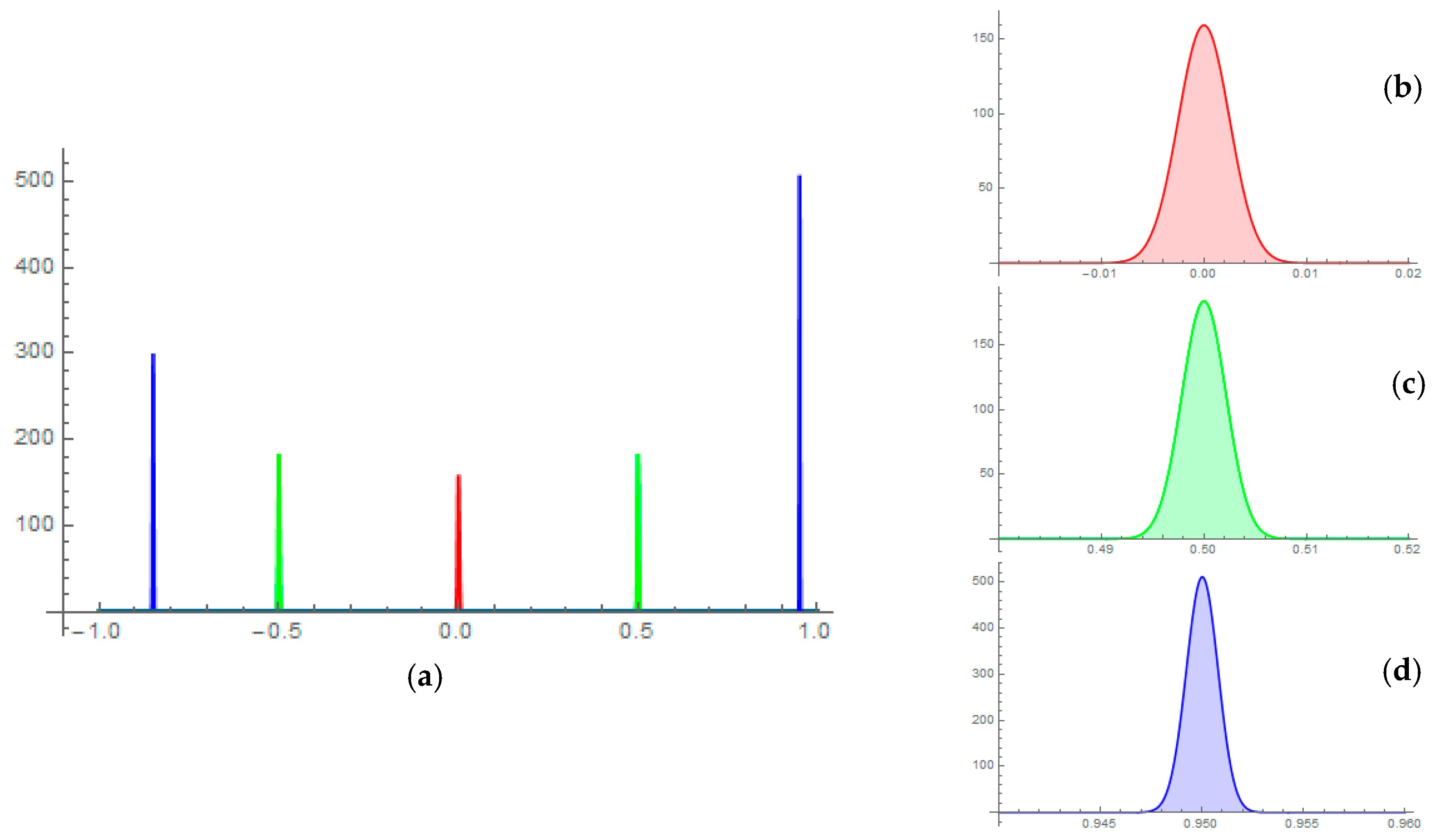
Figure 2 furnishes example sampling distributions for the specimen 400-by-400 image size studied in this paper, for ρ = −0.85, −0.5, 0, 0.5, and 0.95. Variation in height in these distributions (
Figure 2a) indicates the shrinking variance with increasing
. For example, for ρ = 0.95, a high concentration of
results in the tallest height of the distribution among the five levels.
Figure 2b–d portray zoom-ins of the sample sampling distributions for ρ = 0, 0.5, and 0.95.
Table 1 summarizes selected statistics for these types of distributions. These tabulated results corroborate the BBRV specification: the sampling distribution average equals the population parameter; the extra-beta variation is accounted for; negative skewness attributable to the upper bound of 1 exists, and positive skewness attributable to the lower bound of −1 exists; and, peakedness equivalent to that for a normal curve is present. Consequently, sound asymptotic standard errors can be calculated for any size remotely sensed image with this BBRV approximation; all that is needed is n and the value from Equation (4).
Results reported in this section allow statistical significance testing to be undertaken with regard to repeated sampling. This would be equivalent to acquiring simultaneous multiple images of the same section of the Earth’s surface. In practice, it would be roughly equivalent to, say, hourly or daily images of the same section of the Earth’s surface. Not surprisingly, these standard errors are extremely small for realistically-sized remotely-sensed images, ranging between 0.0009 and 0.0035 (
Table 1) for the 400-by-400 dimensions treated in this paper. Most likely, this is not the primary type of uncertainty that is of interest to spatial scientists and other remote sensing researchers.
4. Sampling Experiment Designed Based Sampling Variability of the Spatial Autocorrelation Parameter
The preceding section addresses model-based inference for . Its uncertainty quantification weakness is that it furnishes a measure of precision for estimates using repeated images for the same Earth surface region (the population, with a single remotely-sensed image constituting a sample from this population). However, spatial scientists and researchers often are concerned about whether or not the same value of would be obtained if its estimation employs different P-by-Q size images, ones that may or may not overlap.
Three sampling experiments were designed to quantify the variability of across a geographic landscape, and then implemented with the Florida Everglades remotely-sensed image. The first sampling experiment partitions the 4800-by-5200 pixels image into 156 mutually exclusive and collectively exhaustive 400-by-400 sub-regions. The second experiment involves a randomly selected set of 156 400-by-400 sub-regions that were allowed to overlap. The third experiment involves increasing domain sampling, and began with an 400-by-800 central set of pixels, and successively increased them by 200 pixels in each of the four directions (i.e., 800-by-1200, 1200-by-1600, …, 4800-by-5200), resulting in 12 estimates.
4.1. Coterminous Samples
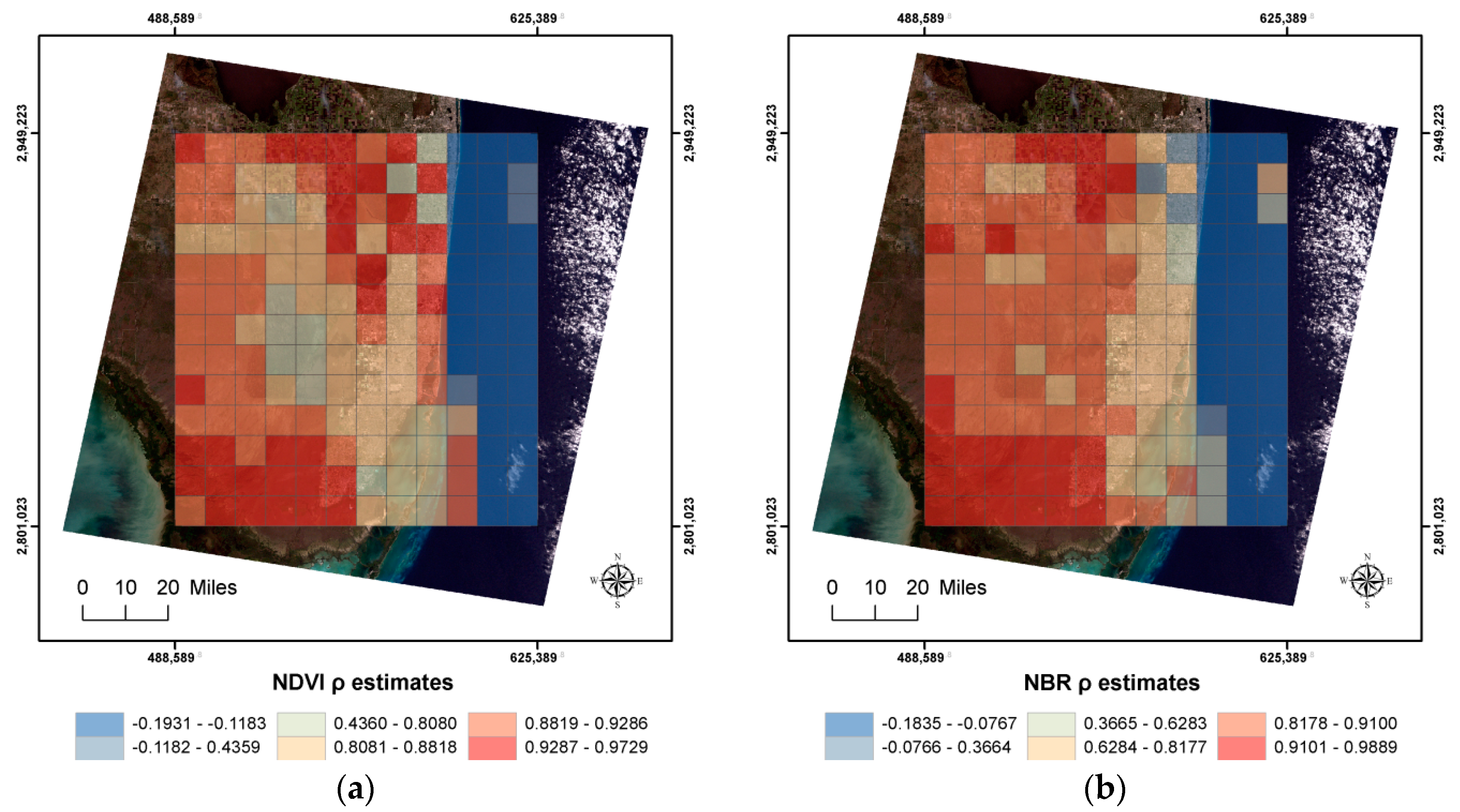
The 4800-by-5200 Florida Everglades geographic landscape was divided into 12-by-13 (i.e., 156) mutually exclusive and collectively exhaustive 400-by-400 sub-regions.
Figure 3 depicts the geographic distributions of the
s across these sub-regions.
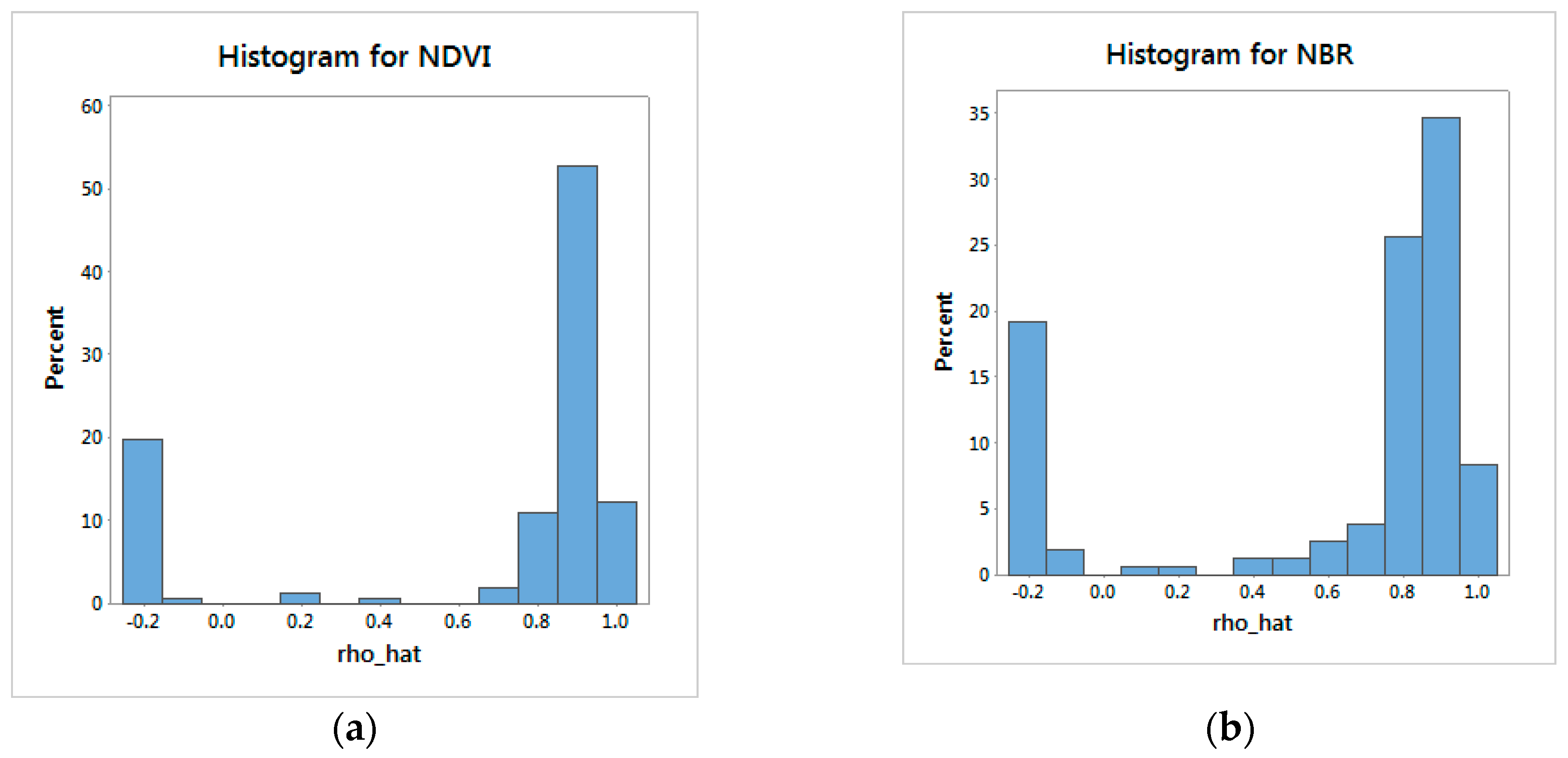
Figure 4 and
Figure 5 indicate that the image contains two different populations: land and ocean (
Figure 1). The ocean yields negative spatial autocorrelation: 32 sub-regions for NDVI, and 33 sub-regions for NBR. The respective
averages are 0.66 and 0.62, substantially less than their image-wide counterparts (Only 0.23% of the rook’s adjacency connections are lost by analyzing the 156 sub-regions. The sub-region means display moderate-to-strong positive spatial autocorrelation: for NDVI, Moran Coefficient (MC) = 0.83, and Geary Ratio (GR) = 0.12, which indicate strong positive spatial autocorrelation; for NBR, MC = 0.68, and GR = 0.25, which indicate moderate-to-strong positive spatial autocorrelation). The respective standard errors are 0.03511 (
) and 0.03422 (
), substantially greater than their model-based counterparts. These results may be inflated because this sampling experiment is similar to cluster sampling. But each sub-region being the same size removes one source of bias in cluster sampling. Because of the mixture of two populations (landscape wide, this is conspicuous for the NDVI values, but not for the NBR values;
Figure 5), this uncertainty quantification is unhelpful: the landscape-wide NDVI
is not in the 95% confidence interval [0.591, 0.729], and the landscape-wide NBR
is not in the 95% confidence interval [0.553, 0.687]. This approach also is impractical because so many subregions would need to be analyzed in order to obtain this quantification.
Restricting attention to the positive
values, the respective estimates are 0.88 and 0.83, which are much closer to their landscape-wide counterparts. In addition, the sampling variance also decreases, with respective standard errors becoming 0.00976 and 0.01268. These latter values are much closer to their model-based counterparts, but are still noticeably greater than roughly 0.0006. A spatial scientist or other remote sensing researchers may find the 95% confidence intervals, 0.931 < ρ < 0.969 for NDVI (i.e., markedly strong positive spatial autocorrelation) and 0.805 < ρ < 0.855 for NBR (i.e., strong positive spatial autocorrelation), helpful because their respective landscape-wide spatial autocorrelation parameter values are such that NDVI’s falls into its interval, and NBR’s is close to its interval. This uncertainty quantification also allows ocean results to be differentiated from land results, but remains impractical because so many sub-regions would need to be analyzed in order to obtain it. The challenge that remains is to be able to compute these standard errors analytically, perhaps with guidance from cluster samples sampling theory (The
s are an inverse function of their subregion standard deviations, a specification that offers a way to establish a random variable whose variance may be useful here (see [
9])).
4.2. Random Subregion Samples
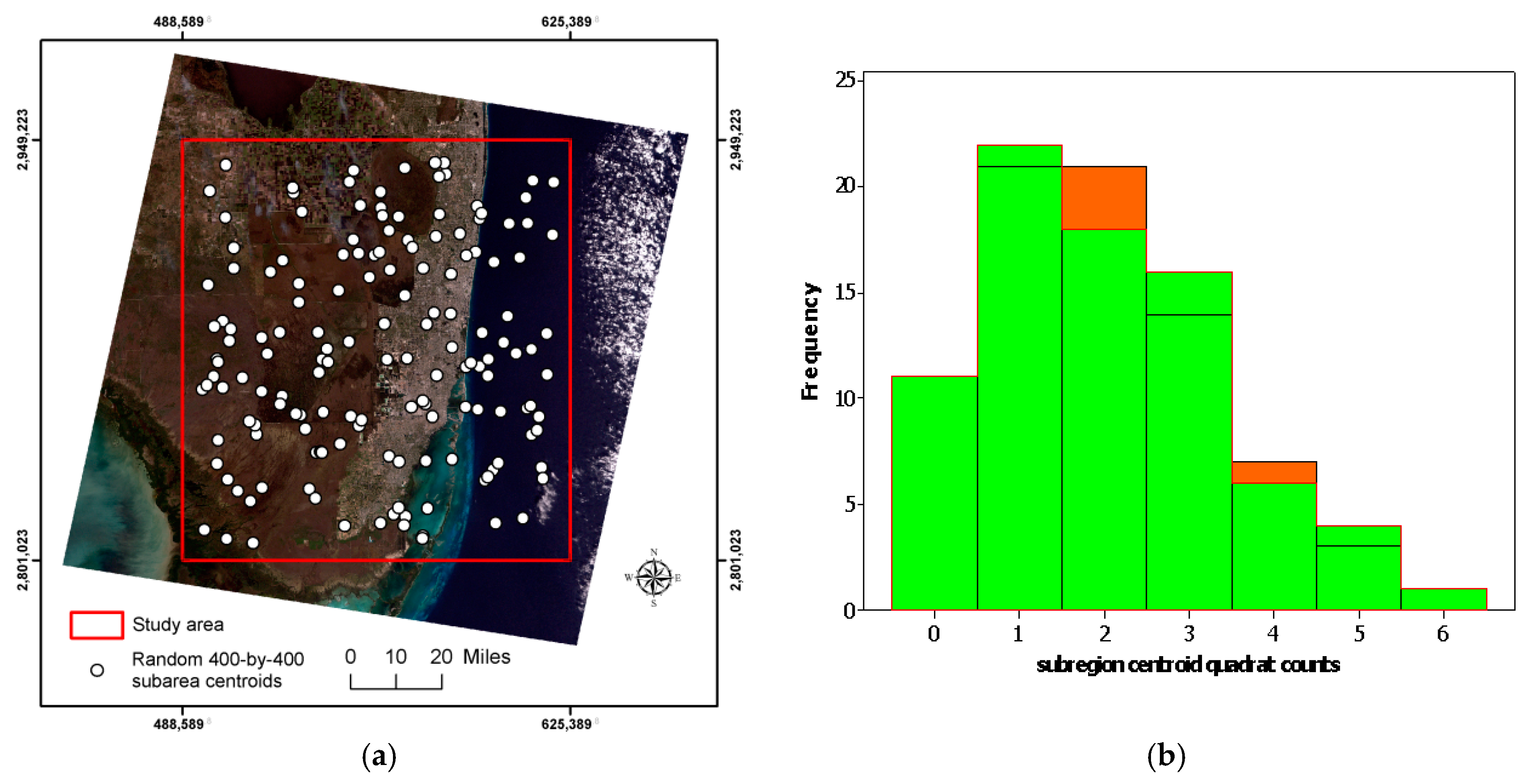
Next, 156 random sub-regions were selected, such that their centers came from the central 4400-by-4800 sub-region of the Florida Everglades image, which is defined by the southwest coordinate (2101, 1401) and the northeast coordinate (6500, 6200). The UTM coordinates for the southwest and northeast corners are (494,289.8, 2,806,723) and (619,689.8, 2,943,523), respectively.
Figure 6a portrays the geographic distribution of the centroids of these sub-regions; their spacing/density distribution is a Poisson RV (
Figure 6b). The ocean yields negative spatial autocorrelation: 24 random sub-regions for NDVI, and 27 random sub-regions for NBR. The respective
averages are 0.69 and 0.64, respectively, very similar to their coterminous quadrat counterparts. The respective standard errors are 0.03203 (
) and 0.03162 (
), again very similar to their coterminous quadrat counterparts, and substantially greater than their model-based counterparts.
Restricting attention to the positive values, the respective estimates are 0.85 and 0.81, which are much closer than equivalent coterminous quadrat values to their landscape-wide counterparts. In addition, the sampling variance also decreases, with respective standard errors becoming 0.0320 and 0.0316. These means are much closer to their model-based counterparts, but these standard deviations are noticeably greater than their coterminous quadrat counterparts. A spatial scientist or other remote sensing researchers may find the 95% confidence intervals, 0.824 < ρ < 0.876 for NDVI and 0.787 < ρ < 0.833 for NBR, less helpful because neither landscape-wide spatial autocorrelation parameter value falls into its respective interval. This uncertainty quantification seems less useful than the preceding coterminous quadrat based one. Therefore, the challenge appears to be designing an analytical method to compute standard errors relating to mutually exclusive and collectively exhaustive coterminous quadrat sub-regions.
Removing the coterminous constraint on the data, an experiment was performed involving 156 samples of size 160,000, where the sample pixels were randomly selected from the set of 24,960,000 pixels with equal probability but without replacement; the spatial lag term was calculated with the four surrounding pixels, and hence was selected as part of a bivariate sample. The Jaocbian term is not correct here. Nevertheless, the average s obtained with ordinary least squares (OLS) are 1.006 and 0.995, respectively, for NDVI and NBR; the first is not a feasible value (not only does this arithmetic average exceed 1, but all 156 estimates exceed 1). Retaining the original Jacobian term yields, respectively, s of 0.958 and 0.869 (these equal their respective estimates for the full 4800-by-5200 image). Their corresponding standard errors are 0.00056 and 0.00105, which, again, suggests that repeated sets of 156 random samples of size 160,000 will yield sound complete image parameter estimates.
Consequently, random sub-regions furnish useful measures of uncertainty, but random pixels do not. Unfortunately, in practice, such repeated sampling places a considerable data collection and computational burden on a spatial analyst. Once more, the challenge that remains is to be able to compute these standard errors analytically, again perhaps with guidance from cluster samples sampling theory.
4.3. Increasing Domain Subregions
A third possible approach to quantifying uncertainty of
is to study how this estimate changes with increasing geographic landscape size (i.e., scale;
Figure 7a).
Figure 7b portrays the change in the Everglades NDVI and NBR
s with an increasing domain. Their respective unweighted averages are 0.929 and 0.842 (
Table 2), again indicating some bias. Meanwhile, their respective standard errors are 0.02353 and 0.01635, which are smaller than those obtained with coterminous or random cluster sampling. These standard errors are still substantially larger than their counterpart values furnished by Equation (4).
Therefore, an increasing domain furnishes somewhat useful measures of uncertainty. Unfortunately, in practice, this approach also places a considerable data collection and computational burden on a spatial analyst. As before, the challenge that remains is to be able to compute these standard errors analytically.
6. Conclusions and Implications
Uncertainty associated with remotely-sensed data should be cast in terms of its latent spatial autocorrelation, denoted here by . Since this measure tends to be in the range [0.85, 0.95] for most remotely-sensed data, it indicates that these data contain considerable redundant information which, in turn, means the presence of substantial VIFs. The standard method of quantifying any additional uncertainty introduced by estimating ρ appears to be negligible, as indicated by Equation (4) for ρ = 0 (which essentially is irrelevant for remotely sensed data), and indicted by both Equation (3) and the BBRV mixture proposed in this paper for .
Most geographic landscapes suggest that Equation (3) fails to furnish an adequate quantification of uncertainty for ; its variability in a geographic landscape is substantially greater than values produced by Equation (3). The various analyses summarized in this paper for the Florida Everglades remotely-sensed image corroborate this contention. This inconsistency arises from the inferential basis for Equation (3): repeated images of the same region of the Earth’s surface. Treating different regions introduces another source of variability into . This is the uncertainty of interest to most spatial analysts. Would a slightly larger/smaller image, an image shifted slightly to the east and/or north, or an image from a different part of a larger geographic landscape yield essentially the same ? The variability detected in analyses summarized in this paper reveals quantities many times larger than those rendered by Equation (3).
The remaining challenge is to formulate an analytical specification of this type of variability. Evidence presented in this paper suggests that cluster sample sampling theory may furnish insights into what this specification should be. The final formula should be a function of , the variance of the spectral index being studied, the variance of the spatial autocorrelation filtered data (i.e., what is equivalent to independent and identically distributed values), and the sample size, n. Establishing such a formula will support a better extraction of information and distilling of knowledge from remotely-sensed data by, especially, accounting for their latent spatial autocorrelation.
Finally, spatial regression should be utilized in studies that utilize remote sensing data. Regression is extensively used to model various phenomena such as land use and land cover [
4,
11], NDVI [
12,
13], urban heat island [
4], and landslide susceptibility [
14], but spatial autocorrelation has been barely accommodated in modeling remotely-sensed data. Remotely-sensed data has a strong positive spatial autocorrelation in most cases: even one with a fragmented (e.g., land use) pattern with a coarse resolution (e.g., 250 m of MODIS). Ignorance of spatial autocorrelation can result in unreliable results.


