An IPCC-Compliant Technique for Forest Carbon Stock Assessment Using Airborne LiDAR-Derived Tree Metrics and Competition Index

Abstract

This study developed an IPCC (Intergovernmental Panel on Climate Change) compliant method for the estimation of above-ground carbon (AGC) in forest stands using remote sensing technology. A multi-level morphological active contour (MMAC) algorithm was employed to obtain tree-level metrics (tree height (LH), crown radius (LCR), competition index (LCI), and stem diameter (LDBH)) from an airborne LiDAR-derived canopy height model. Seven biomass-based AGC models and 13 volume-based AGC models were developed using a training dataset and validated using a separate validation dataset. Four accuracy measures, mean absolute error (MAE), root-mean-square error (RMSE), percentage RMSE (PRMSE), and root-mean-square percentage error (RMSPE) were calculated for each of the 20 models. These measures were transformed into a new index, accuracy improvement percentage (AIP), for post hoc testing of model performance in estimating forest stand AGC stock. Results showed that the tree-level AGC models explained 84% to 91% of the variance in tree-level AGC within the training dataset. Prediction errors (RMSEs) for these models ranged between 15 ton/ha and 210 ton/ha in mature forest stands, which is equal to an error percentage in the range 6% to 86%. At the stand-level, several models achieved accurate and reliable predictions of AGC stock. Some models achieved 90% to 95% accuracy, which was equal to or superior to the R-squared of the tree-level AGC models. The first recommended model was a biomass-based model using the metrics LDBH, LH, and LCI and the others were volume-based models using LH, LCI, and LCR and LDBH and LH. One metric, LCI, played a critical role in upgrading model performance when banded together with LH and LCR or LDBH and LCR. We conclude by proposing an IPCC-compatible method that is suitable for calculating tree-level AGC and predicting AGC stock of forest stands from airborne LiDAR data.

1. Introduction

Estimating above-ground carbon (AGC) stock in dense forest normally involves conducting a ground-based inventory and logging sample trees from multiple forest plots. Tree parameters (such as diameter and height) are then correlated in an allometric model to estimate individual tree volume/biomass or carbon stock. Calculations for stand-level AGC are based on a stand structure model of tree diameter and height distribution. Parameters are fitted into a probability distribution function in order to estimate the AGC for an entire forest stand [1,2]. Although conventional techniques provide reasonably accurate estimates of volume, biomass, and forest stand carbon stocks, field-inventory-based methods are often labor intensive and can require time-consuming measurements and inspections. Field inventories also lack detailed information concerning variations in the canopy structure and changes in the wider forest ecosystem. The use of remote sensing, especially LiDAR remote sensing technology partly overcomes these limitations.

LiDAR data has been increasingly applied to the collection of forest data. Several methods of estimating forest volume/biomass using airborne LiDAR [3,4,5,6,7,8,9,10,11] and satellite-based LiDAR metrics [12,13,14,15,16] have been developed. In brief, methods for estimating the volume, biomass, and/or AGC can be characterized as plot-based and tree-based approaches. Plot-based approaches generally use the average height of trees in a stand [9,10], or mean canopy profile height [11], which can be obtained from a high or low-resolution LiDAR-based canopy height model (CHM). Generally, estimates obtained using plot-based averaging techniques lack precision due to the uncertainty caused by forest structure variations within the forest space [2,17,18,19,20,21] particularly when the forest covers a large geographical scale area. As Bombelli et al. [22] states, “In situ measurements can generally measure biomass with accuracy from 20% to 2%, depending on the geographical scale.” This kind of measurement error can be reduced by increasing the number of sample plots measured in the physical forest inventory, especially, if representative plots can be collected from all the various trees species in the forest. However, stand parameters, such as the height of dominant and co-dominant trees occupying the overstorey of a forest stand, can change dramatically due to variations in terrain. Additionally, tree proportions may change significantly due to competition between individual trees in a forest stand. Thus, variations in forest structure and changes within the forest space can lead to a reduction in the accuracy of AGC stock estimation in the sample plots [2].

Recently, a few studies have attempted to improve the accuracy of stand-level volume estimates and above-ground biomass and carbon estimates by combining LiDAR data with multi-frequency radar data [23] or medium-high resolution satellite data [24]. These algorithms offer a reasonable method for gathering general information on forest stands, but lack the precision of tree-level allometric equations, which are based on specific tree characteristics and can significantly improve the accuracy of volume/biomass/carbon estimation [1,2,25]. Individual tree-level data can be obtained either directly or indirectly from high-density airborne LiDAR data and some examples can be found in [26,27,28,29,30,31,32,33,34].

The use of individual tree-level parameters such as tree diameter, usually measured at the breast height (DBH), and tree height (H) offers a more precise method of estimating tree volume in forest allometry. These parameters are generally incorporated into nonlinear models, such as the Schumacher-Hall formula to determine tree volume. While tree height may be obtained directly from the airborne LiDAR data, DBH must be calculated using LiDAR-derived metrics. In addition to the height, crown diameter and crown geometric volume, a new index that accounts for a tree’s spatial relationship with its neighbors, the growth competition index, has been demonstrated to be an important controlling factor in deriving DBH and estimating volume from a LiDAR model [34].

The forest ecosystem is the largest carbon sink in the terrestrial ecosystem; however, the forest ecosystem can become one of the largest sources of carbon due to emissions released as the result of deforestation and forest degradation due to anthropogenic activities. The strengthening global effort to reduce carbon emissions has resulted in greater consideration of the financial value of the carbon stored in forests. This has become known as Reducing Emissions from Deforestation and Forest Degradation (REDD+) [35]. It is imperative that a protocol be established to account for changes in forest resources and accurately assess national carbon credits. According to the IPCC (Intergovernmental Panel on Climate Change) [36], the living biomass carbon stock of individual trees in a forest stand can be determined as the product of tree volume (V), wood density (D), biomass expansion factor (BEF), and carbon fraction (CF). Although remote sensing has been intensively used to estimate forest biomass, rarely has research explored the issue by combining remote sensing LiDAR data with the IPCC method of estimating AGC. Therefore, the objectives of this paper are: (1) To develop a range of tree-level AGC estimation models using LiDAR-derived tree metrics with respect to the IPCC protocol; and (2) To measure the effectiveness of the range of tree-level AGC models in predicting stand-level forest carbon stocks and determine an appropriate algorithm for practical use in stand-level AGC stock accounting.

The first step of the proposed protocol applied the multi-level morphological active contour (MMAC) algorithm to a LiDAR derived CHM image of the study area. The algorithm identifies and delineates individual tree crowns in dense forest based on rasterized airborne LiDAR data. Tree size parameters, such as tree height and crown radius were directly derived and the competition index and diameter at breast height were indirectly derived for each tree in the plot from the CHM image. A model was then developed for estimating individual tree AGC using various combinations of these tree-level parameters. After that, the entire forest stand AGC was calculated by summing the AGC estimates for each individual tree in the forest stand. The performance of the models was assessed based on comparison with previously acquired ground-based inventory observations and the IPCC-method for calculating AGC stock values.

2. Material and Methods

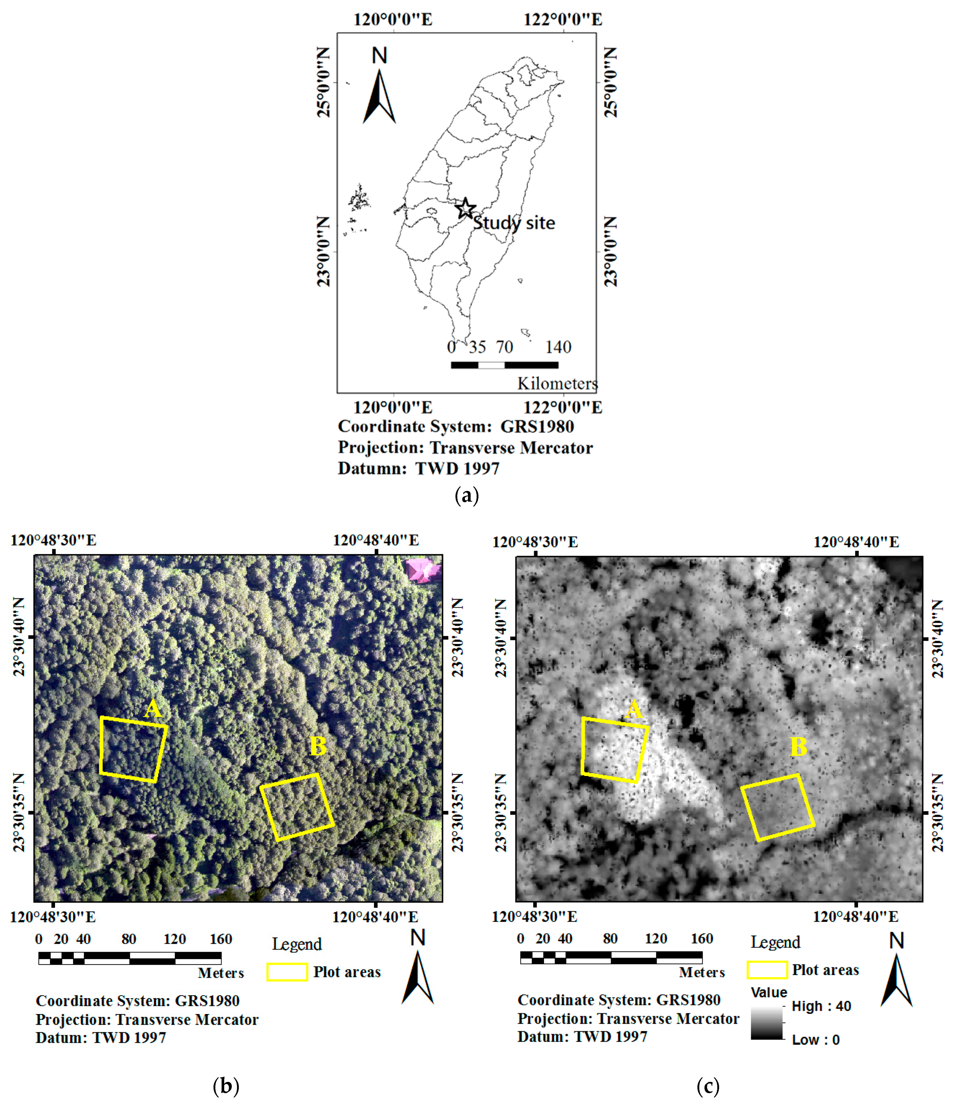
2.1. Airborne LiDAR Data Collection

Alishan National Forest, centered at 23°30′N, and 120°48′E in southern Taiwan, provided the location for this study. Ground elevation ranged between 2000 and 2500 m above sea-level. Airborne LiDAR data was acquired on 20 April 2007 via Eagle Forestry Service (EFS) Technologies using a BN-2 Islander plane. A small-footprint, multi-return LiDAR system (Leica-Geosystems ALS50) mounted on the plane provided high-accuracy digital surface data. Up to four returns were recorded per laser pulse. LiDAR data was collected at an operating flight altitude of 10,000 feet, the pulse rate was 40.9 KHz, and the scan rate was 17 Hz, FOV was 37 degrees. These settings produced footprints approximately 0.4 m in diameter across an average swath width of 473 m. Following boresight calibration, the LiDAR datasets had 15 cm and 2.2–20 cm of xy- and z-accuracy. LiDAR datasets with canopy pulse return densities of 5.21 returns per m² were then used to produce a rasterized digital surface model (DSM) and digital elevation model (DEM) using a linear interpolation technique (0.40 m cell resolution). The CHM was calculated by subtracting the DEM from the DSM as described in Lin et al. [37] using a TerraScan system.

2.2. Datasets Used to Train and Validate the AGC Models

The training dataset for the tree-level AGC models consisted of an inventory dataset of 35 trees and was entirely separate from the validation dataset. This training dataset contained both in situ measured tree size parameters and LiDAR CHM-derived metrics. Each of the trees within the training sample was easily identifiable both by manual inspection in situ and in the CHM image. The same dataset had been used previously to model individual tree-level stem diameter and stem volume by Lo and Lin [34].

The validation dataset for the tree-level AGC models consisted of a conifer stand comprised of two species, Taiwan red cypress (Chamaecyparis Taiwanensis Matsum.) and Japanese cedar (Cryptomeria japonica D.Don). The two 0.25-hectare plots (Figure 1a,b) had been used previously in the development of the MMAC technique [37] and in the development of tree volume estimation models [34]. The Japanese cedar and Taiwan red cypress plantations in plot A and plot B were regenerated in 1914 and 1920, respectively.

A ground-based inventory recorded the following measurements for every tree in the two validation plots: diameter at breast height, tree height, and crown width. Tree volume was calculated. Inventory data were collected in a series of projects sponsored by the Taiwan Forestry Bureau between 2006 and 2008. The number of trees in the plots of Japanese cedar and Taiwan red cypress plots was 101 and 116, which is equal to a stand density of 632 and 725 trees per hectare respectively. On average, Japanese cedar DBH of 64.60 ± 13.34 cm was larger than the Taiwan red cypress DBH of 36.70 ± 7.65 cm, and the average Japanese cedar height exceeded that of the Taiwanese red cypress at 29.43 ± 2.58 and 21.39 ± 1.89 m respectively. As a consequence of previous experiments [38], the wood density, biomass expansion factor, and carbon fraction of Japanese cedar and Taiwan red cypress were determined to be 0.51, 1.23, 0.50 and 0.50, 1.24, 0.50, respectively. According to the IPCC method (Equation (1)), the AGC of the trees in the training sample can be determined using allometric formula (Equations (2) and (3)) for the two tree species. Allometric formulae for Japanese cedar and Taiwan red cypress respectively are shown in Equations (2) and (3), respectively.

$$AGC=AGB\times CF=V\times D\times BEF\times CF$$

(1)

$$AGC=0.51\times 1.23\times 0.5\times (0.0000902DB{H}^{1.9886}{H}^{0.6879})$$

(2)

$$AGC=0.50\times 1.24\times 0.5\times (0.0000944DB{H}^{1.9947}{H}^{0.6597})$$

(3)

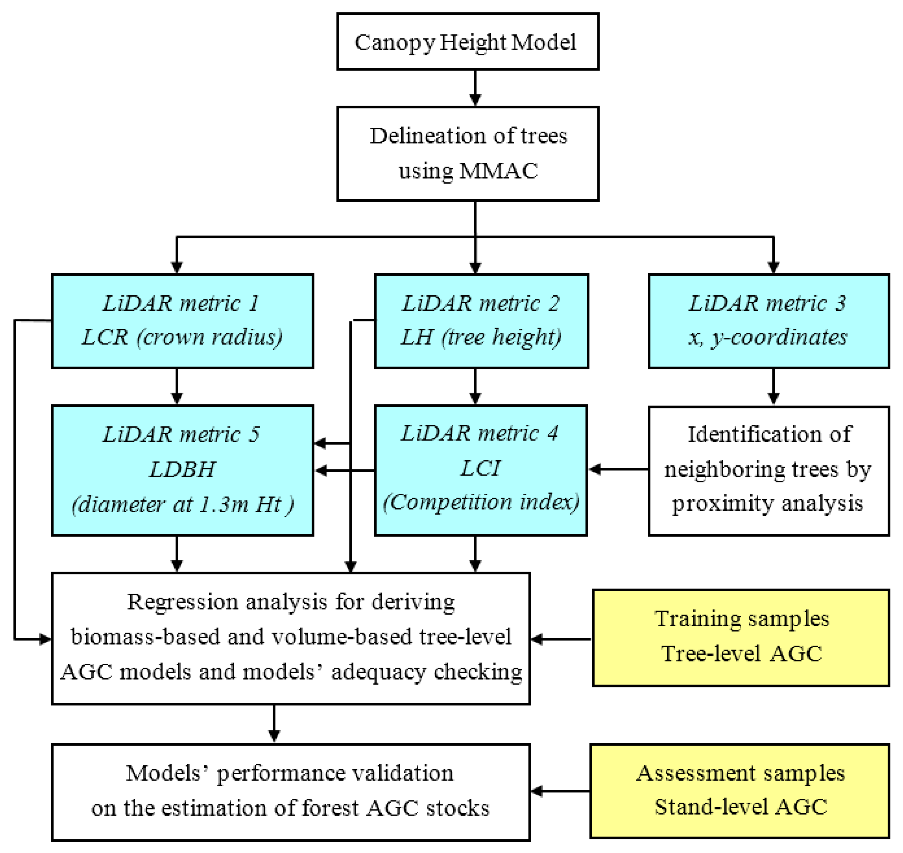
2.3. A Tree-Level Algorithm to Account for Above-Ground Carbon

Figure 2 presents a flowchart showing the protocol followed in this study. In contrast to the local-maxima-filtering techniques and tree-model-based techniques, the determination of window size and tree-shape parameters are not required a priori. The MMAC technique [37] incorporates mathematical morphology to locate the position of each tree stem candidate and then delineates the crown outline. It was developed to delineate trees in mountainous mature forest where competition between individual trees is significant and causes the size of tree parameters to vary dramatically, particularly in dense mature forest stands. Firstly, the tree-level LiDAR parameters were extracted from the rasterized CHM image using the MMAC algorithm. These parameters were tree height (LH), crown radius (LCR), and the location of each tree. Secondly, proximity analysis was carried out using a fixed radius of 20 meters from a subject tree to identify neighboring trees and determine the tree’s competition index (LCI). Thirdly, a regression analysis was applied to derive appropriate models for estimating the DBH of trees (LDBH) using the previous metrics. Fourthly, the inventoried AGC of trees was regressed on the LiDAR-derived tree metrics in the training dataset to obtain empirical tree-level AGC models. Finally, the tree-level AGC models were validated by measuring their performance in predicting above-ground carbon for the forest stand using the assessment dataset.

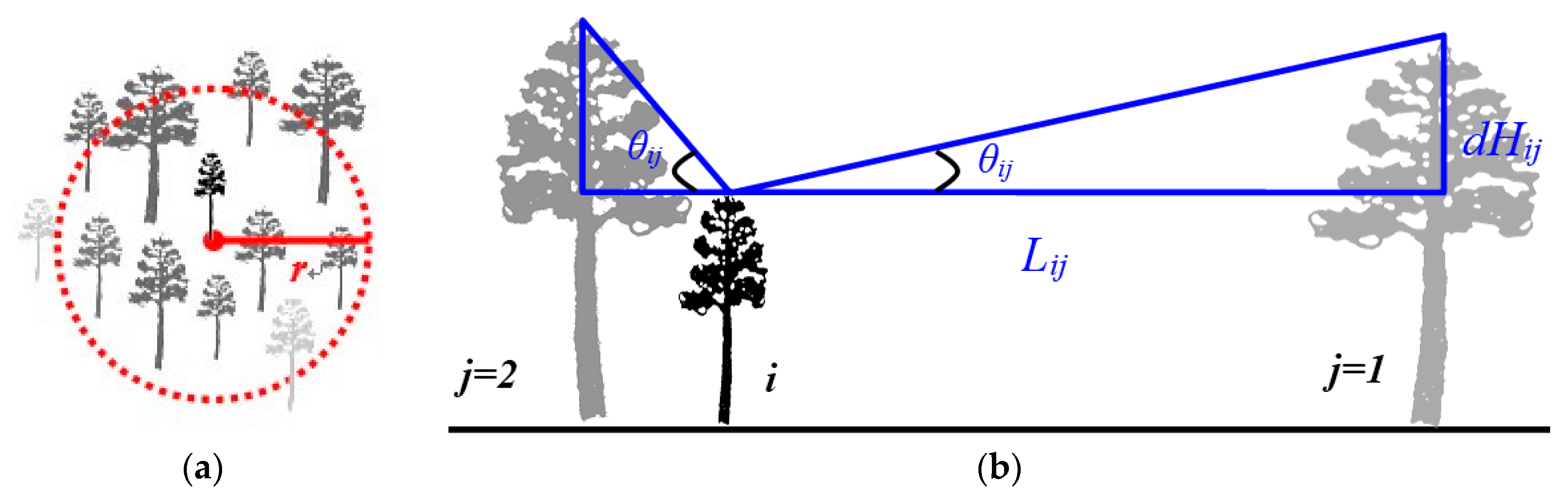
2.3.1. LiDAR Derived Tree-Level Parameters

Lin et al. [37] found the MMAC algorithm to be a practical means of detecting and delineating individual trees in mature forest using a LiDAR-derived CHM image. The individual tree parameters that were derived using the MMAC algorithm were: total height, precise location, and crown radius. In summary the MMAC algorithm operates as follows: Firstly, a bottom-up erosion (BUE) technique locates all the tree candidates in the sample area. A refining erosion process then moves upwards from the minimum value in a CHM image (the lowest dark gray level in the image) to the maximum value in a CHM image (the lightest gray level in the image). All tree candidates (the local maxima points determined without the disadvantage of window-based filtering methods) are then revealed. Each tree candidate is referred to as “a seed blob” and is the apex of a tree, usually a single point or an irregularly shaped region. The pixel with the maximum value in a seed blob has a specific coordinate (x, y) and represents the center location of a tree. Its value is directly LiDAR-derived, and equivalent to the tree height, LH, measured in meters; Secondly, a top-down dilation (TDD) technique estimates the tree crown periphery points by growing outwards from the seed blob of a tree candidate. This dilation process ceases when the circularity of the dilated shape exceeds a specified threshold or the value of adjacent pixels indicates a sudden variation in height. These criteria ensured a reasonable degree of roundness in the shape of the tree crown and prevented the tree crown edge from over-shooting its maximum permissible proportions. Finally, an active contour model (ACM) modified the periphery points to delineate the precise contours of the tree crown boundary. This step provides a feasible estimate for the boundaries of the tree crown and the crossover points between them in the case of overlapping crowns. Delineated tree crown contours were then used to determine the parameter LiDAR-derived crown radius LCR measured in meters.

Following MMAC processing, a second parameter, known as the competition index LCI was calculated from the primary parameters, LH and the x- and y-coordinates of the surrounding trees in an area. Competition is a constant and natural phenomenon occurring between individual trees and other plants within a limited parcel of forestland. In dense forest, every tree competes with its neighbors for limited resources such as light, water and space, all of which are required for growth (Figure 3a). Therefore, the level of competition for any particular tree depends on the number and the size of its competitors, and its proximity to other trees within a particular space. Competition stresses for a subject tree in a proximity area can be expressed in terms of the angles, distances, and the height differences between a subject tree and its competitors, or neighbors, in a CHM image (Figure 3b).

Assume that the small black tree in Figure 3a is the subject tree. The proximity area of the subject tree can be drawn using a radius (r) centered at the location of that subject tree. The nine dark-gray trees within the proximity perimeter are recognized as the subject’s direct competitors while the two light-gray trees located outside the boundary are not. The competition index of the subject tree ($LC{I}_i$) is determined by Equations (4)–(6) using the distance ($L_{ij}$) and the height difference ($d{H}_{ij}$) between each pair of subject ($i$) and competitor ($j=1\dots n$). Theoretically, the value of LCI ranges between zero and some positive number. A tree suffers no competition stresses whatever if its competitors are shorter in height or it grows in open land with no competitor trees inside its proximity perimeter. In general, a small radius would be inadequate in describing a tree’s competition index due to the inability to account for potential influences from adjacent tall trees. Conversely, too large a radius may include some neighboring trees, which exert no significant effect on the growth of the subject tree. Due to average tree height in this study (between 20 m and 30 m) and the prevalent conditions in the study plots, a proximity radius of 20-m was considered appropriate for this study. Following the determination of LH, LCR, and LCI, the secondary LiDAR-derived tree metric LDBH was determined by Equations (7)–(10). Correspondingly, the coefficient of determination of Types 1–4 LDBH was 0.71, 0.76, 0.82, and 0.84 and their RMSE performance in diameter estimation was 11.2, 10.1, 9.5, and 8.7 cm which equaled to an percentage RMSE of 18%, 16%, 14%, and 14% respectively [34]. Four types of LDBH were compared in the determination of AGC stocks when LDBH was derived using variant primary metrics.

$$LC{I}_i={\displaystyle \sum _{j=1}^n{\theta }_{ij}}={\displaystyle \sum _{j=1}^n{\tan }^{-1}\left(\frac{d{H}_{ij}}{L_{ij}}\right)},\text{where }{\theta }_{ij}=0\text{ if }d{H}_{ij}<0$$

(4)

$$L_{ij}=\sqrt{{[{(x,y)}_i-{(x,y)}_j]}^2}$$

(5)

$$d{H}_{ij}=h_j-h_i$$

(6)

$$Type-1LDBH:LDBH1=exp\left(1.479+0.864lnLH\right)$$

(7)

$$Type-2LDBH:LDBH2=exp\left(1.473+0.835lnLH+0.003LC{R}^2\right)$$

(8)

$$Type-3LDBH:LDBH3=exp\left(1.607+0.857lnLH-0.009LCI\right)$$

(9)

$$Type-4LDBH:LDBH4=exp\left(1.587+0.838lnLH-0.007LCI+0.002LC{R}^2\right)$$

(10)

2.3.2. Regression Analysis for Deriving Tree-Level AGC Models

Regression analysis is generally used to derive models that describe the statistical relationships between dependent and independent variables. In cases of a robust relationship, the value of a dependent variable can be accurately estimated using suitable independent variables. In forest inventory, carbon/biomass/volume of individual trees is generally expressed as a function of tree size parameters such as DBH and H in the form of allometric formula. The variables used in the formulae were collected from the ground survey data.

In order to show the value of each LiDAR-derived variable in predicting AGC, the inventoried AGC for each tree in the training dataset was regressed against the LiDAR tree metrics: LH, LDBH, LCR, and LCI in a variety of variable combinations so as to build a range of biomass-based tree-level AGC models. The models were built using a method of multiple linear regression. All the predictor variables were initially used to build a regression model. Then, a method of backward elimination was employed to remove a predictor based on its level of importance and the practicality of the allometric formula in forestry. Similarly, the inventoried tree volume was regressed on the tree metrics to build a range of tree volume models and then integrated with the scalars of D, BEF, and CF to create volume-based tree-level AGC models. In summary, the biomass-based and volume-based tree-level AGC models have the form of the Schumacher-Hall formula as expressed in Equations (11) and (12) where Xi indicates the ith LiDAR-derived tree metrics, a_i and b_i are the regression coefficients, and value of the scalars D, BEF, and CF is species-specific which is determined from inventory data and laboratory analysis.

$$\text{Biomass-based model: AGC}=a_0{\displaystyle {\prod }_{i=1}^n{X}_i^{a_i}}$$

(11)

$$\text{Volume-based model: AGC}=V\times D\times BEF\times CF=(b_0{\displaystyle {\prod }_{i=1}^n{X}_i^{b_i}})\times D\times BEF\times CF$$

(12)

2.3.3. Evaluating the Predictive Performance of the Models

Several accuracy measures were applied to evaluate model performance in order to get sufficient accuracy observations for examining the significance of accuracy differences among the developed AGC models. The root-mean-square error (RMSE) (also known as root-mean-square deviation (RMSD)) is a commonly used measure for assessing the prediction capability of algorithms. Mean absolute error (MAE) is also used to measure prediction accuracy. In forecasting, the scale indicating data range and data unit is generally considered for accuracy comparison. RMSE is on the same scale as the data and therefore theoretically relevant in modeling the variance. This makes RMSE a useful measure for comparing different methods of processing the same set of data. In Equations (13) and (14), n is the number of samples, y and $\widehat{y}$ represent the observed and predicted value respectively. While RMSE and MAE are scale-dependent measures, they are not suitable when making comparisons across data sets with different scales. However, RMSE can be expressed as a percentage deviation from the mean observation ($\overline{y}$) as shown in Equation (15). The percentage RMSE (abbreviated as PRMSE or RMSE %) is a scale-independent measure that is capable of evaluating the precision of a model’s predictive performance. Equation (16) shows another scale-independent measure, root mean square percentage error (abbreviated as RMSPE) which is a measure of average deviation from a true value. RMSPE is frequently used to compare predictive performance across different data sets [39]. Thus, the predictive accuracy of the AGC models which used LiDAR-derived tree-level metrics to estimate forest AGC stocks was evaluated using four performance indices: MAE, RMSE, PRMSE, and RMSPE. Note that a model with a smaller index value has a superior AGC prediction performance.

$$MAE=\frac{1}{n}\left[{\displaystyle \sum _{i=1}^{n}abs({\widehat{y}}_i-y_i)}\right]$$

(13)

$$RMSE=\sqrt{\frac{1}{n}{\displaystyle \sum _{i=1}^n{({\widehat{y}}_i-y_i)}^2}}$$

(14)

$$PRMSE=\left(\sqrt{\frac{1}{n}{\displaystyle \sum _{i=1}^n{({\widehat{y}}_i-y_i)}^2}}/\overline{y}\right)\times 100\%$$

(15)

$$RMSPE=\sqrt{\frac{1}{n}{\displaystyle \sum _{i=1}^n{\left(\frac{{\widehat{y}}_i-y_i}{y_i}\right)}^2}}\times 100\%$$

(16)

Lin and Dugasuren [40] introduced a percentage change index to account for spatiotemporal vegetation productivity. The same method can be applied to the AGC models to show how well alternative models contributed to stand-level AGC estimation relative to a base model. We assume that the least accurate tree-based AGC model can be regarded as the base model. Let S be the accuracy achieved by the base model and X be the accuracy of an alternate model, then the accuracy improvement percentage (AIP) of the alternate model can be determined using Equation (17).

$$\text{AIP}=\left(X-S\right)/S\times 100\%$$

(17)

Since X − S represents any improvement in accuracy over the base model, AIP can transform the MAE, RMSE, PRMSE, and RMSPE indices to a new scale-independent accuracy index and simplify the process of determining relative accuracy. This process of normalization enables us to carry out a post hoc statistical test and examine if all the alternate combinations of LiDAR-derived tree-level metrics were capable of improving the accuracy of above-ground carbon estimation in a forest stand.

3. Results

3.1. LiDAR-Based Tree-Level AGC Models

As shown in

Table 1. Biomass-based tree-level AGC models using LiDAR-derived tree metrics.

Model ID	Formula (AGC Is in Ton per Tree)	R2
C1	AGC = 0.000022255 × LDBH2.2354 × LH0.5105 × LCI−0.0145 × LCR−0.1734	0.91
C2	AGC = 0.000068159 × LDBH1.4299 × LH1.1708 × LCI−0.0573	0.91
C3	AGC = 0.000016892 × LDBH2.4111 × LH0.3669 × LCR−0.1990	0.91
C4	AGC = 0.000031586 × LDBH1.8245 × LH0.8504	0.91
C5	AGC = 0.000013752 × LDBH2.6511	0.89
C6	AGC = 0.000475840 × LH2.4300	0.84
C7	AGC = exp(−7.5245 + 2.3949lnLH − 0.0145LCI + 0.0296LCR)	0.91

and

Table 2. Volume-based tree-level AGC models using LiDAR-derived tree metrics.

Model ID	Formula (Volume Is in the Unit of m3 per Tree) #,##	R2
V1	AGC = (a × LDBH1b × LHc) × D × BEF × CF	-
V2	AGC = (a × LDBH2b × LHc) × D × BEF × CF	-
V3	AGC = (a × LDBH3b × LHc) × D × BEF × CF	-
V4	AGC = (a × LDBH4b × LHc) × D × BEF × CF	-
V5	AGC = [exp(−6.2803 + 2.3774lnLH − 0.0145LCI + 0.0316LCR)] × D × BEF × CF	0.91
V6	AGC = [exp(−6.1503 + 2.4012lnLH − 0.0165LCI)] × D × BEF × CF	0.90
V7	AGC = [exp(−6.4149 + 2.4141lnLH)] × D × BEF × CF	0.84
V8	AGC = [exp(−6.1846 + 2.3718lnLH − 0.0148LCI+0.0028LCR2)] × D × BEF × CF	0.91
V9	AGC = [exp(−6.5963 + 2.3671lnLH + 0.0585LCR)] × D × BEF × CF	0.86
V1M	AGC = [0.2980(a × LDBH1b × LHc)1.0102]	0.84
V2M	AGC = [0.2929(a × LDBH2b × LHc)0.9933]	0.86
V3M	AGC = [0.3039(a × LDBH3b × LHc)1.0031]	0.90
V4M	AGC = [0.2919(a × LDBH4b × LHc)1.0026]	0.91

#: D, BEF, and CF in the models indicate the wood density, biomass expansion factor, and carbon fraction of the tree species in this study. The values for these constants are 0.51, 1.23, and 0.50 for Japanese cedar and 0.50, 1.24, and 0.50 for Taiwan red cypress; ##: a, b, and c in models V1–V4 is 0.0000902, 1.9886, 0.6879 and 0.0000944, 1.9947, 0.6597 for the species Japanese cedar and Taiwan red cypress respectively. The models were originally developed by the Taiwan Forestry Bureau for national forest inventory, the R² was not available.

, the tree-level AGC models derived from biomass-based and volume-based inventory data were coded with a “C” and “V” respectively. These models were derived using multiple regression with a backward elimination method and consideration of the practicality of allometric formula. Subsets of the LiDAR-derived tree metrics were literally tested using the ANOVA F-test. A few appropriate models were selected for further performance validation using the assessment dataset, if the models whose regression coefficients were significant at the 0.05 probability level.

The coefficient of determination (R²) of those models varied between 0.84–0.91 in the biomass-based category and 0.68–0.91 in the volume-based category. The simplest biomass-based tree-level AGC model among the seven models (Table 1) was identified as model C6. This model was able to predict the AGC of individual trees with an adequacy of R² = 0.84. The level of adequacy increased to R² = 0.89 when the metric LDBH replaced LH as the predictor as in the model shown in C5. The models C2, C3, and C4 achieved the best model adequacy (R² = 0.91) via the predictors LDBH, LH, and LCI or LCR. Although the model C1 had all the four tree metrics as the predictors, its adequacy remained identical to C2, C3, and C4.

The coefficient of determination (R²) of those models varied between 0.84–0.91 in the biomass-based category and 0.68–0.91 in the volume-based category. The simplest biomass-based tree-level AGC model among the seven models (Table 1) was identified as model C6. This model was able to predict the AGC of individual trees with an adequacy of R² = 0.84. The level of adequacy increased to R² = 0.89 when the metric LDBH replaced LH as the predictor as in the model shown in C5. The models C2, C3, and C4 achieved the best model adequacy (R² = 0.91) via the predictors LDBH, LH, and LCI or LCR. Although the model C1 had all the four tree metrics as the predictors, its adequacy remained identical to C2, C3, and C4.

In contrast to the percent variation in the dependent variable (the tree-level AGC) explained by the independent variables in volume-based models (Table 2), the best adequacy was identified as the model V8, which used the predictors lnLH, LCI, and squared-LCR to achieve an R² of 0.91. Model V5 used lnLH, LCI, and LCR to explain the variation of tree-level AGC at a level of R² = 0.91. This model was almost identical to the model V4M, which used the predictors LDBH and LH.

The models V1–V4 applied the tree metrics LH and LDBH as predictors in the form of the Schumacher-Hall formula. These models were identical to the allometric formula developed by Taiwan Forestry Bureau for national forest inventory. The models’ coefficients a, b, and c were 0.0000902, 1.9886, 0.6879 and 0.0000944, 1.9947, 0.6597 for the species Japanese cedar and Taiwan red cypress respectively. The coefficients of the volume term in the models V1M-V4M were the same as the models V1–V4. The tree volume derived by the allometric model, $a{\text{LDBH}}^b{\text{LH}}^c$, was further tuned to create models V1M–V4M by linearly regressing lnAGC on lnV. As a result, the R² of the new derivatives models V1M–V4M was between 0.84 and 0.91. In models V5–V9 whose volume term was directly determined using the tree metrics, it appeared that the application of the models V5–V9 was more convenient than the other volume-based AGC models.

Beyond the coefficient of determination, the MAE, RMSE, PRMSE, and RMSPE indices offered the models’ bias in the AGC estimation of individual trees. As shown in

Table 3. Tree-level accuracy statistics of the volume-based and biomass-based AGC models.

Models ID	C1	C2	C3	C4	C5	C6	C7	V1	V2	V3	V4	V5	V6	V7	V8	V9	V1M	V2M	V3M	V4M
MAE (ton)	0.17	0.18	0.17	0.17	0.18	0.21	0.18	0.30	0.21	0.20	0.19	0.18	0.19	0.21	0.18	0.19	0.21	0.20	0.19	0.17
RMSE (ton)	0.26	0.27	0.26	0.26	0.27	0.31	0.27	0.32	0.29	0.30	0.28	0.27	0.29	0.31	0.27	0.28	0.32	0.29	0.29	0.27
PRMSE (%)	32	33	32	32	33	38	33	38	35	36	34	33	35	38	32	34	38	35	35	32
RMSPE (%)	12	14	11	12	17	32	12	38	27	14	17	13	14	35	13	23	33	21	13	13

, the models whose MAE and RMSE ranged from 0.17–0.30 and 0.26–0.32 tons and averaged with 0.19 ± 0.03 and 0.28 ± 0.02 tons respectively. The models showed a small variation of PRMSE, which ranged from 32% to 38% and averaged 34.2% ± 2.2%. However, the index RMSPE revealed a variety of error percentages (19.2% ± 8.7%) in volume-based and carbon-based models. Models V1–V4 were almost identical to models V1M–V4M. The volume-based models using type-I and type-II LiDAR-derived diameter as AGC predictor showed a large error percentage of 25%–38%. The largest RMSPE was found in models V1, V7, V1M, and C6. Since the LDBH1 in models V1 and V1M was actually expressed as a function of LH (shown in Equation (7)), their RMSPEs indicated that using only LiDAR-derived tree height as tree-level AGC predictor is hardly able to perform appropriate estimation of individual tree’s AGC. In contrast to the previous models, a level of RMSPE = 11%–17% was observed in biomass-based models C1–C4 and C7, and a value of RMSPE = 13%–17% was evaluated in volume-based models V3–V6, V8, V3M, and V4M.

3.2. Performance Comparison of the LiDAR-Based Tree-Level AGC Models

As shown in

Table 4. A comparison of the descriptive statistics of tree-level AGC between the observations and model estimates.

Species	Statistics	AGC	C1	C2	C3	C4	C5	C6	C7	V1	V2	V3	V4	V5	V6	V7	V8	V9	V1M	V2M	V3M	V4M
Japanese	Min	0.57	0.01	0.04	0.01	0.02	0.00	0.34	0.02	0.35	0.31	0.00	0.02	0.01	0.01	0.36	0.01	0.20	0.34	0.29	0.00	0.02
cedar	Max	3.53	3.98	3.20	4.11	3.04	2.84	2.97	3.22	2.95	2.59	3.54	3.11	3.19	3.59	2.98	3.17	1.81	2.90	2.41	3.50	2.95
	Range	2.96	3.98	3.16	4.10	3.01	2.83	2.63	3.20	2.59	2.29	3.54	3.10	3.18	3.59	2.63	3.16	1.61	2.56	2.12	3.49	2.93
	SD	0.56	0.91	0.77	0.93	0.77	0.73	0.61	0.82	0.60	0.53	0.92	0.79	0.81	0.93	0.61	0.82	0.37	0.59	0.49	0.91	0.75
	Average	1.26	1.47	1.43	1.48	1.42	1.18	1.95	1.45	1.95	1.71	1.47	1.42	1.41	1.52	1.97	1.42	1.13	1.91	1.60	1.44	1.35
Taiwan	Min	0.14	0.01	0.03	0.01	0.02	0.01	0.27	0.02	0.28	0.25	0.01	0.02	0.01	0.01	0.29	0.01	0.16	0.27	0.23	0.01	0.02
red	Max	1.32	1.97	2.07	1.94	1.92	1.97	1.62	1.99	1.63	1.72	2.00	2.02	2.03	2.03	1.65	2.00	1.30	1.59	1.61	1.98	1.91
cypress	Range	1.18	1.96	2.04	1.93	1.90	1.97	1.35	1.97	1.34	1.47	2.00	2.00	2.02	2.02	1.36	1.98	1.14	1.32	1.37	1.97	1.89
	SD	0.15	0.32	0.30	0.32	0.30	0.29	0.24	0.31	0.24	0.24	0.32	0.31	0.31	0.33	0.24	0.31	0.18	0.24	0.22	0.32	0.29
	Average	0.31	0.37	0.42	0.36	0.41	0.31	0.78	0.40	0.80	0.74	0.36	0.41	0.39	0.38	0.81	0.39	0.53	0.77	0.70	0.35	0.38

, the ground measured AGC of individual trees ranged from 0.57–3.53 tons and 0.14–1.32 tons and with an average mean of 1.26 ± 0.56 tons and 0.31 ± 0.15 tons for the Japanese cedar and the Taiwan red cypress stands respectively. Most of the biomass-based models and volume-based models had average mean and standard deviation slightly greater than the ground observation.

Recall that the performance of the AGC models was evaluated using the two scale-dependent indices, MAE and RMSE (both in ton/ha) and two scale-independent indices, PRMSE and RMSPE (both in %). The bar chart in Figure 4 shows the variation in prediction errors among the AGC models developed in this study. The biomass-based models had prediction errors measured by MAE which ranged between 24 ton/ha and 192 ton/ha and the RMSE index ranged from 35 ton/ha to 201 ton/ha. The volume-based models had values that ranged from 24 ton/ha to 192 ton/ha and 14 ton/ha to 200 ton/ha respectively. The average value (mean) and standard deviation (SD) of MAE and RMSE of these 20 models was 74.7 ± 65.3 and 81.2 ± 65.9 ton/ha.

The line chart in Figure 4 presents the performance of all 20 tree-level AGC models in terms of error percentage points. Compared to the bar chart in Figure 4, the trend in percentage-error variations in the models was almost identical to their prediction error (ton/ha). The minimum, maximum, mean and SD of the model RMSPEs was 6.0%, 85.6%, 31.8%, and 29.0% and the model PRMSEs was 4.5%, 64.3%, 24.9%, and 20.2%. The rate of errors in the model’s prediction performance and that fewer errors amount to greater accuracy. Taking 10% as a threshold of acceptable prediction error percentage, only six of the 20 models could be considered higher performing models. That is, the model performance indices agreed that models C2, C4, V4, V5, V8, and V4M ought to be able to make reliable predictions of forest-stand AGC.

By averaging PRMSE and RMSPE, we were able to calculate an overall prediction performance (OPP) in the form of OPP = 100 − (PRMSE + RMSPE)/2. OPP for models C2, C4, V4, V5, V8, and V4M was calculated as 90%, 90%, 90%, 91%, 90%, and 95%, respectively (

Table 5. A comparison of the models’ adequacy and overall prediction performance.

Models ID	C1	C2	C3	C4	C5	C6	C7	V1	V2	V3	V4	V5	V6	V7	V8	V9	V1M	V2M	V3M	V4M
R2	91	91	91	91	89	84	91	-	-	-	-	91	90	84	91	86	84	86	90	91
OPP	85	90	84	90	84	29	88	27	46	85	90	91	82	25	90	79	32	56	86	95
Uncertainty #	−6	−1	−7	−1	−5	−55	−3	-	-	-	-	0	−8	−59	−1	−7	−52	−30	−4	4

#: uncertainty = R² − OPP, a smaller value stands for lower prediction uncertainty.

). The OPP for each of the five models (V4 was excluded) was very close to the coefficient of determination for the models and indicated that the models could account for variations in the training data and the assessment data as well.

4. Discussion

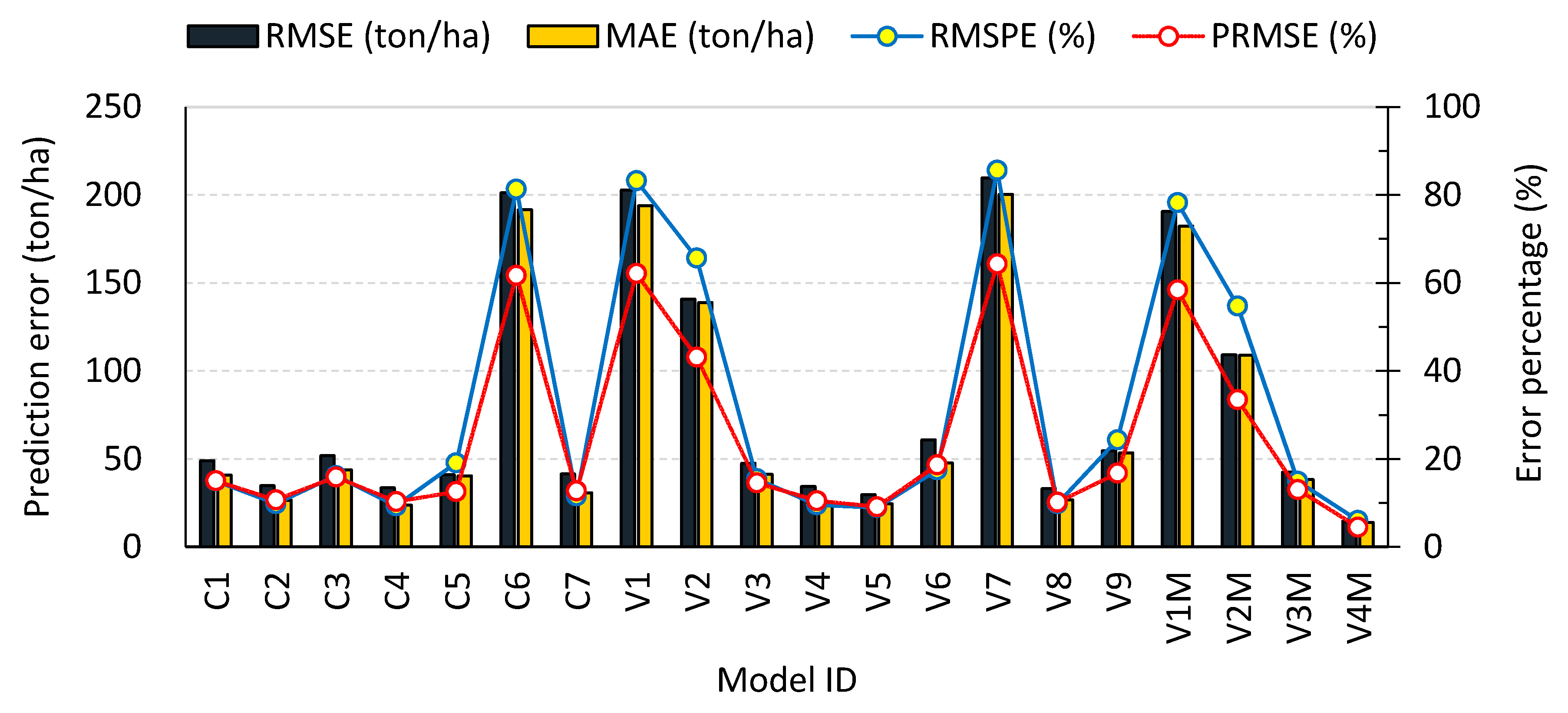
4.1. A Post-Hoc Examination of the Prediction Accuracy of AGC Stock Estimation at Stand-Level

As mentioned previously, various combinations of the LiDAR-derived tree metrics displayed mixed performance in estimating forest stand above-ground carbon. Of the 20 tree-level AGC models presented in this study, the least accurate was model V7 at the level of MAE = 200.27 ton/ha, RMSE = 209.74 ton/ha, PRMSE = 64.29%, and RMSPE = 85.59%. Assuming these values as the base values for prediction accuracy achievable via LiDAR-based AGC models, model V4M (MAE = 14.0 ton/ha, RMSE = 14.7 ton/ha, PRMSE = 6.0%, and RMSPE = 4.5%) showed an improvement of 92.99%, 93.01%, 93.01%, and 92.96%, respectively.

Table 6. Mean difference of the post hoc test for the average mean of AIP (%) of the AGC models.

Model ID	V4M	V5	C2	V4	V8	C4	C7	V3M	C5	V3
Mean (AIP)	93	87	86	86	86	86	83	81	80	79
Grouping	A	B	B, C	B, C	B, C	B, C	C, D	D, E	D, E	D, E
Model ID	C1	C3	V6	V9	V2M	V2	V1M	C6	V1	V7
Mean (AIP)	79	77	74	73	44	30	9	4	3	0
Grouping #	D, E	E, F	F, G	G	H	I	J	K	K, L	L

#: Models with the same alphabetical code indicates that the mean was statistically insignificant at the probability alpha = 0.05 based on the post hoc test using Duncan’s new multiple range method.

displays the accuracy improvement percentage (AIP) post hoc test using Duncan’s new multiple range test [41,42]. Models with the same alphabetical code were statistically insignificant at a probability level of 0.05. Obviously, a model that appropriately integrated LiDAR-derived tree metrics could improve AGC prediction accuracy. For example, models V4M, V4, V5, V8, C2, and C4 had the ability to improve AIP by at least 85% when compared to the base-level model V7. Duncan’s test suggested that the improvement in accuracy achieved by those six models was superior to the others. Model V4M achieved the best improvement with an AIP of 93% (Duncan grouping = “A”) and models V5, C4, V4, V8, and C2 were grouped as “B” indicated their AIPs were statistically equal.

4.2. Detrimental Combinations of LiDAR-Derived Tree Parameters and Increased Uncertainty in the Estimation of Stand-Level AGC

Figure 4 shows the variations between estimates of stand-level AGC stocks made as a result of ground-based inventory observations compared with estimates made by the 20 tree-level models. The tree-level models used various combinations of LiDAR-derived tree metrics. All the tree-level models were validated at the tree-level using the same assessment data as the stand-level and changes in the prediction error could be attributed to uncertainty. In this study, the prediction uncertainty of a model was measured by the difference between the model adequacy (R²) and the overall prediction performance (OPP) (Table 5).

Among the seven biomass-based models, models C2 and C4 revealed consistent estimation results between the measures R² and OPP while model C6 obviously not. Although the uncertainty in models C1, C3, C5, and C7 showed a moderate consistency, the difference between these four models was that C7 achieved a high degree of model adequacy and prediction performance while C1 and C3 obtained a medium level. This is because model C6 used only the metric LH while the other models integrated additional information from the other tree metrics. In contrast to model C5 which use only the predictor LDBH, an additional metric of LH, LCR, and LCI was gradually added to model C4, C3, C2, and C1 to describe the AGC variations of individual trees. Though these models were with high level of R², however, a significant loss of OPP in models C1 and C3 was greater than model C5. This kind of estimation inconsistency was probably induced by a poor combination of the tree metrics in models C1 and C3.

Model C1 had a variation inflation factor (VIF) of 50.2 and 39.4 for LDBH and LH and 3.6 and 4.2 for LCI and LCR. Similarly, LDBH, LH, and LCR in model C3 also has VIFs of 14.8, 12.8, and 2.3. The situations in C1 and C3 indicated a certain problem of multicollinearity which might lead to an inaccurate estimate(s) of the regression coefficients. Since the regression coefficient of LCR in models C1 and C3 was negative, which is counter to the positive linear relationship between LCR and AGC, the estimation performance should be a result of the interaction of the LDBH, LH, and LCR caused by their significant near-linear correlation in the inappropriate models. In contrast, models C2 and C4 should be free of multicollinearity because the VIFs of the models’ predictors were moderately small and each of their regression coefficients showed an identical positive sign to the relationship of the metrics. In addition, model C7 excluded LDBH and used the metrics LH, LCI, and LCR to achieve 88% of overall prediction accuracy with a VIF of 1.0–1.2 for each predictor. Comparing the difference of estimation performance between model C6 and models C2, C4, and C7 (Table 5), it could be concluded that LCI offered additionally critical information for estimating tree individuals’ AGC and therefore able to obtain appropriate accuracy for stand-level AGC estimation.

Among the volume-based group of models, a significant uncertainty of stand-level AGC estimation was found to the models V7 and V1M. Model V7 applied only a metric lnLH while model V1M applied Type-1 LDBH and LH in the form of Schumacher-Hall formula. These two models were able to account for the variation of tree individuals’ AGC stocks in the training dataset at a level of 84%, but offered an overall prediction performance of 25%–32% to the assessment dataset. The low performance of V7 was due to the shortage of volumetric information offered by using only one metric LH as the predictor. This situation was identical to model C6. Similarly, the low performance of V1M was contributed by the Type-1 LDBH because the secondary tree metric was a derivative of LH, that is LDBH1 = exp(1.479 + 0.864lnLH). The relationship of AGC and LH went overboard by models V1 and V1M. Models V2 and V2M copied some sort of the impacts caused by the over effects of LH and LCR, this is evident due to the Type-2 diameter metric was determined as LDBH2 = exp(1.473 + 0.835lnLH + 0.003LCR²). The overall estimation performance of the models V7, V1, V1M, V2, and V2M indicated that using only LH and LCR metrics in volume-based model was not able to achieve a reliable estimation of stand-level AGC stocks.

Apparently, when the metrics LCI and LCR were banded together with LH to create the volume-based tree-level model, model V5 achieved the most consistent results at an R² = 0.91 and a prediction accuracy of 91% (1-RMSPE ≈ 1-PRMSE). These two quantities revealed that the model V5 was almost capable of completely maintaining the same estimation performance in the validation dataset. As the LCR was replaced by its quadratic form, it did not detrimental to the performance of model V8 because the predictors’ coefficient in explaining the variations of tree-level AGC was appropriately tuned simultaneously. Similarly, the tree metrics of height, crown radius, and competition index can be effectively integrated in the Type-4 diameter metric to create model V4M. This type of Schumacher-Hall formula was exactly able to make an estimation performance almost identical to and even better than models V5 and V8 because model V4M got extra gain of prediction accuracy for OPP = 95% greater than R-squared = 91%. However, when crown radius was removed from the derivation of Type-3 diameter metric, a prediction uncertainty was introduced to the derived model V3M and caused a value of 4% performance reduction. This is evident in the line chart of error percentage as shown in Figure 4. On average, the models’ accuracy improvement percentage (shown in Table 5) of V4M was significantly greater than model V4 and model V3M by 7% and 12% respectively. Thus, by combining LH, LCI, and LCR in an appropriate method, a volume-based tree-level AGC model can be a reliable method to obtain acceptable accuracy at stand-level AGC prediction as well as the biomass-based AGC model.

Finally, the performance of the biomass-based and volume-based models shown in Table 1 and Table 2 varied widely. In fact, these two types of AGC models are very similar because they both apply the IPCC method of using factors, e.g., carbon fraction, wood density, and biomass expansion factor to derive above-ground carbon of trees, and use LiDAR-derived metrics with regression to get to different dependent variables, namely AGC and Volume. The key difference is that the factors are gained a priori in the biomass approach but a posterior in the volume approach. It appeared that given the factors involved and the errors with their estimation, the lower R² and/or estimation performance for some of the AGC models was due to uncertainty caused by multicollinearity for example C1 vs. C2, and due to unexplained variances introduced by using factors obtained from the literature, for example C7 vs. V5.

4.3. Why Use Biomass-Based or Volume-Based AGC Models in Predicting Forest Carbon Stock?

As discussed in previous sections, the value of each LiDAR-derived variable in predicting carbon stock was explored. Appropriate biomass-based and volume-based models are capable of making reliable AGC estimates. In brief, three tree-level AGC models were recommended to account for the forest carbon stocks based on their superior performance in both training and validation datasets:

(1)

biomass-based model C2: AGC = 0.000068159 × LDBH^1.4299 × LH^1.1708 × LCI^−0.0573,

(2)

volume-based model V4M: AGC = [0.2919(a × LDBHb × LHc)1.0026], and

(3)

volume-based model V5: AGC = [exp(−6.2803 + 2.3774lnLH − 0.0145LCI + 0.0316LCR)] × D × BEF × CF.

The LDBH in models C2 and V4M was determined using Equation (10). The forest ecosystem is known as the largest carbon sink in the terrestrial ecosystem but it could become the largest source of carbon emissions if deforestation and forest degradation occurs continuously. From the viewpoint of national/regional/global monitoring and assessment of forest ecosystem, to regularly gathering accurate forest carbon stocks in consistent and stable ways should be quite important for local forest management organizations and global forest resources evaluation agencies. As such, using biomass-based or volume-based AGC models for continuous forest inventory (CFI) over the terrestrial ecosystem is our major concern.

In practice, species-specific wood density, biomass expansion factor, and carbon fraction must be a priori determined in the biomass approach. This prerequisite of gathering those factors would not be a problem for plantations or small-scale forest stands. However, this approach might become a limitation for large-scale national inventory, especially in a forest ecosystem with complicated species compositions over a wide range of ecological amplitudes. In contrast, the volume approach would be more convenient for three reasons. Firstly, no such a priori factor determination is required before AGC modeling can be performed. Secondly, this technique can be implemented by directly linking the LiDAR metrics to tree volume and then posteriorly, above-ground carbon. Lastly, this method can achieve a reliable accuracy and offer an approach to assess national/regional/global forest carbon stocks in an IPCC-compatible method.

4.4. Recommendations for Future Work

As Bombelli et al. [22] suggested, regular in situ calculation of biomass/carbon stock via detailed forest inventory should not be postponed longer than five years. This is due to rapid changes in forest resources in some countries. High density airborne LiDAR data may be too costly for many undeveloped and developing countries to consider feasible. Further work that can effectively integrate tree-level AGC models and more stand-level metrics such as canopy cover may provide a cost-effective solution. In order to derive meaningful harmonized stand-level metrics of forest stand for such a purpose, Tomppo et al. [43] suggested a sample plot of 0.5 hectares would be appropriate. As a result, a terrestrial LiDAR technique [13,43,44,45,46,47] would be appropriate for collecting accurate ground data that minimize measurement uncertainty for stand-level AGC modeling. Additionally, it may be possible to use low resolution airborne LiDAR data or high-resolution satellite SAR images such as POLSAR [48] and TanDEM-X [49] to obtain parameters of forest canopy as the predictors of stand-level AGC models. This could reduce the cost of determining AGC forest stocks in the national/regional/global terrestrial ecosystems significantly.

The tree-level AGC modeling technique was developed based on airborne LiDAR-based CHM data. In general, a natural forest is generally composed of multiple canopy layers. This is particularly a common composition for broad-leaved forest. As a result, the trees grow beneath overstorey canopy will not be seen from the top and therefore could not be detected using the CHM data. In such case, high density full waveform airborne LiDAR data may help to detect tree crowns along the vertical canopy profile and the derived features would be suitable for developing a modified tree-level AGC modeling technique.

5. Conclusions

The amount of above-ground carbon storage in individual trees in a forest stand varies considerably due to variations in tree size, which occurs naturally in space and time. Regular assessment of forest resources on a national, regional, and global scale is particularly important in tackling carbon emissions due to deforestation and degradation. Airborne LiDAR data facilitates the construction of a three-dimensional forest model at sufficiently high spatial resolution to capture specific metrics. Tree size parameters can be derived from the metrics and used to assess above-ground carbon storage of individual trees and forest stands. This paper developed a range of tree-level AGC estimation models using the ground measurements of above-ground carbon and tree volume and LiDAR-derived diameter, height, crown radius, and competition index. Tree volume and AGC are positively related to tree diameter, height, and crown width as well as the tree metrics LDBH, LH, and LCR, while all the previous volumetric parameters are negatively related to the tree metric LCI. This relationship appears reasonable.

According the model validation procedure using the following accuracy indices: mean absolute error, root mean square error, percentage root mean square error and root mean square percentage error, it can be concluded that stand-level AGC stock can be accurately estimated using multiple combinations of the LiDAR-derived tree-level parameters. Specifically, a biomass-based tree-level AGC model employing the parameters LDBH, LH, and LCI in a power function performed very well. Estimates could account for 90% of the inventory-measured AGC stock in a forest stand. This performance was equal to a volume-based tree-level AGC model that used lnLH, LCI, and LCR as the predictors in an exponential formula. Performance of selected tree-level AGC models in the estimation of stand-level AGC stock was almost identical to the coefficient of determination of the model observed in tree-level AGC modeling. The parameters LH or lnLH, LCR, and LDBH tended to increase accuracy while LCI had a negative effect. Tree-level AGC models with LH, LCR, and LDBH, but without the LCI, had poor performance at the stand-level. We therefore conclude that LCI when banded together with LH and LCR or LDBH and LCR significantly improves the AGC estimation rate at the tree-level as well as the stand-level. It follows that the algorithm proposed in this study is appropriate for practical use in accounting for stand-level AGC stocks.

From the viewpoint of the FAO (Food and Agriculture Organization of the United Nations) who regularly make assessments of biomass and carbon stock changes in forests through the Global Forest Resources Assessment (FRA) [35], both biomass-based and volume-based tree-level AGC models make reliable estimates. The biomass-based approach needs a priori determination of carbon conversion factors, and some inconsistencies may arise when comparing results of national AGC inventories due to these factors. In contrast, the volume-based method can be easily implemented to estimate the above-ground carbon storage based on the IPCC defined protocol which is the accepted method for assessing the world’s forest resources [50]. In cases where species-specific biomass and carbon factors are not available, the volume-based method is suitable because the proxy coefficients of biomass and carbon conversion factors suggested by IPCC [51] can be applied directly. Since the IPCC also suggested the ratio of below-ground biomass to above-ground biomass as a constant [51], it is more convenient to extrapolate tree-level AGC to total carbon stock in forest stands. With multi-temporal LiDAR data, this technique can offer geospatially explicit information concerning forest productivity and has benefits in identifying forest ecosystem regions suitable for agricultural use or sustainable forest management [52].

References

1. Lin, C.; Lin, C.H. Comparison of carbon sequestration potential in agricultural and afforestation farming systems. Sci. Agricola 2013, 70, 93–101. [Google Scholar] [CrossRef]
2. Tsogt, K.; Lin, C. A flexible modeling of irregular diameter structure for the volume estimation of forest stands. J. For. Res. 2014, 19, 1–11. [Google Scholar] [CrossRef]
3. Popescu, S.C.; Wynne, R.H.; Scrivani, J.A. Fusion of small-footprint LiDAR and multispectral data to estimate plot-level volume and biomass in deciduous and pine forests in Virginia, USA. For. Sci. 2004, 50, 551–565. [Google Scholar]
4. Almeida, A.C.; Barros, P.L.C.; Monteiro, J.H.A.; Rocha, B.R.P. Estimation of above-ground forest biomass in Amazonia with neural networks and remote sensing. IEEE Lat. Am. Trans. 2009, 7, 27–32. [Google Scholar] [CrossRef]
5. Zhao, K.; Popescu, S.; Nelson, R. LiDAR remote sensing of forest biomass: A scale-invariant estimation approach using airborne lasers. Remote Sens. Environ. 2009, 113, 182–196. [Google Scholar] [CrossRef]
6. Badreldin, N.; Sanchez-Azofeifa, A. Estimating forest biomass dynamics by integrating multi-temporal Landsat satellite images with ground and airborne LiDAR data in the Coal Valley Mine, Alberta, Canada. Remote Sens. 2015, 7, 2832–2849. [Google Scholar] [CrossRef]
7. Hansen, E.H.; Gobakken, T.; Bollandsås, O.M.; Zahabu, E.; Næsset, E. Modeling aboveground biomass in dense tropical submontane rainforest using airborne laser scanner data. Remote Sens. 2015, 7, 788–807. [Google Scholar] [CrossRef] [Green Version]
8. Sheridan, R.D.; Popescu, S.C.; Gatziolis, D.; Morgan, C.L.S.; Ku, N.W. Modeling forest aboveground biomass and volume using airborne LiDAR metrics and forest inventory and analysis data in the Pacific Northwest. Remote Sens. 2015, 7, 229–255. [Google Scholar] [CrossRef]
9. Meyer, V.; Saatchi, S.S.; Chave, J.; Dalling, J.W.; Bohlman, S.; Fricker, G.A.; Robinson, C.; Neumann, M.; Hubbell, S. Detecting tropical forest biomass dynamics from repeated airborne LiDAR measurements. Biogeosciences 2013, 10, 5421–5438. [Google Scholar] [CrossRef]
10. Simonson, W.; Ruiz-Benito, P.; Valladares, F.; Coomes, D. Modelling above-ground carbon dynamics using multi-temporal airborne LiDAR: Insights from a Mediterranean woodland. Biogeosciences 2016, 13, 961–973. [Google Scholar] [CrossRef]
11. Jubanski, J.; Ballhorn, U.; Kronseder, K.; Franke, J.; Siegert, F. Detection of large above-ground biomass variability in lowland forest ecosystems by airborne LiDAR. Biogeosciences 2013, 10, 3917–3930. [Google Scholar] [CrossRef]
12. Lefsky, M.A. A global forest canopy height map from the Moderate Resolution Imaging Spectroradiometer and the Geoscience Laser Altimeter System. Geophys. Res. Lett. 2010, 37, L15401. [Google Scholar] [CrossRef]
13. Popescu, S.C.; Zhao, K.; Neuenschwander, A.; Lin, C. Satellite LiDAR vs. small footprint airborne LiDAR: Comparing the accuracy of aboveground biomass estimates and forest structure metrics at footprint level. Remote Sens. Environ. 2011, 115, 2786–2797. [Google Scholar] [CrossRef]
14. Los, S.O.; Rosette, J.A.B.; Kljun, N.; North, P.R.J.; Chasmer, L.; Suarez, J.C.; Hopkinson, C.; Hill, R.A.; van Gorsel, E.; Mahoney, C.; et al. Vegetation height and cover fraction between 60°S and 60°N from ICESat GLAS data. Geosci. Model Dev. 2012, 5, 413–432. [Google Scholar] [CrossRef]
15. Baccini, A.; Goetz, S.J.; Walker, W.S.; Laporte, N.T.; Sun, M.; Sulla-Menashe, D.; Hackler, J.; Beck, P.S.A.; Dubayah, R.; Friedl, M.A.; et al. Estimated carbon dioxide emissions from tropical deforestation improved by carbon density maps. Nat. Clim. Chang. 2012, 2, 182–185. [Google Scholar] [CrossRef]
16. Saatchi, S.S.; Harris, N.L.; Brown, S.; Lefsky, M.; Mitchard, E.T.A.; Salas, W.; Zutta, B.R.; Buermann, W.; Lewis, S.L.; Hagen, S.; et al. Benchmark map of forest carbon stocks in tropical regions across three continents. Proc. Natl. Acad. Sci. USA 2011, 108, 9899–9904. [Google Scholar] [CrossRef] [PubMed]
17. Gaveau, L.A.; Hill, R.A. Quantifying canopy height underestimation by laser pulse penetration in small-footprint airborne laser scanning data. Can. J. Remote Sens. 2003, 29, 650–657. [Google Scholar] [CrossRef]
18. Magnussen, S.; Nasset, E.; Gobakken, T. Reliability of LiDAR derived predictors of forest inventory attributes: A case study with Norway spruce. Remote Sens. Environ. 2010, 114, 700–712. [Google Scholar] [CrossRef]
19. Niska, H.; Skon, J.P.; Packalen, P.; Tokola, T.; Maltamo, M.; Kolehmainen, M. Neural networks for the prediction of species-specific plot volumes using airborne laser scanning and aerial photographs. IEEE Trans. Geosci. Remote Sens. 2010, 48, 1076–1085. [Google Scholar] [CrossRef]
20. Tesfamichael, S.G.; van Aardt, J.A.N.; Ahmed, F. Estimating plot-level tree height and volume of Eucalyptus grandis plantations using small-footprint, discrete return LiDAR data. Progress Phys. Geogr. 2010, 34, 515–540. [Google Scholar] [CrossRef]
21. Clark, D.B.; Clark, D.A. Landscape-scale variation in forest structure and biomass in a tropical rain forest. For. Ecol. Manag. 2000, 137, 185–198. [Google Scholar] [CrossRef]
22. Bombelli, A.; Avitabile, V.; Balzter, H.; Marchesini, L.B.; Bernoux, M.; Brady, M.; Hall, R.; Hansen, M.; Henry, M.; Herold, M.; et al. Biomass—Assessment of the Status of the Development of the Standards for the Terrestrial Essential Climate Variables; Global Terrestrial Observing System, Food and Agricultural Organization of United Nations: Rome, Italy, 2009. [Google Scholar]
23. Tsui, O.W.; Coops, N.C.; Wulder, M.A.; Marshall, P.L.; McCardle, A. Using multi-frequency radar and discrete-return LiDAR measurements to estimate above-ground biomass and biomass components in a coastal temperate forest. ISPRS J. Photogramm. Remote Sens. 2012, 69, 121–133. [Google Scholar] [CrossRef]
24. Maselli, F.; Chiesi, M.; Montaghi, A.; Pranzini, E. Use of ETM+ images to extend stem volume estimates obtained from LiDAR data. ISPRS J. Photogramm. Remote Sens. 2011, 66, 662–671. [Google Scholar] [CrossRef]
25. Zhao, F.; Guo, Q.; Kellya, M. Allometric equation choice impacts LiDAR-based forest biomass estimates: A case study from the Sierra National Forest, CA. Agric. For. Meteorol. 2012, 165, 64–72. [Google Scholar] [CrossRef]
26. Jakubowski, M.K.; Li, W.; Guo, Q.; Kelly, M. Delineating individual trees from LiDAR data: A comparison of vector- and raster-based segmentation approaches. Remote Sens. 2013, 5, 4163–4186. [Google Scholar] [CrossRef]
27. Popescu, S.C. Estimating biomass of individual pine trees using airborne LiDAR. Biomass Bioenergy 2007, 31, 646–655. [Google Scholar] [CrossRef]
28. Chen, Q.; Gong, P.; Baldocchi, D.; Tian, Y.Q. Estimating basal area and stem volume for individual trees from LiDAR data. Photogramm. Eng. Remote Sens. 2007, 73, 1355–1365. [Google Scholar] [CrossRef]
29. Dean, T.J.; Cao, Q.V.; Roberts, S.D.; Evans, D.L. Measuring heights to crown base and crown median with LiDAR in a mature, even-aged loblolly pine stand. For. Ecol. Manag. 2009, 257, 126–133. [Google Scholar] [CrossRef]
30. Dalponte, M.; Bruzzone, L.; Gianelle, D. A system for the estimation of single-tree stem diameter and volume using multireturn LiDAR data. IEEE Trans. Geosci. Remote Sens. 2011, 49, 2479–2490. [Google Scholar] [CrossRef]
31. Dalponte, M.; Coops, N.C.; Bruzzone, L.; Gianelle, D. Aanlysis on the use of multiple returns LiDAR data for the estimation of tree stems volume. IEEE J. Sel. Top. Appl. Earth Obs. Remote Sens. 2009, 2, 310–318. [Google Scholar] [CrossRef]
32. Barilotti, A.; Sepic, F. Assessment of forestry parameters at single-tree level by using methods of LiDAR data analysis and processing. Ambiência 2010, 6, 81–92. [Google Scholar]
33. Lin, C.; Lo, C.S.; Thomson, G. Estimating individual tree characteristics using the MMAC algorithm and a LiDAR -derived canopy height model. J. Earth Sci. Eng. 2011, 1, 35–41. [Google Scholar]
34. Lo, C.S.; Lin, C. Growth-competition-based stem diameter and volume modeling for tree-level forest inventory using airborne LiDAR Data. IEEE Trans. Geosci. Remote Sens. 2013, 51, 2216–2226. [Google Scholar] [CrossRef]
35. Forest Resources Assessment FAO. Global Forest Resources Assessment 2015—How Are the World’s Forests Changing; Food and Agricultural Organization of United Nations: Rome, Italy, 2015. [Google Scholar]
36. IPCC. Good Practice Guidance for Land Use, Land-Use Change and Forestry; IPCC/OECD/IEA/IGES: Hayama, Japan, 2003. [Google Scholar]
37. Lin, C.; Thomson, G.; Lo, C.S.; Yang, M.S. A multi-level morphological active contour algorithm for delineating tree crowns in mountainous forest. Photogramm. Eng. Remote Sens. 2011, 77, 241–249. [Google Scholar] [CrossRef]
38. Wang, C.H.; Feng, F.L.; Lin, C.; Wang, Y.C.; Wang, Y.N.; Lin, S.T.; Chiou, C.R.; Yen, C.H.; Chung, Y.L.; Liu, C.P.; et al. Constructing Models for Transforming Forest Stock into Biomass (1/3); Technical Report No. 95AS-12.3.5-e2; Taiwan Forestry Bureau: Taipei, Taiwan, 2006.
39. Hyndman, R.; Koehler, A. Another look at measures of forecast accuracy. Int. J. For. 2006, 22, 679–688. [Google Scholar] [CrossRef]
40. Lin, C.; Dugarsuren, N. Deriving the spatiotemporal NPP pattern in terrestrial ecosystems of Mongolia using MODIS imagery. Photogramm. Eng. Remote Sens. 2015, 81, 587–598. [Google Scholar] [CrossRef]
41. Duncan, D.B. Multiple range and multiple F tests. Biometrics 1955, 11, 1–42. [Google Scholar] [CrossRef]
42. Montgomery, D.C. Design and Analysis of Experiments, 2nd ed.; John Wiley & Sons: Hoboken, NJ, USA, 1984; pp. 66–68. [Google Scholar]
43. Tomppo, E.; Gschwantner, T.; Lawrence, M.; McRoberts, R.E. National Forest Inventories—Pathways for Common Reporting; Springer: Dordrecht, The Netherlands, 2010. [Google Scholar]
44. Santoro, M.; Eriksson, L.; Fransson, J. Reviewing ALOS PALSAR backscatter observations for stem volume retrieval in Swedish forest. Remote Sens. 2015, 7, 4290–4317. [Google Scholar] [CrossRef]
45. Liang, X.; Kankare, V.; Hyyppä, J.; Wang, Y.; Kukko, A.; Haggrén, H.; Yu, X.; Kaartinen, H.; Jaakkola, A.; Guan, F.; et al. Terrestrial laser scanning in forest inventories. ISPRS J. Photogramm. Remote Sens. 2016, 115, 63–77. [Google Scholar] [CrossRef]
46. Hosoi, F.; Nakai, Y.; Omasa, K. 3-D voxel-based solid modeling of a broad-leaved tree for accurate volume estimation using portable scanning LiDAR. ISPRS J. Photogramm. Remote Sens. 2013, 82, 41–48. [Google Scholar] [CrossRef]
47. Kankare, V.; Holopainen, M.; Vastaranta, M.; Puttonen, E.; Yu, X.; Hyyppä, J.; Vaaja, M.; Hyyppä, H.; Alho, P. Individual tree biomass estimation using terrestrial laser scanning. ISPRS J. Photogramm. Remote Sens. 2013, 75, 64–75. [Google Scholar] [CrossRef]
48. Abdullahi, S.; Kugler, F.; Pretzsch, H. Prediction of stem volume in complex temperate forest stands using TanDEM-X SAR data. Remote Sens. Environ. 2016, 174, 197–211. [Google Scholar] [CrossRef]
49. Zolkos, S.G.; Goetz, S.J.; Dubayah, R. A meta-analysis of terrestrial aboveground biomass estimation using LiDAR remote sensing. Remote Sens. Environ. 2013, 281, 289–298. [Google Scholar] [CrossRef]
50. Marklund, L.G.; Schoene, D. Global assessment of growing stock, biomass and carbon stock. In Forest Resources Assessment Programme Working Paper 106/E; FAO: Rome, Italy, 2006; p. 55. [Google Scholar]
51. IPCC. Guidelines for National Greenhouse Gas Inventories—Volume 4: Agriculture, Land Use and Forestry (GL-AFOLU). Available online: http://www.ipcc-nggip.iges.or.jp/public/2006gl/vol4.html (accessed on 10 December 2014).
52. Lin, C.; Trianingsih, D. Identifying forest ecosystem regions for agricultural use and conservation. Sci. Agricola 2016, 73, 62–70. [Google Scholar] [CrossRef]
Figure 1. Illustration of the study site location (a) and its ortho-rectified bitmap image (b) and canopy height model (c).
Remotesensing 08 00528 g001
Figure 2. Flowchart of the above-ground-biomass carbon accounting process.
Remotesensing 08 00528 g002
Figure 3. The relationship between a subject tree and its competitors. (a) The proximity area is defined based on the location of the subject tree and a radius r; (b) The angle θ i j is the competition pressure exerted on a subject tree i by a neighboring tree j in the proximity area.
Remotesensing 08 00528 g003
Figure 4. Prediction error variations of the tree-level AGC models in predicting stand-level AGC stocks.
Remotesensing 08 00528 g004