Article

Synergistic Use of Citizen Science and Remote Sensing for Continental-Scale Measurements of Forest Tree Phenology

Appalachian Laboratory, University of Maryland Center for Environmental Science, Frostburg, MD 21532, USA
*
Author to whom correspondence should be addressed.
Remote Sens. 2016, 8(6), 502; https://doi.org/10.3390/rs8060502
Submission received: 30 December 2015 / Revised: 17 May 2016 / Accepted: 31 May 2016 / Published: 14 June 2016
(This article belongs to the Special Issue Citizen Science and Earth Observation)

Abstract

:
There is great potential value in linking geographically dispersed multitemporal observations collected by lay volunteers (or “citizen scientists”) with remotely-sensed observations of plant phenology, which are recognized as useful indicators of climate change. However, challenges include a large mismatch in spatial scale and diverse sources of uncertainty in the two measurement types. These challenges must be overcome if the data from each source are to be compared and jointly used to understand spatial and temporal variation in phenology, or if remote observations are to be used to predict ground-based observations. We investigated the correlation between land surface phenology derived from Moderate Resolution Imaging Spectrometer (MODIS) data and citizen scientists’ phenology observations from the USA National Phenology Network (NPN). The volunteer observations spanned 2004 to 2013 and represented 25 plant species and nine phenophases. We developed quality control procedures that removed observations outside of an a priori determined acceptable period and observations that were made more than 10 days after a preceding observation. We found that these two quality control steps improved the correlation between ground- and remote-observations, but the largest improvement was achieved when the analysis was restricted to forested MODIS pixels. These results demonstrate a high degree of correlation between the phenology of individual trees (particularly dominant forest trees such as quaking aspen, white oak, and American beech) and the phenology of the surrounding forested landscape. These results provide helpful guidelines for the joint use of citizen scientists’ observations and remote sensing phenology in work aimed at understanding continental scale variation and temporal trends.

Graphical Abstract

1. Introduction

The phenology of deciduous trees and shrubs is sensitive to inter-annual variation in climate and therefore is considered a useful indicator of the impact of climatic change on forest processes [1]. Scientific understanding of these impacts has benefited from long-term monitoring of forest phenology at a range of spatial scales [2,3,4]. Monitoring of individual organisms has enabled the development of successful models that can predict phenology from seasonal climatic conditions [5,6,7]. At regional to global extents, satellite remote sensing data have effectively been used to capture the land surface phenology over time [8]. However, land surface phenology at this scale is viewed as the cumulative response of many individual organisms within each remote sensing pixel in combination with other land surface changes (e.g., soil moisture changes) [9], and is therefore fundamentally different than field-based observations of individuals [10,11,12].
For some areas of inquiry, geographically distributed phenology observations of individual plants in natural ecological settings are required, and remote sensing is a reasonable avenue to pursue such data. One such area concerns the examination of intraspecific genotype-phenotype relationships across environmental gradients. Accurate phenotyping of plants in their environment remains a grand challenge, and currently limits the rapid advance of the genotype-phenotype mapping required to understand local adaptation of plants to environment and locale-specific plant responses to environmental stress [13,14,15]. Response to this need can only be made through techniques that annually simultaneously collect phenophase observations over broad geographic areas. Remote sensing is one such method, but despite decades of work studying phenology from both ends of the spatial-scale spectrum (e.g., [8,12,16]), there remains considerable skepticism that moderate resolution remote sensing phenology provides a useful context for understanding the phenology of individual plants [17]. To address this challenge, paired observations from ground-based observations and remotely sensed imagery must be acquired across these broad geographic areas, and across multiple growing seasons. However, collection of such extensive field-based observations is often unrealistic for traditional science research teams of a few scientists and students.
A potential solution to the problem of collecting geographically dispersed, multitemporal observations of phenology is to harnesses the power of many volunteer observers, or “citizen scientists”. The growing field of citizen science directly immerses lay people in the process of research to help advance science-based knowledge. Citizen scientists are well suited to contribute to landscape and ecosystem ecology studies because they can make observations across broad temporal and spatial scales [18,19,20]. When coupled with standardized protocols, thousands of volunteers could be recruited to accurately phenotype many individual plants in their environment over the course of decades [21]. Several large programs have been initiated internationally to support volunteers in plant phenology investigations and serve as data sources for many research projects; in the United States, these include Nature’s Notebook (NN) managed by the USA National Phenology Network and Project Budburst managed by the National Ecological Observation Network.
Citizen science efforts offer multiple benefits including contributing to research findings; enhancing volunteers’ science skills and knowledge; and addressing social-ecological outcomes such as enhanced habitat, established protected areas, and improved relationships between communities and management agencies [22]. Despite such benefits, this approach is often underutilized in part due to concerns about quality of data collected by volunteers such as under-detection and lack of precision in measurements [23,24]. For example, variation in observer accuracy has been measured between trained volunteers and professionals [25] and between younger and older student volunteers [26], as well as across gradients in the size of the organism being observed [27], and by phenophase and species [28]. However, other studies have demonstrated that with appropriate training and experience volunteers, even those with limited formal science education, can produce data similar to professional scientists (e.g., [29,30,31]). For example, NN volunteers correctly identified plant phenophase 91% of the time when compared with expert observations [28]. The efficacy of volunteers’ efforts is also apparent in the extensive and diverse scientific publications resulting from their labors [19], including those focused on plant phenology (e.g., [32,33]).
Despite the potential value of citizen science and remotely-sensed phenology observations to support research across environmental gradients, few studies have carefully examined challenges of linking these two very different yet extensive and spatially-explicit datasets. Here, we sought to understand and address these challenges by assessing the degree of correspondence between citizen science ground-based observations and remote-sensing observations provided by the Moderate Resolution Imaging Spectrometer (MODIS) vegetation dynamics product. We focused on volunteer data collected as part of the NN program. The work required the assembly of NN volunteer observations for a wide range of deciduous trees and shrubs, including establishment of best practices for removing anomalous observations. For a selection of two model species, we looked in detail at the comparison between NN and MODIS across all years and phenophases recorded and evaluated the impact of the data management steps. Our work will address the potential for synergistic use of MODIS phenology with citizen science observations for many purposes, including the rapid phenotyping of plants in their natural environment across space and time.

2. Materials and Methods

2.1. Assembling Citizen Science Observations of Phenology

The National Phenology Network (NPN) maintains and promotes NN as a national online tool for amateur naturalists and professionals to voluntarily record phenology observations. Each NN observation includes records of multiple phenophase states exhibited by a life form on Earth. For this work, we used the NN database to acquire all relevant woody plant phenophases collected before 1 January 2014. Because phenophase names used by NN have changed slightly over time, and to increase the number of observations in any given category, we combined related phenophases. The resulting phenophases used for this work were (1) breaking leaf buds; (2) open flowers; (3) full flowering; (4) end of flowering; (5) pollen; (6) fruits; (7) leaves; (8) colored leaves; and (9) fallen leaves. For each plant-phenophase combination volunteers are asked to record either ‘yes’ (the phenophase is apparent), ‘no’ (the phenophase is not apparent), or ‘I don’t know’. On average, volunteers observe ~3 plants at any one site, but this number can be higher. Volunteers are encouraged to make regular observations of their selected plant(s). Observations made before a phenophase has developed are recorded as ‘no’ in that a phenophase was not observed. Clearly, observers who visit an individual more frequently will not only make more ‘no’ records, but will also have a better chance to record an earlier date for the first occurance of any given phenophase (i.e., reduce the time between the last ‘no’ record and the first ‘yes’ record).
We extracted a list of observations from the NN database spanning a range of deciduous forest-dwelling species (https://www.usanpn.org/results/data). The resulting list of records was subsequently refined through a two-step process:
  • We sorted by the number of sites where each species was observed and selected all species that were observed at more than 30 sites.
  • We sorted by the number of individuals observed at each site, and selected all observations made at sites with five or more species observed.
This resulted in a list of observations representing 25 species (Table 1). These 25 species were deemed satisfactorily broad in distribution; yet, by constraining to sites with five or more species per site, we ensured that the distributions also overlapped, reducing the importance of geographic range on the degree of phenotypic variation within species. Most selected species were forest-dwelling trees that are often dominant in the stands they occupy. However, shorter, understory trees (e.g., Acer negundo, Cercis canadensis, Cornus florida) and shrubs (e.g., Forsythia × intermedia, Syringa vulgaris) were also represented, allowing the consideration of the importance of crown position and plant size on the relationship between volunteer ground observations and MODIS phenology.
The NPN considers two of the species in our selected data to be calibration species: quaking aspen (Populus tremuloidies) and Red Rothomagensis lilac (Syringa × chinensis) (NPN website). Calibration species have broad distributions and are ecologically or economically important. For these species, we included all observations (i.e., skipped steps 1 and 2 above for these species) and conducted extra analyses such as producing scatter plots. One advantage of using P. tremuloidies as a study species is that it occurs in clonal stands that are potentially large enough to be directly observed in moderate resolution imaging spectrometry. To these observations, we added observations of Populus balsamifera. While P. balsamifera is less common in the contiguous United States than is P. tremuloidies, it can also be found in dense clonal stands. Both Populus species have another distinct advantage for study in that their genomes have been sequenced, and studies relating continental variation in genotype to phenotype have been conducted. These studies have shown that populations from northern climates are locally adapted to require a lower (shorter) intrinsic heat requirement (i.e., growing degree days) to spur release from ecodormancy [14]. Syringa × chinensis (Red Rothomagensis lilac) was selected for study due to the long history of lilac in work on phenology [5], the large number of NN observations available, and its contrast to the Populus species in terms of growth form (tree vs. shrub) and flower size (S. × chinensis has a large showy flower that is easy for volunteers to observe). Observers may do better at accurately assessing phenophase status in a plant with showy flowers, as opposed to deciduous forest trees, where the flowers are quite smaller and possibly more distant from the observer.
Processing of the NN data began by searching the observation list for repeat observations of the same plant within each growing season. For each year, we identified the first ‘yes’ record for each phenophase (i.e., the phenophase onset), and recorded this date along with the date of the previous ‘no’ observation. We then created two quality control steps on the NN dataset to reduce the observations to a list that could be compared against annual MODIS observations:
Rule #1.
We removed outlier observations by setting a priori thresholds to the date range in which acceptable observations could be made. This step was motivated by the observation that some NN phenophases that could be characterized as “spring phenophases” (e.g., flowers) were recorded as occurring in autumn, and “autumn phenophases” (e.g., colored leaves) were recorded as occurring in spring. The date range for acceptable observations in spring varied by species and phenophase, but was never earlier than DOY 50 or later than DOY 200. For autumn phenophases we accepted observations between DOY 200 and DOY 365.
Rule #2.
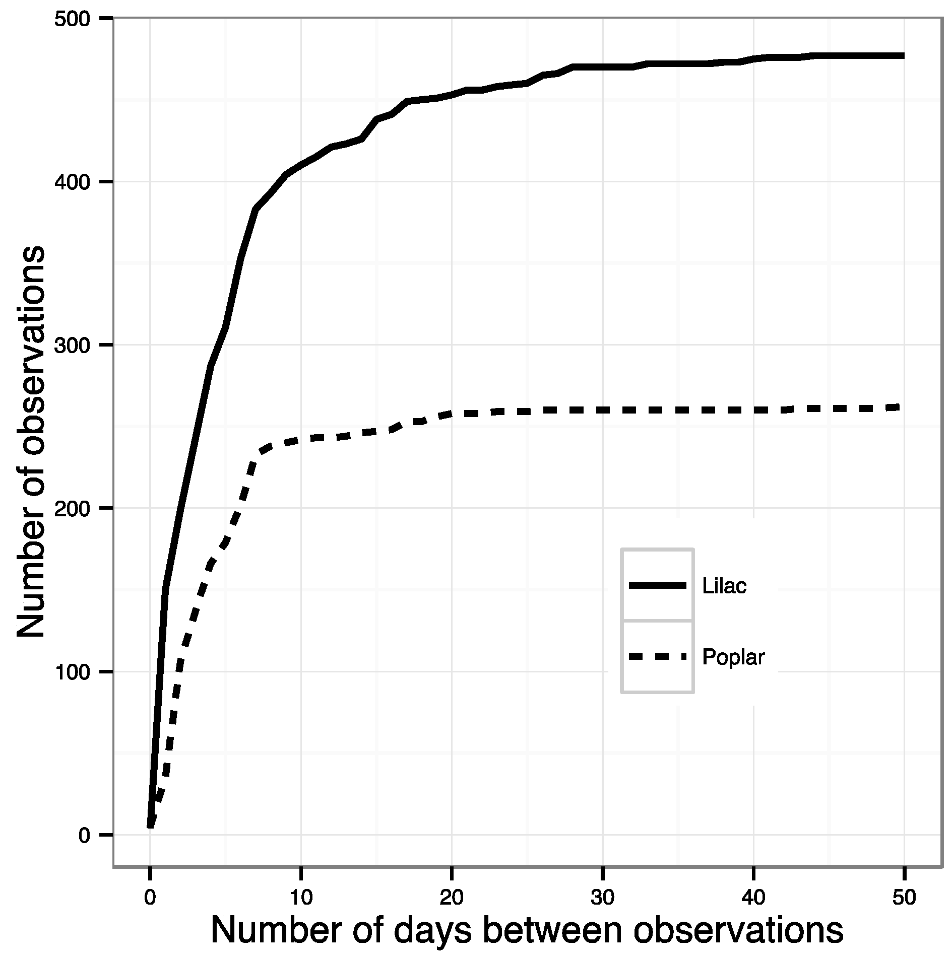
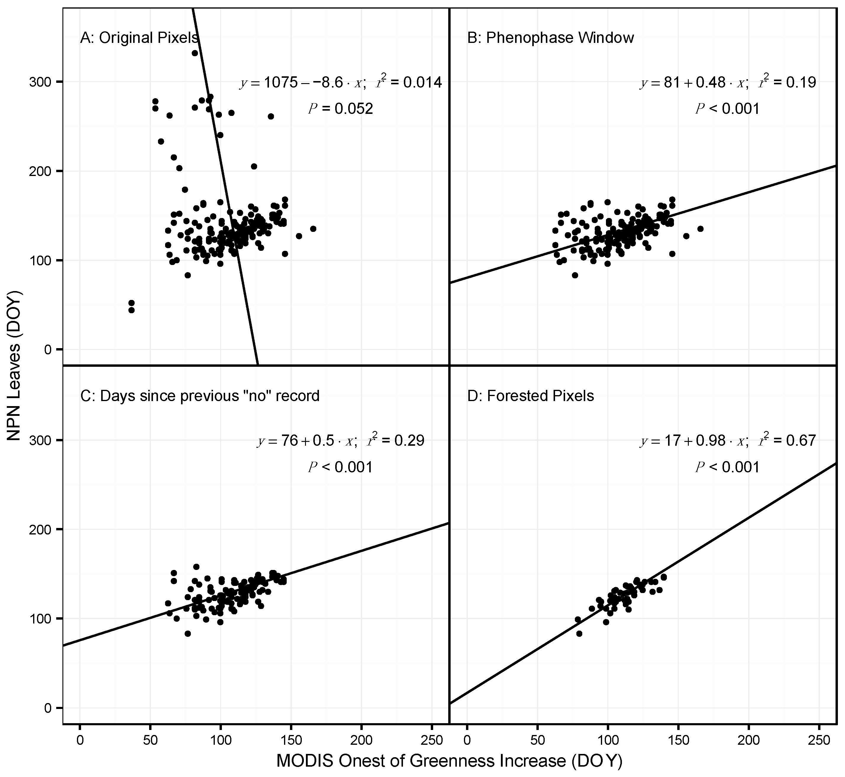
All phenophase onset records were removed that were not preceded by a ‘no’ observation within the previous ~10 days. This effectively removed all observations made by volunteers who were not regularly visiting their plants and did not submit records to NN that were frequent enough to ensure a timely observation of an emerging phenophase. The specific threshold was identified by calculating the number of observations remaining after successive shortening of this window. The best threshold balances the need to use as many observations as possible with the need for regular observations of the same plant (Figure 1). The threshold number of days was 10 for most species; however, for some species this was lengthened after examining the effect on sample size (Table S1).

2.2. MODIS Phenology Product and Post-Processing

The MODerate Resolution Imaging Spectrometer (MODIS) Vegetation Dynamics product (MCD12Q2), which is provided annually, was downloaded for all of North America. Data were mosaicked and reprojected (nearest neighbor resampling) to a Geographical Coordinate System and exported in a GEOTiff file format. For each year, four phenology dates are provided by MCD12Q2, these are the dates of Onset of Greenness Increase (OGI), Onset of Greenness Maximum (OGMax), Onset of Greenness Decrease (OGD), and the Onset of Greenness Minimum (OGMin) [34]. MCD12Q2 also includes a quality assurance/quality control (QAQC) layer indicating pixels for which a phenology estimate from the remote sensing time series was not calculated. This layer was used to remove all NN observations falling on “No Data” pixels in any given year.
The geographic location of each NN site was identified in the MODIS phenology data, defining a focal MODIS pixel for each NN record. An initial comparison of the NN and MODIS phenology records for the focal pixel revealed that non-forest land cover within some focal pixels resulted in highly variable phenology estimates that did not correlate well with NN observations (more detail in results). Therefore, we developed a third component of quality control that used the MODIS land cover product (MCD12Q1) to identify all forested pixels (classified as one of the following: Deciduous Needle leaf forest, Deciduous Broadleaf forest, and Mixed forest) occurring within the 9 pixels surrounding and including the focal MODIS pixel. If no forested pixel was identified, the site was dropped from the analysis. If between 1 and 9 forested pixels were identified, we calculated the median MODIS phenology date for each of the four MODIS phenophases. These median values were used in all subsequent analyses.

2.3. Statistical Analyses

Our overall strategy was to build linear regression models comparing NN phenophase onset dates with MODIS phenology dates. Because measurement uncertainty was assumed in both the effect (MODIS) and response (NN records) variables, we used type 2 regression (major axis regression). For each species, we considered models constructed between a wide range of NN phenophases and MODIS phenology markers, and used data across all available years. While some variable combinations might be considered unlikely to correlate (e.g., NN flowering phenophases with MODIS onset of greenness increase), we wanted to avoid making important decisions on which variables to include in the analysis based on pre-conceived notions of what would and what wouldn’t correlate. This inclusive approach also recognizes that there may be consistent offsets between NN phenophases that would strengthen relationships with MODIS despite no logical pathway through which MODIS could be directly observing the phenophase. Further, despite reference to greenness transitions in the names of each MODIS phenology marker, these markers are influenced by changes in land surface phenology (broadly speaking), which could increase or decrease the correlation between NN phenophases and MODIS. This being said, we decided not to compare phenophases consistently occurring in autumn (Colored leaves and Fallen leaves) with MODIS spring phenology dates.
Because the NN phenophases were not all recorded with the same temporal frequency, the number of observations in each regression model was highly variable. We limited the analysis to only those regressions that were significant at the p < 0.05 level. We further evaluated the influence of the number of observations on the NN-MODIS correlation. We found that the mean model correlation (across all significant regressions) was influenced by a small number of regressions formed from just 3–5 observations reporting very high model performance (e.g., R2 > 0.95). While these were significant regressions (p < 0.05), we were not interested in drawing conclusions from such a small sample size. Therefore, we decided to limit the analysis to those models where the number of observations ≥10.
After excluding NN-MODIS correlations with fewer than 10 observations, we compared the distribution of R2 values across different levels of organization. Box plots were generated to explore variation in NN-MODIS correlation by species, NN phenophase, MODIS phenophase, and canopy position (upper canopy vs. lower canopy trees). TukeyHSD was used to identify significant differences between regression statistics grouped by phenophase, species, and lifeform. Further analysis of the performance of the two calibration species (poplar and lilac) included inspection of scatter plots and additional analyses to determine the effect of key processing steps. Finally, for the two models of poplar leaves and lilac full flowering, we calculated prediction intervals, thus providing uncertainty estimates for using MODIS to predict NN volunteer observations. All analyses were completed in the R statistical programing language.

3. Results

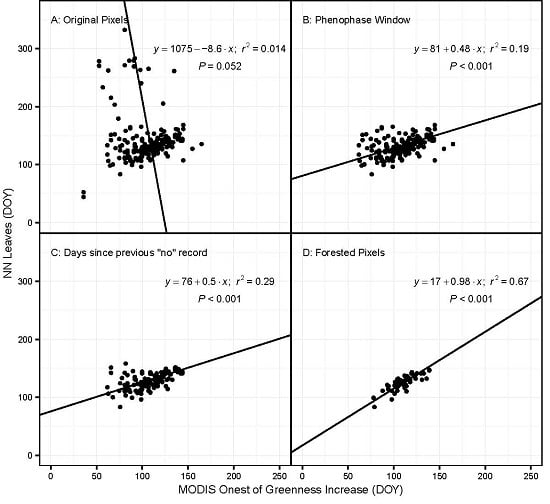
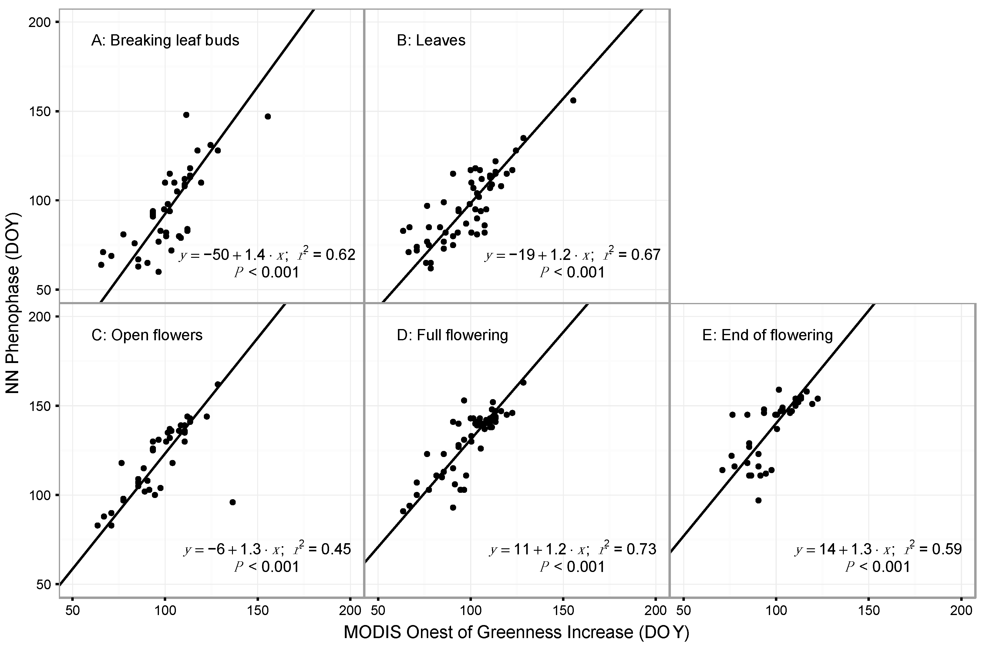
3.1. Model Performance for Poplar and Lilac

Regression models between MODIS and NN phenophases improved in response to each of quality control procedures. The case for NN observations of poplar leaves was characteristic of this improvement (Figure 2). Before any quality control on the NN observations (but including the removal of observations with no MODIS phenology due to clouds or other MODIS phenology algorithm failures), we found that the correlation between MODIS and NN observations was not significant (R2 = 0.014; p = 0.052). The removal of NN observations outside of the a priori identified phenophase temporal window (Rule #1) improved the correlation (R2 = 0.19; p < 0.001). Further improvement was achieved by restricting the data to records of ‘yes’ with a preceding ‘no’ record within an a priori determined period (Rule #2) (R2 = 0.29; p < 0.001). However, the largest incremental improvement in the model R2 was achieved by limiting the analysis to the median MODIS phenology of forested pixels adjacent to and including the pixel containing the NN observation (R2 = 0.67; p < 0.001). This large improvement was seen for lilac, as well with the final model of NN observations of lilac full flowering exceeding the correlation of poplar (R2 = 0.73; p < 0.001).
The quality control procedures employed removed 76% of the NN observations of poplar and lilac combined. Enforcing the a priori window of acceptable observations had the smallest impact on sample size, reducing the observations of poplar by 11% and lilac by 3%. Restricting the number of days between observations to less than an a priori determined threshold accounted for a 30% and 37% reduction for poplar and lilac, respectively. The largest effect on sample size was the removal of non-forested pixels. Here, 57% and 70% of remaining NN observations (i.e., remaining after the previous two quality control steps) were identified as located in non-forested areas and were removed from the analysis. The number of remaining poplar and lilac observations was 73 and 90, whittled down from original values of 272 and 495, an overall reduction of 73% and 82%, respectively.
These statistics for NN observations of poplar leaves and lilac full flowering paralleled statistics for the other phenophases of these species. Final model performance for poplar and lilac ranged from R2 = 0.32 (poplar Breaking leaf Buds; Figure 3) to R2 = 0.73 (lilac full flowering; Figure 4). Across these models, we also observed a large range in the number of observations, with NN observers of poplar trees more commonly making leaf-related phenophases than flower-related phenophases. The opposite was true for observations of lilac, but the difference was smaller. Despite differences in the slope and R2, calculated prediction intervals for poplar leaves and lilac full flowering were ±15 days. We made these calculations after making the NN observation the response variable and switching to least squares regression; therefore, ±15 days is the uncertainty of using a MODIS OGI observation to predict an NN volunteer observation within 750 m (1.5 MODIS pixels) of any MODIS pixel.

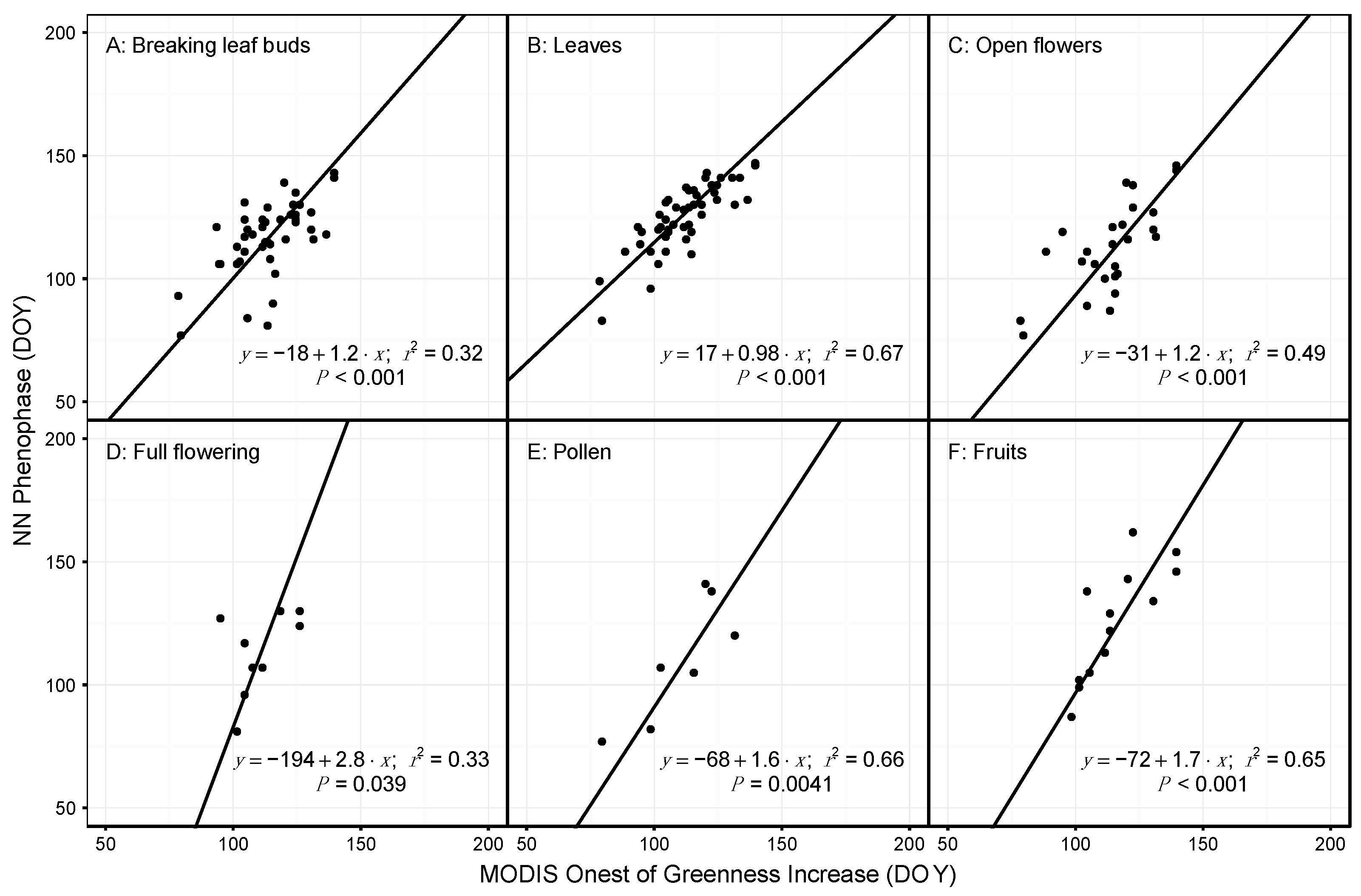
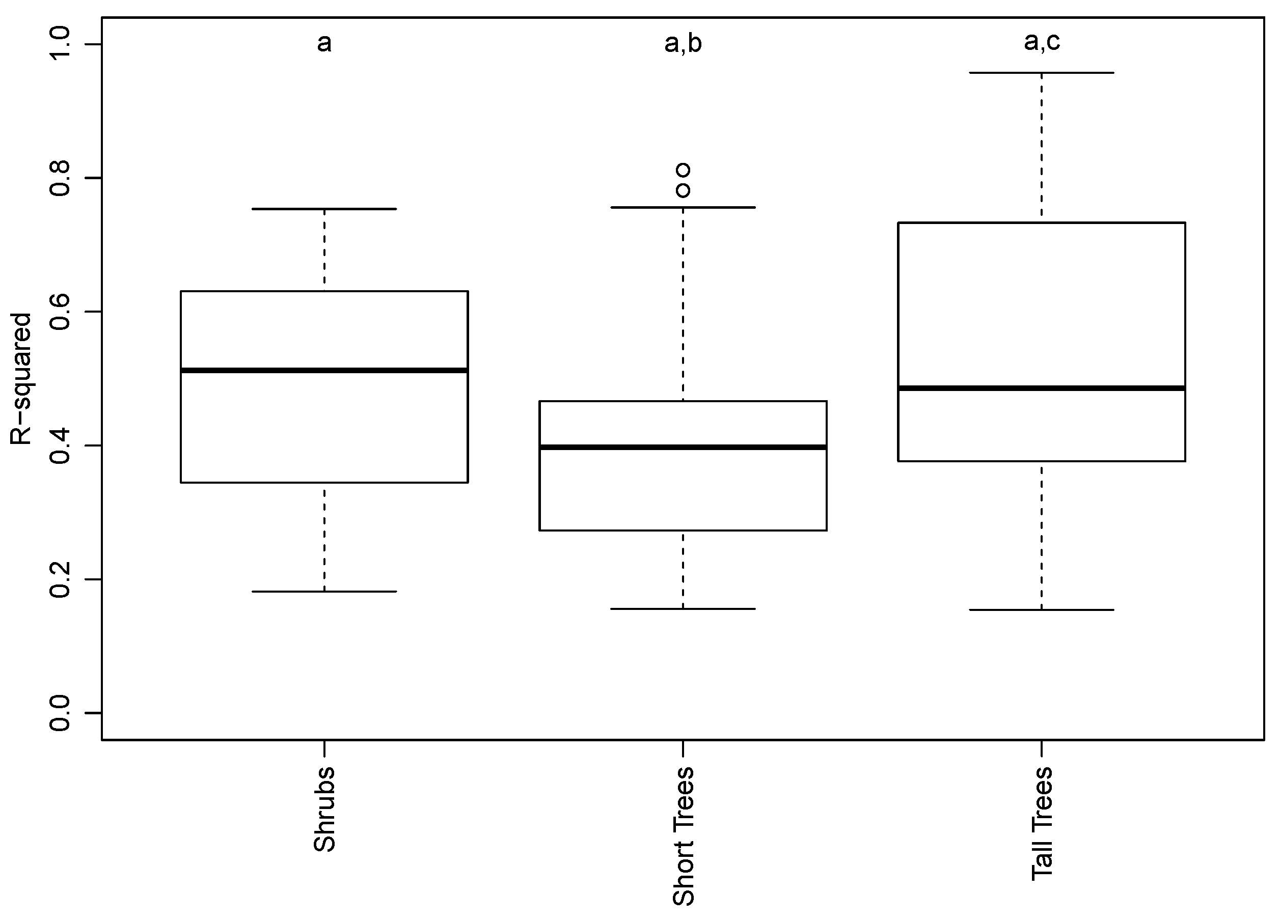
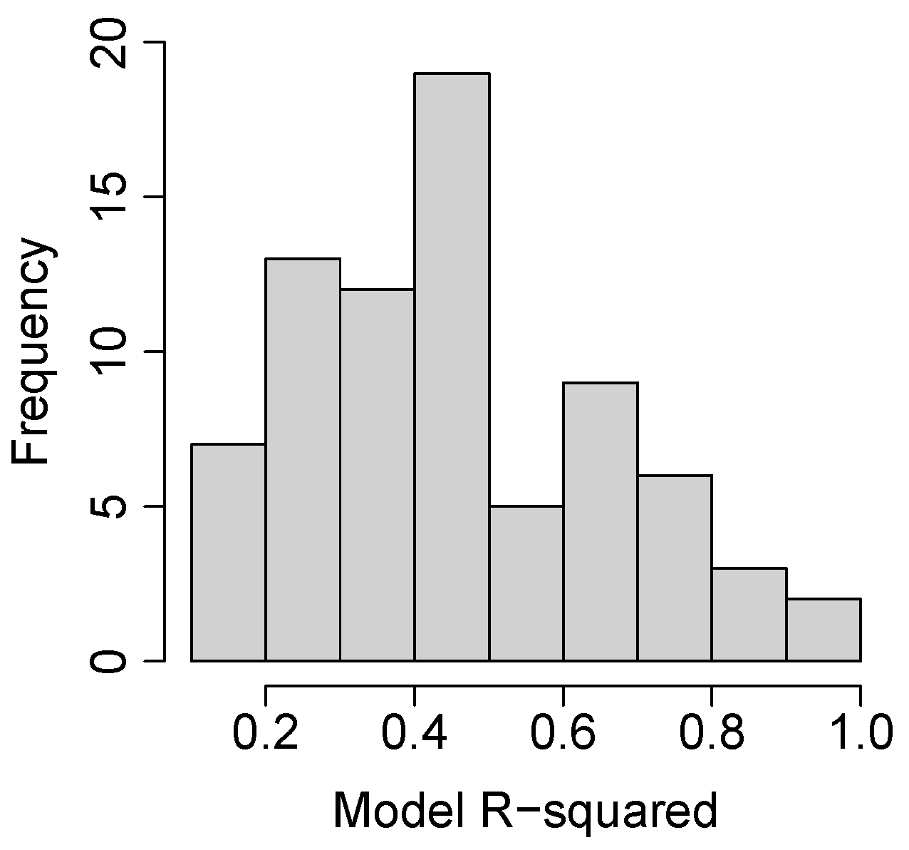
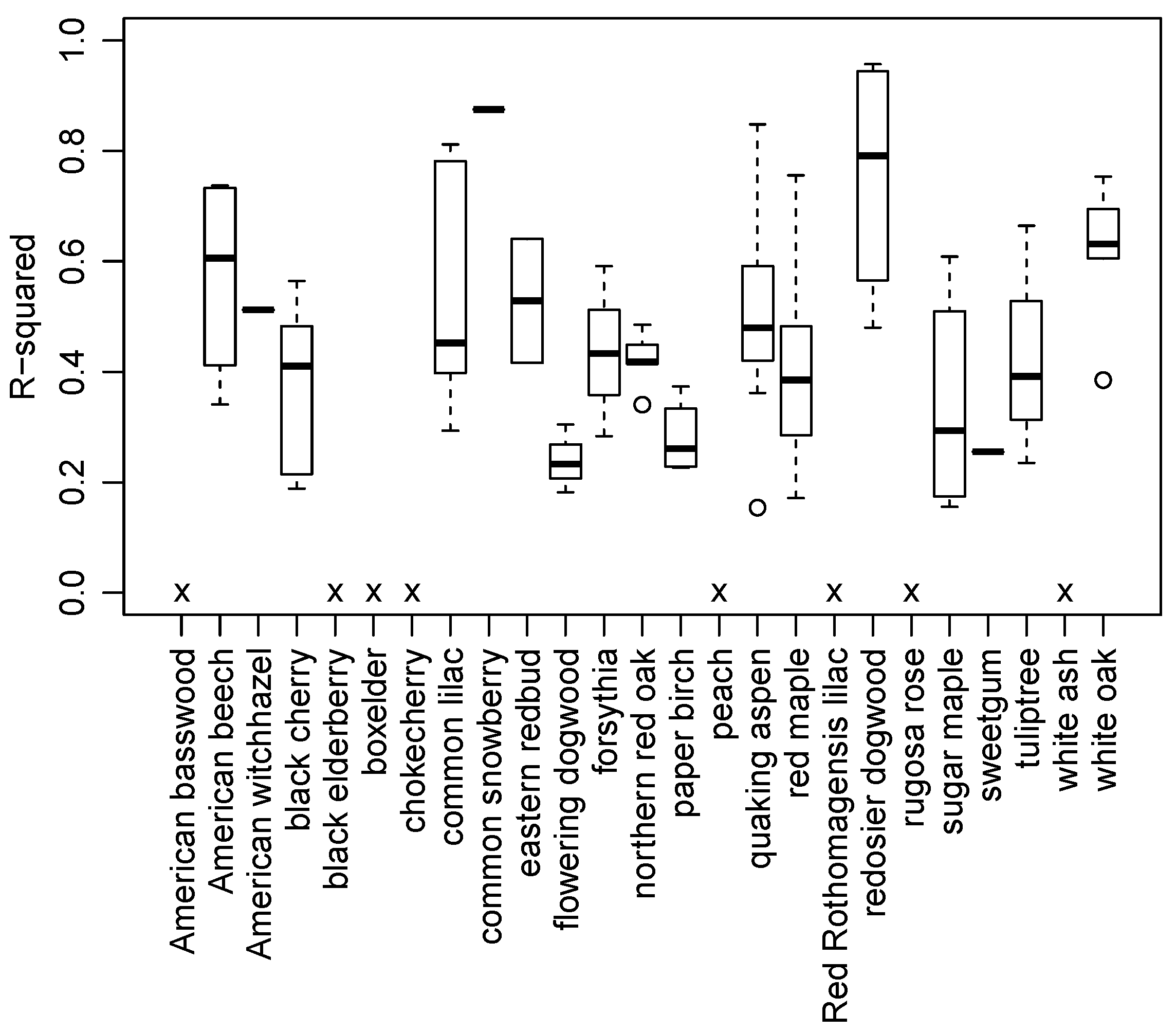
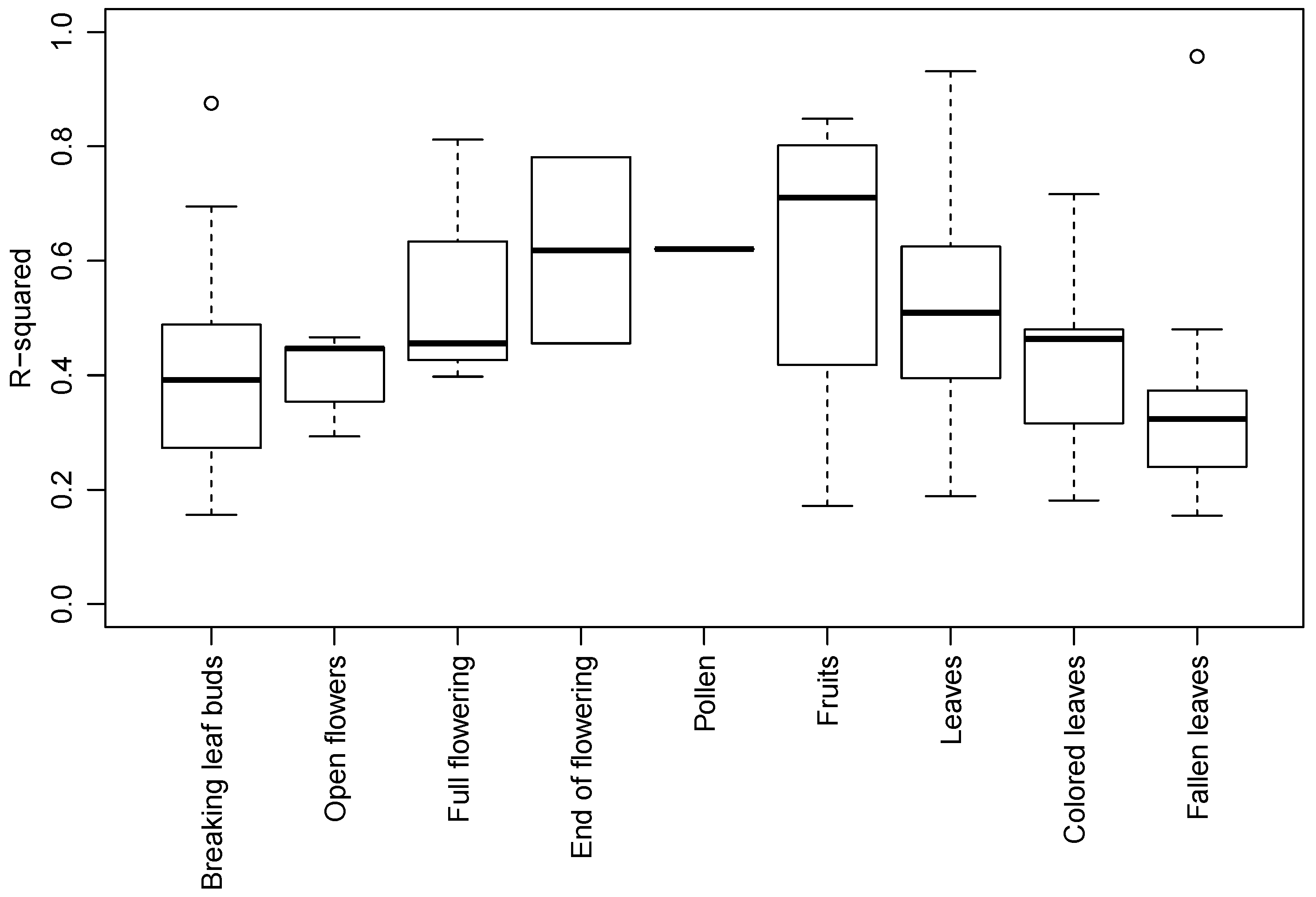
3.2. Species and Phenophase Model Variability

After all quality control steps were completed on data from all species-phenophase combinations, the final database included 4637 pairs of NN and MODIS records. This included multiple records of the same plant (e.g., records of flowers and leaves on one plant are recorded as two separate records). For each species-phenophase combination, observations spanned one to five years, one to 27 sites, and one to 106 observations. All NN spring phenophases were used in models with both MODIS spring phenophases (OGI and OGMax), and all NN autumn phenophases were used in models with both MODIS autumn phenophases (OGD and OGMin). This resulted in 228 models. Of these, 105 were significant (p < 0.05) (Table S2). The R2 of significant models ranged from 0.10 to 1.0. We observed that the model R2 decreased with increasing number of observations (R2 = 0.32; p < 0.001), but models with a very small sample size (e.g., <10 observations) and a high R2 influenced this result. After limiting the analysis to regressions with a sample size ≥10 (76 models; Table S2), the distribution of R2 values ranged from 0.1 to 0.95 and peaked near 0.4 (Figure 5) and there was no remaining correlation between sample size and model R2 (p = 0.236).
We grouped the model results by phenophase (NN and MODIS), species, and canopy position and tested for differences between group means. There was no difference in the mean R2 between models formed using each of the 4 MODIS phenophases, either across all phenopheses or within any one NN phenophase (p > 0.05). However, the number of significant models for each of the four MODIS phenophases was 28, 24, 7 and 20 for OGI, OGMax, OGD, OGMin, respectively. The low number of significant models for OGD suggests poorer performance overall for this measure of MODIS phenology. Additionally, for five of the nine NN phenophases (Leaves, open flowers, full flowering, end of flowering, and fruits), MODIS OGI produced the highest R2. Across species, there was a wide variability in R2 values, with mean R2 ranging from 0.23 to 0.89 (Figure 6). TukeyHSD tests showed no significant differences between species mean R2 (p > 0.05), but nine species returned no significant models with a sample size ≥10. Across all NN phenophases, mean R2 values ranged from 0.32 to 0.71 (Figure 7). The highest mean correlation (across all species) was exhibited by the ‘Fruits’ phenophase (R2 = 0.71), and the lowest was exhibited by fallen leaves (R2 = 0.32). There were no significant differences between model performances for the different NN phenophases.
Although the success of the different NN phenophases to correlate with MODIS varied between and within species, there were 11 species-phenophase combinations that resulted in models with R2 > 0.70 (Table S2) and 20 models with R2 > 0.60. Observations in this larger group of models (R2 > 0.60) included most of the phenophases, but missing were observations of open flowers. Leaves accounted for the highest proportion of models with R2 > 0.60. The regression with the largest number of observations was red maple leaves, which resulted in a model with R2 = 0.51. However, some of the most impressive models were formed using NN observations of leaves of other forest trees that often dominate forest stands, such as white oak (R2 = 0.71) and American beech (R2 = 0.73). Additionally, in some cases these observations of leaves formed strong relationships with several different MODIS phenophases (Table S2). The distribution of R2 values for tree species grouped by canopy position exhibited no significant differences between groups (p > 0.05; Figure 8) with the exception of redosier dogwood, which exhibited a higher R2 than flowering dogwood, paper birch or sugar maple (p < 0.05).

4. Discussion

4.1. Comparing Observations across Scales

As discussed in the Introduction, the relatively large areas covered by each MODIS pixel (250,000 m2) means the phenology of many individual plants residing in potentially very different habitats is integrated within each MODIS phenology observation. Many NN observations are made in sub-urban or even urban settings, and as discussed, we found that in many cases there were no forested MODIS pixels near these locations. The exercise of calculating the median phenology of all forested MODIS pixels successfully improved all of the regression model results reported here. This success is consistent with the idea that forested pixels represent the NN observations of tree and shrub phenology (even those plants growing outside of forests) more-readily than mixed land use pixels. Certainly microclimatic differences between urban, sub-urban and forested settings will influence the phenology of plants [35], but our work shows that field observations made in mixed land-use settings would still be useful for understanding climatic controls on spring phenology of nearby forest stands.
The phenology of forested MODIS pixels, as opposed to mixed-landuse pixels, correlated more highly with NN observations for a wide variety of species and phenophases. This is perhaps a bit unexpected in that greenness transitions were used to define all four MODIS phenophases, and we would expect a priori that the NN leaves phenophase would be more directly comparable to land surface phenology, upon which greenness transitions are the dominant influence. Lilac was perhaps the best example of a strong correlation between a flowering phenophase and MODIS phenology. Lilacs largely grow in locations that are convenient to observe (e.g., suburban yards), yet when forested MODIS pixels are located adjacent to these locations (an occurrence that happened just 30% of the time), we observed a strong correlation between full flowering phenology and MODIS phenology (R2 = 0.73). Overall, these results clearly support the continued use of lilac as a calibration species for volunteer observations of phenology, and despite the very different type of observation (e.g., flowering vs. land surface phenology), the strong correlation of these data provide validation of both observation types.
Previous work that has compared ground and remote sensing observations of phenology has emphasized that large remote sensing pixels represent the phenology of many species, each responding to different climatic cues [8,10,36]. It has also been found that remote sensing phenology is sensitive to the algorithm used [8] and efforts to link remote sensing phenology with models that predict phenology from meteorological data are highly sensitive to landscape variability inherent to temperate forests [37]. Why is it then that we found several species-phenophase combinations that correlated well with MODIS phenology? Benefits gained through careful data quality control should certainly be recognized (discussed below), but we also recognize that the phenology of certain species might better represent the average forest phenology at a particular location. This makes the most sense for dominant forest trees, such as white oak (R2 = 0.75) and American beech (R2 = 0.74), which logically contribute a large proportion of the signal to MODIS phenology observations. However, other less-dominant species that produced good correlations should also be considered good proxies for forest phenology in the landscapes they occupy. While good model performance might be serendipitous in some cases (i.e., when hundreds of models are formed, Type I errors potentially increase), it might also be valuable to examine if there are climatic origins to these patterns and if there are particular species that respond to similar climatic cues as the forest canopy as a whole. Such a result would not necessarily be surprising considering work indicating that the phenology of many species are behaving similarly to global change over time [38].

4.2. Recommendations for Phenology-Focused Citizen Science Efforts

Strong correlations between citizen scientists’ observations and MODIS provide confidence that both datasets have undergone sufficient quality control and assessment. This confidence is required before any further work with the data is attempted, such as evaluating trends over time in response to climate change. The quality control steps used here resulted in removing over 50% of NN observations, and the removal of non-forested pixels from the analysis had the largest effect on sample size and model performance. However, restricting observations to locations where adjacent forested pixels could be identified is only necessary when comparison with MODIS is a research goal. To enable future comparisons with remote sensing data, we recommend focusing future citizen science observations on the collection of data in fairly homogenous landscapes (e.g., from within interior forests) rather than diverse environments characterized by field-edges or sub-urban neighborhoods. This would be particularly useful for plants often found in forested landscapes. For example, in the NN protocol, volunteers are encouraged to select trees and shrubs for observation that are separated from buildings and roads, but not necessarily in forested areas. Citizen science efforts in general may be biased as volunteers may be more likely to collect data from more accessible locations, including those adjacent to roads and in residential landscapes [19]. Therefore, although the proximity to a forested pixel is directly relevant to the comparison with remote sensing, there are additional benefits that might be realized beyond this specific goal.
The quality control step of removing likely erroneous observations reported outside of a typical seasonal period had the smallest effect on sample size but a proportionally larger effect on model performance. Observations removed in this step are either erroneous (i.e., the phenophase was recorded incorrectly) or represent phenophase transitions that are due to atypical climatic conditions (e.g., an extremely warm autumn that causes leaf emergence). In an analysis of trends over time, neglecting this quality control step would risk the detection of a non-existent trend. However, if the detection of atypical conditions were the goal, this quality control step would not be best practice, because it would obviously mask the occurrence of the very events under study.
Requiring a maximum 10-day separation between the first ‘yes’ record and the previous ‘no’ record of each phenophase also increased the quality of the data obtained and is therefore highly recommended. Similarly, the authors of [19] suggest eliminating data from those who do not submit regularly, as well as those who lack experience. This data quality step is supported by recent research that emphasizes the value of repeated visits at regular intervals to ensure high-quality phenology data [39]. Stricter protocols, such as tracking phenology every 1–2 days, will provide more standardized data and possibly increased data quality but will make it difficult to recruit and retain volunteers. Training may help with such implementation; for example, the authors of [31] emphasized the importance of targeted and ongoing training, as well as regular feedback, to improve volunteers’ experience and reliability. Another possible solution is more relaxed requirements for most participants with more labor-intensive standardized sample for a small, but geographically dispersed, committed subset [19]. In any case, ongoing guidance and reminders are likely necessary to emphasize the importance of ‘no’ phenophase observations, as volunteers do not immediately realize its importance without explanation [33].

4.3. Could MODIS Be Used for High Throughput Phenotyping?

The observation that the MODIS phenology of forested pixels is correlated with volunteer observations of plants growing within or outside of forests suggests that MODIS phenology might be useful for predicting the phenology of individual plants. This is an important revelation because it opens the possibility of using remote sensing to identify plant phenotypes strongly related to climate change. The best correlations we observed included several important forest tree species, such as white oak, American beech, red maple, and poplar species. These relationships are approaching those necessary for predictions. For example, we calculated a prediction interval for the onset of the poplar leaves phenophase of ±15 days. The origin of variability within this interval is difficult to associate with any one mechanism, but we suspect it arises from uncertainty in volunteer observations of plant phenology, the algorithm used to fit a phenology curve to the MODIS data, and uncertainty in the underlying greenness observations themselves. For example, we conducted a simple stochastic simulation and found that if we round the date of occurrence of 100 random phenophase onset records to the nearest ten (e.g., DOY 115, 120, 124, and 128 would become DOY 110, 120, 120, and 120, respectively) we arrive at a prediction interval of ±11 days. If we further assume that in 10% of these cases the volunteer missed observing the phenophase on the first try, the prediction interval increases to ±15 days. On the other side of the coin, bootstrapped resampling of remote sensing vegetation data with repeated phenology curve fitting results in 95% confidence intervals of ±7 days [35]. As data density decreases (as would be the case with clouds or poor sun-sensor geometry), this measure of uncertainty increases. Therefore, there are clearly many sources of uncertainty in each data type that must be quantified and systematically addressed before routine predictions of sufficient accuracy will be possible [8,12].
If MODIS data are ever to be used to predict phenology of individual trees, our results point to some additional recommendations. Firstly, our work provides a list (Table S2) of species and phenotypes for which high throughput phenotyping via MODIS would be the most fruitful. Making this list are species like quaking aspen, which grows in large stands where it not only dominates at the species level but also maintains clonal (and phenological) homogeneity [40]. Overall, it appears that certain species are more representative of the average phenology of forests in the area, and therefore might be targeted for future work that utilizes remote sensing observations to measure the phenology of a single species over large geographic extents. Secondly, we recommend limiting predictions to MODIS spring phenophases, due to stronger correlations with NN ground observations in this season. In contrast, the onset of greenness decrease (an autumn phenophase) resulted in the fewest significant models, performing much worse than spring phenophase measures. This is consistent with past findings that spring phenophase observations correlate more strongly with ground-based observations than do autumn phenophase observations [34]. In remote sensing data, the autumn transitions are represented by a less rapid change in greenness that are harder to quantify [35], likely contributing to this effect. It is also possible that low light conditions characteristic of autumn degrade the remote sensing signal, thus reducing the quality of phenology observations.
While we only evaluated the correlation between NN and MODIS observations of phenology, we suspect our conclusions would extend to other citizen science efforts and other satellite systems. Remote sensing offers many options for measuring phenology that were not evaluated here. For example, flowering can be directly observed if high-resolution multi- or hyper-spectral imagery is available at the right time of year (e.g., [41]). Red leaf color, on the other hand, can be observed in medium to moderate resolution multispectral data [35], and future work might evaluate the potential of these remote observations to predict field-based observations. Active remote sensing systems, such as light detection and ranging (LiDAR) and synthetic aperture RADAR, as well as passive microwave sensors, have the added capability to detect leaf presence and absence, without regard to leaf color (e.g., [42,43]). By broadening the suite of remote sensing technologies brought to the problem, future work has the potential to further refine our understanding of precision and accuracy in both volunteer citizen science and remote sensing observations of phenology. These technologies might also aid in the quantitative scaling between remote- and ground-based observations.

5. Conclusions

Large MODIS pixels will always be an integration of many individual plants and diverse land cover, and this will limit compatibility with ground-based observations of phenology. However, we found that phenology estimates made from pixels centered on contiguous forest were highly correlated with ground-based citizen scientists’ observations, and that this result held for a wide variety of species and phenophases. Correlated ground- and remote observations provide confidence in both observation types, indicating success in the removal of outlier data as well as potentially supporting conclusions related to climatic controls on phenology. This result highlights the importance of citizen science to advance environmental research, while also opening possibilities for using forests as a proxy for the phenology of individual plants and complementing previous work that focused comparisons of remote sensing phenology with ground-based measures of average forest phenology. Additional components of successful cross-scalar comparisons were found to be the removal of volunteer observations outside of an acceptable window, and removing ‘yes’ records that were not preceded by ‘no’ records within an acceptable time period. While there are remaining uncertainties to resolve, we remain optimistic that remote sensing of phenology can be used in tandem with citizen scientists’ observations to characterize plant phenology over a range of geographic scales. The applications that this pairing of techniques will unlock is truly impressive and is poised in particular to make major contributions to understanding the response of forest plants to future changes in climate.

Supplementary Materials

The following are available online at www.mdpi.com/2072-4292/8/6/502/s1, Table S1: Species-specific temporal thresholds for acceptable spring and autumn observations, and the threshold number of days since a previous ’no’ observation; Table S2: Model results for all species-phenophase combinations, including non-significant models and models constructed from less than 10 observations.

Acknowledgments

We thank Theresa Crimmins for logistical support and for providing helpful comments during this project. This work is supported by the National Science Foundation (Grant #1461868).

Author Contributions

A.J.E. and C.S. conceived and designed the experiments; A.J.E. and K.P. analyzed the data; A.J.E. and K.P. contributed analysis tools; A.J.E. and C.S. wrote the paper.

Conflicts of Interest

The authors declare no conflict of interest. The founding sponsors had no role in the design of the study; in the collection, analyses, or interpretation of data; in the writing of the manuscript, and in the decision to publish the results.

Abbreviations

The following abbreviations are used in this manuscript:
DOYDay of Year
MODISModerate Resolution Imaging Spectrometer
NNNatures Notebook
NPNNational Phenology Network
OGDOnset of Greenness Decrease
OGIOnset of Greenness Increase
OGMaxOnset of Greenness Maximum
OGMinOnset of Greenness Minimum
LiDARLight Detection and Ranging
RADARRAdio Detection and Ranging

References

  1. Richardson, A.D.; Keenan, T.F.; Migliavacca, M.; Ryu, Y.; Sonnentag, O.; Toomey, M. Climate change, phenology, and phenological control of vegetation feedbacks to the climate system. Agric. For. Meteorol. 2013, 169, 156–173. [Google Scholar] [CrossRef]
  2. Xu, L.; Myneni, R.B.; Chapin, F.S., III; Callaghan, T.V.; Pinzon, J.E.; Tucker, C.J.; Zhu, Z.; Bi, J.; Ciais, P.; Tommervik, H.; et al. Temperature and vegetation seasonality diminishment over northern lands. Nat. Clim. Chang. 2013, 3, 581–586. [Google Scholar] [CrossRef]
  3. Keenan, T.F.; Gray, J.; Friedl, M.A.; Toomey, M.; Bohrer, G.; Hollinger, D.Y.; Munger, J.W.; O’Keefe, J.; Schmid, H.P.; Wing, I.S.; et al. Net carbon uptake has increased through warming-induced changes in temperate forest phenology. Nat. Clim. Chang. 2014, 4, 598–604. [Google Scholar] [CrossRef]
  4. Myneni, R.B.; Keeling, C.D.; Tucker, C.J.; Asrar, G.; Nemani, R.R. Increased plant growth in the northern high latitudes from 1981 to 1991. Nature 1997, 386, 698–702. [Google Scholar] [CrossRef]
  5. Schwartz, M.D.; Reiter, B.E. Changes in North American spring. Int. J. Climatol. 2000, 20, 929–932. [Google Scholar] [CrossRef]
  6. Cleland, E.E.; Chuine, I.; Menzel, A.; Mooney, H.A.; Schwartz, M.D. Shifting plant phenology in response to global change. Trends Ecol. Evolut. 2007, 22, 357–365. [Google Scholar] [CrossRef] [PubMed]
  7. Chuine, I.; Belmonte, J.; Mignot, A. A modelling analysis of the genetic variation of phenology between tree populations. J. Ecol. 2000, 88, 561–570. [Google Scholar] [CrossRef]
  8. White, M.A.; de Beurs, K.M.; Didan, K.; Inouye, D.W.; Richardson, A.D.; Jensen, O.P.; O’Keefe, J.; Zhang, G.; Nemani, R.R.; van Leeuwen, W.J.D.; et al. Intercomparison, interpretation, and assessment of spring phenology in North America estimated from remote sensing for 1982–2006. Glob. Chang. Biol. 2009, 15, 2335–2359. [Google Scholar] [CrossRef]
  9. Liang, L.; Schwartz, M. Landscape phenology: An integrative approach to seasonal vegetation dynamics. Landsc. Ecol. 2009, 24, 465–472. [Google Scholar] [CrossRef]
  10. Liang, L.A.; Schwartz, M.D.; Fei, S.L. Validating satellite phenology through intensive ground observation and landscape scaling in a mixed seasonal forest. Remote Sens. Environ. 2011, 115, 143–157. [Google Scholar] [CrossRef]
  11. Melaas, E.K.; Friedl, M.A.; Zhu, Z. Detecting interannual variation in deciduous broadleaf forest phenology using Landsat TM/ETM plus data. Remote Sens. Environ. 2013, 132, 176–185. [Google Scholar] [CrossRef]
  12. Liang, L.; Schwartz, M.D.; Wang, Z.S.; Gao, F.; Schaaf, C.B.; Tan, B.; Morisette, J.T.; Zhang, X.Y. A cross comparison of spatiotemporally enhanced springtime phenological measurements from satellites and ground in a Northern U.S. Mixed forest. IEEE Trans. Geosci. Remote Sens. 2014, 52, 7513–7526. [Google Scholar] [CrossRef]
  13. Keller, S.R.; Levsen, N.; Olson, M.S.; Tiffin, P. Local adaptation in the flowering-time gene network of balsam poplar, Populus balsamifera L. Mol. Biol. Evolut. 2012, 29, 3143–3152. [Google Scholar] [CrossRef] [PubMed]
  14. Olson, M.S.; Levsen, N.; Soolanayakanahally, R.Y.; Guy, R.D.; Schroeder, W.R.; Keller, S.R.; Tiffin, P. The adaptive potential of Populus balsamifera L. to phenology requirements in a warmer global climate. Mol. Ecol. 2013, 22, 1214–1230. [Google Scholar] [CrossRef] [PubMed]
  15. Savolainen, O.; Pyhajarvi, T.; Knurr, T. Gene flow and local adaptation in trees. Annu. Rev. Ecol. Evolut. Syst. 2007, 38, 595–619. [Google Scholar] [CrossRef]
  16. Hamunyela, E.; Verbesselt, J.; Roerink, G.; Herold, M. Trends in spring phenology of western European deciduous forests. Remote Sens. 2013, 5, 6159–6179. [Google Scholar] [CrossRef]
  17. Schwartz, M.D.; Hanes, J.M. Intercomparing multiple measures of the onset of spring in eastern North America. Int. J. Climatol. 2009, 30, 1614–1626. [Google Scholar] [CrossRef]
  18. Craine, J.M.; Battersby, J.; Elmore, A.J.; Jones, A.W. Building EDENs: The rise of environmentally distributed ecological networks. Bioscience 2007, 57, 45–54. [Google Scholar] [CrossRef]
  19. Dickinson, J.L.; Zuckerberg, B.; Bonter, D.N. Citizen science as an ecological research tool: Challenges and benefits. Annu. Rev. Ecol. Evolut. Syst. 2010, 41, 149–172. [Google Scholar] [CrossRef]
  20. Cooper, C.B.; Hochachka, W.M.; Dhondt, A.A. The opportunities and challenges of citizen science as a tool for ecological research. In Citizen Science: Public Collaboration in Environmental Research; Cornell University Press: Ithaca, NY, USA, 2011; pp. 99–113. [Google Scholar]
  21. Denny, E.G.; Gerst, K.L.; Miller-Rushing, A.J.; Tierney, G.L.; Crimmins, T.M.; Enquist, C.A.F.; Guertin, P.; Rosemartin, A.H.; Schwartz, M.D.; Thomas, K.A.; et al. Standardized phenology monitoring methods to track plant and animal activity for science and resource management applications. Int. J. Biometeorol. 2014, 58, 591–601. [Google Scholar] [CrossRef] [PubMed]
  22. Shirk, J.L.; Ballard, H.L.; Wilderman, C.C.; Phillips, T.; Wiggins, A.; Jordan, R.; McCallie, E.; Minarchek, M.; Lewenstein, B.V.; Krasny, M.E.; et al. Public participation in scientific research: A framework for deliberate design. Ecol. Soc. 2012, 17. [Google Scholar] [CrossRef]
  23. Bonney, R.; Shirk, J.L.; Phillips, T.B.; Wiggins, A.; Ballard, H.L.; Miller-Rushing, A.J.; Parrish, J.K. Next steps for citizen science. Science 2014, 343, 1436–1437. [Google Scholar] [CrossRef] [PubMed]
  24. Bird, T.J.; Bates, A.E.; Lefcheck, J.S.; Hill, N.A.; Thomson, R.J.; Edgar, G.J.; Stuart-Smith, R.D.; Wotherspoon, S.; Krkosek, M.; Stuart-Smith, J.F.; et al. Statistical solutions for error and bias in global citizen science datasets. Biol. Conserv. 2014, 173, 144–154. [Google Scholar] [CrossRef]
  25. Fitzpatrick, M.C.; Preisser, E.L.; Ellison, A.M.; Elkinton, J.S. Observer bias and the detection of low-density populations. Ecol. Appl. 2009, 19, 1673–1679. [Google Scholar] [CrossRef] [PubMed]
  26. Delaney, D.G.; Sperling, C.D.; Adams, C.S.; Leung, B. Marine invasive species: Validation of citizen science and implications for national monitoring networks. Biol. Invasions 2008, 10, 117–128. [Google Scholar] [CrossRef]
  27. Edgar, G.J.; Barrett, N.S.; Morton, A.J. Biases associated with the use of underwater visual census techniques to quantify the density and size-structure of fish populations. J. Exp. Mar. Biol. Ecol. 2004, 308, 269–290. [Google Scholar] [CrossRef]
  28. Fuccillo, K.K.; Crimmins, T.M.; de Rivera, C.E.; Elder, T.S. Assessing accuracy in citizen science-based plant phenology monitoring. Int. J. Biometeorol. 2014. [Google Scholar] [CrossRef] [PubMed]
  29. Edgar, G.J.; Stuart-Smith, R.D. Ecological effects of marine protected areas on rocky reef communities—A continental-scale analysis. Mar. Ecol. Prog. Ser. 2009, 388, 51–62. [Google Scholar] [CrossRef]
  30. Danielsen, F.; Jensen, P.M.; Burgess, N.D.; Altamirano, R.; Alviola, P.A.; Andrianandrasana, H.; Brashares, J.S.; Burton, A.C.; Coronado, I.; Corpuz, N.; et al. A multicountry assessment of tropical resource monitoring by local communities. Bioscience 2014, 64, 236–251. [Google Scholar] [CrossRef]
  31. See, L.; Comber, A.; Salk, C.; Fritz, S.; van der Velde, M.; Perger, C.; Schill, C.; McCallum, I.; Kraxner, F.; Obersteiner, M. Comparing the quality of crowdsourced data contributed by expert and non-experts. PLoS ONE 2013, 8. [Google Scholar] [CrossRef]
  32. Crimmins, T.M.; Crimmins, M.A.; Bertelsen, C.D. Flowering range changes across an elevation gradient in response to warming summer temperatures. Glob. Chang. Biol. 2009, 15, 1141–1152. [Google Scholar] [CrossRef]
  33. Crimmins, T.M.; Weltzin, J.F.; Rosemartin, A.H.; Surina, E.M.; Marsh, L.; Denny, E.G. Focused campaign increases activity among participants in nature’s notebook, a citizen science project. Nat. Sci. Educ. 2014, 43, 64–72. [Google Scholar]
  34. Ganguly, S.; Friedl, M.A.; Tan, B.; Zhang, X.; Verma, M. Land surface phenology from MODIS: Characterization of the collection 5 global land cover dynamics product. Remote Sens. Environ. 2010, 114, 1805–1816. [Google Scholar] [CrossRef]
  35. Elmore, A.J.; Guinn, S.M.; Minsley, B.J.; Richardson, A.D. Landscape controls on the timing of spring, autumn, and growing season length in mid-Atlantic forests. Glob. Chang. Biol. 2012, 18, 656–674. [Google Scholar] [CrossRef]
  36. Fisher, J.I.; Mustard, J.F. Cross-scalar satellite phenology from ground, Landsat, and MODIS data. Remote Sens. Environ. 2007, 109, 261–273. [Google Scholar] [CrossRef]
  37. Fisher, J.I.; Richardson, A.D.; Mustard, J.F. Phenology model from surface meteorology does not capture satellite-based greenup estimations. Glob. Chang. Biol. 2007, 13, 707–721. [Google Scholar] [CrossRef]
  38. Yue, X.; Unger, N.; Keenan, T.F.; Zhang, X.; Vogel, C.S. Probing the past 30-year phenology trend of US deciduous forests. Biogeosciences 2015, 12, 4693–4709. [Google Scholar] [CrossRef]
  39. Rosemartin, A.H.; Denny, E.G.; Weltzin, J.F.; Lee Marsh, R.; Wilson, B.E.; Mehdipoor, H.; Zurita-Milla, R.; Schwartz, M.D. Lilac and honeysuckle phenology data 1956–2014. Sci. Data 2015, 2, 150038. [Google Scholar] [CrossRef] [PubMed]
  40. Madritch, M.D.; Greene, S.L.; Lindroth, R.L. Genetic mosaics of ecosystem functioning across aspen-dominated landscapes. Oecologia 2009, 160, 119–127. [Google Scholar] [CrossRef] [PubMed]
  41. Andrew, M.E.; Ustin, S.L. Effects of microtopography and hydrology on phenology of an invasive herb. Ecography 2009, 32, 860–870. [Google Scholar] [CrossRef]
  42. Frolking, S.; Milliman, T.; McDonald, K.; Kimball, J.; Zhao, M.S.; Fahnestock, M. Evaluation of the seawinds scatterometer for regional monitoring of vegetation phenology. J. Geophys. Res.-Atmos. 2006, 111. [Google Scholar] [CrossRef]
  43. Jones, M.O.; Kimball, J.S.; Jones, L.A.; McDonald, K.C. Satellite passive microwave detection of North America start of season. Remote Sens. Environ. 2012, 123, 324–333. [Google Scholar] [CrossRef]
Figure 1. The relationship between the number of observations retained and the threshold minimum number of days between the first ‘yes’ record and the previous ‘no’ record.
Remotesensing 08 00502 g001
Figure 2. Scatter plots of MODIS OGI vs. NN leaves observations for poplar at different stages of analysis. (A) Before any quality control; (B) after excluding observations outside the acceptable temporal window; (C) after excluding ‘yes’ records without a preceeding ‘no’ record within the previous 10 days; and (D) after adopting the median MODIS OGI for forested pixels surrounding each site as the MODIS measure of OGI.
Remotesensing 08 00502 g002
Figure 3. Scatter plots comparing MODIS OGI with the (A) Breaking leaf buds; (B) Leaves; (C) Open flowers; (D) Full flowering; (E) Pollen; and (F) Fruits NN phenophases for poplar (quaking aspen and balsam poplar combined).
Remotesensing 08 00502 g003
Figure 4. Scatter plots comparing MODIS OGI with the (A) Breaking leaf buds; (B) Leaves; (C) Open flowers; (D) Full flowering; and (E) End of flowering NN phenophases for lilac.
Remotesensing 08 00502 g004
Figure 5. Histogram of R2 values for significant models with observations ≥10.
Remotesensing 08 00502 g005
Figure 6. Boxplot showing mean and variance of R2 values resulting from all models between NN observations and MODIS with ≥10 observations. Models are grouped by species; missing catagories (denoted with an ‘x’) result from the lack of any significant models with ≥10 observations. There were no significant differences (Tukey HSD) between any pair of species with the exception of species with no significant models, and between redosier dogwood (high R2) and three species with low mean R2 (flowering dogwood, paper birch, and sugar maple) (p < 0.05).
Remotesensing 08 00502 g006
Figure 7. Boxplot showing mean and variance of R2 values resulting from all models between NN observations and MODIS phenology with observations ≥10. Models are grouped by NN phenophase. There are no significant differences between any pair of NN phenophases (Tukey HSD).
Remotesensing 08 00502 g007
Figure 8. Boxplot showing mean and variance of R2 values resulting from all models between NN observations and MODIS phenology with ≥10 observations. Models are grouped by life form. As the letters above each box show, the mean model R2 for tall trees was higher than that for short trees.
Remotesensing 08 00502 g008
Table 1. Study species meeting criteria described in the methods.
SpeciesCommon NameLife Form
Acer negundoboxelderLower canopy tree
Acer rubrumred mapleUpper canopy tree
Acer saccharumsugar mapleUpper canopy tree
Betula papyriferapaper birchUpper canopy tree
Cercis canadensiseastern redbudLower canopy tree
Cornus floridaflowering dogwoodLower canopy tree
Cornus sericearedosier dogwoodShrub
Fagus grandifoliaAmerican beechUpper canopy tree
Forsythia × intermediaforsythiaShrub
Fraxinus americanawhite ashUpper canopy tree
Hamamelis virginianaAmerican witchhazelLower canopy tree
Liquidambar styracifluasweetgumUpper canopy tree
Liriodendron tulipiferatuliptreeUpper canopy tree
Populus tremuloidesquaking aspenUpper canopy tree
Prunus persicapeachLower canopy tree
Prunus serotinablack cherryUpper canopy tree
Prunus virginianachokecherryShrub
Quercus albawhite oakUpper canopy tree
Quercus rubranorthern red oakUpper canopy tree
Rosa rugosarugosa roseShrub
Sambucus nigrablack elderberryShrub
Symphoricarpos albuscommon snowberryShrub
Syringa vulgariscommon lilacShrub
Syringa × chinensisRed Rothomagensis lilacShrub
Tilia americanaAmerican basswoodUpper canopy tree

