Defuzzification Strategies for Fuzzy Classifications of Remote Sensing Data

Abstract

The classes in fuzzy classification schemes are defined as fuzzy sets, partitioning the feature space through fuzzy rules, defined by fuzzy membership functions. Applying fuzzy classification schemes in remote sensing allows each pixel or segment to be an incomplete member of more than one class simultaneously, i.e., one that does not fully meet all of the classification criteria for any one of the classes and is member of more than one class simultaneously. This can lead to fuzzy, ambiguous and uncertain class assignation, which is unacceptable for many applications, indicating the need for a reliable defuzzification method. Defuzzification in remote sensing has to date, been performed by “crisp-assigning” each fuzzy-classified pixel or segment to the class for which it best fulfills the fuzzy classification rules, regardless of its classification fuzziness, uncertainty or ambiguity (maximum method). The defuzzification of an uncertain or ambiguous fuzzy classification leads to a more or less reliable crisp classification. In this paper the most common parameters for expressing classification uncertainty, fuzziness and ambiguity are analysed and discussed in terms of their ability to express the reliability of a crisp classification. This is done by means of a typical practical example from Object Based Image Analysis (OBIA).

1. Introduction

In contrast to crisp classification methods, which assign pixels or segments to disjoint classes in an exclusive manner, fuzzy classification methods generate gradual memberships of pixels or segments to one or more classes, which can be overlapping in feature space. This allows (a) the uncertainty of a particular class assignment to be explicitly expressed as a function of the degree of fulfilment of the underlying classification rules and (b) pixels or segments to be assigned to more than one class but with varying degrees of membership. While the former allows the handling of imprecise, incomplete or vague data for classification, the latter allows pixels or segments to gain an intermediate or transitional state of classification, such as mixed pixels [1,2,3]. Fuzziness as a further criterion to evaluate a classification’s reliability expresses the general clarity of a pixel’s or segment’s (multiple) fuzzy classification result(s) [4,5]. With the advent of Object Based Image Analysis (OBIA), fuzzy classification methods have been applied in a variety of remote sensing applications, whereby hierarchical classification schemas became very popular [6,7] since they reflect the classes’ ontologies and thus increase the transparency of the classification process and its results. Fuzzy rule sets—generated explicitly or based on samples of the intended classes—can thus comprise of individually formulated expert knowledge for each application domain. However when analysing remote sensing data, users generally expect undoubtable and crisp classification results that meet pre-defined quality criteria, describing the classification’s correctness and completeness (ISO 19157:2013). In this context defuzzification plays a central role, since further usage of the classification results can only be applied to crisp assigned segments or pixels. Information concerning the certainty, fuzziness and ambiguity of defuzzified classification results is therefore important or at least highly desirable, since it supports the evaluation of the classifications’ quality by evaluating its reliability. It is against this background that different methods of evaluating the certainty, fuzziness and ambiguity of fuzzy classification results are analyzed in the present article, in order to support decision-making regarding whether or not to defuzzify individual classification results. By means of a rather simple but easy to comprehend classification example, the article demonstrates the interrelation between achievable classification reliability and the achievable area coverage of crisp classification results. Further, it demonstrates the interrelation between achievable reliability and the semantic level of detail of hierarchical classification schemes. Classification results that are not satisfyingly reliable or do not provide satisfying spatial comprehensiveness indicate that the intended classes cannot be satisfyingly detected with the given class descriptions and data. That is, the class definitions need to be reconsidered or the input data must be changed. The paper suggests strategies for defuzzification supporting navigation within a stress field that is spanned by: the classification’s reliability, its semantic richness and its completeness.

2. Materials and Methods

2.1. Fuzzy Classification of Remote Sensing Data

Image analysis of remote sensing data in most cases means to assign pixels or segments, also known as image objects, to semantically meaningful land cover classes, according to implicitly or explicitly defined classification rules. In the following, pixels, segments and image objects will be termed ‘entity’ for simplicity reasons. That is, for every entity to be assigned to a particular class it must fulfil the criteria of the class definition, which is usually expressed by conditional terms in the form of: “IF <conditions> THEN <class>”, whereby several conditions can be combined by the logical operators AND and OR. Conditions combined by AND operators are only fulfilled if all of them are fulfilled, while those combined with the OR-operator are already fulfilled if at least one of them is fulfilled. AND and OR can be combined and nested according to the rules of Boolean algebra, allowing even complex classification rules to be defined. Performing a fuzzy classification means to define the desired land cover classes as fuzzy sets, using respective fuzzy membership functions for each classification condition, as outlined in [8]. That is, if the classification conditions for an entity are fulfilled only gradually, the membership to a particular class is also gradual. The degree of membership to a particular class A for an individual entity depends on the fuzzy-membership function(s) used and is expressed by ${\mathsf{\mu }}_A$, where ${\mathsf{\mu }}_A=0.0$ indicates that the required conditions for the entity to be a member of class A have not been satisfied; ${\mathsf{\mu }}_A=1.0$ indicates that these conditions have been fully satisfied. If the conditions are only partly satisfied ${\mathsf{\mu }}_A$ is ascribed a value between 0.0 and 1.0 [8].

A class A can be described by n fuzzy classification rules, defined as fuzzy-membership functions, which can be combined using the fuzzy-logical operators. The most popular operators in remote sensing are “fuzzy-AND” and “fuzzy-OR”. The fuzzy-AND operator yields the minimum of all membership values: ${\mathsf{\mu }}_A=min\left({\mathsf{\mu }}_{A,1},\dots ,{\mathsf{\mu }}_{A,n}\right)$ or the minimum t-norm, or ${⊺}_{min}\left({\mathsf{\mu }}_{A,1},\dots ,{\mathsf{\mu }}_{A,n}\right)$, while the fuzzy-OR operator yields the maximum value ${\mathsf{\mu }}_A=max\left({\mathsf{\mu }}_{A,1},\dots ,{\mathsf{\mu }}_{A,n}\right)$, or the maximum t-conorm or, ${\perp }_{max}\left({\mathsf{\mu }}_{A,1},\dots ,{\mathsf{\mu }}_{A,n}\right)$. Fuzzy-AND and fuzzy-OR rules can be combined and nested analogous to Boolean classification rules. A detailed discussion on fuzzy aggregation operators (t-norms and t-conorms) can be found in Yager [9]. Some of the operators presented there yield further opportunities for research in the context of remote sensing data analysis.

Fuzzy classified entities can be members of several classes simultaneously but with varying degrees of membership, that is, they fulfil the classification conditions of several classes with different grades. Such entities are regarded as being classified ambiguously. In order to calculate the fuzzy membership of each entity to all the classes of a classification scheme M with m classes, i.e., M = {A₁, A₂…A_m}, the Degree Of Fulfilment) (DOF_Ai) of the entity for each class is evaluated. In order to describe similarities between classes of M it can be organized hierarchically. In such a scheme M consists of node classes (N-classes) and leaf classes (L-classes). N-classes describe those characteristics all subsequent L-classes of an N-class have in common (Figure 1). That is, L-classes inherit the descriptions of their N-classes [10,11]. Entities can only be a member of a particular L-class if they fulfil the classification conditions of the L-classes’ N-classes and those of the L-class. That is, for an entity to be a member of a particular L-Class all DOF_N>0.0 and DOF_L>0.0 must be given. An entity’s membership degree to an L-class μ_L is then the minimum out of all DOF_N values (inherited descriptions) and the DOF_L value for that particular L-class. Hence, inheritance operates similar to the fuzzy-AND operator in a hierarchical fuzzy classification scheme, because an L-class member must satisfy the minimum requirements for all its N-classes and for the L-class:

$${\mathsf{\mu }}_L=\min \left(DO{F}_{N1},\dots DO{F}_{Nn}, DO{F}_L\right)$$

(1)

If M is not hierarchically organized, or A has no N-classes, for each entity its ${\mathsf{\mu }}_A=DO{F}_A$ (Figure 1).

Since an entity can be a gradual member of all L-classes and fulfil the classification conditions for all (L- and N-) classes of M, it has two vectors: $\overrightarrow{\mathsf{\mu }}$ and $\stackrel{\rightharpoonup }{DOF}$. Each of them contains m elements, which express the entity’s membership degrees to the L-classes and the $DOFs$ for each class of the scheme [10]:

$$\overrightarrow{\mathsf{\mu }}=\left({\mathsf{\mu }}_0, \dots , {\mathsf{\mu }}_m\right)$$

(2)

and

$$\stackrel{\rightharpoonup }{DOF}=\left(DO{F}_0, \dots , DO{F}_m\right)$$

(3)

An entity can therefore be a gradual member of several L-classes simultaneously but with different degrees of membership to each of them. An entity can likewise meet the classification conditions for several different classes simultaneously, allowing it to inherit the $DOFs$ of multiple classes.

2.2. Defuzzification of Fuzzy Classification Results

Several defuzzification methods for non-nominally scaled data have been proposed in published literature [12,13]. However, in remote sensing, crisp classification results are nominally scaled [14]. Defuzzification in remote sensing therefore means that ${\mathsf{\mu }}_A$ for each entity is converted from $\left[\mathrm{0..1}\right]\mathsf{ϵ}{ℝ}^{+}$ into ${\mathsf{\eta }}_{\mathrm{A}}\mathsf{ϵ}\left\{0,1\right\}$ with ${\mathsf{\eta }}_{\mathrm{A}}\mathsf{ϵ}\mathbb{N}$, where ${\mathsf{\eta }}_{\mathrm{A}}=0$ indicates that the entity of concern is not a member of class A, and ${\mathsf{\eta }}_{\mathrm{A}}=1$ indicates that it is a member of class A. Each entity is therefore usually assigned to the class for which it has the highest membership degree, that is, where ${\mathsf{\mu }}_{\mathrm{A}}=\max (\overrightarrow{\mathsf{\mu }})$. This class is often referred to as the Best Classification Result (BCR) [11,15], with ${\mathsf{\mu }}_{\text{BCR}}=\max (\overrightarrow{\mathsf{\mu }})$. A very simple but often applied method to defuzzify nominally scaled entities is to set a threshold t for ${\mathsf{\mu }}_{\text{BCR}}$: entities with ${\mathsf{\mu }}_{\text{BCR}}<\mathrm{t}$ remain unclassified, those with ${\mathsf{\mu }}_{\text{BCR}}\ge \mathrm{t}$ are assigned to BCR [6]. However, it is obvious that doubtful crisp classification results can be produced with this simple decision rule for the following reasons: (1) even those entities whose fuzzy memberships indicate little clarity of their class assignment can be crisp assigned to their BCR, that is, entities with ${\mathsf{\mu }}_{\text{BCR}}\cong 0.0$ (uncertainty); (2) entities whose ${\mathsf{\mu }}_{\text{BCR}}$ is similar to any of the remaining class memberships of $\overrightarrow{\mathsf{\mu }}$ (ambiguity) might be defuzzified; (3) entities whose ${\mathsf{\mu }}_{\text{BCR}}$ and all other class memberships indicate a high classification fuzziness (${\mathsf{\mu }}_{\text{BCR}}\cong {\mathsf{\mu }}_1\cong \dots \cong {\mathsf{\mu }}_{\mathrm{m}}\cong 0.5$) might be defuzzified.

2.2.1. Classification Uncertainty and Ambiguity

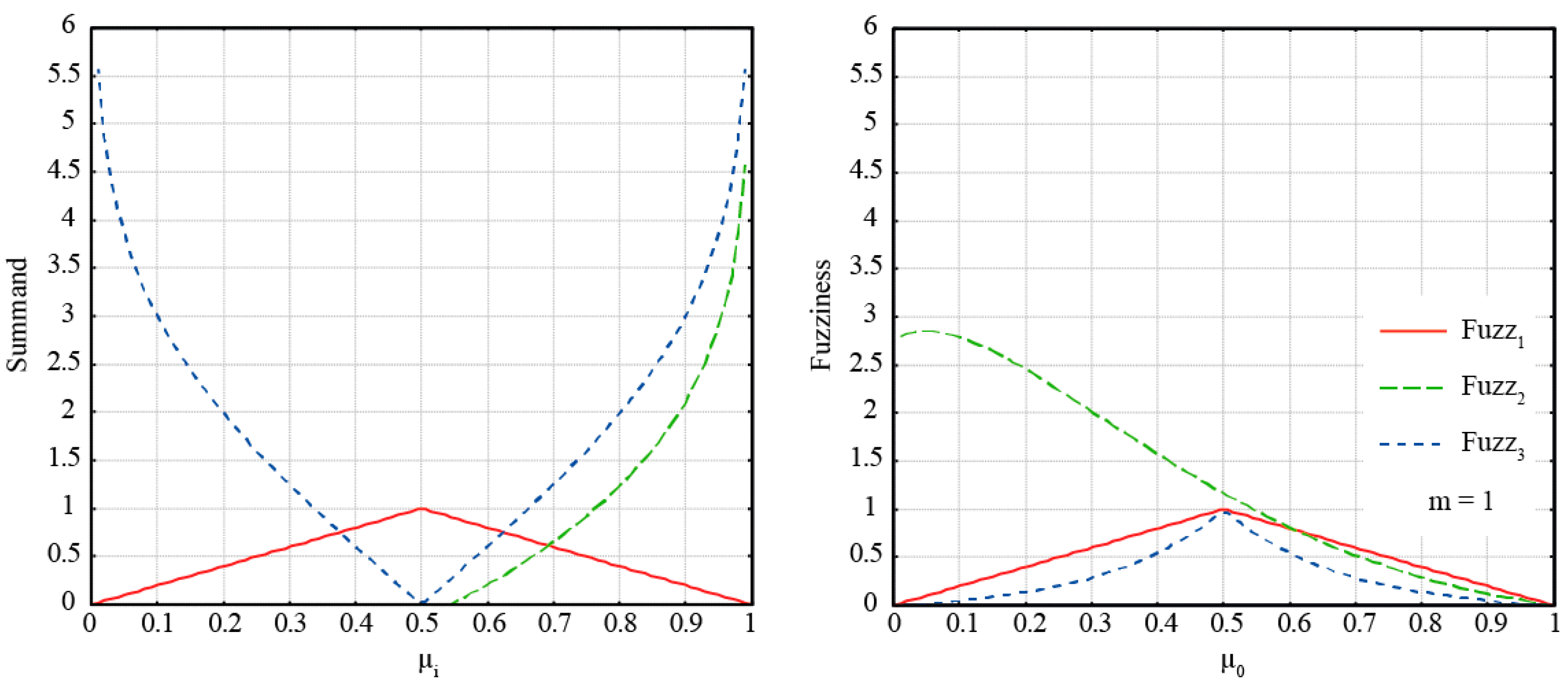
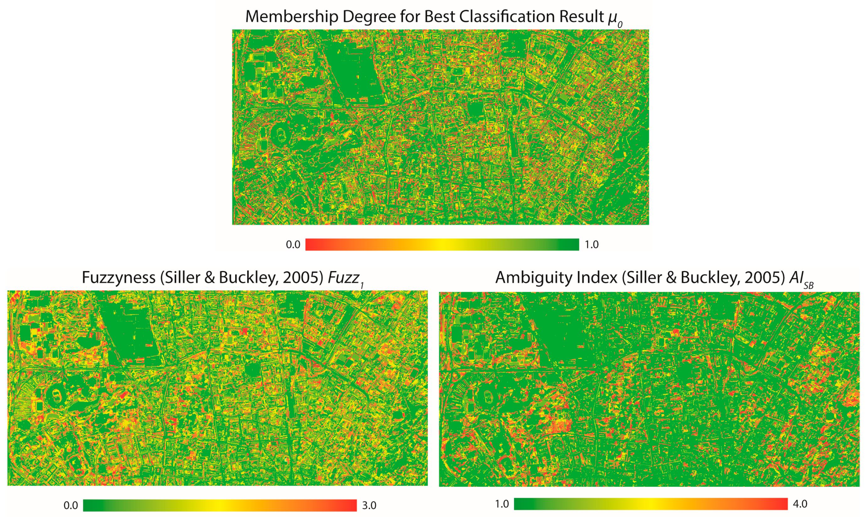
For each entity being fuzzy-classified using a classification scheme M, with m (L-)classes, the elements of its classification vector $\overrightarrow{\mathsf{\mu }}=\left({\mathsf{\mu }}_0,{\mathsf{\mu }}_1,\dots ,{\mathsf{\mu }}_{\mathrm{m}}\right)$ can be sorted following a “≥” relationship, beginning with ${\mathsf{\mu }}_{\text{BCR}}:{\mathsf{\mu }}_{\text{BCR}}\ge {\mathsf{\mu }}_{2\text{nd}}\ge \dots \ge {\mathsf{\mu }}_{\text{mth}}$, where ${\mathsf{\mu }}_{2\text{nd}}$ holds the membership degree of the second-best class and so on until the mth-best class. For better readability an index will be used here, to indicate the membership degree of an entity to its ith-best class with $i=0 \dots m$: ${\mathsf{\mu }}_0\ge {\mathsf{\mu }}_1 \ge \dots \ge {\mathsf{\mu }}_m$. Since the best possible membership degree an entity can have for an arbitrary class is ${\mathsf{\mu }}_{\mathrm{i}}=1.0$, the entity’s classification uncertainty can be expressed by: $1.0-{\mathsf{\mu }}_0$. An entity’s classification is ambiguous as soon as it has membership degrees of ${\mathsf{\mu }}_{\mathrm{i}=\mathrm{1..}\mathrm{m}}>0.0$ for any of the other classes in the classification scheme M [16,17]. Additionally, the ambiguity of an entity is considered higher, the closer all its ${\mathsf{\mu }}_i$ values are to each other. That is, in a “≥” order of membership degrees per entity, an entity with ${\mathsf{\mu }}_0\gg {\mathsf{\mu }}_1\gg \dots \gg {\mathsf{\mu }}_{\mathrm{m}}$ is less ambiguously classified than an entity with ${\mathsf{\mu }}_0\cong {\mathsf{\mu }}_1\cong \dots \cong {\mathsf{\mu }}_{\mathrm{m}}$. Consequently, quantifying and analysing the ambiguity and uncertainty for each fuzzy classified entity and setting meaningful thresholds to decide whether to defuzzify its fuzzy classification result or not, can make the crisp classification result as reliable as necessary.

2.2.2. Fuzziness

According to [5], fuzziness can be expressed by the separability of a fuzzy set and its complement. For fuzzy classifications in remote sensing this means: the clearer an arbitrary class A can be separated from its complementary class $\overline{A}$, the less fuzzy the class is. Siler & Buckley [4] transfer this to evaluate an entity’s classification fuzziness as follows: an entity is the less fuzzy assigned to a class or its complement, the closer its membership degree µ_A to this particular class is either to 1.0 or to 0.0. That is, an entity is the fuzzier assigned to A, the closer ${\mathsf{\mu }}_A=0.5$ and vice versa. When applying a fuzzy classification scheme M with several classes, as outlined before, this means an entity is the fuzzier classified, the more class memberships of ${\mathsf{\mu }}_i=0.5$ it has and it is fuzziest classified if all of the m memberships are ${\mathsf{\mu }}_i=0.5$. Besides minimizing an entity’s ambiguity and uncertainty, its fuzziness should be minimized too, in order to define sensible decision rules for the defuzzification of an entity’s fuzzy classification. Note: an entity with a membership degree of ${\mathsf{\mu }}_0=1.0$ and ${\mathsf{\mu }}_1=0.0$ simultaneously has the highest possible certainty and the lowest possible ambiguity and fuzziness.

2.2.3. Quantifying Classification Uncertainty, Ambiguity and Fuzziness per Entity

When determining the classification ambiguity, it is common in both published literature [6,15,18] and existing software (for example eCognition), for only the best and second-best class memberships to be evaluated. This is because for entities with ordinally scaled $\overrightarrow{\mathsf{\mu }}$ vectors, as soon as ${\mathsf{\mu }}_1>0.0$that entity’s classification is already ambiguous. However, measurement of the classification ambiguity becomes more precise if all membership degrees are taken into account but in this case, the degree of ambiguity is dependent on the number of classes m of a given classification scheme and can therefore be less easily compared with other classification schemes. In general, measures expressing an entity’s uncertainty, ambiguity and fuzziness should ideally be independent from m and easy to interpret. Some measures of uncertainty, ambiguity and fuzziness are discussed below. These measures were implemented using the Cognition Network Language (CNL) [19] and can be applied as a so-called “Customized Algorithm” in eCognition (see the relevant file, together with a short description of the “Customized Algorithm” in supplementary materials).

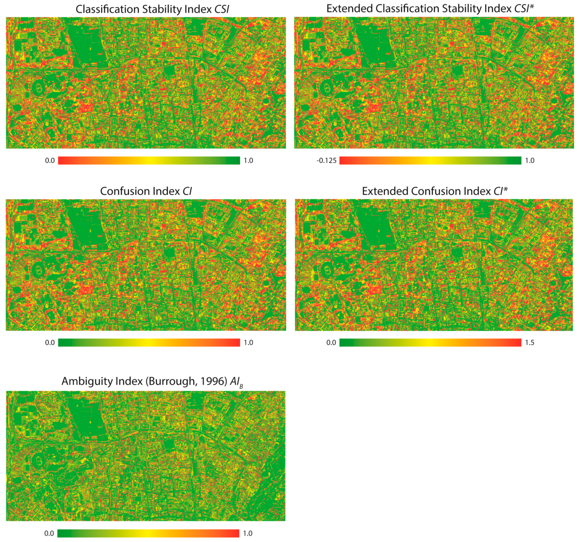
• Classification Stability Index and Confusion Index

The Classification Stability Index CSI, which is implemented in eCognition software as “Classification Stability” [11], expresses the difference between ${\mathsf{\mu }}_0$ and ${\mathsf{\mu }}_1$ for each entity. If $\overrightarrow{\mathsf{\mu }}$ is ordinally scaled [15] the CSI quantifies the entity’s ambiguity:

$$CSI={\mathsf{\mu }}_0-{\mathsf{\mu }}_1$$

(4)

where the value range of CSI is given by $0.0\le CSI\le 1.0$. The lower the CSI, the more ambiguous (less firm) an entity’s classification is. It takes into account ${\mu }_1$ only and none of the remaining µ_i of a classification. If all m class memberships of a given classification scheme are to be taken into account, the CSI extends to $CS{I}^{*}$:

$$CS{I}^{*}={\mathsf{\mu }}_0-{\sum }_{i=1}^m{\mathsf{\mu }}_i$$

(5)

The value range of CSI* is given by $1.0-m\le CS{I}^{*}\le 1.0$, which means that the CSI* can have negative values. Burrough [18] suggests the Confusion Index (CI) to express the ambiguity of an entity’s classification result, which is simply the compliment of the CSI. It can be calculated by:

$$CI=1.0-\left({\mathsf{\mu }}_0-{\mathsf{\mu }}_1\right)$$

(6)

with the value range of $0.0 \le CI \le 1.0$. That is, an entity is an increasingly distinct member of its BCR the lower the CI is. Analogous to the CSI, the CI can be extended to a more precise index by taking into account all m memberships of an entity to the classes of a given scheme:

$$C{I}^{*}=1.0-({\mathsf{\mu }}_0-({\sum }_{i=1}^m{\mathsf{\mu }}_i))$$

(7)

The value range of the $C{I}^{*}$ is then $0.0\le C{I}^{*}\le m$. Thus, it needs to be interpreted differently: the closer the $C{I}^{*}$ of an entity’s classification is to m, the less distinctly it is assigned to its BCR.

2.

Ambiguity Index

There have been different definitions proposed for the Ambiguity Index (AI). Burrough [18] defined it as the difference between the best possible classification result ${\mathsf{\mu }}_0=1.0$ and the best classification result actually achieved (${\mathsf{\mu }}_0$):

$$A{I}_B=1.0-{\mathsf{\mu }}_0$$

(8)

where the value range for $A{I}_B$ is given by $0.0\le A{I}_B\le 1.0$. This means: the less certain it is that an entity has been assigned to the best class, the more ambiguous its class assignment is. This parameter therefore measures the classification uncertainty of an entity, rather than its ambiguity. Siler & Buckley [4] instead suggested adding together all membership degree values achieved by an entity, divided by its best membership degree:

$$A{I}_{SB}={\sum }_{i=0}^m\frac{{\mathsf{\mu }}_i}{{\mathsf{\mu }}_0}$$

(9)

where the value range for $A{I}_{SB}$ is given by $1.\le A{I}_{SB}\le m$. $A{I}_{SB}$ takes into account an entity’s membership degree for all classes in a given classification scheme. However, as for the CS* and CI*, under this definition the index is dependent on m, while $A{I}_B$ is independent of m. In contrast to $A{I}_B$, $A{I}_{SB}$ truly measures the classification ambiguity: even if ${\mathsf{\mu }}_0$ for an entity is low, but the entity has only one single class assignment $A{I}_{SB}=1.0$. That is, the classification result for this particular entity might be uncertain but not ambiguous. Vice versa, the maximum ambiguity is achieved if all of the entity’s membership degrees are equal, independent of their grade, that is, if ${\mathsf{\mu }}_0={\mathsf{\mu }}_1=\dots ={\mathsf{\mu }}_m$. In case the entity of concern remains unclassified ${\mathsf{\mu }}_0=0.0$ and $A{I}_{SB}$ remains undefined.

3.

Fuzziness

Siler & Buckley [4] suggested quantifying the fuzziness of an entity’s classification by evaluating its number of class assignments with the highest possible fuzziness, that is, with a membership degree of ${\mathsf{\mu }}_i=0.5$. The more class assignments with ${\mathsf{\mu }}_i=0.5$ an entity has, the fuzzier its classification is. Consequently, the more class memberships with ${\mathsf{\mu }}_i=1.0$ or ${\mathsf{\mu }}_i=0.0$ an entity has, the less fuzzy it is classified. Membership degrees of $0.0<{\mathsf{\mu }}_i<0.5$ and $0.5<{\mathsf{\mu }}_i<1.0$ impact the accumulated fuzziness, respectively. They suggested two methods: a less precise method, with:

$$Fuz{z}_1={\sum }_{i=0}^{m}1.0-\left|\left(2{\mu }_i-1.0\right)\right|$$

(10)

where the value range for $Fuz{z}_1$ is given by $0.0\le Fuz{z}_1\le m$, and a more precise method, which is given and discussed in Appendix A. The latter is similar to the method suggested by de Luca & Termini [20]. However, although it is more precise, it is more sensitive when applying complex classification schemes with many classes: for the entity of concern a single membership to one of the scheme’s classes with ${\mathsf{\mu }}_i=0.0$ or ${\mathsf{\mu }}_i=1.0$ is already enough for this measure to equal its maximum or minimum value. In contrast, $Fuz{z}_1$ behaves continuously: it achieves its maximum if all class memberships yield ${\mathsf{\mu }}_i=0.5$, otherwise it decreases with the number of memberships ${\mathsf{\mu }}_i\ne 0.5$ per entity, whereas the closer the memberships are to 0.0 or 1.0 (${\mathsf{\mu }}_i\cong 0.0$ or ${\mathsf{\mu }}_i\cong 1.0$) per entity the more $Fuz{z}_1$ decreases. Nevertheless, none of the measures of fuzziness are capable of expressing an entity’s classification certainty or ambiguity. A detailed overview of fuzzy uncertainty and related discussions, has been provided by Pal & Bezdek [21].

2.2.4. Decision Rules for Defuzzification

Defuzzifying a fuzzy classification result of a given entity means to crisply assign it to its BCR. However, as already stated above, fuzzy classification results should only be defuzzified if the entity of concern is undoubtedly assignable to its BCR. In this context “undoubtedly” translates to: least uncertain, least ambiguous and least fuzzy. Since uncertainty, ambiguity and fuzziness can be measured as outlined before, these measurements can support the user in deciding when a particular fuzzy classification result counts as being defuzzified. That is, when “doubts” about an entity’s BCR are low enough for it to be crisply assigned to that class. Consequently, the user needs to set thresholds for the measured classification uncertainty, ambiguity and fuzziness per entity, above which he or she allows the fuzzy classification result to be defuzzified. Since entities below the set thresholds remain unclassified after defuzzification, the user also needs to consider the amount of classified and unclassified entities. In remote sensing this means the amount of area being classified or unclassified. Combining all (or some) of the presented measures means that several conditions need to be fulfilled simultaneously before an entity is allowed to be crisply assigned to its BCR. The latter means setting a threshold for each measure.

1.

Uncertainty

The uncertainty of a fuzzy classification result is expressed either by ${\mathsf{\mu }}_0$ (the closer ${\mathsf{\mu }}_0$ is to 1.0, the more certain the classification result, and vice versa), or inversely by Burrough’s Ambiguity Index $A{I}_B$ (the closer $A{I}_B$ to 0.0, the more certain the classification result and vice versa). Both measures indicate to what degree an entity fulfils the classification criteria for its BCR. For simplicity reasons, only ${\mathsf{\mu }}_0$ is regarded in this manuscript. As stated earlier, setting an arbitrary threshold for ${\mathsf{\mu }}_0$ is common practice, and the simplest decision rule for defuzzification. However, according to Siler & Buckley [4], entities with ${\mathsf{\mu }}_0<0.5$ must be regarded as a member of the BCR’s complementary class $\overline{BCR}$. Consequently, defuzzifying such entities would be a contradiction in terms. Additionally, only defuzzifying entities with ${\mathsf{\mu }}_0>0.5$ avoids the defuzzification of entities with maximum fuzziness. Consequently, a defuzzification threshold of $0.5<{\mathsf{\mu }}_0\le 1.0$ is sensible. The closer the threshold for ${\mathsf{\mu }}_0$ is set to 1.0, the more certain and—to a certain degree—the less fuzzy the classification can be regarded.

2.

Fuzziness

A classified entity with a membership of ${\mathsf{\mu }}_0=0.5$ to its BCR must be considered as fuzzy and uncertain. According to Section 2.2.2 it is classified with the highest possible fuzziness if all of its ${\mathsf{\mu }}_{i=0\dots m}=0.5$, that is, if $Fuz{z}_1=m$. Thus, if fuzziness measured with $Fuz{z}_1$ is applied as a defuzzification criterion, the decision rule should be $Fuz{z}_1<m$. The latter is achieved already if ${\mathsf{\mu }}_0>0.5$. However, even then, and even if an entity’s classification is certain (${\mathsf{\mu }}_0\approx 1.0$), it still might be highly fuzzy if all remaining ${\mathsf{\mu }}_{i=1\dots m}\approx 0.5$. Consequently, if only entities classified with the least possible fuzziness should be defuzzified, a threshold for fuzziness with $Fuz{z}_1\ll m$ should be selected.

3.

Ambiguity

Ambiguity describes how distinctly an entity is assigned to its BCR. As outlined in Section 2.2.1, an entity’s fuzzy classification ambiguity increases the more of its class memberships ${\mathsf{\mu }}_i$ are equal, and it can be measured as depicted in Equations (4)–(7) and (9), whereby CI, CI*, CSI and CSI* can be below 1.0 if ${\mathsf{\mu }}_0<1.0$ and all remaining ${\mathsf{\mu }}_{\mathrm{1..}m}=0.0$. In contrast, $A{I}_{SB}$ equals its maximum only if all ${\mathsf{\mu }}_i$have exactly the same value. Since its value range is: $1.0\le A{I}_{SB}\le m$, a fuzzy classification result is the less ambiguous, the closer the threshold for $A{I}_{SB}$ is set to $1.0$ and the more ambiguous, the closer it is set to m.

4.

Compound decision rule for defuzzification

A fuzzy classified entity is the less doubtfully a member of its BCR the more certain, the less fuzzy and the less ambiguous its classification is simultaneously. Consequently, an entity’s defuzzification should be based on a compound decision rule, which simultaneously demands all the defuzzification criteria be fulfilled, which roughly means.

$$0.5<{\mathsf{\mu }}_0\le 1.0\wedge 0.0\le Fuz{z}_1\ll m\wedge 1.0\le A{I}_{SB}\ll m$$

(11)

In this configuration a least doubtfully classified entity is given if its ${\mathsf{\mu }}_0=1.0$, its $Fuz{z}_1=0.0$, and its $A{I}_{SB}=1.0$, which is given if ${\mathsf{\mu }}_0=1.0$ and ${\mathsf{\mu }}_1=0.0$. Vice versa, if an entity’s ${\mathsf{\mu }}_0\approx 0.5$, its $Fuz{z}_1=m$ and its $A{I}_{SB}=m$, “doubts” about its class assignment to its BCR are at a maximum (see Section 2.2.3). Nevertheless, the precise thresholds should be determined by the user’s requirements concerning the classification’s reliability after defuzzification. Applying a defuzzification rule as described here means that entities fulfilling these criteria are crisp-assigned to their BCR, while the rest remain crisp-unclassified.

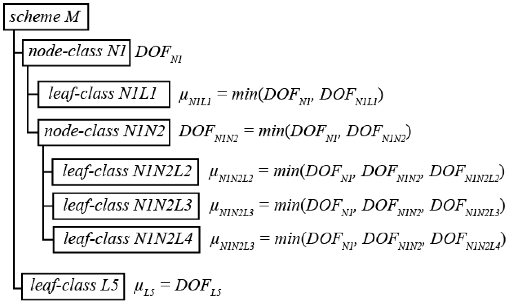
2.3. Defuzzification in Hierarchical Classification Schemes

In hierarchically organized classification schemes, fuzzy classified entities of L-classes may not fulfil the defuzzification criteria. Consequently they cannot be assigned to their BCR without any doubts, which means they cannot be defuzzified and therefore remain crisp-unclassified. Nevertheless, such entities could be doubtlessly assigned to one of their N-classes, especially if the class hierarchy describes the N-classes as physical commonalities of their L-classes. In such cases it is rather sensible to assign the entities of concern to that N-class whose DOF shows the maximum value: ${\mathsf{\mu }}_N=\text{max}(\overrightarrow{DOF})$ and fulfils the defuzzification criteria described above. For example the classes “Oak” and “Beech” may be possible subclasses of “Deciduous”. A fuzzy classified entity which neither fulfils the defuzzification criteria for “Oak” nor those for “Beech” but fully those for “Deciduous” can be doubtlessly crisp-assigned to “Deciduous”, instead of remaining unclassified. This process can be continued upwards in the hierarchy tree until the root-class of an entity is evaluated for defuzzification. In the example given, this could mean that if a clear decision is neither possible between “Oak” and “Beech” nor between “Deciduous” and “Coniferous”, the entity may still be classified as “Tree”, if “Tree” is the N-class of “Deciduous” and “Coniferous”. Otherwise it remains crisp-unclassified. The example demonstrates that the classification reliability can be increased at the cost of losing semantic details and vice versa.

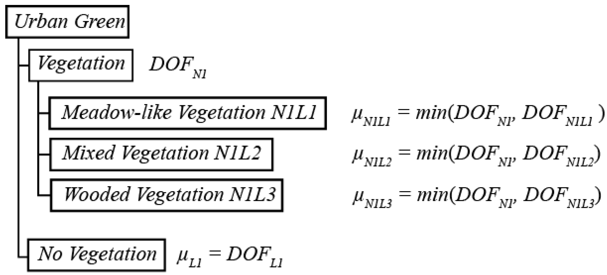
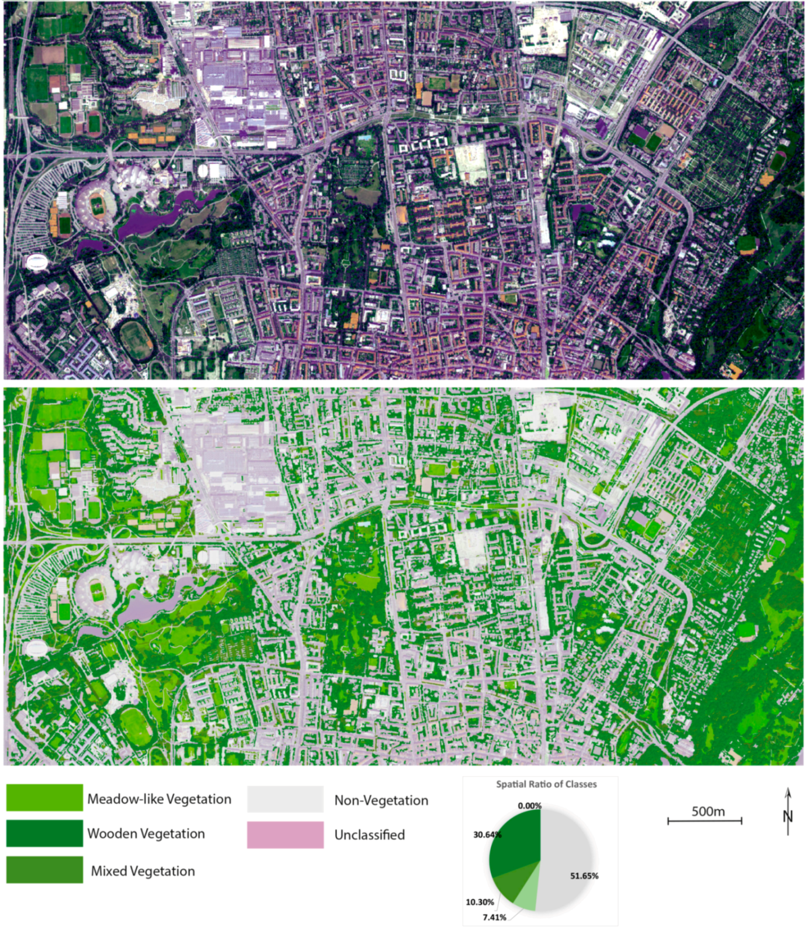
2.4. Example: Vegetation Map of Munich

This section demonstrates how the above mentioned defuzzification methods can be applied to achieve a least doubtable crisp classification result (defuzzification strategies), using an OBIA fuzzy classification result of urban green areas in Munich (Germany). The applied classification scheme is similar to that applied in [15]. It contains “Vegetation” and “Non-Vegetation” as N-classes. “Vegetation” is further sub-divided into three L-classes: “Wooden vegetation”, “Meadow-like vegetation” and “Mixed vegetation”. The class “No Vegetation” acts as the counterpart (the inverse) of “Vegetation” and is an L-class in the hierarchy (Figure 1 and Figure 2).

The scheme was applied on a subset of the WorldView-2 scene over Munich [22], captured on 10 July 2012 (coordinates: Left X = 688693; Right X = 694068.5; Upper Y = 5340051.5; Lower Y = 5337520.5, UTM Zone 32, Northern Hemisphere, Transverse Mercator, WGS 84), with the dimensions of 10,761 pixels × 5062 pixels. The scene was pan-sharpened using the principle components method proposed by Chavez [23], implemented in ERDAS Imagine 2013 software, using only those multi-spectral bands that cover the spectral range of the pan-channel, i.e., bands 2, 3, 4, 5, 6, and 7. The image was segmented using eCognition 9.1., in the manner described in Hofmann et al. [15]. The same software was used for the classification of the image and for developing the class hierarchy and fuzzy class descriptions. The brightness of each segment was calculated as the average DN value per object in bands 2, 3, 5, and 6. The segments generated were hierarchically classified according to the classification scheme described above (

Table 1. Classification scheme with class descriptions for detecting and differentiating urban vegetation.

Class	Properties	Membership Function	Function Values
			Lower Bound	Upper Bound
non-vegetation	NDVI		0.00	0.50
vegetation	NDVI		0.00	0.50
meadow-like vegetation	ratio NIR		0.12	0.17
	StdDev NIR		20.00	35.00
mixed vegetation	ratio NIR		0.35	0.75
	StdDev NIR		20.00	50.00
wooden vegetation	ratio NIR		0.30	0.50
	StdDev NIR		25.00	45.00

, Figure 2 and Figure 3). The “Vegetation” and “No Vegetation” classifications were based on the NDVI, calculated on a ‘per pixel’ basis and assigned to each segment as the mean of all pixel-values per segment. The N-class “Vegetation” is described by the mean NDVI per segment, as shown in Table 1. The L-classes “Wooded Vegetation”, “Meadow-like Vegetation” and “Mixed Vegetation” inherit this description, but are distinguished from each other by their relative brightness in band 6 (the so-called “red-edge” band [22]) when compared to the overall brightness of a segment (ratio red-edge) [15] and by the standard deviations of band-6-pixels within the segment of interest [15,24]. Figure 3 shows the initial results obtained by applying the rule set to the segmented image, together with the simplest defuzzification rule, (${\mathsf{\mu }}_0>0.0$). Segments fulfilling this condition are assigned to their BCR, regardless of their classification certainty, fuzziness or ambiguity.

3. Results

After classification, initially only L-classes are applied. The majority of the 46,534 segments (46,521 or 99.99%) had membership values of ${\mathsf{\mu }}_0>0.0$ to their BCR and 32,573 (70.02%) were assigned to their best and second-best class simultaneously, that is, with ${\mathsf{\mu }}_1>0.0$. Only three objects could not be classified at all, meaning they had no membership to any of the scheme’s classes (${\mathsf{\mu }}_0=0.0$). 38,277 objects had a membership to their BCR of ${\mathsf{\mu }}_0\ge 0.5$. The mean membership to the BCR was $\overline{{\mathsf{\mu }}_0}=0.78$, and $\overline{{\mathsf{\mu }}_1}=0.12$ for the second-best class (see Figure 4). The figure additionally shows that 831 objects are a member of all four classes, which is indicated by their ${\mathsf{\mu }}_3>0.0$. However, for the third- and fourth-best class (${\mathsf{\mu }}_2$ and ${\mathsf{\mu }}_3$) no object could achieve a membership of ${\mathsf{\mu }}_{2,3}>0.5$.

Table 2. Descriptive statistics of measures of uncertainty, fuzziness and ambiguity for the OBIA fuzzy classification result of the WV-2 scene of Munich.

	CSI	CSI*	CI	CI*	AIB	AISB	Fuzz1
Max	1.0000	1.0000	1.0000	1.4956	0.9931	3.7696	2.9912
Mean	0.6612	0.6542	0.3387	0.3457	0.2230	1.1917	0.4498
Min	0.0000	0.0000	0.0000	0.0000	0.0000	1.0000	0.0000
Standard Dev.	0.3294	0.3370	0.3293	0.3370	0.2636	0.3096	0.4264

depicts the descriptive statistics of the measures outlined in Section 2.2.3, which support the decision for the fuzzy classification’s defuzzification. Note: the maximum values for $C{I}^{*}$, $Fuz{z}_1$ and $A{I}_{SB}$ are below the possible maximum of $m=4$.

Both Figure 4 and Table 2 indicate that a variety of the fuzzy classified objects are not crisply assignable to their BCR without any doubts. Therefore, before defuzzification of these objects, their classification uncertainty, fuzziness and ambiguity should be evaluated. In case an object cannot be doubtlessly assigned to its BCR, a re-classification should be considered. Figure 5 and Appendix B depict the spatial distribution of the classification’s measures for uncertainty, fuzziness and ambiguity, calculated per object as described in Section 2.2.3.

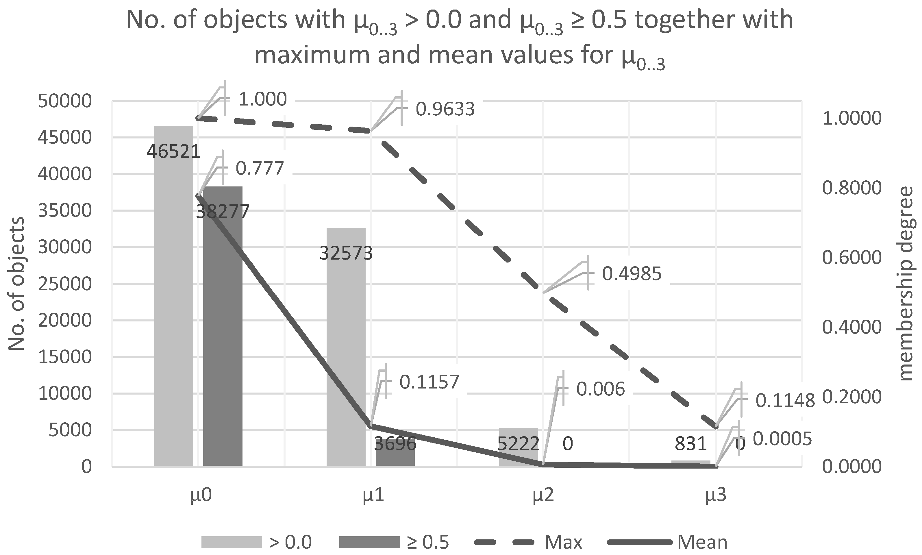
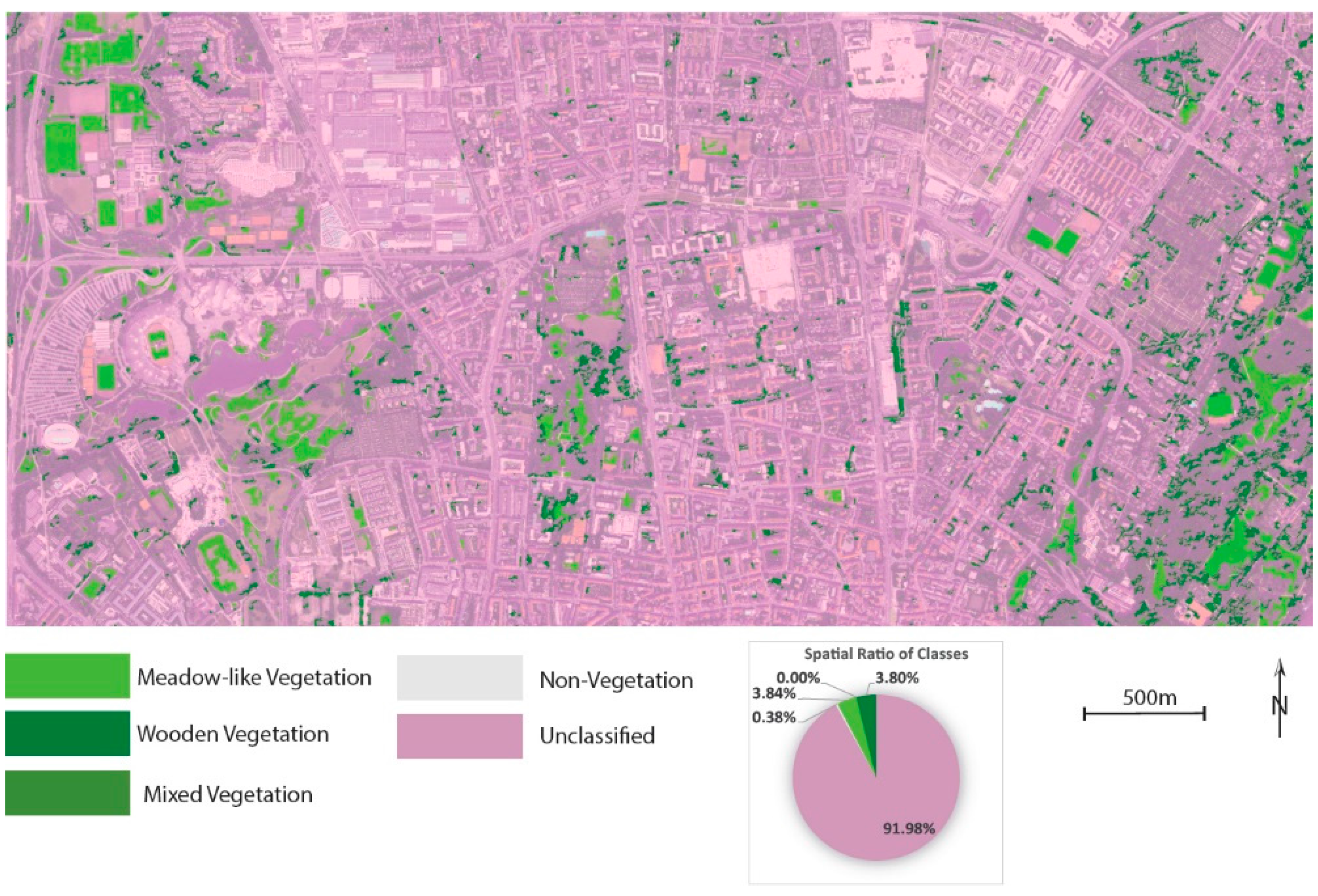
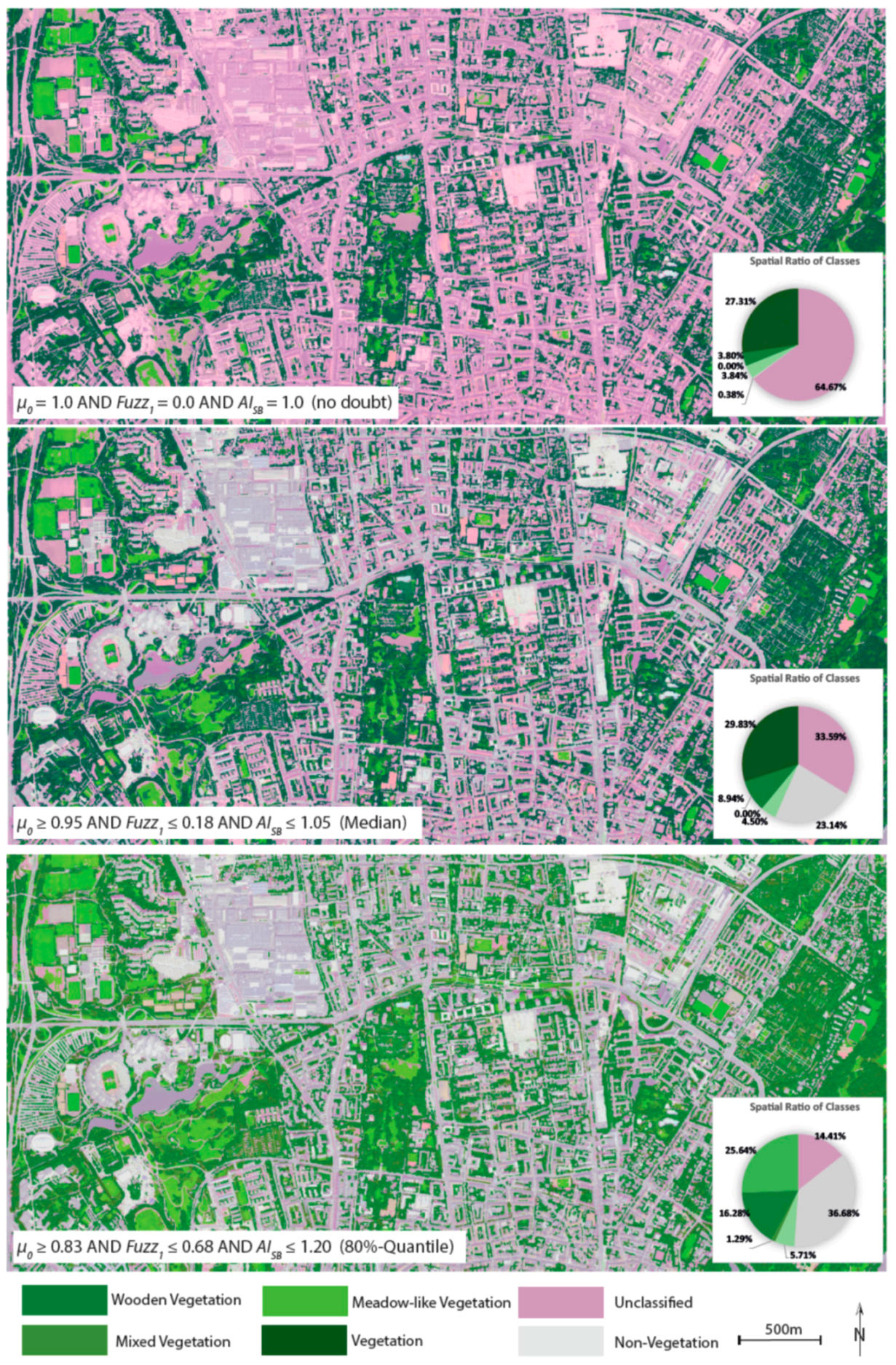
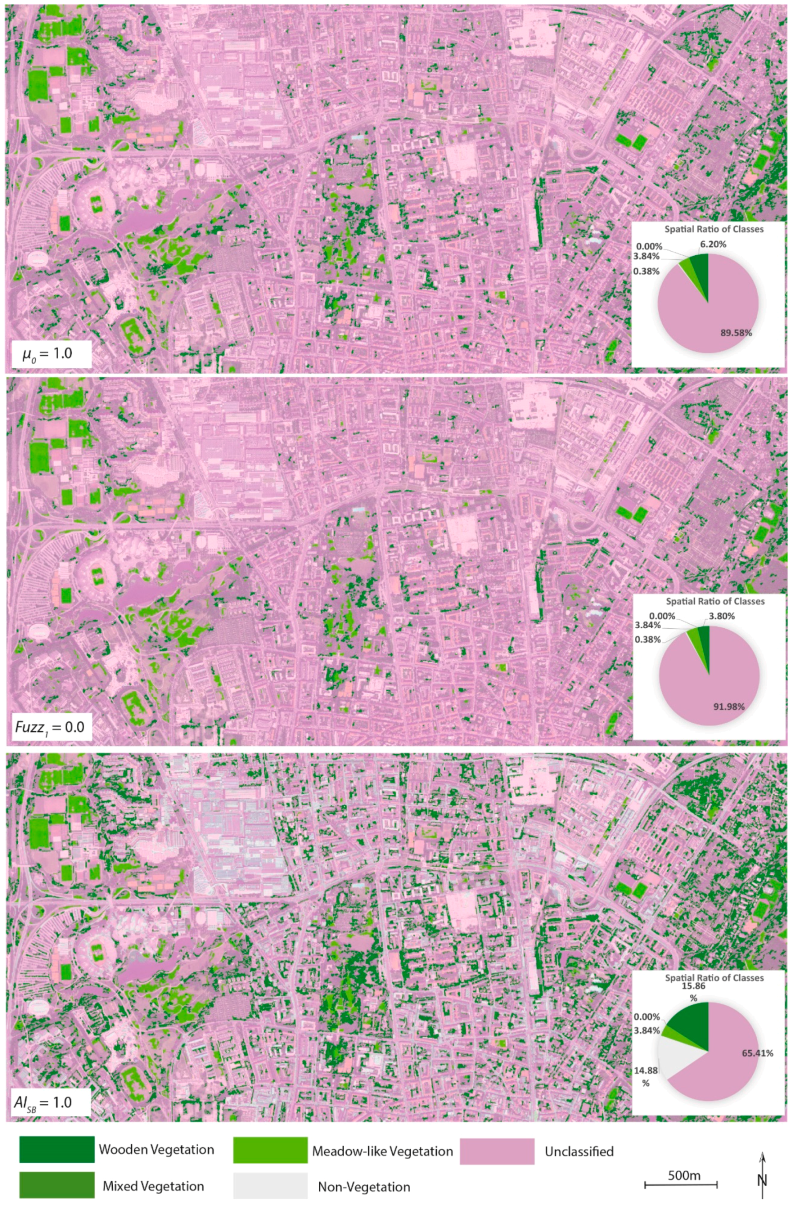
3.1. Defuzzification of Absolutely Doubtlessly Classified Objects

In the scene, 8247 objects (17.73%) have a membership degree of ${\mathsf{\mu }}_0\le 0.5$ to their best L-class. This result is considered as too uncertain for the respective objects to be assigned to their BCR (see Section 2.2.4). Vice versa, 3280 objects (7.05%) have a membership degree of ${\mathsf{\mu }}_0=1.0$ to their best L-class, and 2653 objects (5.70%), which cover 8.02% of the scene’s area, have a membership degree of ${\mathsf{\mu }}_0=1.0$ to their best L-class and of ${\mathsf{\mu }}_1=0.0$ to their second-best L-class. Accordingly, their fuzziness and ambiguity equals $Fuz{z}_1=0.0$ and $A{I}_{SB}=1.0$. Therefore these objects can be assigned to their BCR with absolutely no doubts (Figure 6).

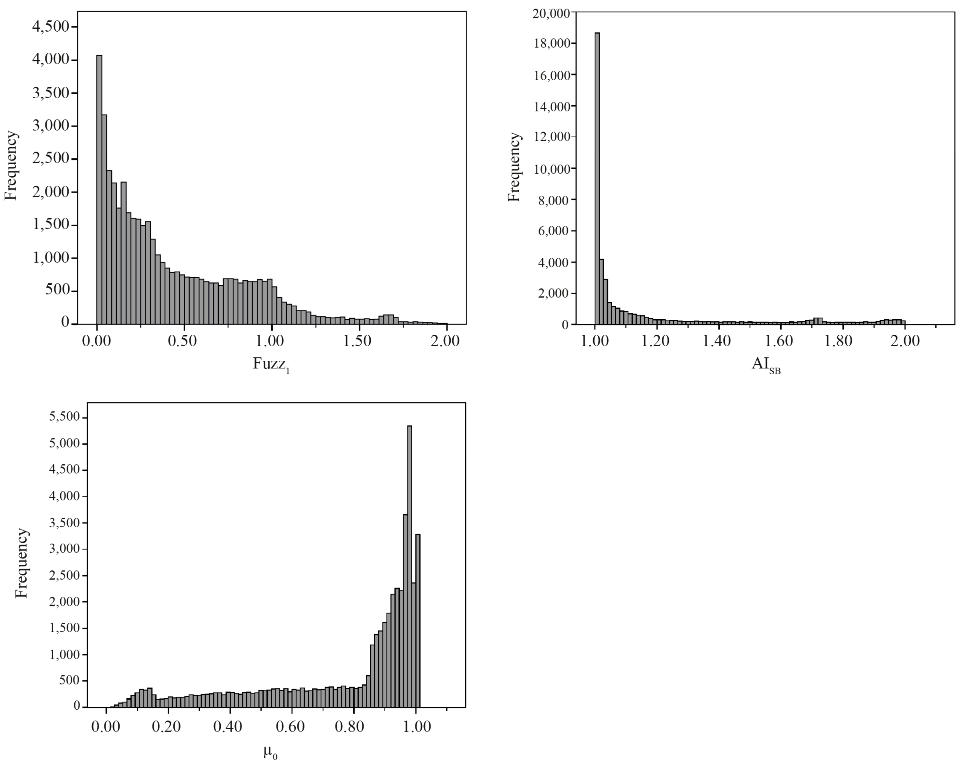
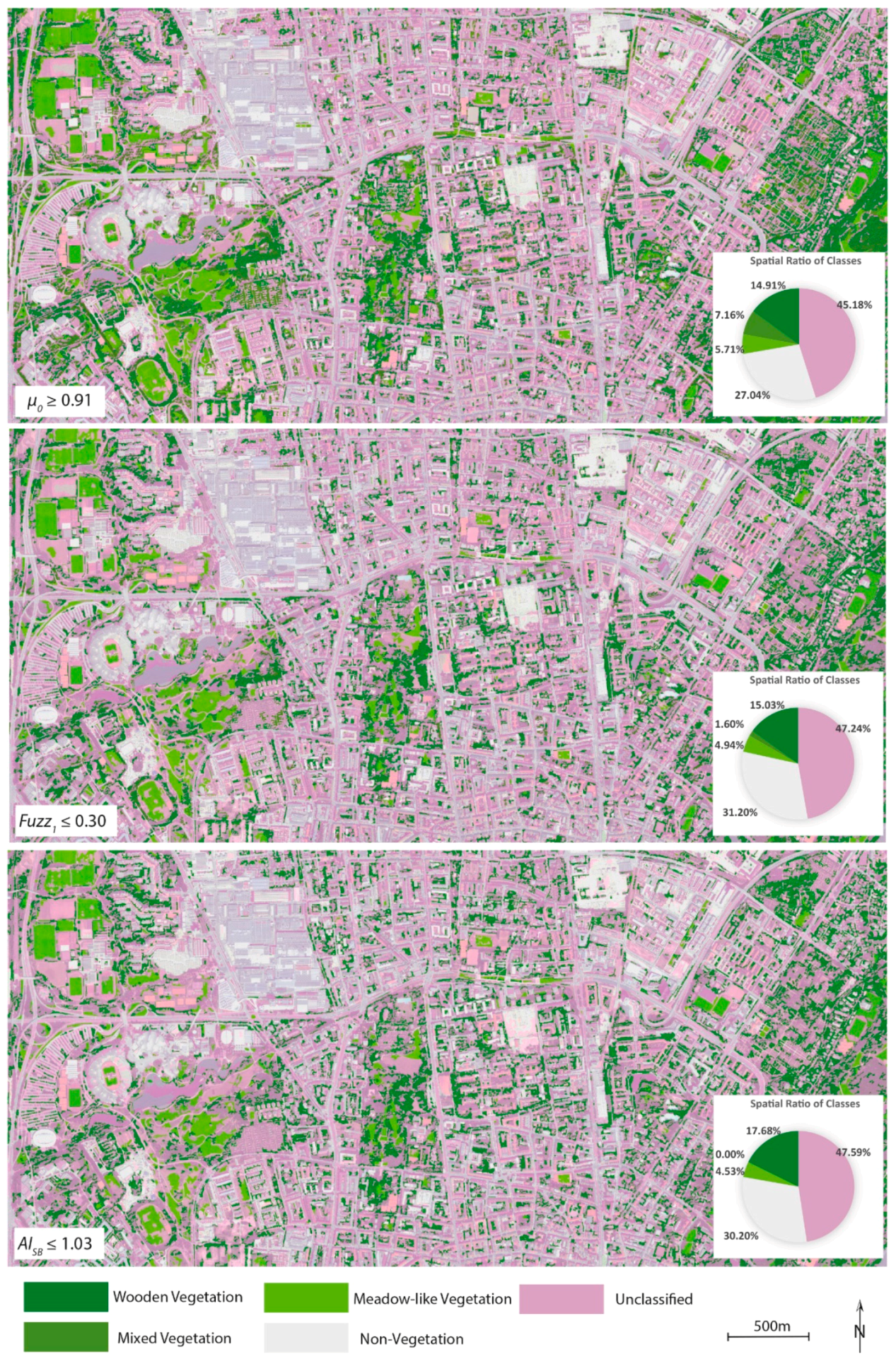
3.2. Defuzzification Based on Uncertainty, Fuzziness and Ambiguity

To defuzzify objects according to the measures outlined in Section 2.2.4, thresholds need to be set for each of them in order to define a defuzzification rule. However, the decision for defuzzification of a fuzzy classified object can be based either on a single criterion (uncertainty, fuzziness or ambiguity), or based on all of them simultaneously. The following consideration demonstrates what happens to the classification result if uncertainty, fuzziness and ambiguity are each regarded separately. That is, objects are defuzzified if they only fulfil a single defuzzification criterion. For example applying a threshold of ${\mathsf{\mu }}_0=1.0$ only, means objects which have a membership for their second-best class of ${\mathsf{\mu }}_1\ge 0.0$ are defuzzified. In the example, this yields 43,244 unclassified objects (92.95%), covering 89.58% of the scene’s area. Similarly, defuzzifying objects with $Fuz{z}_1=0.0$ leads to 43,868 unclassified objects (94.29%), yielding an area ratio of 91.98%. And if ambiguity is the only defuzzification criterion for all objects with $A{I}_{SB}=1.0$, 32,576 objects (70.02%) yielding 65.41% of the scene’s area are unclassified (see Figure 7).

However, applying defuzzification rules as demonstrated above leads to numerous crisp unclassified objects. Therefore some degree of uncertainty, fuzziness and ambiguity must be allowed in order to increase the ratio of classified area in the scene. To what extent this is acceptable must be decided on by the user. In any case, the thresholds should be set within the value ranges described in Section 2.2.4. Analysing quantiles for each measure helps to estimate the amount of crisp classified objects in a given scene resulting in thresholds for ${\mathsf{\mu }}_0$, ${\text{Fuzz}}_1$ and ${\text{AI}}_{\text{SB}}$ (see

Table 3. Percentiles of Fuzz₁, AI_SB and µ₀ of fuzzy classified objects of the WV-2 scene of Munich.

Percentile	Fuzz1	n with Fuzz1 ≤	AIB	n with AIB ≤	µ0	n with µ0 ≤
10	0.034	4653	1.000	13,951	0.036	4653
20	0.080	13,957	1.000	13,951	0.543	9304
30	0.144	13,958	1.000	13,958	0.725	13,958
40	0.217	18,610	1.013	18,610	0.862	18,610
50	0.303	23,262	1.028	23,262	0.901	23,262
60	0.443	27,915	1.063	27,915	0.936	27,915
70	0.616	32,567	1.148	32,567	0.964	32,567
80	0.813	37,219	1.370	37,219	0.977	37,220
90	1.012	41,872	1.747	41,872	0.991	41,872

and Figure 8).

Table 3 depicts the percentiles for the fuzzy classification result and the associated measures for uncertainty, fuzziness and ambiguity. As can be seen from Table 3 at least half of the number of all objects are crisp assigned to their BCR if the thresholds for their fuzzy classification measures are set to: ${\mathsf{\mu }}_0\ge 0.91$, $Fuz{z}_1\le 0.30$ and $A{I}_{SB}\le 1.03$ (Figure 9) and vice versa. Similarly to crisp assign for example, the best 80% of all objects, the parameters of ${\mathsf{\mu }}_0>0.54$, $Fuz{z}_1\le 0.81$ and $A{I}_{SB}\le 1.37$ must be fulfilled for each object; the remaining 20% of all objects are set to unclassified (Figure 10). In terms of assessing a classification’s quality, the percentiles can be interpreted as follows: in order to crisp assign a given percentage of objects to their BCR, according uncertainties, fuzziness and ambiguities (as displayed in Table 3) must be accepted by the user. Vice versa: the given classifier is only capable of classifying the number of objects as displayed in Table 3 if uncertainty, fuzziness and ambiguity per object are below the thresholds for each percentile.

Since each object in OBIA is in principle of individual size, the number of crisp assigned objects does not allow any conclusions about the covered area per percentile. However in the example given, all objects are of comparable size due to the unchanged initially applied Multi-Resolution Segmentation. Additionally, as can be seen in Figure 9 and Figure 10, although the quantity of classified objects is similar for each quantile-threshold, the quality of objects affected by the defuzzification rule is different, depending on the applied measurement criterion (certainty, fuzziness or ambiguity).

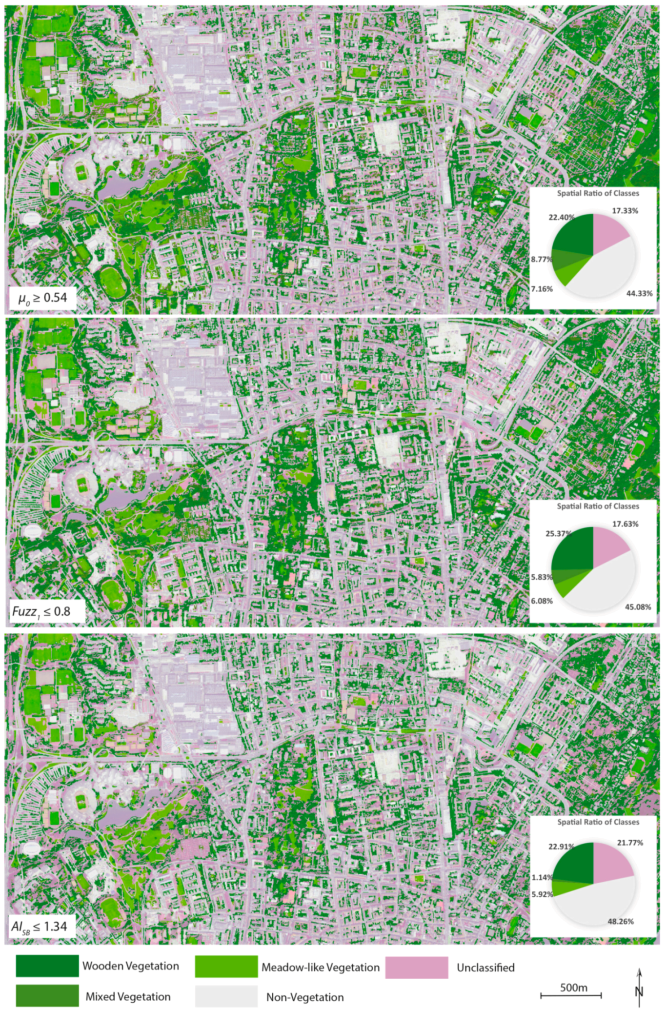
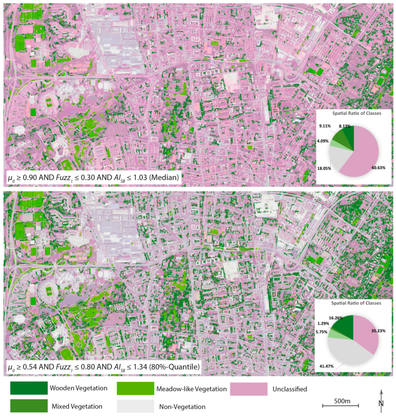
3.3. Defuzzification Based on Compound Criteria

Ideally, in order to defuzzify only the least doubtfully classified objects, each object should fulfil the criteria for all three measurements simultaneously, see Section 2.2.4 and Equation (11). When combining the three criteria, thresholds for each of the measures can be set differently depending on the user’s demands. Similar to the examples presented in the sub-section before, analysing the quantiles of a given scene for each measure is supportive in estimating the number of objects being defuzzified. However, results are different when thresholds for defuzzification are reduced and combined to a compound defuzzification rule with thresholds given by the percentiles for example, to: ${\mathsf{\mu }}_0\ge 0.90\wedge Fuz{z}_1\le 0.30\wedge A{I}_{SB}\le 1.03$ (median rule) and ${\mathsf{\mu }}_0\ge 0.54\wedge Fuz{z}_1\le 0.80\wedge A{I}_{SB}\le 1.34$ (80%-quantile rule).

Therefore, L-class objects must now fulfil the conditions for uncertainty (${\mathsf{\mu }}_0$), fuzziness ($Fuz{z}_1$) and ambiguity ($A{I}_{SB}$) simultaneously ($\wedge$-operator) to be defuzzified. A comparison of the results of the compound percentile rules with those of the single percentile rules (Figure 9, Figure 10 and Figure 11) reveals that the number of classified objects and area has clearly decreased (from approx. 53% to approx. 40% of the area for the median rules and from approx. 80% to approx. 65% of the area for the 80%-quantile rules). However, they now fulfil all the three criteria for uncertainty, fuzziness and ambiguity simultaneously (see Figure 11).

3.4. Re-Classification of Rejected L-Class Objects

When applying a hierarchical classification scheme, as is the case here, entities, also known as objects which cannot be defuzzified due to their uncertainty and/or fuzziness and/or ambiguity (rejected L-class objects being defuzzified as “unclassified”), might nevertheless sufficiently fulfil the classification criteria of one of their N-classes. For a crisp assignment to an entity’s N-class, the same defuzzification mechanisms can be applied as for its L-classes. In the present example “vegetation” acts as the N-class for “wooden vegetation”, “mixed vegetation” and “meadow-like vegetation”. Therefore, objects which cannot be clearly assigned to “wooden vegetation”, “mixed vegetation”, “meadow-like vegetation” or “non-vegetation”, could still be doubtless members of “vegetation” (or “non-vegetation”) instead of remaining unclassified. Accordingly, these objects can be re-classified, yielding a new membership value for the classes “non-vegetation” and “vegetation”. For the latter, new defuzzification thresholds can be determined and applied. In the example given, the measures of uncertainty, fuzziness and ambiguity did not change before re-classifying unclassified objects. After the re-classification of previously rejected objects, the percentiles for uncertainty, fuzziness and ambiguity changed, as displayed in

Table 4. Percentiles for ${\mathsf{\mu }}_0$, ${\text{Fuzz}}_1$ and ${\text{AI}}_{\text{SB}}$ measures after fuzzy re-classifying unclassified L-class objects to their according N-class.

Percentile	Fuzz1	AIB	µ0
10	0.000	1.000	0.669
20	0.000	1.000	0.830
30	0.048	1.012	0.888
40	0.101	1.026	0.923
50	0.178	1.047	0.955
60	0.306	1.083	0.975
70	0.446	1.126	0.988
80	0.680	1.205	1.000
90	1.323	1.494	1.000

. Naturally, the thresholds for the no-doubt rule did not change, but those for the median rule and the 80%-quantile rule changed to: ${\mathsf{\mu }}_0\ge 0.95\wedge Fuz{z}_1\le 0.18\wedge A{I}_{SB}\le 1.05$ (median rule) and ${\mathsf{\mu }}_0\ge 0.83\wedge Fuz{z}_1\le 0.68\wedge A{I}_{SB}\le 1.20$ (80%-quantile rule).

After re-classifying and defuzzifying unclassified objects according to the compound defuzzification rules, the class “vegetation” could be assigned and the number of unclassified objects reduced, as depicted in Figure 12. When applying the no-doubt defuzzification rule (${\mathsf{\mu }}_0=1.0\wedge Fuz{z}_1=0.0\wedge A{I}_{SB}=1.0$) the area ratio covered by unclassified objects reduced from almost 92% to approx. 65%, meaning that 35% of the area could now be doubtlessly assigned either to “vegetation”, “meadow-like vegetation”, “mixed vegetation”, “wooden vegetation” or “no vegetation”. Similarly, when applying the median-defuzzification rule the amount of unclassified area reduced from approx. 67% to approx. 34% when re-classified. Applying the 80%-quantile rule on the re-classified image objects reduced the amount of crisp unclassified objects to 9304 covering approx. 14% of the scene’s area. Only 1.29% of the scene’s area was re-classified as “vegetation”. The remaining objects are either a member of “no vegetation” or one of “vegetation’s” sub-classes (Figure 12).

4. Discussion

As was demonstrated in the present article, paying more attention to the classification’s uncertainty, fuzziness and ambiguity before starting the defuzzification of fuzzy classification results can increase the reliability of the final crisp classification result. As outlined in Section 2.2 and demonstrated in Section 3, classification uncertainty, fuzziness and ambiguity per entity can be measured in different ways by different measures. Some of these measures presented here and suggested in literature (see Section 2.2) are redundant. But as has been demonstrated, uncertainty (here measured by ${\mathsf{\mu }}_0$), fuzziness (here measured by $Fuz{z}_1$) and ambiguity (here measured by $A{I}_{SB}$) are the three major and independent aspects for evaluating a fuzzy classification’s reliability. However, as has been shown in Section 3 (see Figure 9, Figure 10, Figure 11 and Figure 12), evaluating only uncertainty, fuzziness or ambiguity alone is not enough to decide on a suitable defuzzification rule. Rather, it has been demonstrated that combining all three criteria to according defuzzification rules can maximize the reliability of the resulting crisp classification. Measuring a fuzzy classification’s uncertainty, fuzziness and ambiguity also supports the user in balancing between the area covered by crisp classified entities and their classification reliability, that is, between the crisp classification’s completeness and correctness. Section 3 demonstrated the relationship between achievable and intended reliability and achievable and intended area coverage. That is, for a given fuzzy classification rule set the user can a) evaluate its ability to assign entities to the desired classes in a reliable and spatially comprehensive way and b) to balance between area coverage (completeness) and the classification’s reliability (correctness). If the classes of a given scheme are organized hierarchically (fuzzy decision tree), completeness can be increased by reliably re-assigning doubtfully classified entities to their according parent classes (see Section 2.3 and Section 3.4). Therefore, objects that cannot be clearly assigned to one of the scheme’s leaf classes (L-classes), can be doubtlessly assigned to one of their node classes (N-classes) if the defuzzification criteria for this class are fulfilled. This way the classification coverage and reliability increase simultaneously, although the semantic level of detail decreases.

The results depicted in Figure 12, bottom show that if even a few objects could be doubtlessly re-assigned to their parent class (1.29% of the scene’s area were re-assigned to “vegetation”) the scene’s classification reliability increased: after re-assignment all crisp classified objects had a membership degree of at least ${\mathsf{\mu }}_0\ge 0.83$ instead of ${\mathsf{\mu }}_0\ge 0.54$ to their BCR, a fuzziness of $Fuz{z}_1\le 0.68$ instead of $Fuz{z}_1\le 0.80$ and an ambiguity of $A{I}_{SB}\le 1.20$ instead of $A{I}_{SB}\le 1.34$ (see Figure 11 and Figure 12).

When maximum reliability was implemented (no-doubt rule), the majority of non-vegetated areas remained unclassified, although almost all vegetation areas could be either assigned to one of the detailed vegetation sub-classes or to the general “vegetation“ class. This indicates that “non-vegetation” areas could not be absolutely doubtlessly identified in the image data using the developed class hierarchy and class descriptions. Therefore, in order to doubtlessly identify “non-vegetation” areas, the class definition should be revised.

Aside from the need for crisp final classification results, intermediate results may also need to be crisp for rather complex image analysis tasks, in order to stop or proceed processing, or to decide for a particular branch of further processing. For such complex tasks, adjusting the necessary reliability of the intermediate results can be performed through analysing their uncertainty, fuzziness and ambiguity, as presented herein. However, this has not been investigated yet.

In the context of Agent Based Image Analysis (ABIA), maximising the reliability of individual entities (aka image object agents), or the overall reliability of a fuzzy classification result could be defined as a goal for software agents, and therefore contribute to optimizing autonomously adapted rule sets or image objects [25].

5. Conclusions

Fuzzy classification rules for remote sensing data are designed by domain experts. They semantically describe the desired classes and their physical properties measureable by remote sensing sensors in a prototypical manner [26]. Thereby, the ideal representative of a given class fulfils all its criteria to 100% satisfaction. Measurements deviating from the ideal case lead to an explicit decrease of class membership, allowing experts to explicitly express their certainty or uncertainty about an entity’s membership to a particular class. For a particular entity (pixel or image segment) this means that if the measured values for its properties (DN values, shape properties, texture values etc.) do not fulfil the prototypical descriptions of a class to 100% satisfaction, the entity can still be a gradual member of this class. This allows entities to be a gradual member of several classes simultaneously, indicating that their class assignments are not 100% clear, that is, for a certain degree they are ambiguous and therefore unreliable. The latter can support rule set developers to rework the rule set design, for example to add or change rules for particular classes.

The advantages of fuzzy classification techniques in the context of remote sensing image analysis have been previously discussed in published literature [27,28]. The advantages for OBIA in particular have been outlined by Benz et al. [6] and Blaschke [29]. However, from a user’s perspective, fuzzy classification results are unwanted, since they are not or barely manageable [13]. Users actually expect crisp classification results that are as reliable as possible; whereas the individual user can decide to what degree he or she can accept uncertainty, fuzziness and ambiguity of the crisp classification results. As the example given demonstrates, the presented methods support the user in balancing between the crisp classification’s reliability and the amount of classified entities, that is, the area covered by (crisp and reliably) classified pixels or segments.

For hierarchical classification schemes with inheritance mechanisms as applied here, the classification’s reliability can be increased, when formerly unclassified entities are re-classified and fuzzy assigned to parent classes (N-classes) in the hierarchy. This way, although semantic precision decreases for these entities, the amount of classified entities can increase, while simultaneously the classification’s reliability is kept on a desired level. If unclassified entities cannot be assigned to one of their N-classes, adding sibling classes could be a solution.

Future investigations on defuzzification should also comprise defuzzification of intermediate fuzzy classification results and their reliability within rather complex analysis processes such as ABIA [25]. Especially in ABIA, quantified reliability, that is, a degree of reliability expressed by uncertainty, fuzziness and ambiguity, could be defined as a goal for agents to achieve in order to control autonomous adaptation processes. Analysis methods such as the Receiver-Operating-Characteristics (ROC) curve, as has been applied for segmentation optimisation by Drǎguţ et al. [30], should be further investigated in the context of fuzzy classification methods of remote sensing data.

References

1. Foody, G.M. Approaches for the production and evaluation of fuzzy land cover classifications from remotely-sensed data. Int. J. Remote Sens. 1996, 17, 1317–1340. [Google Scholar] [CrossRef]
2. Foody, G.M. Fuzzy modelling of vegetation from remotely sensed imagery. Ecol. Model. 1996, 85, 3–12. [Google Scholar] [CrossRef]
3. Zhang, J.; Foody, G.M. A fuzzy classification of sub-urban land cover from remotely sensed imagery. Int. J. Remote Sens. 1998, 19, 2721–2738. [Google Scholar] [CrossRef]
4. Siler, W.; Buckley, J.J. Fuzzy Expert Systems and Fuzzy Reasoning; Wiley: Hoboken, NJ, USA, 2005. [Google Scholar]
5. Yager, R.R. On the measure of fuzziness and negation part I: Membership in the unit interval. Int. J. Gen. Syst. 1979, 5, 221–229. [Google Scholar] [CrossRef]
6. Benz, U.C.; Hofmann, P.; Willhauck, G.; Lingenfelder, I.; Heynen, M. Multi-resolution, object-oriented fuzzy analysis of remote sensing data for GIS-ready information. ISPRS J. Photogramm. Remote Sens. 2004, 58, 239–258. [Google Scholar] [CrossRef]
7. Blaschke, T. Object based image analysis for remote sensing. ISPRS J. Photogramm. Remote Sens. 2010, 65, 2–16. [Google Scholar] [CrossRef]
8. Zadeh, L.A. Fuzzy sets. Inf. Control 1965, 8, 338–353. [Google Scholar] [CrossRef]
9. Yager, R.R. On ordered weighted averaging aggregation operators in multicriteria decisionmaking. IEEE Trans. Fuzzy Syst. Man Cybern. 1988, 18, 183–190. [Google Scholar] [CrossRef]
10. Shackelford, A.K.; Davis, C.H. A hierarchical fuzzy classification approach for high-resolution multispectral data over urban areas. IEEE Trans. Fuzzy Syst. Geosci. Remote Sens. 2003, 41, 1920–1932. [Google Scholar] [CrossRef]
11. Trimble. eCognition Developer 8.9 User Guide; Trimble: Munich, Germany, 2013. [Google Scholar]
12. Yager, R.R. Knowledge-based defuzzification. Fuzzy Sets Syst. 1996, 80, 177–185. [Google Scholar] [CrossRef]
13. Roychowdhury, S.; Pedrycz, W. A survey of defuzzification strategies. Int. J. Intell. Syst. 2001, 16, 679–695. [Google Scholar] [CrossRef]
14. Hatzichristos, T.; Potamias, J. Defuzzification operators for geographical data of nominal scale. In Proceedings of the 12th International Conference on Geoinformatics Geospatial Information Research: Bridging the Pacific and Atlantic, Gävle, Sweden, 7–9 June 2004.
15. Hofmann, P.; Strobl, J.; Nazarkulova, A. Mapping green spaces in Bishkek—How reliable can spatial analysis be? Remote Sens. 2011, 3, 1088–1103. [Google Scholar] [CrossRef]
16. Yager, R.R. On a measure of ambiguity. Int. J. Intell. Syst. 1995, 10, 1001–1019. [Google Scholar] [CrossRef]
17. Bhandari, D.; Pal, N.R.; Majumder, D.D. Measures of discrimination and ambiguity for fuzzy sets. In Proceedings of the IEEE International Conference on Fuzzy Systems, San Diego, CA, USA, 8–12 March 1992; pp. 145–152.
18. Burrough, P.A. Natural objects with indeterminate boundaries. In Geographic Objects with Indeterminate Boundaries; Burrough, P., Frank, A., Eds.; Taylor & Francis: Abingdon, UK, 1996; pp. 3–29. [Google Scholar]
19. Athelogou, M.; Schmidt, G.; Schäpe, A.; Baatz, M.; Binnig, G. Cognition network technology—A novel multimodal image analysis technique for automatic identification and quantification of biological image contents. In Imaging Cellular and Molecular Biological Functions; Springer: Berlin, Germany; Heidelberg, Germany, 2007; pp. 407–422. [Google Scholar]
20. De Luca, A.; Termini, S. A definition of a nonprobabilistic entropy in the setting of fuzzy sets theory. Inf. Control 1972, 20, 301–312. [Google Scholar] [CrossRef]
21. Pal, N.R.; Bezdek, J.C. Measuring fuzzy uncertainty. IEEE Trans. Fuzzy Syst. 1994, 2, 107–118. [Google Scholar] [CrossRef]
22. European Space Imaging (EUSI). Information Products Basic Imagery. 2013. Available online: http://www.euspaceimaging.com/static/images/files/pdf/BasicImagery-WVGA_web.pdf (accessed on 12 September 2013).
23. Chavez, P.S., Jr.; Sides, S.C.; Anderson, J.A. Comparison of three different methods to merge multiresolution and multispectral data: Landsat TM and SPOT panchromatic. Photogramm. Eng. Remote Sens. 1991, 57, 295–303. [Google Scholar]
24. Trimble. eCognition Developer 8.9 Reference Book; Trimble: Munich, Germany, 2013. [Google Scholar]
25. Hofmann, P.; Lettmayer, P.; Blaschke, T.; Belgiu, M.; Wegenkittl, S.; Graf, R.; Lampoltshammer, T.J.; Andrejchenko, V. Towards a framework for agent-based image analysis of remote-sensing data. Int. J. Image Data Fusion 2015, 6, 115–137. [Google Scholar] [CrossRef]
26. Belgiu, M.; Lampoltshammer, T.J.; Hofer, B. An extension of an ontology-based land cover designation approach for fuzzy rules. In GI_Forum 2013, Creating the GISociety: Conference Proceedings; Jekel, T., Car, A., Strobl, J., Griesebner, G., Eds.; Wichmann Herbert: Berlin, Germany, 2013; pp. 59–70. [Google Scholar]
27. Wang, F. Fuzzy supervised classification of remote sensing images. IEEE Trans. Geosci. Remote Sens. 1990, 28, 194–201. [Google Scholar] [CrossRef]
28. Mitra, S.; Pal, S.K. Fuzzy sets in pattern recognition and machine intelligence. Fuzzy Sets Syst. 2005, 156, 381–386. [Google Scholar] [CrossRef]
29. Blaschke, T.; Lang, S.; Lorup, E.; Strobl, J.; Zeil, P. Object-oriented image processing in an integrated GIS/remote sensing environment and perspectives for environmental applications. Environ. Inf. Plan. Politics Public 2000, 2, 555–570. [Google Scholar]
30. Drǎguţ, L.; Tiede, D.; Levick, S.R. ESP: A tool to estimate scale parameter for multiresolution image segmentation of remotely sensed data. Int. J. Geogr. Inf. Sci. 2010, 24, 859–871. [Google Scholar] [CrossRef]
Figure 1. Hierarchical classification scheme with the D O F s of the N- and L-classes. Only L-classes have a membership degree µ, expressed as the minimum of the L-class D O F L and of its N-classes’ D O F N .
Remotesensing 08 00467 g001
Figure 2. Class hierarchy of an Urban Green classification in a WorldView-2 scene of Munich.
Remotesensing 08 00467 g002
Figure 3. Top: Original image, standard deviation stretched (3.0%) R = WV-2 band 5; G = (WV-2 band 3 + WV-2 band 6)/2; B = WV-2 band 2. Bottom: Initial classification result for L-classes ( μ 0 > 0.0 ) superimposed over top image with 33% transparency.
Remotesensing 08 00467 g003
Figure 4. Descriptive statistics of µ0, µ1, µ2 and µ3 of “urban green” for the OBIA fuzzy classification result (L-classes) of the WV-2 scene of Munich.
Remotesensing 08 00467 g004
Figure 5. Objects’ membership degrees to the BCR ( μ 0 , upper), measured values for fuzziness (Fuzz1, lower left) and ambiguity (AISB, lower right) after segmentation and initial fuzzy classification (L-Classes) of WV-2 scene of Munich as depicted in Figure 3.
Remotesensing 08 00467 g005
Figure 6. Defuzzification of objects being a doubtless member of their BCR ( μ 0 = 1.0 and μ 1 = 0.0 ). of WV-2 scene of Munich.
Remotesensing 08 00467 g006
Figure 7. Crisp classification results after defuzzifying fuzzy classified objects of a WV-2 scene of Munich and their respective area coverage when applying the following single defuzzification rules: μ 0 = 1.0 , Fuzz 1 = 0.0 and AI SB = 1.0 .
Remotesensing 08 00467 g007
Figure 8. Histograms of Fuzz 1 , AI SB and μ 0 of fuzzy classified objects of the WV-2 scene of Munich.
Remotesensing 08 00467 g008
Figure 9. Crisp classification results after defuzzifying fuzzy classified objects of a WV-2 scene of Munich by applying the median for each measure as defuzzification rules ( μ 0 0.90 , F u z z 1 0.30 and A I S B 1.03 ) and their respective area coverage.
Remotesensing 08 00467 g009
Figure 10. Crisp classification results after defuzzifying fuzzy classified objects of a WV-2 scene of Munich by applying the 80%-quantile defuzzification rules ( μ 0 0.54 , F u z z 1 0.80 and A I S B 1.34 ) and their respective area coverage.
Remotesensing 08 00467 g010
Figure 11. Crisp classification results after defuzzifying fuzzy classified objects of a WV-2 scene of Munich and their respective area coverage by applying different compound thresholds as defuzzification rules.
Remotesensing 08 00467 g011
Figure 12. Crisp re-classifications of previously unclassified objects following defuzzification according to the defuzzification rules outlined in the text and indicated in each image.
Remotesensing 08 00467 g012