Abstract
All four chimpanzee sub-species populations are declining due to multiple factors including human-caused habitat loss. Effective conservation efforts are therefore needed to ensure their long-term survival. Habitat suitability models serve as useful tools for conservation planning by depicting relative environmental suitability in geographic space over time. Previous studies mapping chimpanzee habitat suitability have been limited to small regions or coarse spatial and temporal resolutions. Here, we used Random Forests regression to downscale a coarse resolution habitat suitability calibration dataset to estimate habitat suitability over the entire chimpanzee range at 30-m resolution. Our model predicted habitat suitability well with an r2 of 0.82 (±0.002) based on 50-fold cross validation where 75% of the data was used for model calibration and 25% for model testing; however, there was considerable variation in the predictive capability among the four sub-species modeled individually. We tested the influence of several variables derived from Landsat Enhanced Thematic Mapper Plus (ETM+) that included metrics of forest canopy and structure for four three-year time periods between 2000 and 2012. Elevation, Landsat ETM+ band 5 and Landsat derived canopy cover were the strongest predictors; highly suitable areas were associated with dense tree canopy cover for all but the Nigeria-Cameroon and Central Chimpanzee sub-species. Because the models were sensitive to such temporally based predictors, our results are the first to highlight the value of integrating continuously updated variables derived from satellite remote sensing into temporally dynamic habitat suitability models to support near real-time monitoring of habitat status and decision support systems.
1. Introduction
The dramatic decline in biodiversity has become so great that it is considered an important facet of global change in its own right [1]. Biodiversity loss has multiple causes, with habitat destruction via land-cover and land-use change as the predominant driver [2,3,4]. The majority of future land-use change will likely occur in tropical regions [5], which are home to almost half of all described species [6], including humans’ closest living relatives, the chimpanzee (Pan troglodytes). It has been estimated that more than 70% of chimpanzee tropical forest habitats are now threatened by infrastructure development and land use change [7]. All four chimpanzee sub-species (Western (P.t. versus), Nigeria-Cameroon (P.t. ellioti), Central (P.t. troglodytes), and Eastern (P.t. schweinfurthii)) have been classified as endangered on the International Union for the Conservation of Nature (IUCN) Red List. In fact, it has been estimated that their cumulative population has declined by more than 66% over the past 40 years [8] and there is a decreasing trend in population for all four sub-species [9,10,11,12]. Major threats to current populations include habitat loss from resource extraction activities and land conversion, hunting, disease and the illegal pet trade. Chimpanzees occupy a wide variety of forest and woodland habitats and serve as an umbrella species [13]; thus, protecting chimpanzee habitat could help conserve habitat for many other species.
The Open Standards for the Practice of Conservation (OSPC) provides a framework to guide the development and implementation of conservation projects [14]. OSPC is a collaborative and adaptive management process that strategically focuses conservation decisions on clearly defined objectives and prioritized threats and measures success in a manner that enables adaptation and learning over time. A key component outlined in the OSPC is an overall assessment of the viability or health of the conservation target and the establishment of a monitoring plan that requires indicators that are measurable, precise, consistent and sensitive [14]. Habitat suitability models (HSMs), also referred to as species distribution or ecological niche models, are useful tools that can fit easily within this framework. HSMs use statistical and machine learning techniques to find empirical relationships between observed species' occurrences and environmental descriptors, such as resource, biotic and climatic factors, to estimate conditions that are suitable for population viability [15], or to predict the likelihood of occurrence [16,17] in geographic space. Results from HSMs are most convincing when they are fit with both presence and absence data. However, due to the difficulty of acquiring ecologically meaningful absence data, HSMs are often constructed with so called ”presence only” data [18]. When models are fit with presence only data, the output can be interpreted as a relative measure of environmental suitability rather than the probability of presence [19,20] typically with a range between 0 (unsuitable) and 1 (highly suitable).
The use of HSMs to model and map chimpanzee habitat suitability is a recent endeavor and has been used to answer questions applicable to chimpanzee conservation and ecology. Vegetation layers derived from Landsat ETM+ data were used in [21] to model potential habitat suitability for chimpanzees in Western Tanzania at 90 m resolution. Landsat TM derived variables were used to generate habitat distribution maps for three time periods between 1986 and 2003 for a small area in Guinea-Bissau, within the range of P.t. verus, where a marked decrease in habitat area and connectivity was found [22]. Habitat suitability was mapped for the P.t. schweinfurthii range at 10 km resolution using climate, human impact and vegetation variables to aid in the delineation of areas for new population survey efforts [23]. HSMs were used for P.t. ellioti in Nigeria and Cameroon and P.t. troglodytes in Cameroon using climate, topographic, human population density and canopy cover variables at 1-km resolution to investigate the role of environmental variation in the genetic dissimilarity between the two sub-species and to assess potential future impacts of climate change on their habitat suitability [24]. The first range-wide study was performed by [25], who used climate, human impact and vegetation variables as model inputs to map habitat suitability for all four chimpanzee sub-species, and all African Great Apes, at 5-km resolution for both the 1990s and 2000s, and found a decrease in suitable habitat over time. Field researchers from several conservation organizations contributed data and were involved in the publication; thus, their results represent the most currently accepted and published state of chimpanzee habitat suitability across the field. We therefore rely on the results from Reference [25] for this study.
The objectives of this study are to map chimpanzee habitat suitability at 30-m resolution and provide information on changes in suitability through time to demonstrate that remotely sensed datasets that are updated on a continual basis can be used in near real-time conservation monitoring plans. Previous studies have attempted to determine the environmental variables that govern the observed distribution of chimpanzees at local, regional and range-wide scales. In this study, we determine which regularly updated remotely sensed variables are most useful indicators for effective and continuous monitoring of chimpanzee habitats. We utilized a modified version of habitat suitability modeling where, instead of using presence data to calibrate our model, we rescaled the coarse resolution habitat suitability map cited in Reference [25] to 30-m resolution using variables derived from remotely sensed datasets as input into a Random Forests regression model. Our results inform field monitoring efforts that support conservation planning and measure success as they portray finer scale habitat variation over several time periods.
2. Data and Methods
2.1. Study Area
The study area covers the ranges of the four chimpanzee sub-species that span central and western Sub-Saharan Africa over an approximately 2.3 × 10⁶ km2 area [26] (Figure 1), which represents approximately 7.5% of the African continental area. Chimpanzees occupy a wide variety of forest habitats across their range, including humid evergreen forests, mosaic woodlands, deciduous forest, and dry savanna woodlands [27]. Their habitats also cover a large elevation range, from sea-level in West Africa up to 2600 m in East Africa [26]. For our study, we used geographic range extents for each of the sub-species from the IUCN Red List. We buffered each range by 100 km to cover any suitable habitat that may fall outside the delineated range.
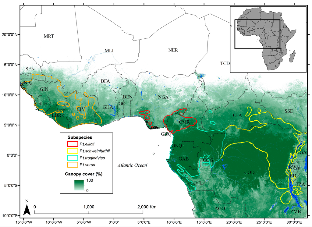
Figure 1.
Overview of study area with the International Union for the
Conservation of Nature (IUCN) Red List ranges of the four chimpanzee
sub-species overlaid on top of data showing percent canopy cover
from [28].
2.2. Habitat Data
Data on the spatial distribution of habitat suitability for most of the study area are from Reference [25], who used location data from the IUCN/Species Survival Commission A.P.E.S. (Ape Populations, Environments and Surveys) database (http://apes.eva.mpg.de), which serves as a central repository for all ape related survey data. Resulting estimates of habitat suitability were foundational for this study.
Logistic regression modelling was used in Reference [25] to develop HSMs. Logistic regression requires both a positive and negative outcome. In this case, known chimpanzee locations were used as the positive outcome and the negative outcome was composed of “pseudo-absences”. Pseudo-absences were selected based on the output from MaxEnt, a software package widely used to generate habitat suitability models where presence only data are available [29]. Grid-cells with low predicted suitability from the MaxEnt model were more likely to be used as the negative outcome in the logistic regression models. Predictor variables used in Reference [25] included bioclimatic variables from the WorldClim dataset, forest cover products derived from the Moderate Resolution Imaging Spectrometer (MODIS) and the Advanced Very High Resolution Radiometer (AVHRR) sensors, human population density, proximity to roads and proximity to navigable rivers.
Location data covering the dry forests and miombo woodlands of western Tanzania were not included in the APES database; therefore these important chimpanzee habitats were not reflected in the output from Reference [25]. In order to include these habitats in our model, we incorporated a habitat suitability model created by the authors of [21] specifically for this region based on nest locations (Figure 2B). Mahalanobis distance was used to relate chimpanzee location data, collected as part of biodiversity surveys conducted by the authors of [30], to three environmental predictors: distance to the nearest forest patch, distance to steep slopes (i.e., slopes greater than 20°) and elevation [30]. In the context of habitat suitability modeling, the Mahalanobis distance is the squared difference (in feature space) between a vector of values for the environmental predictors at un-sampled locations and the vector containing the mean values for the same predictors at sampled locations [31]. Mahalanobis distances are approximately distributed as Chi-square with n degrees of freedom where n is the number predictor variables, therefore a location that has a vector identical to the mean vector will have a typicality of 1.0 while larger distances will approach a typicality of 0 [32]. In order for the prediction from this model to be on the same scale as [25], Mahalanobis distances were converted to typicality probabilities by assuming a Chi-square distribution with three degrees of freedom. The suitability map was then coarsened from its native 90-m resolution to approximately 5-km resolution and combined with the 2000s prediction produced by Reference [25].
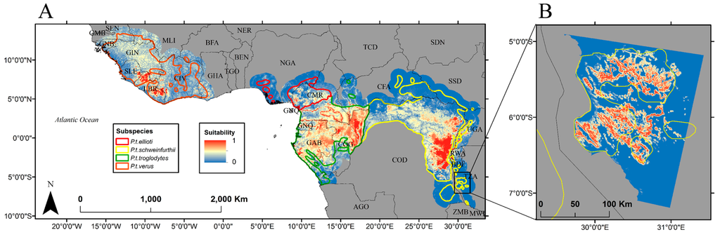
Figure 2.
(A) Habitat suitability data used for Random Forest
calibration [25] and (B) habitat suitability data for the miombo
woodlands of western Tanzania [21].
2.3. Satellite Data
Spectral reflectance, forest structure and forest loss data were from a recent processing and synthesis of the Landsat ETM+ data archive performed by the authors of [28]. This dataset consists of global annual composites of percent canopy cover, canopy height, and top of canopy reflectance for Landsat ETM+ bands 3, 4, 5 and 7, as well as annual data of forest loss from 2000 to 2012. The global products are in a geographic coordinate system and were disaggregated into 10° × 10° tiles with a resolution of 0.000278 decimal degrees (~30 m). To reduce the effects of noise and to fill data gaps due to persistent cloud cover, we divided the annual composites into four time periods by applying a three year median to the canopy cover, canopy height, and spectral band layers, resulting in datasets representing 2000–2003, 2004–2006, 2007–2009, and 2010–2012 time periods. The method for generating Landsat based canopy cover and forest loss data can be found in Reference [28], however the canopy height data were not included as part of the initial data release. Global tree height maps were generated on an annual time scale using a regression tree model that related height measurements from the Geoscience Laser Altimeter System (GLAS), part of the ICESat satellite mission, to Landsat time-series metrics. These height maps were used in Reference [33] to estimate carbon emissions from natural and managed forests; model error was quantified using a random 90% subset of the available GLAS data to train the model while the remaining 10% was used for testing model performance. Root mean square error and mean absolute error for the tropics was 8.1 m and 5.9 m, respectively. For additional information on the method used to generate the tree height maps from Landsat data, see Reference [34].
Topographic data for the study region were from the Shuttle Radar Topography Mission (SRTM) 3 arc-second resolution dataset and locations of rivers were from the SRTM Waterbodies Dataset (SWBD). The SWBD was created as a by-product of the finished SRTM DEM and includes water bodies detectable at approximately 30-m resolution at the time of the SRTM shuttle flight, circa February 2000 [35]. The SWBD is distributed in vector format, which we rasterized to ~30-m resolution to match the resolution of the Hansen et al. 2013 [28] dataset. We also resampled the elevation and slope layers to ~30 m to match the resolution of the dataset in Reference [28].
Derivation of Predictor Variables and Calibration Data
A full list of predictor variables used to construct the habitat suitability models is shown in Table 1. We identified the set of predictor variables based on the variables used to generate the HSMs in Reference [25] and variables used in other studies on chimpanzee habitat suitability. Canopy cover and canopy height were included in the set of predictor variables because measurements of forest structure (e.g., percent canopy cover) were found to be important in the determination of chimpanzee habitat suitability in several previous studies [23,24,25]. Spectral metrics, namely NDVI, were found to be an important predictor in Reference [22], which they argued served as a proxy for ecosystem functioning. We chose to include all Landsat ETM+ bands and band derivatives from the dataset in Reference [28] for this reason and because several studies have found an association between spectral data and forest structure metrics [36,37,38].

Table 1.
List of predictor variables used as input to Random Forest regression models.
Distance to the nearest forest patch was used as a predictor variable both in the habitat suitability models for Western Tanzania [21] and in Reference [22], and was therefore included in the set of predictor variables. In this study, we defined forest as 40% canopy cover with a minimum patch size of 0.5 ha, which is a combination of definitions used by the United Nations Environment Programme (UNEP) and Food and Agriculture Organization (FAO) for closed forests [39,40]. We applied a threshold of 40% or greater to the canopy cover layers and removed patches smaller than 5 Landsat pixels or approximately 0.5 ha. We used these layers to calculate the minimum per pixel distance to the nearest forest patch for all four time periods.
Human impacts on chimpanzee habitat were found to be important in References [24,25], and Reference [23] that used some form of gridded human population as a predictor variable. Deforestation and forest fragmentation are the direct result of human activity and are known to adversely affect biodiversity [41]. In this study, we used forest loss and fragmentation metrics as proxies for human impact on chimpanzee habitat. We created forest edge layers for each time period by calculating the per pixel distance from the interior of each forest patch to the nearest forest edge. In addition, we calculated the proportion of forest edge within a buffer of 1 km and 25 km for each pixel. We chose a buffer of 1 km to capture the influence of local scale fragmentation while the 25 km diameter represents the upper limit of a chimpanzee’s home range [42,43,44].
We used the forest loss data from Reference [28] to create four binary loss/no-loss layers for 2000–2003, 2004–2007, 2008–2009, and 2010–2012 time periods. To clean the data, we removed pixels that were labeled as forest-loss in non-forest pixels and used the same minimum size to define forest patches (i.e., 0.5 ha). We used these layers to calculate the per-pixel distance to the nearest forest loss patch and the proportion of loss in 1 km and 25 km in diameter, respectively.
We used topographic information including elevation, slope and distance to steep slopes as predictor variables in our model because previous studies have found they factor into the prediction of chimpanzee habitat suitability. Chimpanzee nests were generally found to be absent in forests and woodlands in elevations greater than approximately 1900 m [21,23]. In addition, chimpanzees have been found to potentially prefer to nest on steep slopes, with a grade greater than 20°. Slope was found to be a prominent factor in the prediction of habitat suitability in Reference [24], particularly for the P.t. ellioti sub-species. Finally, we used the rasterized SWBD dataset to calculate the per pixel distance to rivers because the authors of [25] found proximity to rivers to be a significant predictor of habitat suitability in all of their models. We decided to use the SWBD dataset to map the range-wide river network rather than the Digital Chart of the World data used in Reference [25], as it is a more current depiction of the river network.
In order to match the spatial resolution of the calibration dataset, all predictor variables for the 2000–2003 time period were resampled from 30 m to 5 km by averaging all 30 m pixels within a 5 km grid-cell. Values for the habitat suitability layer and predictor layers were extracted for each of the four sub-species ranges resulting in 18,000, 71,500, 45,000, and 48,000 samples (i.e., 5-km grid-cells) for P.t. ellioti, P.t. schweinfurthii, P.t. troglodtyes and P.t. verus, respectively. We generated fifty boot-strapped training and testing datasets for each sub-species by randomly sampling 75% of each dataset for model calibration and 25% for model validation. We created an additional fifty training and testing datasets that represented the entire chimpanzee range by combining training and testing datasets from each sub-species. We then predicted habitat suitability from the range-wide, 5-km resolution calibration map using a suite of remotely sensed derived metrics (Table 1).
2.4. Habitat Suitability Estimation
We used Random Forests regression to estimate range-wide chimpanzee habitat suitability with the Sci-kit Learn module in the python software environment [45]. Random Forests is an ensemble technique in the Classification and Regression Trees (CART) family of machine learning methods [46]. Random Forests works by constructing several regression trees based on bootstrapped samples of the input dataset and each node is split using the best from a random subset of predictors and each tree is grown to full size. Overfitting in Random Forests is avoided by averaging the predictions produced by individual trees. Random Forests have the attractive properties of being insensitive to non-normally distributed variables, non-linear relationships, and co-linear predictor variables [47]. In addition, only two primary parameters are required for Random Forest models; the number of trees constructed in each forest and the number of variables to consider at each node split.
We calibrated Random Forests regression models using satellite data from 2000–2003 to have a close temporal match with Reference [25]. The climate, demographic and topographic variable data used in Reference [25] are not updated regularly and could presumably be used to predict habitat suitability over a fairly wide temporal range. Canopy cover metrics, on the other hand, were from AVHRR and MODIS continuous field estimates representing forest in the first few years of the 2000 decade.
While the authors of [25] created a separate model for each sub-species, we investigated if a general, range-wide model could reasonably predict habitat suitability for each of the sub-species. An initial Random Forests regression model was constructed for each bootstrapped training sample for each sub-species as well as a general, range-wide model from the pooled sub-species data. Predictions were made from each model on the test data, and Root Mean Square Error (RMSE) was computed for each bootstrapped sample. A preliminary analysis indicated that using a range-wide model to predict suitability for each of the sub-species ranges did not result in a substantial increase in error for any of the sub-species (Figure 3). We therefore focused on the development of a general, range-wide model for the remainder of this manuscript.
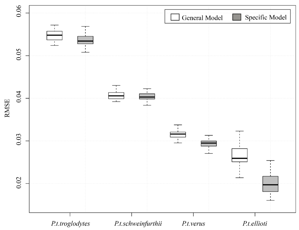
Figure 3.
Boxplots of 50-fold cross-validated RMSE of a general, range-wide model (white) and four models trained on data for each of the individual sub-species (grey).
2.4.1. Selection of Predictor Variables
To create the most parsimonious model possible, we first removed highly correlated variables in addition to the variables that contributed little to the predictive capability of the model. We created a correlation matrix for all predictor variables to determine the coefficient of determination for each combination of variables. For each pair of highly correlated variables (r2 > 0.9), we calculated the coefficient of determination between each variable and habitat suitability and retained the predictor variables with the highest coefficient of determination. We found canopy height and percent canopy cover to have a correlation coefficient greater than 0.9; however, we decided to retain both variables because of their recognizable ecological importance to chimpanzee habitat. Next, we used recursive feature elimination to remove variables that had little influence on the model’s predictive power. Recursive feature elimination operates by first ranking all variables by a measure of importance. Here, we ranked variables by the mean increase in RMSE when the values for a particular variable were randomly permuted [48]. The variable that resulted in the smallest increase in RMSE was dropped and a new model was created, and new ranks were then calculated for each variable. We continued this process until RMSE reached a minimum [49]. The lowest RMSE occurred when a subset of 12 variables was used to construct Random Forest models. Mean RMSE for models created using a subset of variables (0.041 ± 0.002) was slightly lower, but not significantly different than the mean RMSE (0.042 ± 0.003) from models created using the full set of variables.
2.5. Habitat Suitability Prediction
We used all samples from the calibration dataset to train the final Random Forests model of habitat suitability. We found that out of bag (i.e., the sample withheld during the construction of trees) error stabilized when a forest was created with 250 trees and 7 of the variables considered at each node split. The final Random Forest model was used to create range-wide habitat suitability maps for the 2000–2003, 2004–2006, 2007–2009 and 2010–2012 time periods at the 30-m Landsat pixel scale.
3. Results
We found similar spatial patterns of habitat suitability between the calibration data (Figure 4A) and the predictions from our model (Figure 4B). Moreover, we were able to model chimpanzee habitat suitability reasonably well compared to the calibration data, explaining 82% (±0.2%) of the variance for the entire chimpanzee range (Table 2). However, there was considerable variation in the model’s predictive capability among the four sub-species. Our model was able to explain 35% (±1.95%), 89% (±0.18%), 66% (±0.47%), and 73% (±0.44%) of the variance for P.t. ellioti, P.t. schweinfurthii, P.t. troglodytes, and P.t. verus, respectively (Table 2). Compared to the calibration data, our model tended to underestimate habitat suitability (Figure 5A,B). In general, areas where suitability was underestimated occurred at low elevations with sparse canopy cover, while the opposite was true for overestimated areas. Linear error patterns could be seen within the range of P.t. troglodtyes (Figure 5A), which resulted from a spatial mismatch of rivers between our study and Reference [25] due to differing river network datasets.
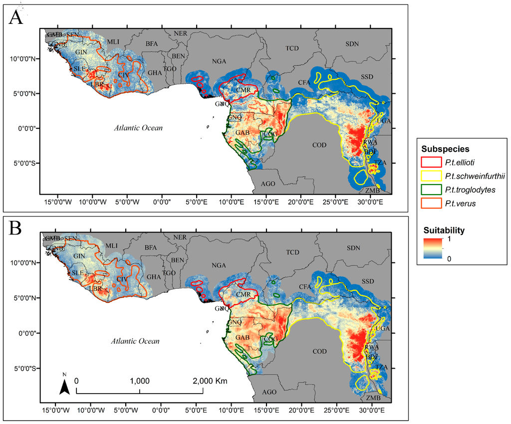
Figure 4.
Spatial distribution of suitability values for 5-km resolution map (A), and Random Forests prediction at 30-m resolution (B).
Table 2.
Cross-validated mean correlation coefficients with standard errors (N = 50 cross validations) reported for the entire chimpanzee range, as well as for each sub-species.
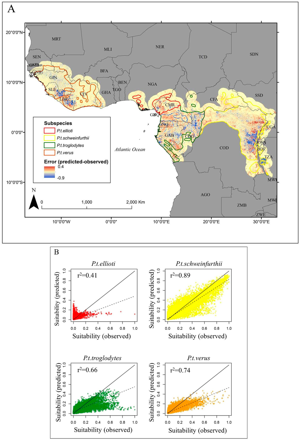
Figure 5.
Spatial distribution of differences between the 5-km resolution map used for model calibration and the 30-m map after coarsening to 5-km resolution (A), distribution of suitability values of 5-km calibration map (x-axis) and coarsened 30-m map (y-axis) for each sub-species (B). The one-to-one line is shown in solid black and results of regressing values from the coarsened 30-m map onto values from the 5-km map for each sub-species are shown by the dashed black line.
Elevation, Landsat ETM+ band 5 and Landsat derived canopy cover were the strongest predictor variables in our model (Figure 6). A significant association between habitat suitability and bioclimatic variables was found in the suitability models for all four sub-species in Reference [25]. The bioclimatic variables used in Reference [25] were taken from the WorldClim set of global climate layers, which were created by interpolating weather station data using latitude, longitude and elevation as independent variables [50]. It is therefore probable that elevation acted as a proxy for suitable climate conditions in our model. Shortwave infrared reflectance is highly correlated with forest/non-forest, where forests have lower reflectance due to absorption properties of live vegetation and light extinguishing effects of tall forest canopies. The value of band 5 in discriminating Congo Basin forest from non-forest was illustrated in Reference [51]. Trees in the CART family have been shown to exhibit a bias toward variables that have many cut-points (i.e., variables with many unique values) [48]. Band 5 is tightly correlated with canopy cover (r2 = 0.83) and canopy height (r2 = 0.82) in the calibration data. Canopy cover values were all integers between 0 and 100, while canopy height values were all integers between 0 and 23. On the other hand, band 5 values were continuous on the interval 0 to 0.7, which provided the algorithm with many more possible cut-points relative to canopy cover and canopy height. We believe it may therefore likely be driving the model as a surrogate for forest structure.
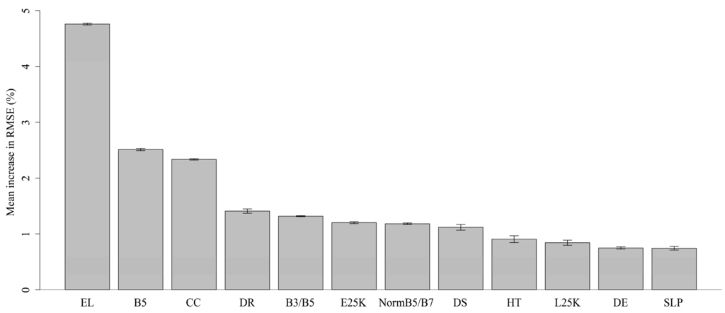
Figure 6.
Relative importance of 12 variables selected for final Random Forest model after recursive feature elimination. Confidence intervals (95%) were calculated using bootstrap sampling (N = 50). Variable importance was measured by the mean increase in RMSE % when values for a variable were randomly permuted.
4. Discussion
This study represents the first attempt to map temporal dynamics of range-wide chimpanzee habitat suitability at a finer spatial scale. Our model demonstrated sensitivity to environmental change, which is a key feature for monitoring applications. The area depicted in Figure 7 is situated in the Republic of Congo, which historically has not experienced any substantial human disturbance but recently has seen the most rapid increase in the establishment of logging roads among all Central African nations [51]. Our model was able to detect the fine-scale changes in habitat suitability due to human activities in the area (Figure 7B–E), whereas the coarse scale model was unable to resolve any fine-scale variation (Figure 7F). These results highlight the value of integrating continuously updated variables derived from satellite remote sensing into habitat suitability models for near real-time monitoring and decision support. The Landsat suite of satellites has provided the longest continuing record of standardized data of Earth’s land cover at 30-m resolution; metrics derived from these data will be crucial for the development of standardized habitat suitability models that can be repeated and integrated into long-term monitoring plans.
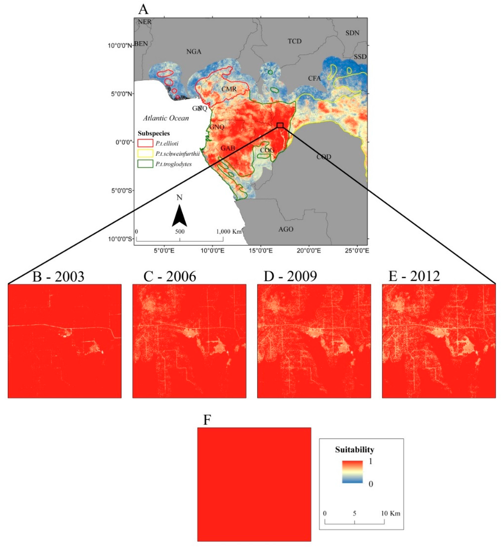
Figure 7.
Suitability values predicted by a Random Forests model for
Central Africa (A), an area experiencing selective logging circa
2003 (B), circa 2006 (C), circa 2009 (D), circa 2012 (E) and the area
as depicted in the 5-km resolution calibration data (F).
Previous studies have reported successful efforts to model chimpanzee habitat suitability, including the two sources from which our model was calibrated. Direct comparison between studies is difficult because, so far, there are only a few published studies and they generally do not have overlapping study areas or represent habitat at substantially different spatial scales. All studies except for Reference [30] utilized the MaxEnt software to generate their models, which reports model accuracy based on the Area Under the Curve of the Receiver Operating Characteristic (AUC). AUC characterizes the performance of a model at all possible thresholds by a single number that represents the probability that a known presence location will be ranked higher than a random background location [29]. Typical values for AUC are between 1.0–0.5 where a value of 1.0 represents a perfect fit while 0.5 indicates the model is no better than a random expectation [29]. The first study to use Landsat data to model chimpanzee habitat suitability was Reference [22] and reported an average AUC value greater than 0.9 indicating a good model fit. In addition, they were also able to detect changes in habitat suitability between two time periods. While their study area was much smaller than ours, a 2700 km2 region in Guinea-Bissau, it lends support to the approach of using Landsat data to detect changes in chimpanzee habitat suitability. Similar AUC values were reported in Reference [25], the primary calibration data source for our model, which ranged from 0.86 to 0.93. The authors of [25] were able to compare their habitat suitability model for P.t. schweinfurthii to the results from Reference [23] and found large differences in the spatial distribution of habitat suitability for this sub-species. However, the maximum AUC reported in Reference [23] was 0.67, which suggests the results from Reference [25] are a better representation of habitat for this sub-species. Due to a lack of calibration data, important miombo woodland habitat in Western Tanzania was predicted as unsuitable in Reference [25], which is the reason we included model output from [30] in our calibration data. While the authors of [30] did not provide AUC values for their model, they did assess model predictions with a 25% excluded portion of the nest locations that was not used to create the Mahalanobis distance model and an independent dataset from historical surveys. They found 92% of nests that were not used in model calibration and 84% of nests from historical surveys fell into the moderate to high suitability range. This indicates that the model was able to predict suitable nesting sites, but unfortunately does not provide any information about the model’s commission error.
While our model performed well across the chimpanzee range, it did show variation in its predictive capability. Compared to the calibration data, our model underestimated regions of high suitability in the P.t. ellioti and P.t. troglodytes ranges, which is likely due to missing predictor variables. We found dense canopy cover to be an important predictor of habitat suitability in our model, however; the authors of [25] did not find canopy cover to be a significant predictor variable in their models for these two sub-species. Both of these sub-species are found in central Africa, which is thought to be the last bastion of contiguous high quality chimpanzee habitat. While these large tracts of undisturbed forest are likely suitable places for chimpanzees to live, recent research has found a catastrophic decline in populations due to intense bush-meat hunting and disease [52]. High value tree species are selectively logged in the region, which leaves forests largely intact; however, the creation of logging roads opens up previously isolated forests, increasing the frequency of human contact and allowing easier access for hunters [52,53]. An absence of chimpanzees in these intact forests is likely the reason why habitat suitability is low in these areas and incorporating information on the proximity to logging roads and camps would benefit model accuracy.
It is important to note that inaccuracies in our model could also arise from errors in the input datasets to our model as well as errors in the datasets used to calibrate our model. Tree canopy cover was an important predictor variable in our model and was derived from Landsat ETM+ spectral data [28]. Canopy cover estimates from satellite data can be influenced by the composition of understory vegetation, satellite signal saturation and phenological noise [54,55]. Moreover, tree canopy cover from Reference [28] does not discriminate between forest types which could lead to predicting suitable habitat in intensely managed forests. Habitat suitability models in Reference [25] were generated using bioclimatic variables from the WorldClim dataset and considerable uncertainty surrounds the estimated climate conditions in Africa due to an extremely sparse network of weather stations found there [53]. Since elevation likely served as a proxy for climate in our model, errors in Reference [25] associated with poorly estimated climate conditions will be present in our model.
An additional source of uncertainty in our model could come from the assumption that habitat suitability is insensitive to changes in spatial resolution. However, our model used only continuous variables, and the scaling properties of continuous data have been known for a long time [56]. Reflectance and canopy cover, which figure prominently in our estimates of habitat suitability, have been demonstrated to be insensitive to changes in resolution [54,57]. In addition, the authors of [58] showed that coarsening the grain size of predictive variables in a species distribution model did not significantly impact model performance, “Change in grain size does not have a substantial effect on species distribution models. The trend is overall weakly significant towards degradation of model performance, but improvement can also be observed for some species”. We further evaluated model sensitivity to changes in spatial resolution by averaging all pixels of the 30-m suitability model output within the extent of the 5-km grid-cells from the map used to calibrate the model. Figure 5A portrays the difference between averaged predictions from our model at 5-km resolution and the map used for calibration (observed), where areas of underestimation are seen in blue while overestimates are seen in red. Figure 5B depicts the relationship of suitability values from the calibration data (x-axis) and average predicted suitability from the Random Forests model in 5-km grid-cells for each sub-species. The correlation coefficients between the estimated habitat suitability and suitability from the calibration map were nearly identical to the relationships found from the cross-validation error assessment (Table 1), which suggests that error scales with spatial resolution.
5. Conclusions
In this study, we extended previous efforts to create maps of range-wide chimpanzee habitat suitability by using Random Forest regression to relate predictor variables derived from higher temporal and spatial resolution remotely sensed datasets to a coarse resolution chimpanzee habitat suitability map. We were able to map habitat suitability reasonably well, explaining 82% (±0.2%) of the variance in the calibration data based on 50-fold cross-validation; however, there was considerable variation in predictive ability among the four different chimpanzee sub-species. Our model accounted for 35% (±1.95%), 89% (±0.18%), 66% (±0.47%) and 73% (±0.44%) of the variance for P.t. ellioti (Nigeria-Cameroon Chimpanzee), P.t. schweinfurthii (Eastern Chimpanzee), P.t. troglodytes (Central Chimpanzee) and P.t. verus (Western Chimpanzee), respectively. We found that highly suitable areas were associated with dense tree canopy cover for all but the Nigeria-Cameroon and Central Chimpanzee sub-species. A recent proliferation of logging roads within the ranges of these sub-species has resulted in increased hunting pressure and disease transmission, causing severe declines in chimpanzee populations; therefore, seemingly undisturbed tracts of forest are devoid of chimpanzees. Incorporating information on the proximity to logging roads and camps may therefore benefit future modeling efforts. An important aspect of our approach that lends itself to conservation planning is the value of integrating continuously updated variables derived from remote sensing into habitat suitability models in order to detect and map change in suitability through time. With recent increases in data processing capabilities, developing such abilities to dynamically model and map changes in habitat suitability will be crucial for near real-time monitoring applications and the development of management plans that consider long-term trends in human-induced land cover change.
Acknowledgments
We would express our gratitude to Hjalmar Kuehl for providing the habitat suitability layer from the Junker et al., 2012, study. This work was supported by a grant from NASA’s Ecological Forecasting for Conservation and Natural Resource Management program (NNX14AB96G) and the United States Agency for International Development (USAID) Central Africa Regional Program for the Environment (CARPE) program (NNX14AR46G). We would also like to recognize the support of our other partners in achieving the objectives of our work, the Arcus Foundation (DR Congo), Esri, DigitalGlobe and Google Earth Outreach, the American people through USAID and the African Wildlife Foundation. This paper does not reflect the official views of any of these organizations or the United States Government.
Author Contributions
S.J. performed the analyses and wrote the manuscript. S.J., L.P., J.N. and M.H. contributed to the discussion of ideas and manuscript revisions.
Conflicts of Interest
The authors declare no conflict of interest.
References
- Sala, O.E. Global Change and Ecosystem Complexity. In Global Change and Terrestrial Ecosystems; Walker, B., Steffen, W., Eds.; Press Syndicate of the University of Cambridge: New York, NY, USA, 1996. [Google Scholar]
- Purvis, A.; Jones, K.E.; Mace, G.M. Extinction. Bioessays 2000, 22, 1123–1133. [Google Scholar] [CrossRef]
- Baillie, J.E.M.; Hilton-taylor, C.; Stuart, S.N. 2004 IUCN Red List of Threatened Species: A Global Species Assessment; IUCN: Gland, Switzerland; Cambridge, UK, 2004. [Google Scholar]
- Pimm, S.L.; Jenkins, C.N.; Abell, R.; Brooks, T.M.; Gittleman, J.L.; Joppa, L.N.; Raven, P.H.; Roberts, C.M.; Sexton, J.O. The biodiversity of species and their rates of extinction, distribution, and protection. Science 2014, 344, 987–997. [Google Scholar] [CrossRef] [PubMed]
- Sala, O.E.; Chapin, F.S.; Armesto, J.J.; Berlow, E.; Bloomfield, J.; Dirzo, R.; Huber-Sanwald, E.; Huenneke, L.F.; Jackson, R.B.; Kinzig, A.; et al. Global biodiversity scenarios for the year 2100. Science 2000, 287, 1770–1774. [Google Scholar] [CrossRef] [PubMed]
- Wright, S.J. Tropical forests in a changing environment. Trends Ecol. Evol. 2005, 20, 553–560. [Google Scholar] [CrossRef] [PubMed]
- Nellemann, C.; Newton, A. The Great Apes: The Road Ahead: A Globio Perspective on the Impacts of Infrastructural Development on The Great Apes. 2008. Available online: http://www.globio.info/downloads/249/Great+Apes+-+The+Road+Ahead.pdf (accessed on 17 May 2016).
- Kormos, R.; Boesch, C.; Bakarr, M.I.; Butynski, T.M. West African Chimpanzees. Status Survey and Conservation Action Plan; IUCN: Gland, Switzerland; Cambridge, UK, 2003. [Google Scholar]
- Oates, J.F.; Dunn, A.; Greengrass, E.; Morgan, B.J. Pan troglodytes ssp. ellioti. The IUCN Red List of Threatened Species 2008. Available online: http://dx.doi.org/10.2305/IUCN.UK.2008.RLTS.T40014A10301774.en (accessed on 17 May 2016).
- Wilson, M.L.; Balmforth, Z.; Cox, D.; Davenport, T.; Hart, J.; Hicks, C.; Hunt, K.D.; Kamenya, S.; Mitani, J.C.; Moore, J.; et al. Pan troglodytes ssp. schweinfurthii. The IUCN Red List of Threatened Species 2008. Available online: http://dx.doi.org/10.2305/IUCN.UK.2008.RLTS.T15937A5324021.en (accessed on 17 May 2016).
- Tutin, C.E.G.; Baillie, J.E.M.; Dupain, J.; Gatti, S.; Maisels, F.; Stokes, E.J.; Morgan, D.B.; Walsh, P.D. Pan troglodytes ssp. troglodytes. The IUCN Red List of Threatened Species 2008. Available online: http://dx.doi.org/10.2305/IUCN.UK.2008.RLTS.T15936A5323646.en (accessed on 17 May 2016).
- Humle, T.; Boesch, C.; Duvall, C.; Ellis, C.M.; Farmer, K.H.; Herbinger, I.; Blom, A.; Oates, J.F. Pan troglodytes ssp. verus. The IUCN Red List of Threatened Species 2008. Available online: http://dx.doi.org/10.2305/IUCN.UK.2008.RLTS.T15935A5323101.en (accessed on 17 May 2016).
- Wrangham, R.W.; Hagel, G.; Leighton, M.; Marshall, A.J.; Waldau, P.; Nishida, T. The Great Ape World Heritage Species Project. In Conservation in the 21st Century: Gorillas as A Case Study; Stoinski, T.S., Steklis, H.D., Mehlman, P.T., Eds.; Springer Science and Business Media: New York, NY, USA, 2008; pp. 282–296. [Google Scholar]
- Open Standards for the Practice of Conservation; Version 3.0; The Conservation Measures Partnership, 2013; Available online: http://cmp-openstandards.org/wp-content/uploads/2014/03/CMP-OS-V3-0-Final.pdf (Accessed on 17 May 2016).
- Araújo, M.; Peterson, A. Uses and misuses of bioclimatic envelope modeling. Ecology 2012, 93, 1527–1539. [Google Scholar] [CrossRef] [PubMed]
- Franklin, J. Predictive vegetation mapping: Geographic modelling of biospatial patterns in relation to environmental gradients. Prog. Phys. Geogr. 1995, 19, 474–499. [Google Scholar] [CrossRef]
- Guisan, A.; Zimmerman, N.E. Predictive habitat distribution models in ecology. Ecol. Modell. 2011, 135, 147–186. [Google Scholar] [CrossRef]
- Hastie, T.; Fithian, W. Inference from presence-only data; the ongoing controversy. Ecography 2013, 36, 864–867. [Google Scholar] [CrossRef] [PubMed]
- Fitzpatrick, M.C.; Gotelli, N.J.; Ellison, A.M. MaxEnt versus MaxLike: Empirical comparisons with ant species distributions. Ecosphere 2013, 4, 1–15. [Google Scholar] [CrossRef]
- Merow, C.; Smith, M.J.; Silander, J.A. A practical guide to MaxEnt for modeling species’ distributions: What it does, and why inputs and settings matter. Ecography 2013, 36, 1058–1069. [Google Scholar] [CrossRef]
- Pintea, L.; Plumptre, A.J. Prediction of suitable habitat for chimpanzees using remote sensing and GIS. In Surveys of Chimpanzees and Other Biodiversity in Western Tanzania; Moyer, D., Plumptre, A.J., Pintea, L., Hernandez-Aguilar, A., Moore, J., Stewart, F., Davenport, T.R.B., Piel, A., Kamenya, S., Mugabe, H., et al., Eds.; Wildlife Conservation Society, the Jane Goodall Institute, US Fish and Wildlife Service; 2006; pp. 47–54. Available online: http://pages.ucsd.edu/~jmoore/courses/methprimconsweb08/MoyerEtAl2006WCSTanzania.pdf (accessed on 17 May 2016).
- Torres, J.; Brito, J.C.; Vasconcelos, M.J.; Catarino, L.; Gonçalves, J.; Honrado, J. Ensemble models of habitat suitability relate chimpanzee (Pan troglodytes) conservation to forest and landscape dynamics in Western Africa. Biol. Conserv. 2010, 143, 416–425. [Google Scholar] [CrossRef]
- Plumptre, A.; Rose, R.; Nangendo, G.; Williamson, E.; Didier, K.; Hart, J.; Mulindahabi, F.; Hicks, C.; Griffin, B.; Ogawa, H.; et al. Eastern Chimpanzee (Pan troglodytes Schweinfurthii): Status Survey and Conservation Action Plan, 2010–2020; IUCN: Gland, Switzerland, 2010. [Google Scholar]
- Clee, P.R.S.; Abwe, E.E.; Ambahe, R.D.; Anthony, N.M.; Fotso, R.; Locatelli, S.; Maisels, F.; Mitchell, M.W.; Morgan, B.J.; Pokempner, A.A.; et al. Chimpanzee population structure in Cameroon and Nigeria is associated with habitat variation that may be lost under climate change. BMC Evol. Biol. 2015, 15, 1–13. [Google Scholar]
- Junker, J.; Blake, S.; Boesch, C.; Campbell, G.; Toit, L.D.; Duvall, C.; Ekobo, A.; Etoga, G.; Galat-Luong, A.; Gamys, J.; et al. Recent decline in suitable environmental conditions for African great apes. Divers. Distrib. 2012, 18, 1077–1091. [Google Scholar] [CrossRef]
- Caldecott, J.; Miles, L. World Atlas of the Great Apes and Their Conservation; UNEP World Conservation Monitoring Centre: Cambridge, UK, 2005. [Google Scholar]
- Kortlandt, A. Marginal habitats of chimpanzees. J. Hum. Evol. 1983, 12, 231–278. [Google Scholar] [CrossRef]
- Hansen, M.C.; Potapov, P.V.; Moore, R.; Hancher, M.; Turubanova, S.A.; Tyukavina, A.; Thau, D.; Stehman, S.V.; Goetz, S.J.; Loveland, T.R.; et al. High-resolution global maps of 21st-century forest cover change. Science 2013, 342, 850–853. [Google Scholar] [CrossRef] [PubMed]
- Phillips, S.J.; Anderson, R.P.; Schapire, R.E. Maximum entropy modeling of species geographic distributions. Ecol. Modell. 2006, 190, 231–259. [Google Scholar] [CrossRef]
- Moyer, D.; Plumptre, A.J.; Pintea, L.; Hernandez-Aguilar, A.; Moore, J.; Stewart, F.A.; Davenport, T.R.B.; Piel, A.K.; Kamenya, S.; Mugabe, H.; et al. Surveys of Chimpanzees and other Biodiversity in Western Tanzania. 2006. Available online: http://pages.ucsd.edu/~jmoore/courses/methprimconsweb08/MoyerEtAl2006WCSTanzania.pdf (accessed on 17 May 2016).
- Farber, O.; Kadmon, R. Assessment of alternative approaches for bioclimatic modeling with special emphasis on the Mahalanobis distance. Ecol. Modell. 2003, 160, 115–130. [Google Scholar] [CrossRef]
- Clark, J.D.; Dunn, J.E.; Smith, K.G.A. Multivariate Model of Female Black Bear Habitat Use for a Geographic Information System. J. Wildl. Manag. 1993, 57, 519–526. [Google Scholar] [CrossRef]
- Tyukavina, A.; Baccini, A.; Hansen, M.C.; Potapov, P.V.; Stehman, S.V.; Houghton, R.A.; Krylov, A.M.; Turubanova, S.; Goetz, S.J. Aboveground carbon loss in natural and managed tropical forests from 2000 to 2012. Environ. Res. Lett. 2015, 10, 074002. [Google Scholar] [CrossRef]
- Hansen, M.C.; Potapov, P.; Goetz, S.J.; Turubanova, S.; Tyukavina, A.; Krylov, A.; Kommareddy, A.; Egorov, A. Mapping tree height distributions in Sub-Saharan Africa using Landsat 7 and 8 data. Remote Sens. Environ. 2016, 2–13. [Google Scholar] [CrossRef]
- United States Geological Survey. Documentation for the Shuttle Radar Topography Mission (SRTM) Water Body Data Files. 2003. Available online: https://dds.cr.usgs.gov/srtm/version2_1/SWBD/SWBD_Documentation/Readme_SRTM_Water_Body_Data.pdf (accessed on 17 May 2016). [Google Scholar]
- Helmer, E.H.; Ruzycki, T.S.; Wunderle, J.M.; Vogesser, S.; Ruefenacht, B.; Kwit, C.; Brandeis, T.J.; Ewert, D.N. Mapping tropical dry forest height, foliage height profiles and disturbance type and age with a time series of cloud-cleared Landsat and ALI image mosaics to characterize avian habitat. Remote Sens. Environ. 2010, 114, 2457–2473. [Google Scholar] [CrossRef]
- Wilkes, P.; Jones, S.D.; Suarez, L.; Mellor, A.; Woodgate, W.; Soto-Berelov, M.; Haywood, A.; Skidmore, A.K. Mapping forest canopy height across large areas by upscaling als estimates with freely available satellite data. Remote Sens. 2015, 7, 2–25. [Google Scholar] [CrossRef]
- Baccini, A.; Goetz, S.J.; Walker, W.S.; Laporte, N.T.; Sun, M.; Sulla-Menashe, D.; Hackler, J.; Beck, P.S.A.; Dubayah, R.; Friedl, M.A.; et al. Estimated carbon dioxide emissions from tropical deforestation improved by carbon-density maps. Nat. Clim. Chang. 2012, 2, 182–185. [Google Scholar] [CrossRef]
- Food and Agriculture Organization of the United Nations. Global Forest Resources Assessment 2005, Main Report. Progress Towards Sustainable Forest Management; FAO: Rome, Italy, 2006. [Google Scholar]
- Singh, A.; Shi, H.; Zhu, Z.; Foresman, T. An Assessment of the Status of the World’s Remaining Closed Forests; UNEP: Nairobi, Kenya, 2001. [Google Scholar]
- Vitousek, P.M. Beyond Global Warming: Ecology and Global Change. Ecology 1994, 75, 1861–1876. [Google Scholar] [CrossRef]
- Goodall, J. The Chimpanzees of Gombe: Patterns of Behavior; The Belknap Press of Harvard University Press: Cambridge, MA, USA, 1986. [Google Scholar]
- Nowak, R. Walkers Mammals of the World, 6th ed.; Johns Hopkins University Press: Baltimore, MD, USA; London, UK, 1999. [Google Scholar]
- Jones, C.; Jones, C.; Jones, J.; Wilson, D. Pan Troglodytes. Mamm. Species 1996, 529, 1–9. [Google Scholar] [CrossRef]
- Pedregosa, F.; Varoquaux, G. Scikit-learn: Machine Learning in Python. J. Mach. Learn. Res. 2011, 12, 2825–2830. [Google Scholar]
- Breiman, L.; Friedman, J.; Stone, C.J.; Olsen, R.A. Classification and Regression Trees; Chapman and Hall/CRC: Washington, WA, USA, 1984. [Google Scholar]
- Breiman, L. Random forests. Mach. Learn. 2001, 45, 5–32. [Google Scholar] [CrossRef]
- Strobl, C.; Boulesteix, A.-L.; Zeileis, A.; Hothorn, T. Bias in random forest variable importance measures: Illustrations, sources and a solution. BMC Bioinform. 2007, 8, 25. [Google Scholar] [CrossRef] [PubMed]
- Granitto, P.M.; Furlanello, C.; Biasioli, F.; Gasperi, F. Recursive feature elimination with random forest for PTR-MS analysis of agroindustrial products. Chemom. Intell. Lab. Syst. 2006, 83, 83–90. [Google Scholar] [CrossRef]
- Hijmans, R.J.; Cameron, S.E.; Parra, J.L.; Jones, P.G.; Jarvis, A. Very high resolution interpolated climate surfaces for global land areas. Int. J. Climatol. 2005, 25, 1965–1978. [Google Scholar] [CrossRef]
- Hansen, M.C.; Roy, D.P.; Lindquist, E.; Adusei, B.; Justice, C.O.; Altstatt, A. A method for integrating MODIS and Landsat data for systematic monitoring of forest cover and change in the Congo Basin. Remote Sens. Environ. 2008, 112, 2495–2513. [Google Scholar] [CrossRef]
- Walsh, P.; Abernethy, K.; Bermejo, M. Catastrophic ape decline in western equatorial Africa. Nature 2003, 422, 611–614. [Google Scholar] [CrossRef] [PubMed]
- Laporte, N.T.; Stabach, J.A.; Grosch, R.; Lin, T.S.; Goetz, S.J. Expansion of industrial logging in Central Africa. Science 2007, 316, 1451. [Google Scholar] [CrossRef] [PubMed]
- Sexton, J.O.; Song, X.-P.; Feng, M.; Noojipady, P.; Anand, A.; Huang, C.; Kim, D.-H.; Collins, K.M.; Channan, S.; Dimiceli, C.; et al. Global, 30-m resolution continuous fields of tree cover: Landsat-based rescaling of MODIS Vegetation Continuous Fields with lidar-based estimates of error. Int. J. Digit. Earth 2013. [Google Scholar] [CrossRef]
- Ozdemir, I. Linear transformation to minimize the effects of variability in understory to estimate percent tree canopy cover using RapidEye data. GISci. Remote Sens. 2014, 1603, 37–41. [Google Scholar] [CrossRef]
- Stevens, S.S. On the Theory of Scales of Measurement. Science 1946, 103, 677–680. [Google Scholar] [CrossRef] [PubMed]
- Gao, F.; Masek, J.; Schwaller, M.; Hall, F. On the Blending of the MODIS and Landsat ETM+ Surface Reflectance. IEEE Trans. Geosci. Remote Sens. 2006, 44, 2207–2218. [Google Scholar]
- Guisan, A.; Graham, C.H.; Elith, J.; Huettmann, F.; Dudik, M.; Ferrier, S.; Hijmans, R.; Lehmann, A.; Li, J.; Lohmann, L.G.; et al. Sensitivity of predictive species distribution models to change in grain size. Divers. Distrib. 2007, 13, 332–340. [Google Scholar] [CrossRef]
© 2016 by the authors; licensee MDPI, Basel, Switzerland. This article is an open access article distributed under the terms and conditions of the Creative Commons Attribution (CC-BY) license (http://creativecommons.org/licenses/by/4.0/).