
Automatic Registration Method for Optical Remote Sensing Images with Large Background Variations Using Line Segments

Abstract
:
1. Introduction
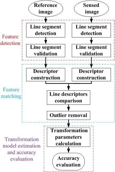
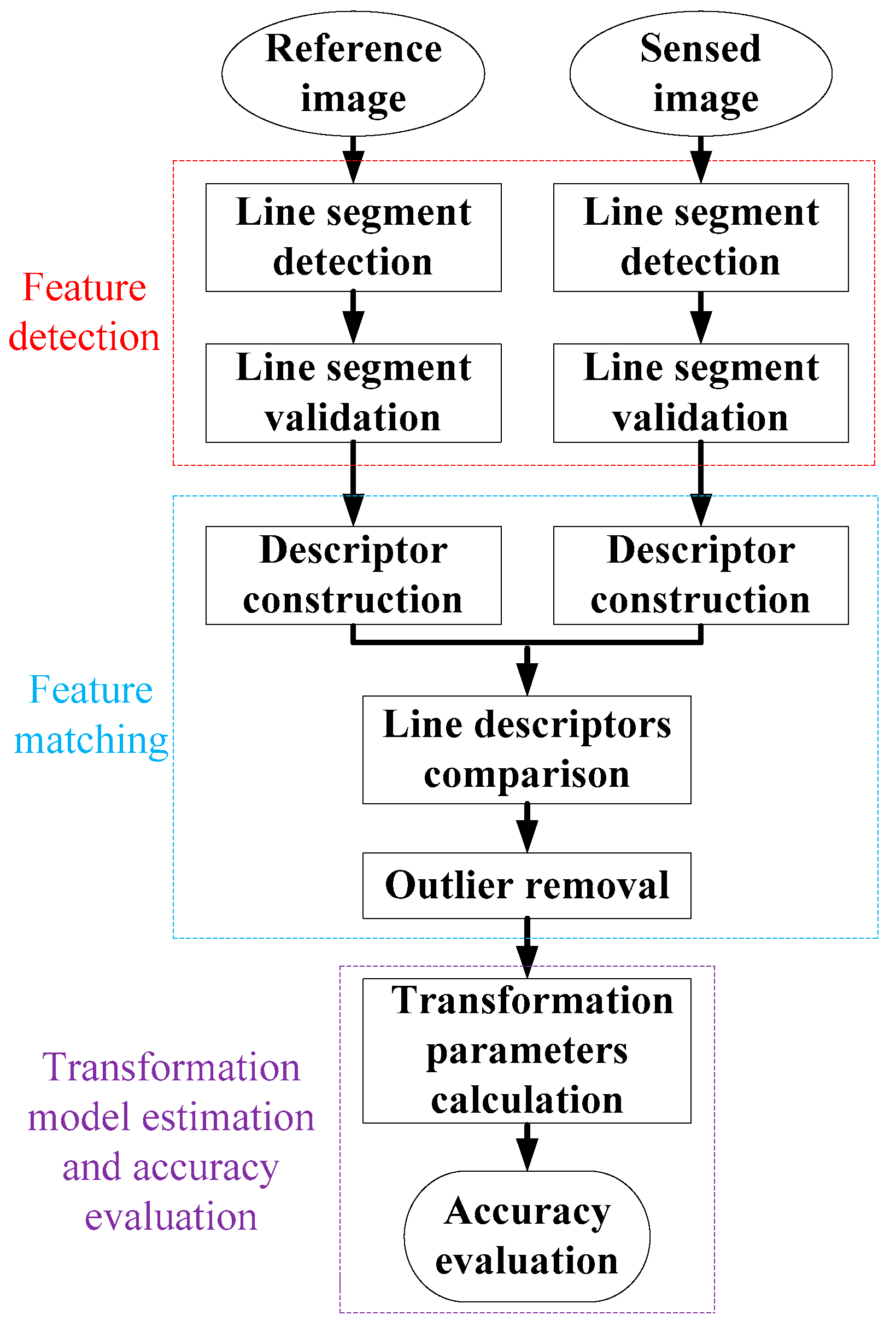
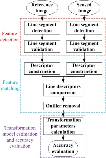
2. Methodology
2.1. Feature Detection
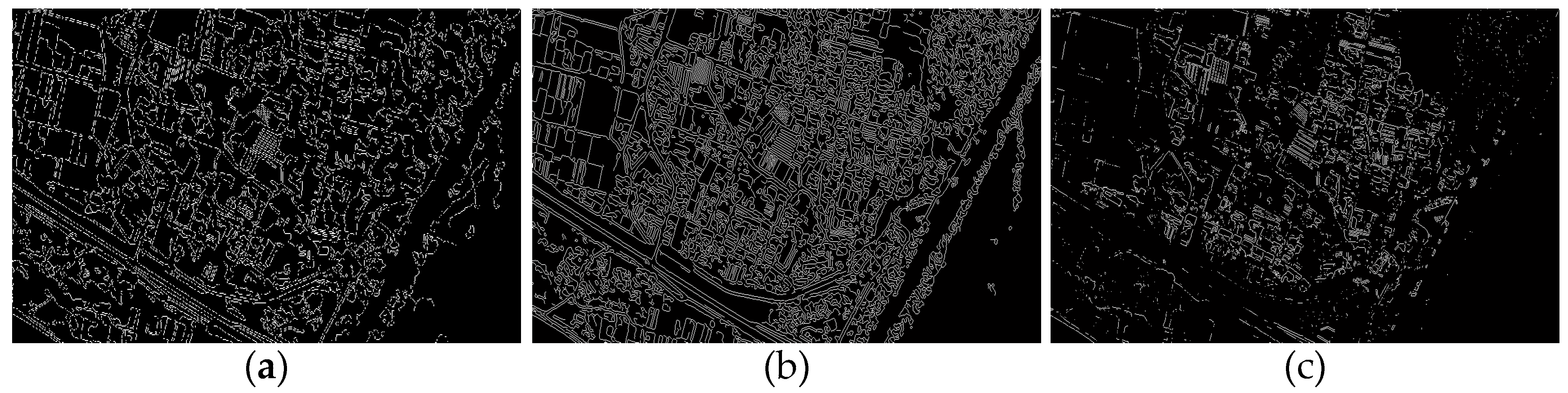
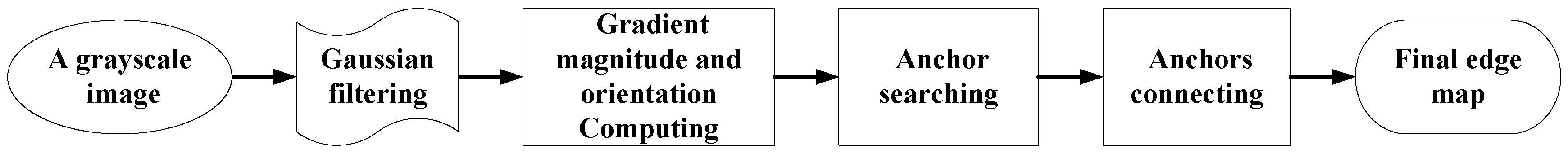
2.1.1. Line Segments’ Detection Using EDLines
2.1.2. Line Segments’ Validation
2.2. Feature Matching
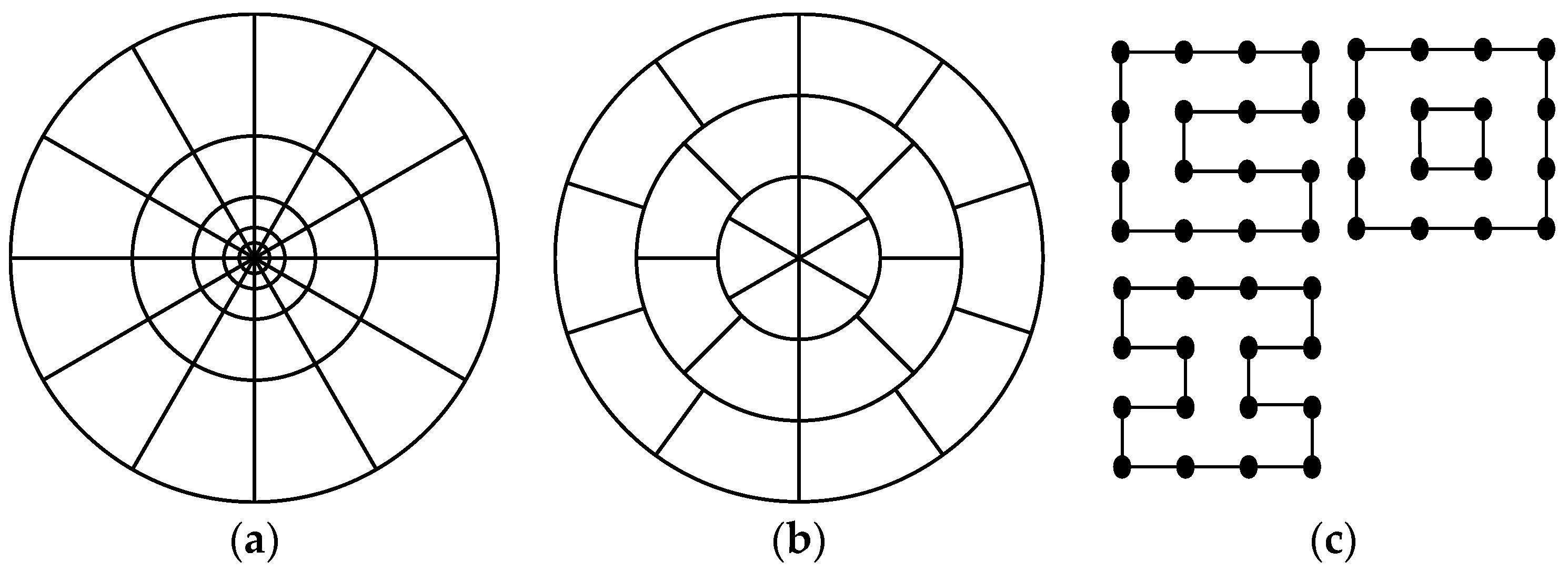
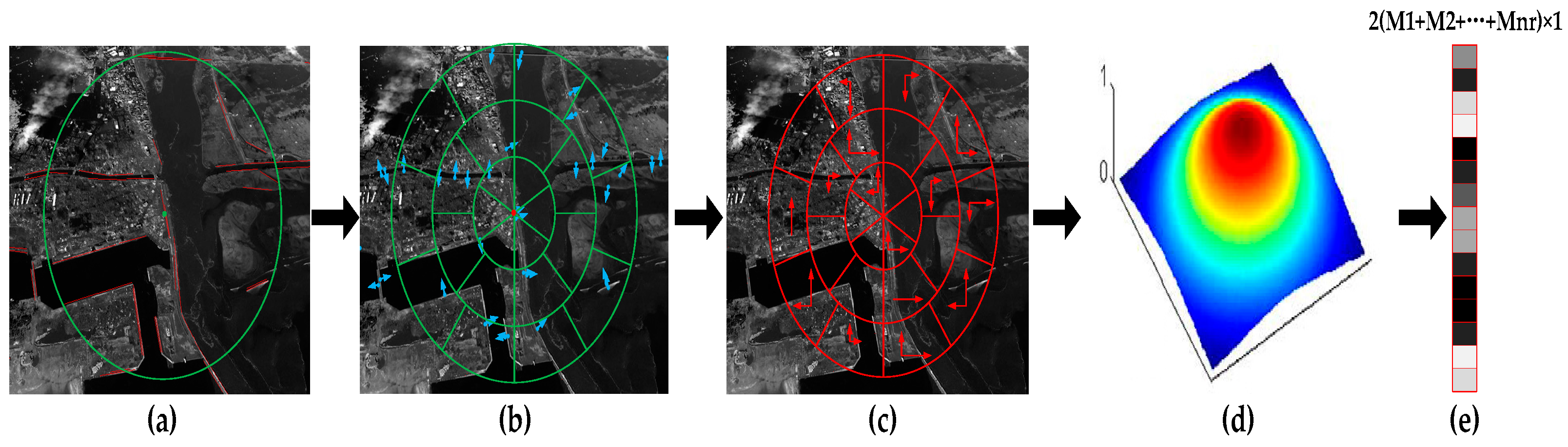
2.2.1. Feature Descriptor
2.2.2. A Spatial Consistency Measure
2.3. Transformation Model Estimation
2.4. Accuracy Evaluation
3. Experiments and Results
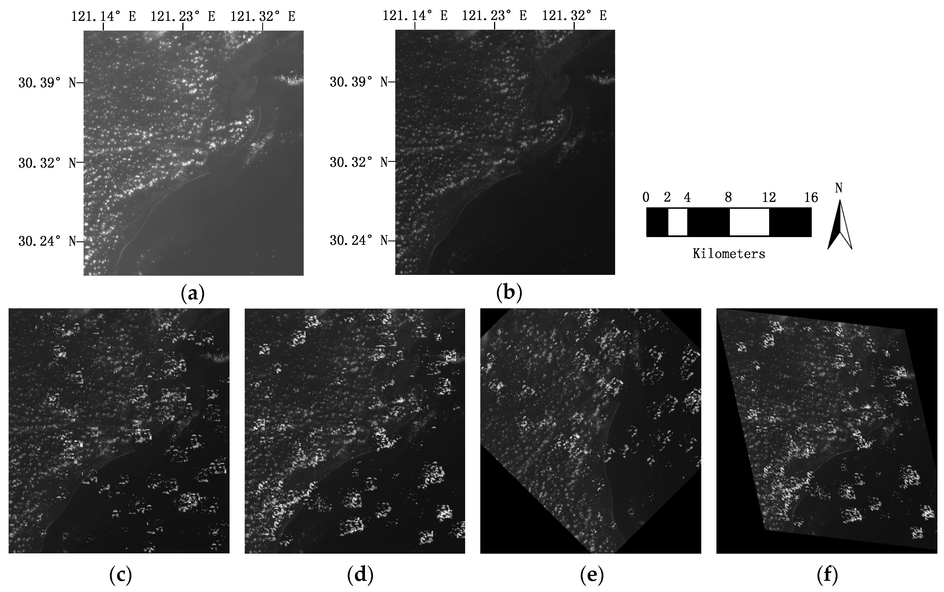
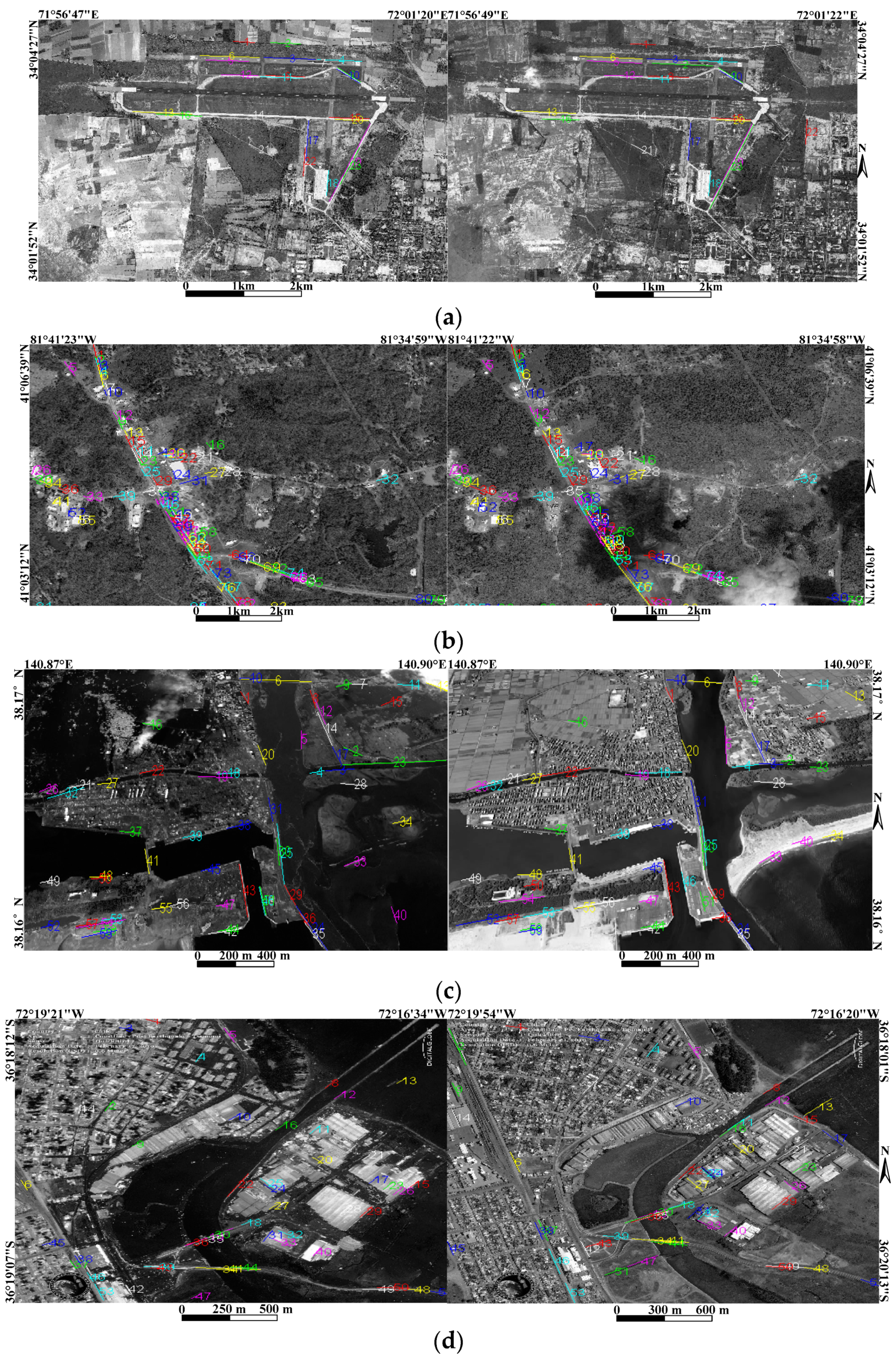
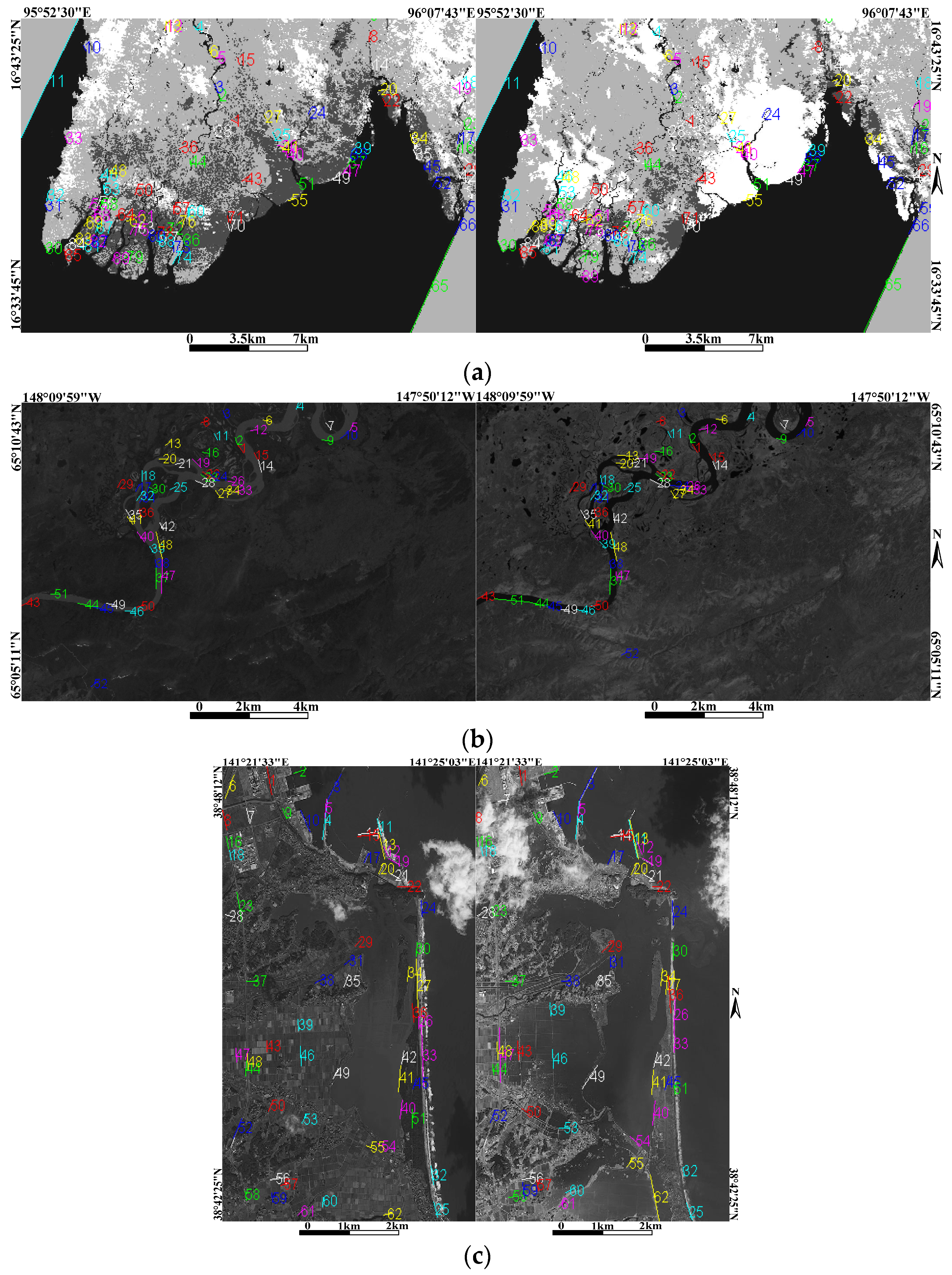
3.1. Image Datasets
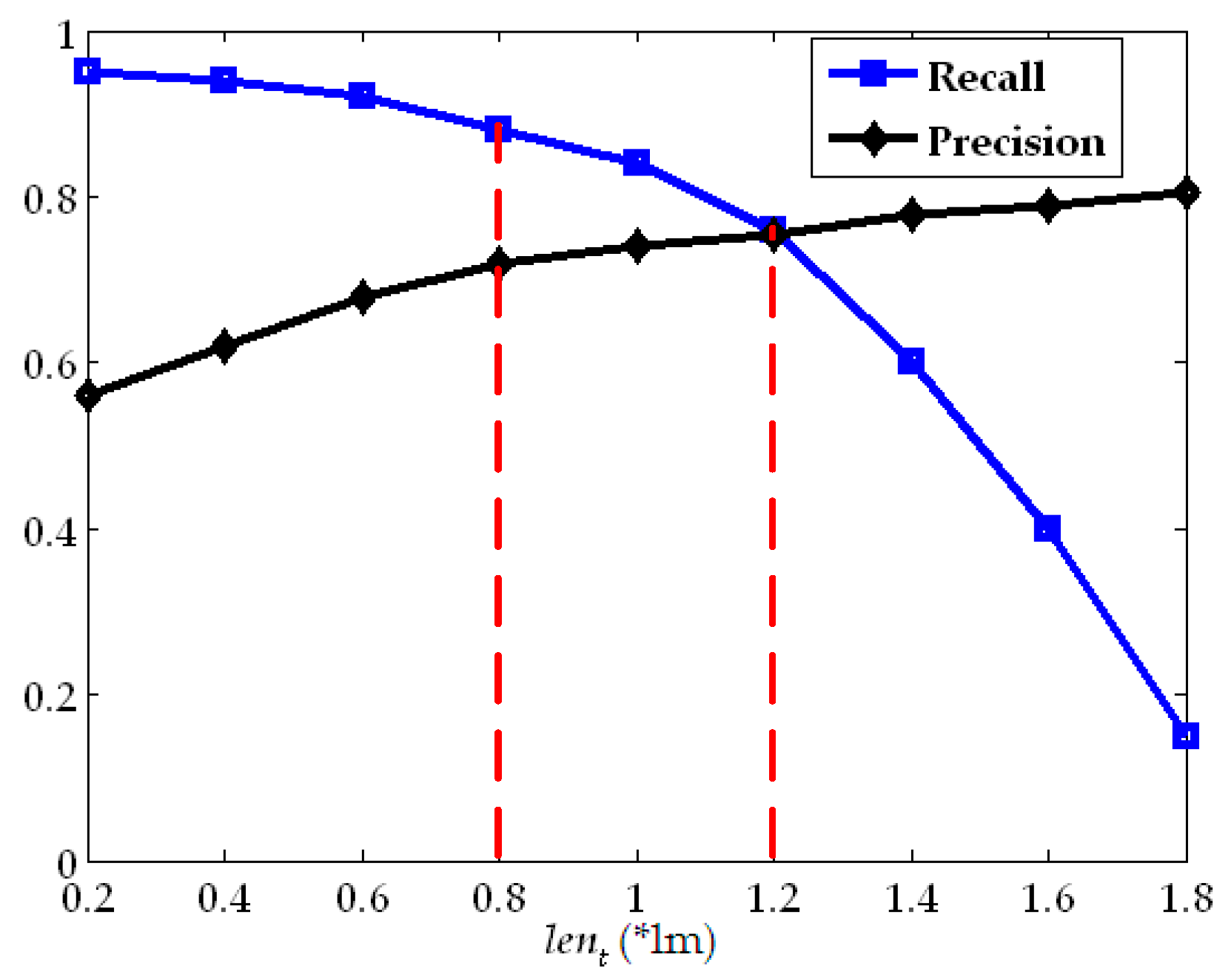
3.2. Parameter Setting
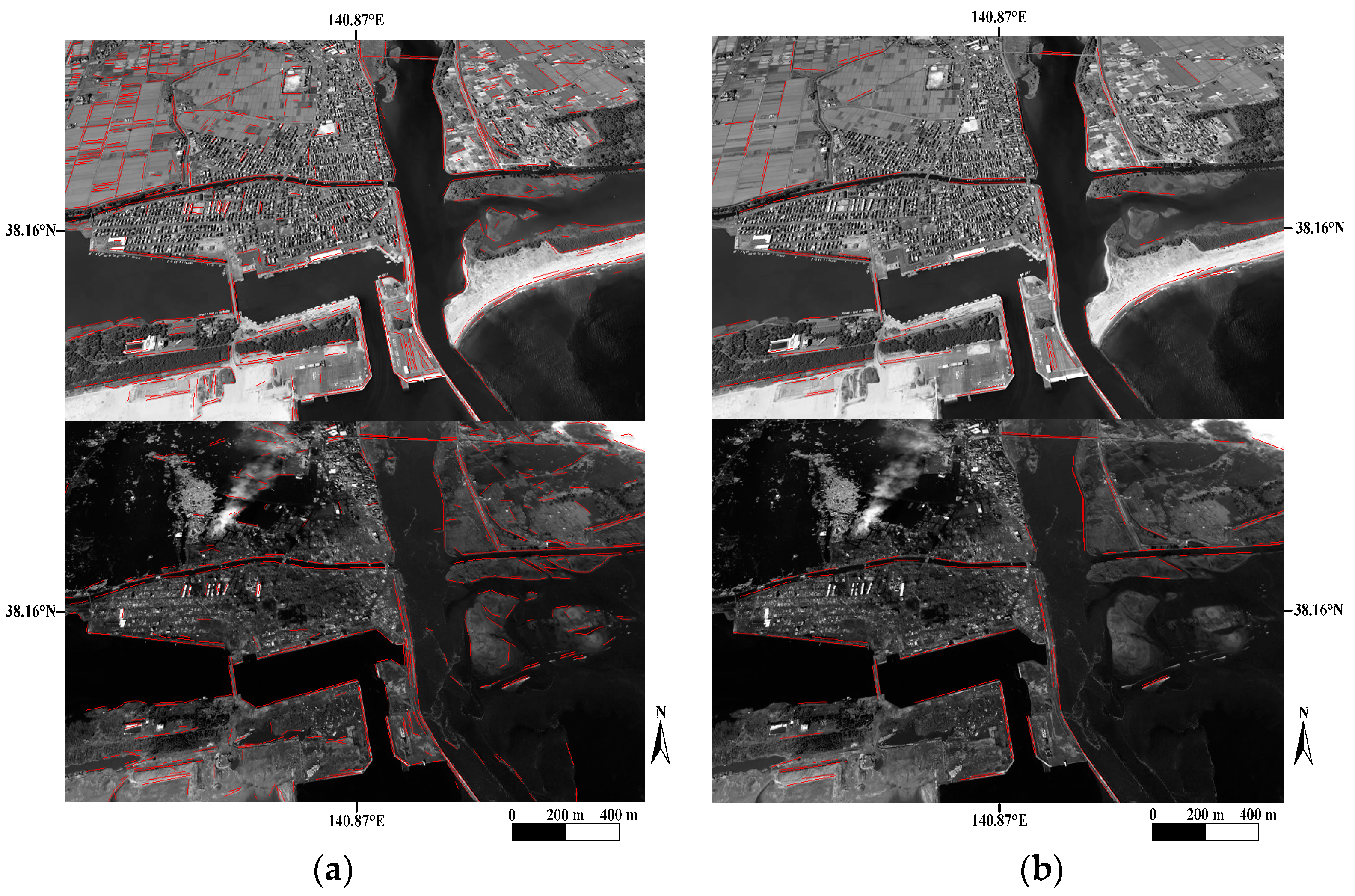
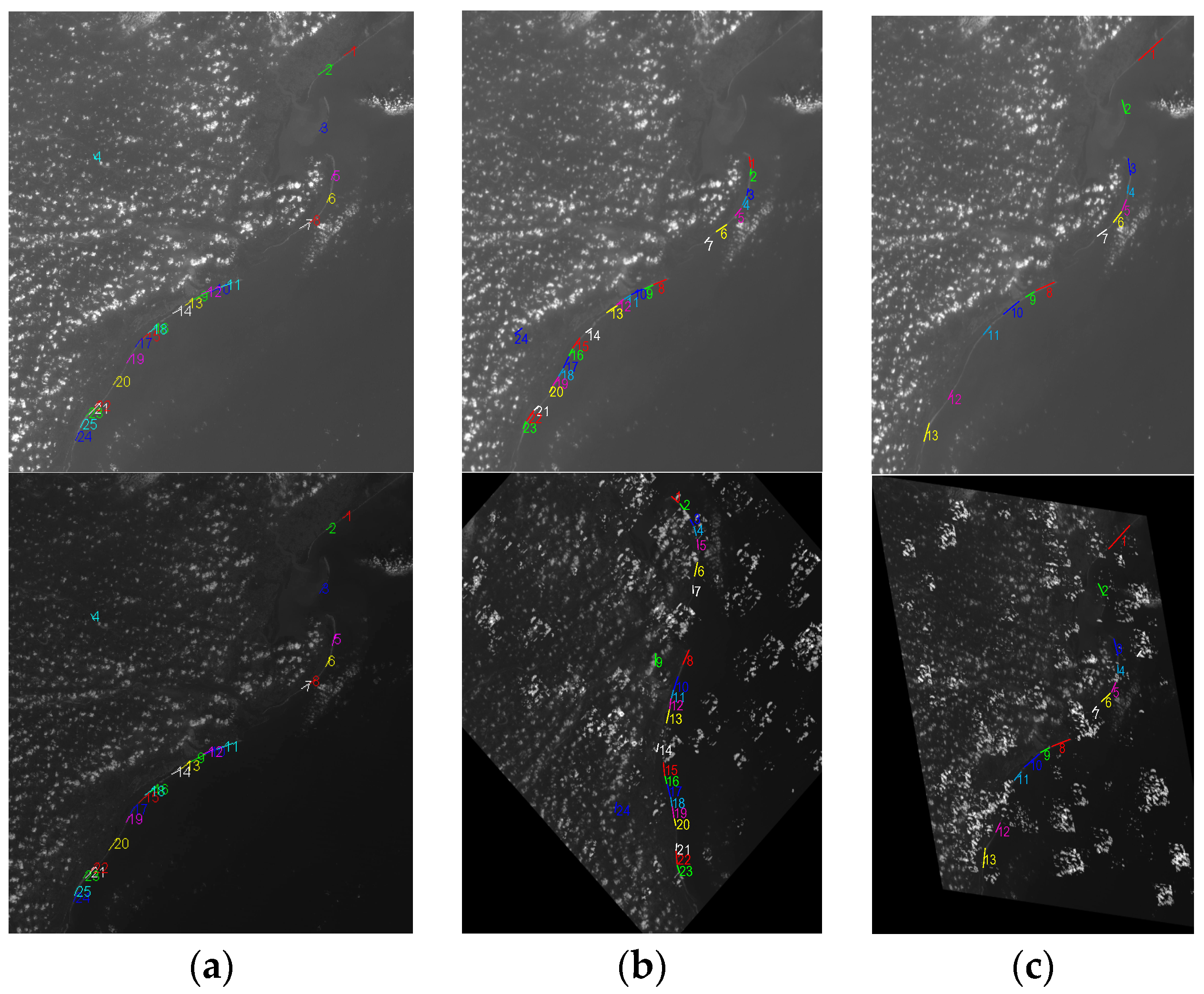
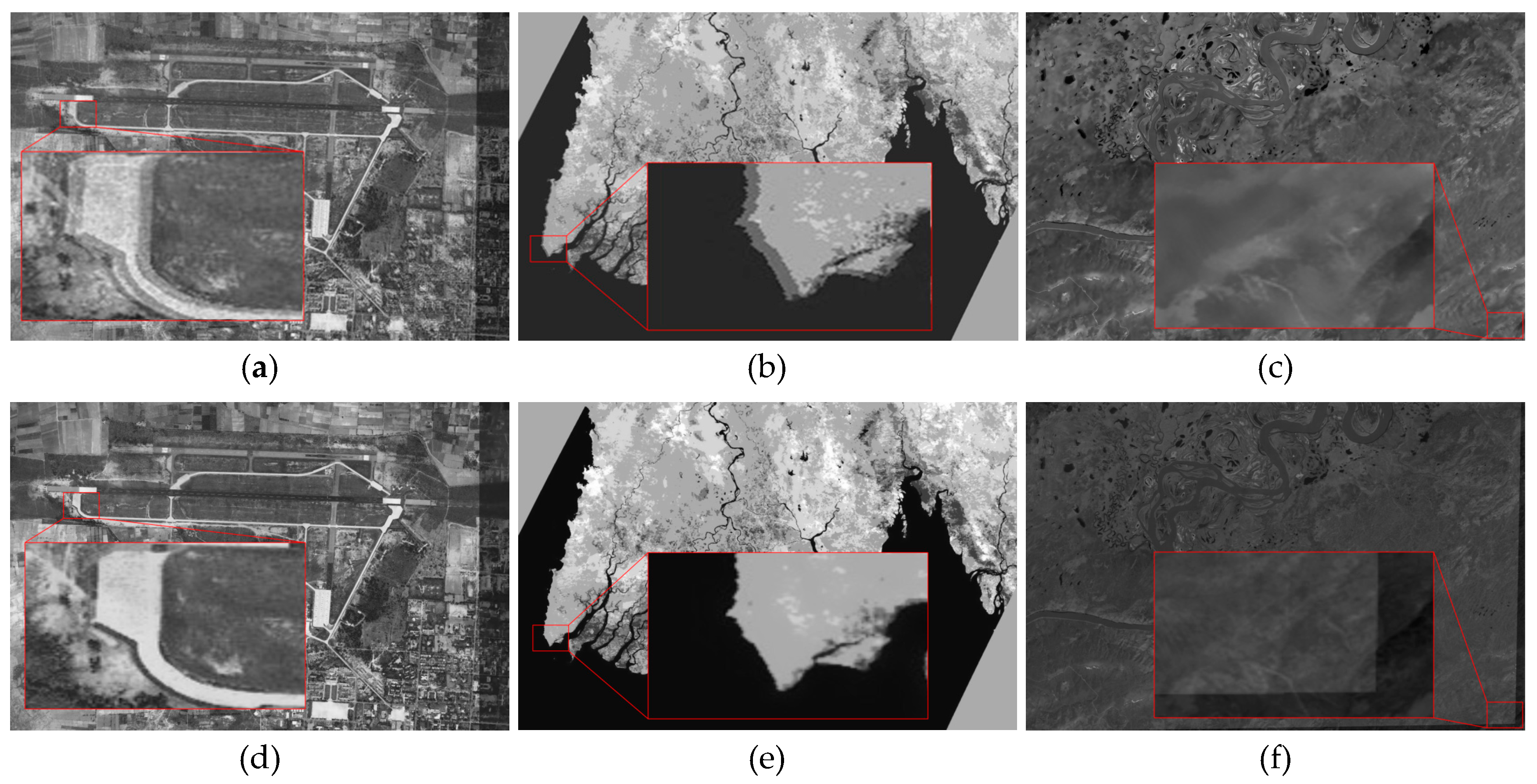
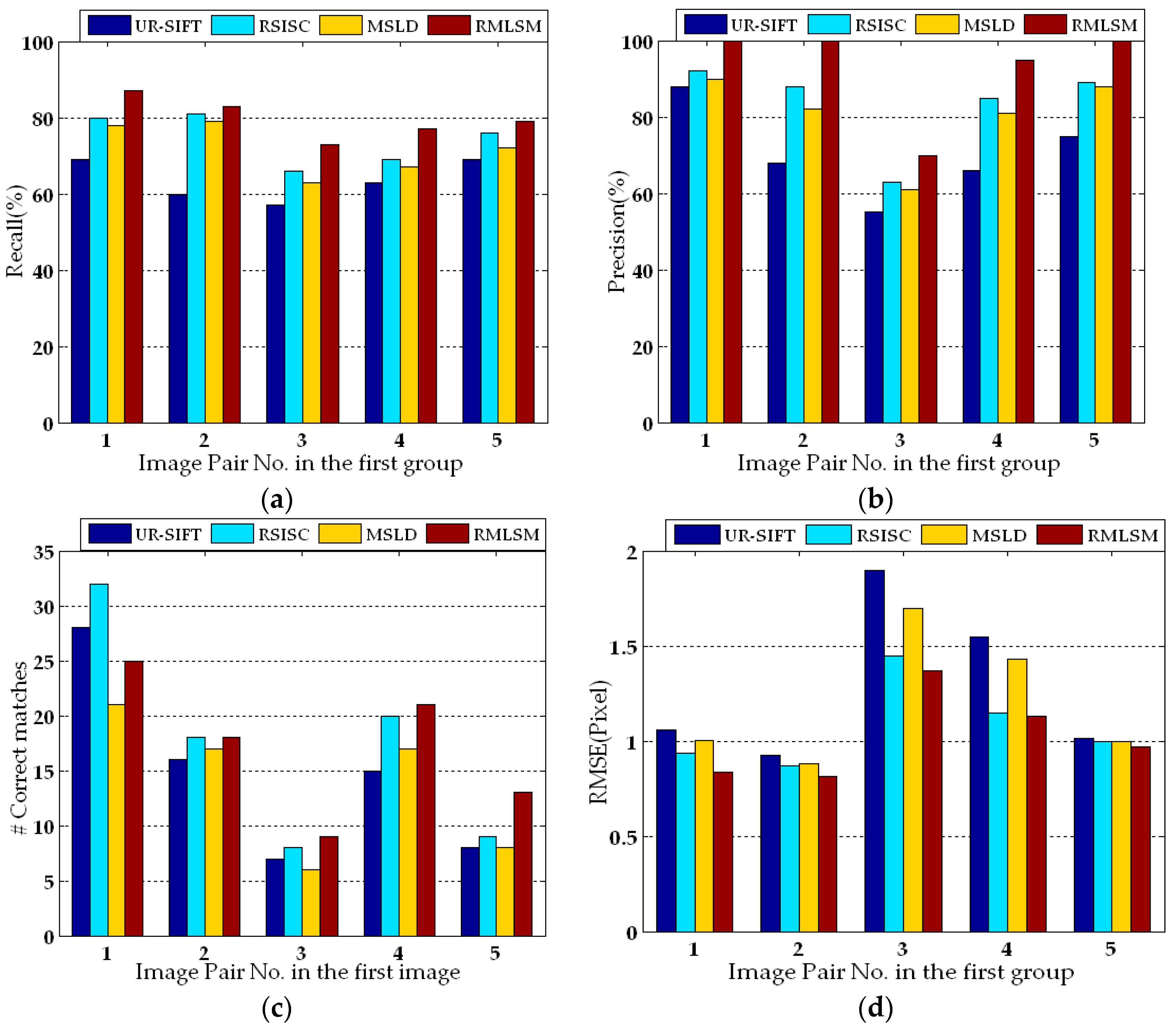
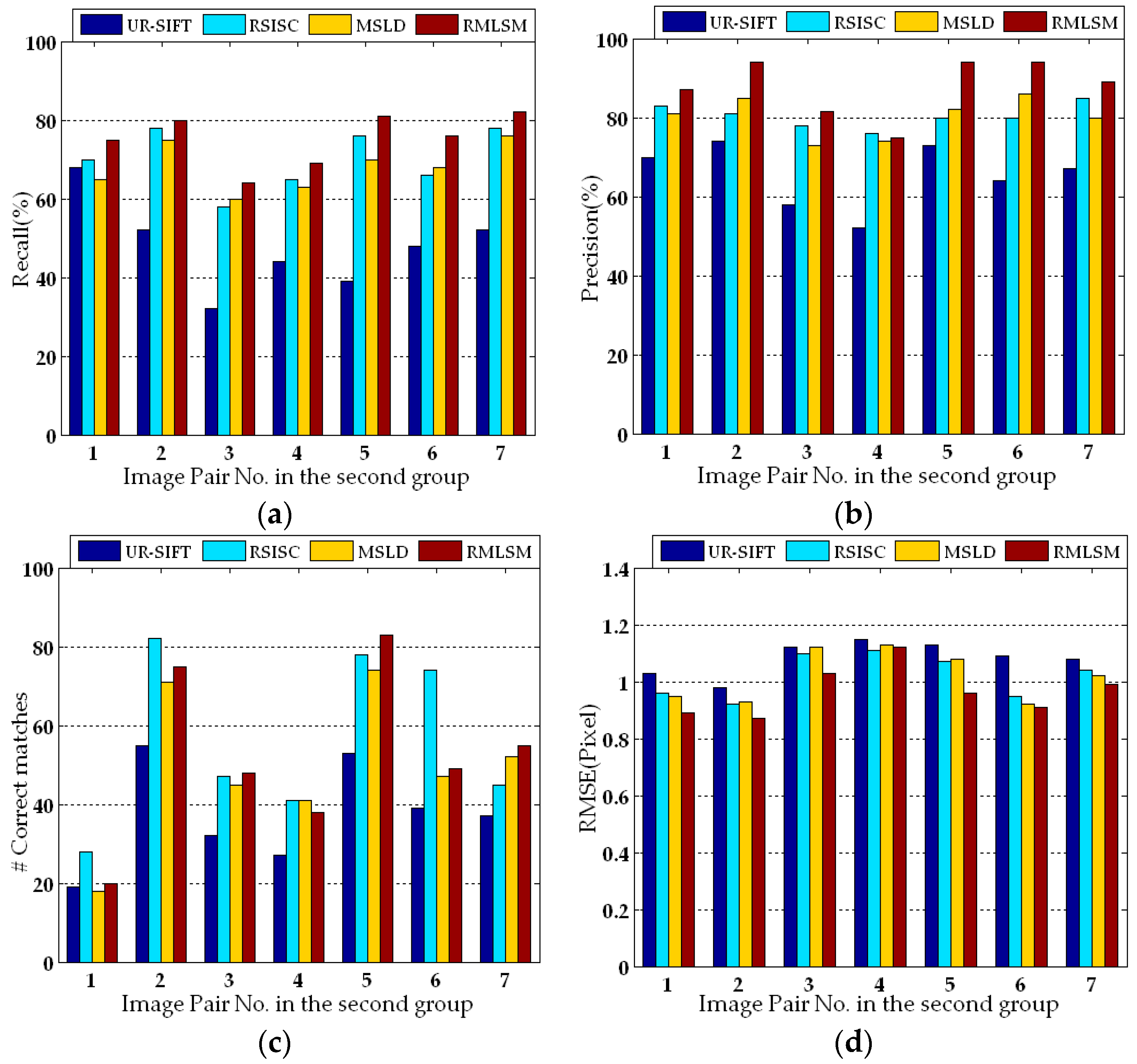
3.3. Experimental Results
4. Discussion
5. Conclusions
Acknowledgments
Author Contributions
Conflicts of Interest
References
- Zitová, B.; Flusser, J. Image registration methods: A survey. Image Vis. Comput. 2003, 21, 977–1000. [Google Scholar] [CrossRef]
- Dawn, S.; Saxena, V.; Sharma, B. Remote sensing image registration techniques: A survey. In Image and Signal Processing; Springer: Berlin/Heidelberg, Germany, 2010; Volume 6134, pp. 103–112. [Google Scholar]
- Slomka, P.J. Multimodality image registration with software: State-of-the-art. Eur. J. Nucl. Med. Mol. Imag. 2009, 36, 44–55. [Google Scholar] [CrossRef] [PubMed]
- Salvi, J.; Matabosch, C.; Fofi, D.; Forest, J. A review of recent range image registration methods with accuracy evaluation. Image Vis. Comput. 2007, 25, 578–596. [Google Scholar] [CrossRef]
- Qin, R.; Gruen, A. 3D change detection at street level using mobile laser scanning point clouds and terrestrial images. ISPRS J. Photogramm. Remote Sens. 2014, 90, 23–35. [Google Scholar] [CrossRef]
- Ardila, J.P.; Bijker, W.; Tolpekin, V.A.; Stein, A. Multitemporal change detection of urban trees using localized region-based active contours in VHR images. Remote Sens. Environ. 2012, 124, 413–426. [Google Scholar] [CrossRef]
- Nebiker, S.; Lack, N.; Deuber, M. Building change detection from historical aerial photographs using dense image matching and object-based image analysis. Remote Sens. 2014, 6, 8310–8336. [Google Scholar] [CrossRef]
- Honkavaara, E.; Litkey, P.; Nurminen, K. Automatic storm damage detection in forests using high-altitude photogrammetric imagery. Remote Sens. 2013, 5, 1405–1424. [Google Scholar] [CrossRef]
- Mnih, V.; Hinton, G. Learning to label aerial images from noisy data. In Proceedings of the 29th International Conference on Machine Learning, Edinburgh, Scotland, UK, 26 June–1 July 2012; pp. 567–574.
- Parmehr, E.G.; Fraser, C.S.; Zhang, C.; Leach, S. Automatic registration of optical imagery with 3D LiDAR data using statistical similarity. ISPRS J. Photogramm. Remote Sens. 2014, 88, 28–40. [Google Scholar] [CrossRef]
- Lerma, J.L.; Navarro, S.; Cabrelles, M.; Segui, A.E.; Hernández, D. Automatic orientation and 3D modelling from markerless rock art imagery. ISPRS J. Photogramm. Remote Sens. 2013, 76, 64–75. [Google Scholar] [CrossRef]
- Ekhtari, N.; Zoej, M.J.V.; Sahebi, M.R.; Mohammadzadeh, A. Automatic building extraction from LIDAR digital elevation models and Worldview imagery. J. Appl. Remote Sens. 2009, 3. [Google Scholar] [CrossRef]
- Wang, X.; Li, Y.; Wei, H.; Liu, F. An ASIFT-based local registration method for satellite imagery. Remote Sens. 2015, 7, 7044–7061. [Google Scholar] [CrossRef]
- Chen, Q.; Wang, S.; Wang, B.; Sun, M. Automatic registration method for fusion of ZY-1–02C satellite images. Remote Sens. 2014, 6, 157–179. [Google Scholar] [CrossRef]
- Wu, Y.; Ma, W.; Gong, M.; Su, L.; Jiao, L. A novel point-matching algorithm based on fast sample consensus for image registration. IEEE Geosci. Remote Sens. Lett. 2015, 12, 43–47. [Google Scholar] [CrossRef]
- Ma, J.; Zhou, H.; Gao, Y.; Jiang, J.; Tian, J. Robust feature matching for remote sensing image registration via locally linear transforming. IEEE Trans. Geosci. Remote Sens. 2015, 53, 6469–6481. [Google Scholar] [CrossRef]
- Ye, Y.; Shan, J. A local descriptor based registration method for multispectral remote sensing images with non-linear intensity differences. ISPRS J. Photogramm. Remote Sens. 2014, 90, 83–95. [Google Scholar] [CrossRef]
- Linger, M.E.; Goshtasby, A. Aerial image registration for tracking. IEEE Trans. Geosci. Remote Sens. 2015, 53, 2137–2145. [Google Scholar] [CrossRef]
- Zagorchev, L.; Goshtasby, A. A comparative study of transformation functions for nonrigidimage registration. IEEE Trans. Image Process. 2006, 15, 529–538. [Google Scholar] [CrossRef] [PubMed]
- Peter, T.B.B.; Guida, R. Earthquake damage detection in urban areas using curvilinear Features. IEEE Trans. Geosci. Remote Sens. 2013, 51, 4877–4884. [Google Scholar]
- Song, Z.; Zhou, S.; Guan, J. A novel image registration algorithm for remote sensing under affine transformation. IEEE Trans. Geosci. Remote Sens. 2014, 52, 4895–4912. [Google Scholar] [CrossRef]
- Gong, M.; Zhao, S.; Jiao, L.; Tian, D.; Wang, S. A novel coarse-to-fine scheme for automatic image registration based on SIFT and mutual Information. IEEE Trans. Geosci. Remote Sens. 2014, 52, 4328–4338. [Google Scholar] [CrossRef]
- Segaghat, A.; Ebadi, H. Remote sensing image matching based on adaptive binning SIFT descriptor. IEEE Trans. Geosci. Remote Sens. 2015, 53, 5283–5293. [Google Scholar] [CrossRef]
- Cao, S.; Jiang, J.; Zhang, G.; Yuan, Y. An edge-based scale- and affine- invariant algorithm for remote sensing image registration. Int. J. Remote Sens. 2013, 34, 2301–2326. [Google Scholar] [CrossRef]
- Jiang, J.; Cao, S.; Zhang, G.; Yuan, Y. Shape registration for remote-sensing images with background variation. Int. J. Remote Sens. 2013, 34, 5265–5281. [Google Scholar] [CrossRef]
- Lowe, D. Distinctive image features from scale-invariant keypoints. Int. J. Comput. Vis. 2004, 60, 91–110. [Google Scholar] [CrossRef]
- Bay, H.; Ess, A.; Tuytelaars, T.; Gool, L.C. Speeded-up robust features (SURF). Comput. Vis. Image Underst. 2008, 110, 346–359. [Google Scholar] [CrossRef]
- Mikolajczyk, K.; Schmid, C. A performance evaluation of local descriptors. IEEE Trans. Pattern Anal. Mach. Intell. 2005, 27, 1615–1630. [Google Scholar] [CrossRef] [PubMed]
- Morel, J.M.; Yu, G. ASIFT: A new framework for fully affine invariant image comparison. SIAM J. Imaging Sci. 2009, 2, 438–469. [Google Scholar] [CrossRef]
- Bradley, P.E.; Jutzi, B. Improved feature detection in fused intensity-range images with complex SIFT. Remote Sens. 2011, 3, 2076–2088. [Google Scholar] [CrossRef]
- Segaghat, A.; Mokhtarzade, M.; Ebadi, H. Uniform robust scale-invariant feature matching for optical remote sensing images. IEEE Trans. Geosci. Remote Sens. 2011, 49, 4516–4527. [Google Scholar] [CrossRef]
- Ghosh, P.; Manjunath, B.S. Robust simultaneous registration and segmentation with sparse error reconstruction. IEEE Trans. Pattern Anal. Mach. Intell. 2013, 35, 425–436. [Google Scholar] [CrossRef] [PubMed]
- Arandjelović, O.; Pham, D.; Venkatesh, S. Efficient and accurate set-based registration of time-separated aerial images. Pattern Recognit. 2015, 48, 3466–3476. [Google Scholar] [CrossRef]
- Tanathong, S.; Lee, I. Using GPS/INS data to enhance image matching for real-time aerial triangulation. Comput. Geosci. 2014, 72, 244–254. [Google Scholar] [CrossRef]
- Konstantin, V.; Alexander, P.; Yi, L. Achieving subpixel georeferencing accuracy in the canadian AVHRR processing system. IEEE Trans. Geosci. Remote Sens. 2010, 48, 2150–2161. [Google Scholar]
- Belongie, S.; Malik, J.; Puzicha, J. Shape matching and object recognition using shape context. IEEE Trans. Pattern Anal. Mach. Intell. 2002, 24, 509–522. [Google Scholar] [CrossRef]
- Lei, H.; Zhen, L. Feature-based image registration using the shape context. Int. J. Remote Sens. 2010, 31, 2169–2177. [Google Scholar]
- Jiang, J.; Zhang, S.; Cao, S. Rotation and scale invariant shape context registration for remote sensing images with background variations. J. Appl. Remote Sens. 2015, 9, 92–110. [Google Scholar] [CrossRef]
- Arandjelović, O. Object matching using boundary descriptors. In Proceedings of the British Machine Vision Conference, Surrey, UK, 3–7 September 2012.
- Arandjelović, O. Gradient edge map features for frontal face recognition under extreme illumination changes. In Proceedings of the British Machine Vision Conference, Surrey, UK, 3–7 September 2012.
- Wang, Z.; Wu, F.; Hu, Z. MSLD: A robust descriptor for line matching. Pattern Recognit. 2009, 42, 941–953. [Google Scholar] [CrossRef]
- Zhang, L.; Koch, R. An efficient and robust line segment matching approach based on LBD descriptor and pairwise geometric consistency. J. Vis. Commun. Image Represent. 2013, 24, 794–805. [Google Scholar] [CrossRef]
- López, J.; Santos, R.; Fdez-Vidal, X.R.; Pardo, X.M. Two-view line matching algorithm based on context and appearance in low-textured images. Pattern Recognit. 2015, 48, 2164–2184. [Google Scholar] [CrossRef]
- Akinlar, C.; Topal, C. EDLines: A real-time line segment detector with a false detection control. Pattern Recognit. Lett. 2011, 32, 1633–1642. [Google Scholar] [CrossRef]
- Topal, C.; Akinlar, C. Edge Drawing: A combined real-time edge and segment detector. J. Vis. Commun. Image Represent. 2012, 23, 862–872. [Google Scholar] [CrossRef]
- Desolneux, A.; Moisan, L.; Morel, J.M. Meaningfull alignments. Int. J. Comput. Vis. 2000, 40, 7–23. [Google Scholar] [CrossRef]
- Desolneux, A.; Moisan, L.; Morel, J.M. From Gestalt Theory to Image Analysis: A Probabilistic Approach; Springer: New York, NY, USA, 2008. [Google Scholar]
- Li, A.; Cheng, X.; Guan, H.; Feng, T.; Guan, Z. Novel image registration method based on local structure constraints. IEEE Geosci. Remote Sens. Lett. 2014, 11, 1584–1588. [Google Scholar]


| Algorithm 1: Algorithm to extract line segments |
| FitLines(Pixel * pixelChain, intpixels_num) |
| { |
| doubleError_LineFit=INFINITY; // current line fit error |
| Line_Equationline_equation; // y=ax+b or x=ay+b |
| while(pixels_num>MIN_LINE_DISTANCE) |
| { |
| LeastSquareFitLine(pixelChain, MIN_LINE_DISTANCE, &line_equation, &Error_LineFit); |
| if(Error_LineFit<=1.0) break; // An initial line segment detected |
| pixelChain++; |
| pixels_num--; |
| } // end-while |
| if(Error_LineFit>1.0) return; // no initial line segment |
| // if an initial line segment has detected |
| intlineLen= MIN_LINE_DISTANCE; |
| while(lineLen<pixels_num) |
| { |
| double d=ComputePointDistanceToLine(line_equation, pixelChain[lineLen]); |
| if(d>1.0) break; |
| lineLen++; |
| } // end-while |
| // output current line equation |
| LeastSquareFitLine(pixelChain, lineLen, &line_equation); |
| Output “line_equation” |
| FitLines(pixelChain+lineLen, pixel_num-lineLen); // Extract line segments from the remain pixels |
| } //end-FitLines |
| Group | No. | Location | Image Size | Bits | GSD(m) | Date | Sensor | Events |
|---|---|---|---|---|---|---|---|---|
| Simulatedimages | 1-1 | Hangzhou | 2129 × 2373 | 8 | 30 | 2011 | Landsat5 | Band1 |
| Hangzhou | 2129 × 2373 | 8 | 30 | 2011 | Landsat5 | Band2 | ||
| High-resolution real images | 2-1 | Pakistan | 1817 × 1194 | 11 | 2 | 2007 | QuickBird | Pre-flood |
| Pakistan | 1739 × 1056 | 11 | 2 | 2010 | WorldView | Post-flood | ||
| 2-2 | Mississippi | 4254 × 3646 | 11 | 0.61 | 2010 | QuickBird | Pre-tornado | |
| Mississippi | 4254 × 3647 | 11 | 0.61 | 2010 | QuickBird | Post-tornado | ||
| 2-3 | Natori | 940 × 529 | 11 | 0.61 | 2007 | QuickBird | Pre-tsunami | |
| Natori | 940 × 529 | 11 | 0.61 | 2011 | QuickBird | Post-tsunami | ||
| 2-4 | Chile | 2559 × 2528 | 11 | 0.61 | 2010 | QuickBird | Pre-tsunami | |
| Chile | 2566 × 2621 | 11 | 0.61 | 2010 | QuickBird | Post-tsunami | ||
| Medium- and low-resolution real images | 2-5 | Myanmar | 1800 × 1200 | 8 | 231.65 | 2008 | Aqua | Pre-flood |
| Myanmar | 1687 × 1081 | 8 | 231.65 | 2008 | Aqua | Post-flood | ||
| 2-6 | Alaska | 1800 × 1200 | 8 | 30 | 2004 | Landsat7 | Band 3 | |
| Alaska | 1800 × 1200 | 8 | 30 | 2004 | Landsat7 | Band 4 | ||
| 2-7 | Fukushima | 584 × 923 | 8 | 10 | 2009 | SPOT 4 | Pre-tsunami | |
| Fukushima | 728 × 1064 | 8 | 10 | 2011 | SPOT 4 | Post-tsunami |
| Parameter Setting | Recall (%) | Precision (%) | Descriptor Dimension |
|---|---|---|---|
| 65.2 | 73.1 | 36 | |
| 69.7 | 77.3 | 44 | |
| 76.0 | 82.4 | 56 | |
| 77.4 | 84.0 | 68 | |
| 81.7 | 86.4 | 80 | |
| 80.1 | 87.6 | 96 | |
| 82.5 | 91.1 | 108 | |
| 83.7 | 90.9 | 128 | |
| 84.2 | 91.4 | 140 | |
| 84.7 | 92.5 | 164 |
| Recall/Precision | No. 2-1 | No. 2-2 | No. 2-3 | No. 2-4 | No. 2-5 | No. 2-6 | No. 2-7 |
|---|---|---|---|---|---|---|---|
| RMLSM | 75.2%/86.9% | 80.5%/93.1% | 65.6%/81.4% | 68.7%/70.4% | 81.8%/94.1% | 76.7%/93.7% | 82.4%/90.2% |
| SC | 71.2%/80.4% | 74.6%/83.2% | 67.2%/78.4% | 67.0%/65.1% | 73.2%/82.0% | 70.7%/84.4% | 77.3%/81.6% |
© 2016 by the authors; licensee MDPI, Basel, Switzerland. This article is an open access article distributed under the terms and conditions of the Creative Commons Attribution (CC-BY) license (http://creativecommons.org/licenses/by/4.0/).
Share and Cite
Shi, X.; Jiang, J. Automatic Registration Method for Optical Remote Sensing Images with Large Background Variations Using Line Segments. Remote Sens. 2016, 8, 426. https://doi.org/10.3390/rs8050426
Shi X, Jiang J. Automatic Registration Method for Optical Remote Sensing Images with Large Background Variations Using Line Segments. Remote Sensing. 2016; 8(5):426. https://doi.org/10.3390/rs8050426
Chicago/Turabian StyleShi, Xiaolong, and Jie Jiang. 2016. "Automatic Registration Method for Optical Remote Sensing Images with Large Background Variations Using Line Segments" Remote Sensing 8, no. 5: 426. https://doi.org/10.3390/rs8050426