Article

Analysis of Red and Far-Red Sun-Induced Chlorophyll Fluorescence and Their Ratio in Different Canopies Based on Observed and Modeled Data

1
Remote Sensing of Environmental Dynamics Laboratory, Department of Earth and Environmental Science (DISAT), University of Milano-Bicocca, Piazza della Scienza 1, 20126 Milano, Italy
2
European Commission, Joint Research Centre, Institute for Environment and Sustainability, Monitoring Agricultural Resources Unit, via Fermi 2749, 21027 Ispra, VA, Italy
3
Institute of Bio- and Geosciences, IBG-2: Plant Sciences, Forschungszentrum Jülich GmbH, Leo-Brandt-Str., 52425 Jülich, Germany
4
Department of Water Resources, Faculty ITC, University of Twente, 7500 Enschede, The Netherlands
*
Author to whom correspondence should be addressed.
Remote Sens. 2016, 8(5), 412; https://doi.org/10.3390/rs8050412
Submission received: 7 October 2015 / Revised: 4 May 2016 / Accepted: 9 May 2016 / Published: 13 May 2016
(This article belongs to the Special Issue Field Spectroscopy and Radiometry)

Abstract

:
Sun-induced canopy chlorophyll fluorescence in both the red (FR) and far-red (FFR) regions was estimated across a range of temporal scales and a range of species from different plant functional types using high resolution radiance spectra collected on the ground. Field measurements were collected with a state-of-the-art spectrometer setup and standardized methodology. Results showed that different plant species were characterized by different fluorescence magnitude. In general, the highest fluorescence emissions were measured in crops followed by broadleaf and then needleleaf species. Red fluorescence values were generally lower than those measured in the far-red region due to the reabsorption of FR by photosynthetic pigments within the canopy layers. Canopy chlorophyll fluorescence was related to plant photosynthetic capacity, but also varied according to leaf and canopy characteristics, such as leaf chlorophyll concentration and Leaf Area Index (LAI). Results gathered from field measurements were compared to radiative transfer model simulations with the Soil-Canopy Observation of Photochemistry and Energy fluxes (SCOPE) model. Overall, simulation results confirmed a major contribution of leaf chlorophyll concentration and LAI to the fluorescence signal. However, some discrepancies between simulated and experimental data were found in broadleaf species. These discrepancies may be explained by uncertainties in individual species LAI estimation in mixed forests or by the effect of other model parameters and/or model representation errors. This is the first study showing sun-induced fluorescence experimental data on the variations in the two emission regions and providing quantitative information about the absolute magnitude of fluorescence emission from a range of vegetation types.

Graphical Abstract

1. Introduction

Interest in remote sensing of sun-induced chlorophyll fluorescence emitted by terrestrial vegetation in the red (FR) and far-red (FFR) regions is motivated by the causal relation between fluorescence and actual plant photosynthesis [1].
Under natural sunlight illumination, the amount of chlorophyll fluorescence emitted by terrestrial vegetation is a small fraction of the radiation reflected by a plant in the red and near-infrared spectral regions. However, the fluorescence signal can be quantified by passive (i.e., without artificial excitation sources) remote sensing systems exploiting dark regions of the solar and atmospheric spectrum in which irradiance is strongly reduced. In particular, two telluric O2 absorption bands (O2-B band at 687 nm and O2-A band at 760.4 nm) were extensively used to estimate sun-induced fluorescence because of their spectral proximity to the peaks of the fluorescence emission spectrum positioned at about 685 and 740 nm [2].
Global maps of sun-induced chlorophyll fluorescence in the far-red region are becoming increasingly available from satellites [3,4,5] designed for atmospheric studies. Such instruments have spatial and temporal resolutions that are unsuited for vegetation studies [6]. This makes a proper validation of the fluorescence maps over terrestrial ecosystems not feasible. In this context, the ground-based characterization of different plant functional types at different spatial and temporal scales can be extremely useful for the evaluation of reliable ranges of variation for fluorescence retrieval and for a better understanding of the main factors inducing fluorescence modulation in both space and time.
Whilst the feasibility to detect the FFR signal was demonstrated at different scales [7,8,9,10], only few studies successfully retrieved canopy FR [11,12]. This is because the majority of available instruments have a coarse spectral resolution combined with a low signal-to-noise ratio that make it difficult to resolve the width of the narrow O2-B band and properly retrieve the faint FR signal.
Based on a modeling study, Verrelst et al. [13] showed that a part of the fluorescence variability can be related to variations in leaf chlorophyll concentration and vegetation structure as expressed by leaf area index (LAI) and leaf inclination distribution, while photosynthetic capacity can be less influential in driving the fluorescence signal, particularly in the far-red region. Thus, the structural effects must be taken into consideration to disentangle the contribution of the photosynthetic capacity and correctly interpret fluorescence measurements.
Here, we analyze the variables driving fluorescence emission in the red and far-red region using a wide dataset of sun-induced canopy chlorophyll fluorescence measurements collected on the ground in the last 10 years across a range of different species, in order to address the following research questions: what are the ranges of variation of FFR and FR in terrestrial ecosystems? What are the main factors affecting fluorescence variations? What is the relationship between FFR and FR across different plant species?
The comparison of FFR and FR values is made possible here for the first time due to the availability of a large sun-induced fluorescence dataset collected with a specific and fixed state-of-the-art high resolution spectrometer setup and standardized methodology allowing the comparison of measurements collected at different times and locations, minimizing possible confounding effects due to different experimental setups. Variations in fluorescence emission values related to measurement techniques, type of instrument and setups are not negligible [14]. Damm et al. [15] showed how the accuracy of fluorescence retrievals is affected by the spectral and radiometric resolution of the instruments used. The method used to estimate F may also have an impact on the fluorescence retrievals, as demonstrated by Alonso et al. [16], who showed that overestimation by the standard FLD (Fraunhofer Line Discrimination) method is a direct consequence of its working hypotheses, regardless of the instrument used. These effects were already clearly evident in the first attempt to review and compare FR and FFR magnitudes collected in the context of different experiments published in Meroni et al. [2], where the range of variation of fluorescence retrievals was likely driven by the instrument used for the retrieval.
In this contribution, measurements were collected using spectrometers with a sub-nanometer resolution in the O2-B and O2-A spectral regions. Such fine resolution enabled the application of the so-called spectral fitting methods (SFMs) [17] to estimate sun-induced fluorescence. This technique has been extensively tested and was selected as the method to be implemented for fluorescence retrieval for the European Space Agency’s (ESA’s) Fluorescence Explorer (FLEX) mission, recently selected as the 8th Earth Explorer mission.
Findings based on empirical ground-based results were compared to radiative transfer model simulations of the Soil-Canopy Observation of Photochemistry and Energy fluxes (SCOPE) model [18] in order to isolate and better understand the contribution of two main canopy parameters (i.e., leaf chlorophyll concentration and LAI) to the fluorescence signal.

2. Materials and Methods

2.1. Ground Measurements of High Resolution Top-of-Canopy Radiance

Canopy leaving radiances were measured with three portable spectrometers (two HR4000 and one QE65000, OceanOptics, Dunedin, FL, USA) operating in the visible and near-infrared regions with different spectral resolution. The first instrument (HR4000) covers the 400–1000 nm spectral range with a full width at half maximum (FWHM) of 1 nm and allows the computation of different vegetation indices and incident Photosynthetic Photon Flux Density (PPFD). In particular, the normalized difference vegetation index (NDVI, [19]) and the MERIS terrestrial chlorophyll index (MTCI, [20]) were computed (Equations (1) and (2)) and used in the following analyses.
N D V I =   R 800 R 680 R 800 + R 680
M T C I =   R 753.75 R 708.75 R 708.75 R 681.25
where R is the reflectance at the specified wavelength (nm).
The other two spectrometers are specifically intended for fluorescence measurement: a spectrometer QE65000 operating in the 657–740 nm spectral range with a FWHM of 0.25 nm, dynamic range of 16 bit and a nominal signal-to-noise ratio of 1000 was used to estimate sun-induced fluorescence at the O2-B absorption band and a HR4000 spectrometer covering the spectral region from 700 to 800 nm with a FWHM of 0.1 nm (dynamic range of 14 bit and a nominal signal-to-noise ratio of 300) was used to estimate sun-induced fluorescence at the O2-A absorption band. Spectrometers were housed in a Peltier thermally regulated box (model NT-16, Magapor, Zaragoza, Spain) keeping the internal temperature at 25 °C in order to ensure the stability of both the intensity and the spectral information of the measured signal. The average canopy plane was always observed from nadir with bare fibers (field of view of 25°) at a distance between 100 and 450 cm from the top of the canopy. The manual rotation of a horizontally mounted mast allowed observing alternatively the vegetated target or the white reference calibrated panel (Labsphere Inc., North Sutton, NH, USA).
Target measurements were sandwiched between two white reference panel measurements made by a single device a few seconds apart. The radiance incident on the white reference panel at the time of target measurements was estimated by linear interpolation. The instrument dark current was collected for every set of measurements.
FFR was estimated using the spectral fitting method described in Meroni and Colombo [21] and Meroni et al. [17], assuming a linear variation of reflectance and fluorescence in the O2-A absorption band region. The spectral interval used for FFR estimation was set to 759.00 to 767.76 nm for a total of 439 spectral channels.
FR was estimated at the O2-B band by using an improved version of spectral fitting methods [22], which uses piecewise cubic spline and Voigt spectral functions to represent canopy reflectance and fluorescence, respectively, in the spectral range between 684 and 696 nm, for a total of 200 spectral channels.
The apparent fluorescence yields (FyR and FyFR) were computed as the ratio between FR and FFR and the incident photosynthetically active radiation (PAR), both expressed as µmol·m−2·s−1. Assuming a Lambertian behavior of the fluorescence emission, FR and FFR radiances were converted to irradiances multiplying by π and then to µmol·m−2·s−1·nm−1, using a specific coefficient for each wavelength. The resulting apparent fluorescence yields FyR and FyFR refer to specific emission wavelengths (i.e., 687 and 760 nm, respectively) and are thus expressed as nm−1. FyR and FyFR allow normalizing the fluorescence flux by the incident PAR, thus making a fluorescence yield estimation independent of the light level. Since a precise estimation of the incident photosynthetically active radiation absorbed by the vegetation (APAR) at the ecosystem scale is rather complicated because it is difficult to measure all necessary radiation components [23], the computation of APAR-based fluorescence yield was not included in this study.
Sun-induced canopy chlorophyll fluorescence and reflectance used in this study have been collected on the ground in the last 10 years across a range of different species. The list of the investigated species is reported in Table 1 [12,24,25,26,27,28], together with the day(s) of measurements, the spectral range investigated and LAI (m2·m−2) when available.

2.2. Leaf and Canopy Characteristics of the Forest Trees

The relationship between FR and FFR was analyzed using the database collected over different broadleaf and needleleaf trees (pine, oak, hornbeam and maple) during two consecutive days (16 and 17 June 2013). For the broadleaf species, leaf level reflectance spectra and biochemical parameters were characterized. Ten leaves for each measured tree were sampled. Branches on the south side of the upper crowns were shot down with a shot gun and the branch ends were immediately stored in sealed plastic bags and kept fresh in an ice chest until transported to the laboratory. Characterization of leaf optical properties was conducted within a few hours after branch cutting, then leaves were stored at −80° C. Leaf pigments were extracted in the following days from a leaf circle of 2.2 cm diameter. The tissue samples were crushed by adding liquid nitrogen, ground a solution of manganesium hydroxycarbonate (MgCO3·Mg(OH)2·5H2O) 100% and acetone and then centrifuged to remove particulates [28]. The absorbance of the extracted solutions was measured at 662, 645 and 710 nm by a UVIKON XL (BioTek Instruments, Winooski, VT, USA) spectrophotometer. Chlorophyll a and chlorophyll b per unit leaf area (μg·cm−2) were calculated using the extinction coefficients derived by Lichtenthaler and Buschmann [29]. Average and standard deviation of leaf chlorophyll concentration (Chl) in the measured forest species are reported in Table 2.
Leaf reflectance was measured with an ASD (Analytical Spectral Devices, Boulder, CO, USA) leaf clip probe on the adaxial side of the leaves coupled with an ASD FieldSpec FR Pro covering the visible, near infrared and shortwave infrared spectral range (350–2500 nm). At leaf level, a unique relationship across species was obtained between leaf Chl and MTCI (linear relation, n = 210, R2 = 0.87). Previous studies in similar mixed forests showed that canopy MTCI is highly correlated with leaf Chl when LAI is greater than 3 m2·m−2 [30]. Since the LAI values measured in our sites are greater than 3 m2·m−2 (Table 1), MTCI was used as a proxy of leaf Chl in the following analyses.
The LAI values of forest species reported in Table 1 were estimated by the elaboration of hemispherical photos through the software CAN-EYE (https://www4.paca.inra.fr/can-eye/CAN-EYE-Home/Welcome). Thirteen photos were taken with a Sigma camera equipped with a fish-eye lens, to get a representative value of an elementary sample area of 20 m × 20 m. Thus the LAI values refer to stand-level values and do not match exactly the plant sampled for spectral measurements. For this reason, we used spectral data collected with the HR4000 spectrometer covering the visible and near infrared regions to retrieve LAI. To do so, we used numerical optimization of parameters from reflectance using the optical radiative transfer part of the SCOPE model code; one set of parameter values separately for each species. The model was iteratively executed aiming at minimizing a cost function defined as the sum of the squared differences between simulated and measured reflectance of all bands of the visible and near infrared spectra between 400 and 900 nm. Leaf Chl and LAI values obtained by numerical inversion of the SCOPE model are reported in Table 3. Stand-level measured LAI and measured leaf Chl are also reported for reference.
Greater differences between modeled and measured values are found for LAI than for leaf Chl with higher modeled LAI for hornbeam and oak than for the other two.

2.3. SCOPE Simulations

The SCOPE model was used to evaluate the effect of the main biophysical variables on canopy FR and FFR, and their relationship, based on simulated data. Since the first publication the model has undergone several revisions. The present paper presents results that were obtained from version 1.61 of the SCOPE model [18]. SCOPE is a vertical (1-D) integrated radiative transfer and energy balance model. The radiative transfer includes the scattering of incident light with an implementation of the SAIL model [31] that calculates the direct and diffuse (upward and downward) radiative fluxes and the flux in observation direction. The radiative transfer of internally generated radiation (thermal and fluorescence) is calculated separately using a numerical version of the SAIL model representation. The radiative transfer of incident light and fluorescence within a leaf is calculated with the model Fluspect. Fluspect [32,33] is based on the leaf radiative transfer model PROSPECT for reflectance and transmittance [34] and it includes the fluorescence on the illuminated and shaded side of the leaf as additional outputs. Typical absorption spectra for the leaf constituents and typical fluorescence emission spectra for Photosystem I and II are inputs of this model. To simulate fluorescence emission efficiency and photosynthesis, the model of Van der Tol et al. [35] has been implemented, and for the micro-meteorological processes a traditional Soil-Vegetation-Atmosphere Transfer (SVAT) scheme is used [18]. The complete code can be found on http://github.com/christiaanvandertol. SCOPE requires a number of vegetation structural and physiological parameters as well as weather information as input. The output is a spectrally distributed F with a spectral resolution and a spectral sampling interval of 1.0 nm each. SCOPE simulations were performed to evaluate the relationship between canopy F at 687 nm (FR), at 760 nm (FFR) and the total F emitted at top of canopy computed as the integrated fluorescence signal between 650 and 800 nm (FTOT) on the one hand, and leaf chlorophyll content (Chl) and LAI on the other hand. The FyR, FyFR and FyTOT were also computed as the ratio of the FR, FFR and FTOT and the incident PAR, respectively. Simulations were performed for seven concentrations of leaf chlorophyll (Chl = 10, 20, 30, 40, 50, 60 and 70 μg·cm−2) and seven values of LAI (LAI = 0.5, 1, 2, 3, 4, 5 and 6 m2·m−2). The value for incoming shortwave radiation (Rin) was set to 1000 W·m−2. The other input parameters of SCOPE were all kept at their default values for a C3 plant. The most important are reported in Table 4.
SCOPE simulation results were used to support the discussion about the behavior of measured F values. SCOPE model simulations were not intended to accurately reproduce the measured data since it was not possible to parameterize the model with the necessary level of detail for each considered species.

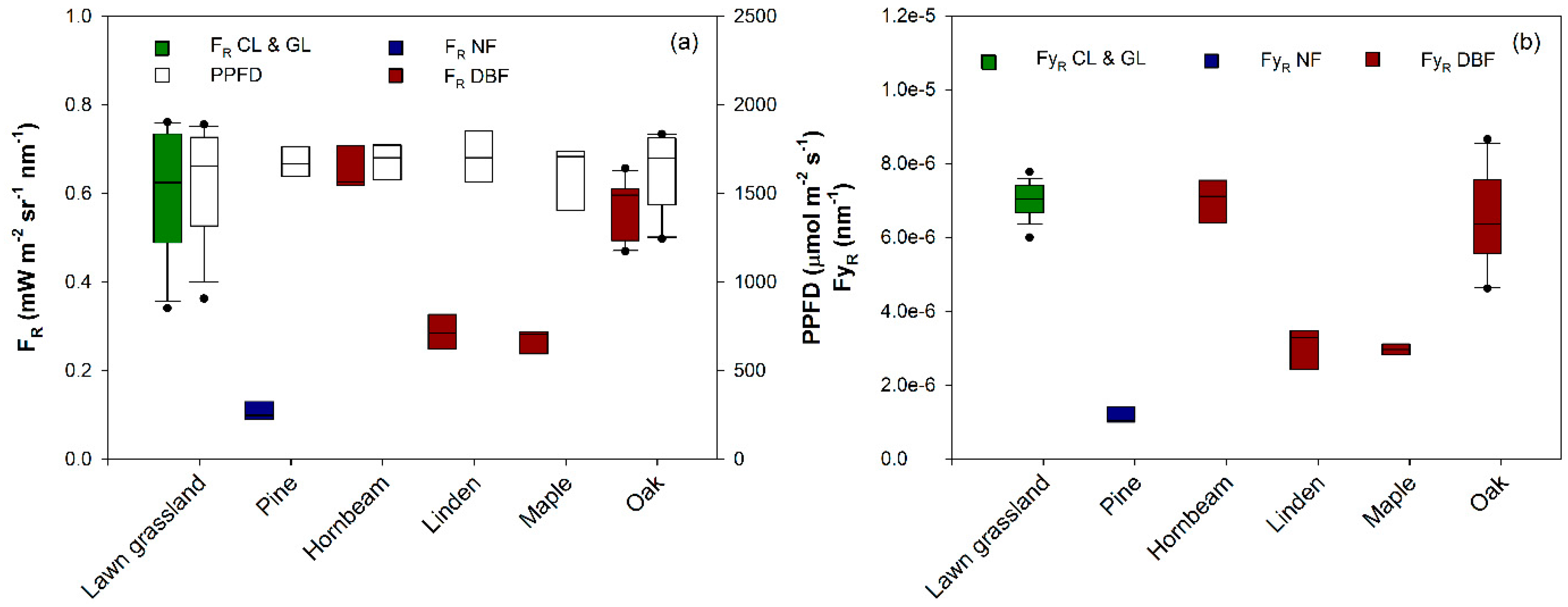
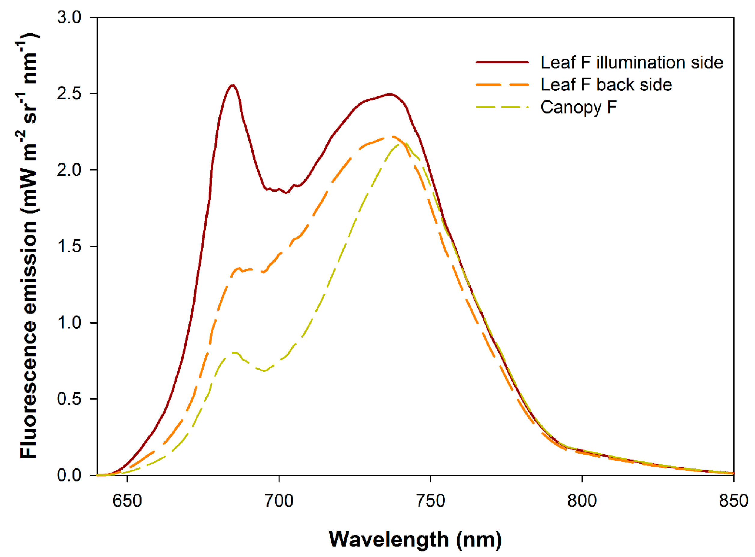
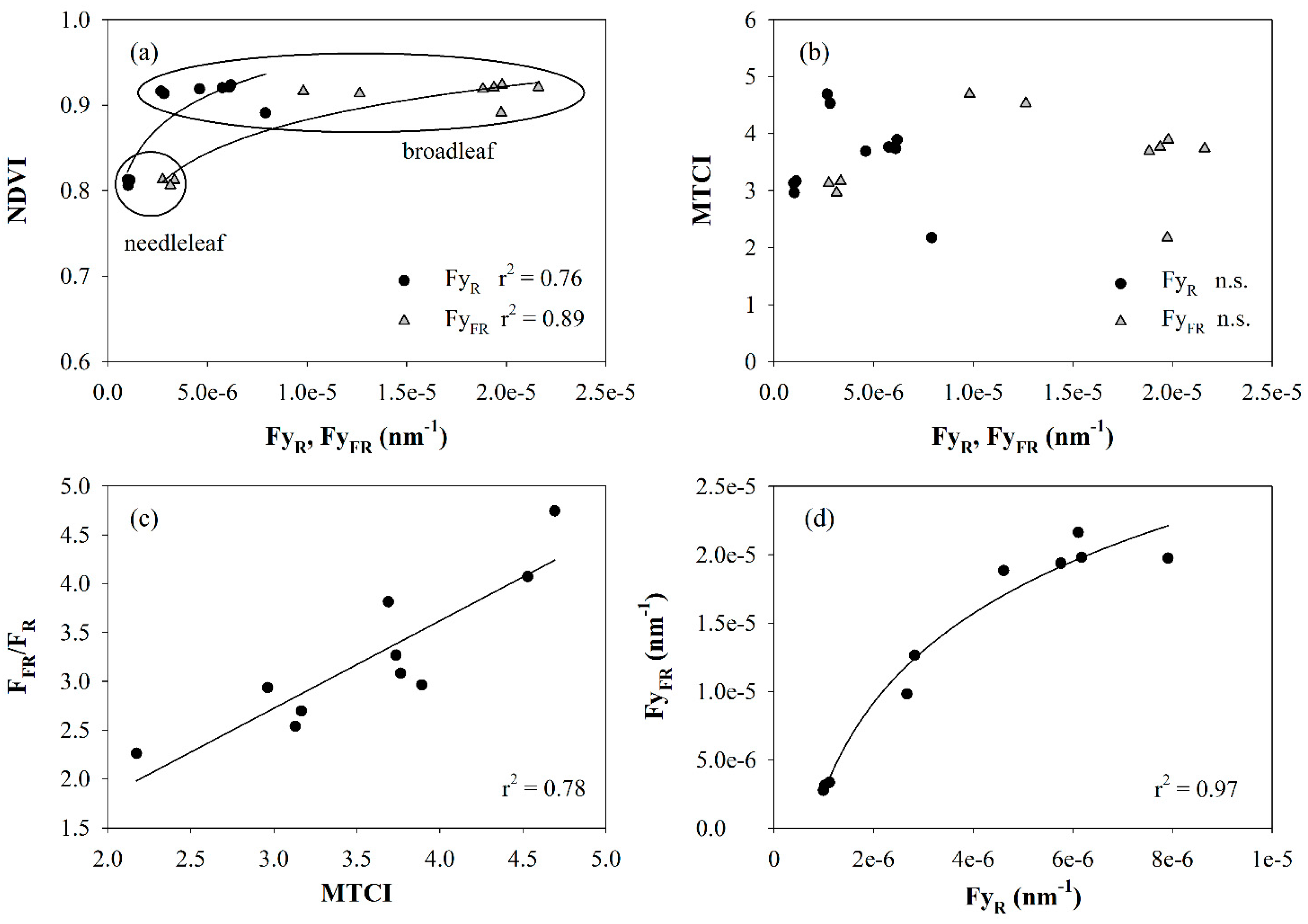
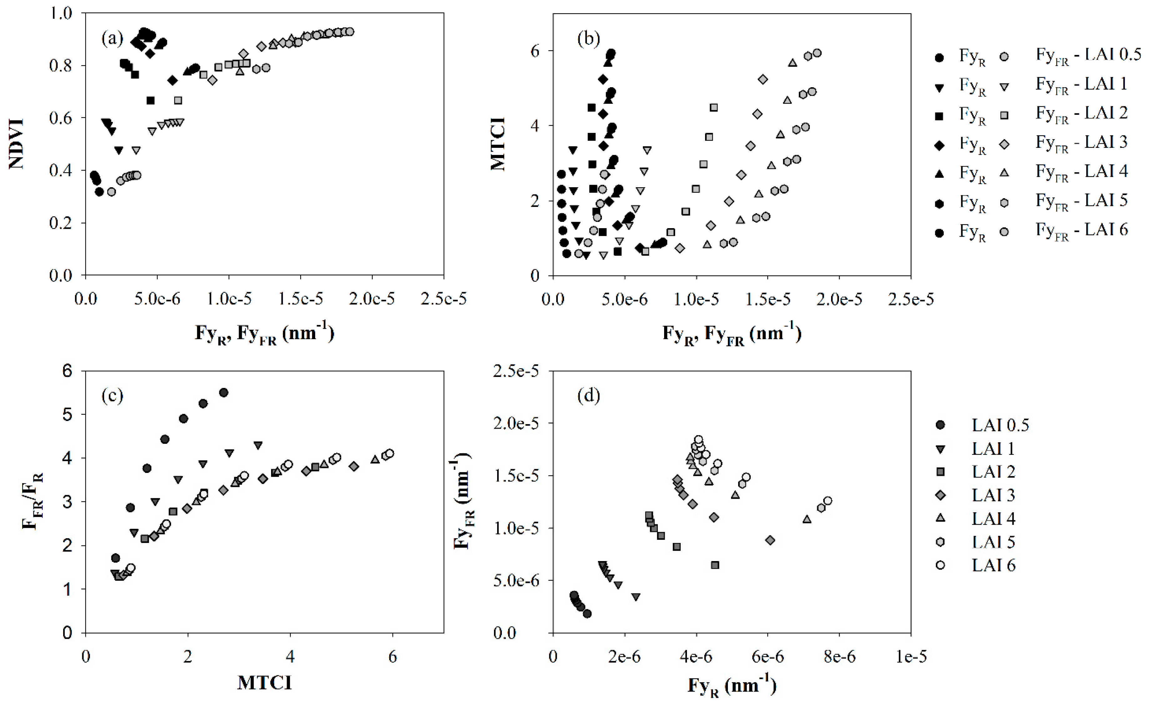
3. Results and Discussion

Sun-induced chlorophyll fluorescence measurements at the O2-A band (FFR) made under different illumination intensities varied from near 0 to 3 mW·m−2·sr−1·nm−1 in the investigated species (Figure 1a). As fluorescence emission is mainly driven by the magnitude of incident radiation, the comparison between different targets was performed by normalizing F by the incident radiation (as in Figure 1b) to get an apparent F yield (Fy). Results highlighted that different land cover classes and forest species were characterized by different FFR (Figure 1a) and FyFR (Figure 1b) values. In general, the highest emissions were measured in crops and grasslands followed by broadleaf and then needleleaf species. More in detail, maximum FFR values ranged from 0.5 mW·m−2·sr−1·nm−1 for spruce forests to 2 mW·m−2·sr−1·nm−1 for broadleaf forests and 2.5–3 mW·m−2·sr−1·nm−1 for crops for a maximum incident PPFD between 1400 and 2000 μmol·m−2·s−1. The FyFR variability within the same species is due to changes in the efficiency of fluorescence emission during a day with different irradiance loads. Lawn grassland showed the maximum FyFR among the investigated species. These findings refer to the specific dataset investigated in this study, thus they could be affected by year-to-year changes in cropland and grassland development or changes due to the specific crop species investigated. Furthermore, sun-induced chlorophyll fluorescence measurements were collected on unstressed vegetation, thus variations in fluorescence emission caused by stress conditions are not considered in this study. However, it is worth noting that they are in agreement with the patterns observed in the first FFR maps obtained from satellite platforms [9] where forests had general lower FFR values as opposed to grasslands and croplands due to the combination of complex canopy architecture and the distribution of absorbing and scattering elements determining forest canopies to act as photon traps [37,38]. In particular, coniferous trees with complex architecture, shoot level clumping and gaps had the weakest fluorescence values [3]. Similar patterns were observed in the first FFR maps obtained with the airborne high performance imaging spectrometer HyPlant developed by the Forschungszentrum Jülich and the Finnish company Specim. FFR maps showed the highest emissions in crops with dense and fully photosynthetically active canopy at the time of the overflight followed by broadleaf forests and crops approaching senescence during the time of observation [26]. As observed with ground-based data, FFR maps collected over a coniferous forest (i.e., spruce) showed the weakest FFR emission with average values close to 0.5–1 mW·m−2·sr−1·nm−1 (https://earth.esa.int/documents/10174/134665/HYFLEX_Final_Report). We cannot exclude that part of the variability in the FFR values between species is explained by different canopy biomass (i.e., LAI). However, LAI variation did not appear to be the main factor driving FFR differences between species from different plant functional types. In fact, forest species (particularly needleleaf) had generally higher LAI (Table 1) but lower FFR values than crops. This suggests that factors other than LAI were causing the observed FFR differences between plant functional types. A proper analysis of the effect of LAI variations on fluorescence values based on modeled data is reported in the paragraphs below.
Sun-induced chlorophyll fluorescence at the O2-B band (FR) was measured on a reduced number of land cover classes, mainly broadleaf and needleleaf forest species. FR and FyR values are shown in Figure 2: maximum FR values at maximum canopy development ranged from 0.1 mW·m−2·sr−1·nm−1 for pine trees to 0.8 mW·m−2·sr−1·nm−1 for broadleaf trees and grasslands with a maximum incident PPFD between 1800 and 1900 μmol·m−2·s−1 (Figure 2a). Lawn grassland and hornbeam showed the maximum FyR among the investigated species (Figure 2b).
FR values were up to four times lower than those measured in the far-red region (Figure 3). Thus, the ratio between canopy FFR and FR was considerably higher than that reported in studies performed at leaf level [39,40]. Besides the difficulties in comparing leaf and canopy measurements due to the frequent use of artificial light sources with an excitation spectrum different from the solar one for leaf studies, these higher values at canopy level can be explained considering the reabsorption of FR by photosynthetic pigments within the canopy layers causing a rise of the FFR/FR ratio compared to the leaf-level. We are aware of only two studies comparing the FFR/FR obtained at leaf and canopy level using passive technique in crops, both confirming an increase of the FFR/FR ratio from leaf to canopy. Fournier et al. [11] and Daumard et al. [39] showed that the fluorescence ratio almost doubled from leaf to canopy in velvetgrass and sorghum, respectively. To the best of our knowledge, this is the first study providing quantitative information on the magnitude of canopy sun-induced FR emission in different forest species.
The difference in the shape of the fluorescence emission spectrum at canopy scale compared to the one measured at leaf level was further characterized based on SCOPE simulations, as shown in Figure 4. Sun-induced chlorophyll fluorescence emissions at leaf level and canopy level were simulated for the grass lawn measured in [12]. When the abaxial side of a leaf is illuminated, fluorescence is emitted in both the front-side and back-side geometry in the red and far-red region of the spectrum (640–800 nm). Fluorescence emission in the front-side occurs with two peaks that have broad bands with maxima around 685 nm and 740 nm. Back-side emission occurs mostly in the far-red, as scattering is greater than absorption in this spectral region. On the contrary, chlorophyll fluorescence is strongly reabsorbed by the Chl absorption band, since the absorption of a green leaf has a maximum in the range of ca. 680 nm [41]. Very different shape of the fluorescence emission spectra at 687 nm for front-side and back-side geometry due to re-absorption of red fluorescence within the leaf was also observed by Louis et al. [42] in their work exploring the full range fluorescence excitation and emission spectra of intact leaves. The comparison between leaf illuminated side and canopy emission spectra showed an increase in FFR/FR from leaf to canopy measurements, from 0.6 to 1.8. This simulation confirms the suggestion of Van Wittenberghe et al. [40] that both multiple re-absorption in the red and scattering effects in the far-red region could cause increasing of the FFR/FR peak ratio at canopy level as compared to the leaf level.
The relationship between FyR and FyFR was further analyzed using the database collected over different broadleaf and needleleaf trees. Results showed that at canopy level both FyFR and FyR exhibited a logarithmic relationship with NDVI, suggesting that fluorescence can provide additional information in species characterized by high green biomass and leaf Chl, where NDVI tends to saturate (Figure 5a) [43]. No significant relationships were found between FyFR and FyR and MTCI (Figure 5b). Instead, MTCI was linearly related to the ratio FFR/FR with an R2 of 0.78 (Figure 5c). Re-absorption of the emitted F in the red region is responsible for the high correlation observed between FFR/FR and leaf Chl. This result was already reported at leaf level for different tree species [41,44]. FyFR generally increased with FyR, with a logarithmic relationship (R2 = 0.97) (Figure 5d) where FyFR tended to saturate for high FyR values. Although the data were best fitted by a logarithmic function, the linear model was also showing good performances with R2 equal to 0.89. Thus, additional data would be needed to increase the confidence in the hypothesized logarithmic behavior between FyFR and FyR.
Experimental observations were then compared with reflectance and fluorescence values simulated with the SCOPE model varying LAI and leaf Chl input values. Figure 6 depicts the relations between vegetation indices (i.e., NDVI and MTCI) and FyR and FyFR, as already shown with measured data (Figure 5).
As observed with ground measured data, FyFR and FyR exhibited a logarithmic relationship with NDVI (Figure 6a), suggesting that fluorescence can provide additional information compared to NDVI in vegetation characterized by a dense and green canopy. On the contrary and again in rough agreement with experimental data (Figure 5b), a general clear relationship was not identified between FyFR and FyR and MTCI (Figure 6b). This was due to the fact that the relation between FyFR and FyR and MTCI was greatly affected by LAI variations. The ratio FFR/FR exhibited a logarithmic relationship with MTCI (Figure 6c), suggesting that FFR/FR was less sensitive than MTCI to leaf Chl variations when leaf Chl was high. This result supports the hypothesis that fluorescence can provide additional information compared to traditional vegetation indices in vegetation characterized by a dense and green canopy. However, the relationship between MTCI and FFR/FR was linear in the range measured in the field, MTCI between 1.5 and 5 and LAI greater than 1 m2·m−2, confirming the good agreement between observed and modeled data. Finally, the relationship between FyFR and FyR did not show a clear behavior as instead observed with ground data (Figure 6d). For a given leaf Chl, both FyFR and FyR generally increased with LAI while for a given LAI, FyFR increased and FyR decreased with leaf Chl. It should be noted that the modeled dataset was simulated using the SCOPE model, which is a one-dimensional radiative transfer model suitable for horizontally homogeneous canopies. Thus, it has some limitations in accounting for surface heterogeneity in the horizontal direction causing effects of multiple scattering between, for example, tree crowns.
To allow a better understanding of the parameters driving the relationships shown in Figure 5 and Figure 6, influences of leaf Chl and LAI on canopy fluorescence were described by plotting simulated Fy values at 687 and 760 nm, and the FyTOT against leaf Chl for different LAI values (Figure 7). The curves depict variations in fluorescence values when leaf Chl varied from 10 to 70 mg·cm−2 with a 10 μg·cm−2 step. As expected, fluorescence was a function of both leaf Chl and LAI. The asymptotic relationship between both FyFR and FyR and leaf Chl (Figure 7a,b) suggests that Fy was insensitive to leaf Chl variations when leaf Chl was high. However, the asymptotic response to increasing leaf Chl was different for the two emission regions: FyR decreased whereas FyFR increased. Both FyFR and FyR increased as LAI increased. For high LAI values, the effect of increasing LAI was greater on FyFR than FyR. This effect was attributed to a preferential re-absorption of the FR emission compared to FFR in the optical path within the canopy. The effect of reabsorption of the FR was particularly large when leaves had a moderate to high leaf Chl content. Figure 7c displays FyTOT as a function of leaf Chl. Except for small values of leaf Chl, FyTOT was not sensitive to leaf Chl variations. The very weak sensitivity of FTOT to leaf Chl was due to the contrasting response of F emission to leaf Chl variations in the red and far-red region. However, for a given leaf Chl, the variation of FyTOT due to the LAI was significant (up to a factor of 8). The increase of the ratio FFR/FR with leaf Chl (Figure 7d) was explained by an increase of FFR with leaf Chl and a decrease of FR due to reabsorption. The relationship between FFR/FR and leaf Chl was almost insensitive to LAI variations for LAI greater than 1 m2·m−2.
In summary, we were able to explain the relationship between MTCI, leaf Chl and the fluorescence yield ratio (FyFR/FyR), and the increase of Fy with LAI with the simulation results. A closer inspection of individual land cover types, however, showed discrepancies between simulated and measured data. For example, among the broadleaf trees we found the lowest FyFR (5.8 e−6 vs. 2.2 e−5, 1.7 e−5 and 2.4 e−5·nm−1) in linden, but the lowest LAI in hornbeam (2.9 vs. 5.2, 6.2 and 6.1 m2·m−2). Similarly, the difference in FyFR between the grass and the lawn was larger than what could be expected from LAI alone. These discrepancies may be explained by: (1) differences in LAI estimates from ground measurements and from reflectance spectra; (2) the effect of other model parameters such as senescent and brown material that were not considered; and (3) effects of canopy structure such as clumping, which is not included in the model.
The comparison of simulated and measured reflectance spectra revealed differences in LAI estimates from ground measurements and from reflectance spectra (Table 3). For example, when considering the LAI computed using model inversion of acquired spectra, the linden had a lower LAI than hornbeam. In summary, plant-specific LAI retrieved with model inversion on measured spectra does not match the stand-level measured LAI (Table 3). Therefore, when the plant-specific LAI is used as a reference, the relationship between measured fluorescence and LAI is in agreement with the one described by model simulations. The observed difference between the two sets of LAI may be due to the fact that the one retrieved from model inversion matches exactly the footprint of spectral measurements and that the LAI measurements in the field may also include woody material, which absorbs but does not emit fluorescence.
The SCOPE simulations used in Figure 6 and Figure 7 were obtained using a fixed fluorescence efficiency (i.e., setting an unstressed and constant physiological status) to show that fluorescence emission was modulated by changes in leaf biochemistry and canopy density. Variations in photosynthesis (and thus fluorescence) efficiency would represent an additional driver of F emission. This implies that inference about the status of the photosynthetic machinery from F is challenging without additional information regarding the canopy LAI and leaf Chl. Simultaneous measurements of spectral reflected radiance may be used to derive such information and decompose the contribution of canopy biophysical variables and variables describing the physiological status to the F signal.
A recent study [45] showed that while leaf Chl controls FFR, it has little impact on gross primary production. This has serious implications when using FFR to constrain gross primary production estimates highlighting the need for a better treatment of leaf Chl in dynamic global vegetation models. Furthermore, the strong influence of FR re-absorption by pigments has to be taken into account when FR and or FFR are used to derive information on plant photosynthesis.
The detection of FR and FFR in combination with reflectance based estimates of pigments, could reveal changes in fluorescence due to variations of leaf Chl during plant development as well as under various stress conditions [30,46] leading to an improved understanding of plant physiological responses caused by changing environmental conditions, strain and stress events [41]. The development of strategies to decouple F modulations due to leaf Chl and LAI variations from those related to vegetation status and functioning would result in a better understanding of vegetation response to stress conditions. Fluorescence information derived from the two-peaks emission has proven to be very important in practical applications aimed at diagnosing and interpreting stress effects on vegetation status. A recent meta-analysis examined the effects of some widespread stress factors (water and nitrogen deficit, temperature extremes) on FR, FFR and FFR/FR [47]. This meta-analysis revealed that different stresses can have opposite effects on the F values as well as on FFR/FR. For example, FFR/FR increased with stress conditions caused by temperature extremes (both chilling and heat) while decreased with long-term nitrogen deficiency. However, it should be noted that, while chilling stress caused a rise of both FR and FFR values, F under nitrogen deficiency might either increase or decrease. This variable F response to nitrogen deficiency can be explained considering variations in leaf Chl caused by nitrogen deficiency, affecting FR reabsorption and consequently the FFR/FR ratio. This suggests that FR, FFR and FFR/FR bring complementary information, thus they should be collected simultaneously, when possible. Simultaneous measurements of spectral reflectance to derive information regarding leaf Chl are also beneficial for a correct interpretation of vegetation stress response.

4. Conclusions

The dataset presented in this contribution is of great importance for the characterization of fluorescence emission from different plant functional types with varying leaf and canopy characteristics, as well as the validation of the fluorescence maps derived from remote sensors with lower spatial resolution. These datasets are currently used for the validation of the maps derived from the airborne high performance imaging spectrometer HyPlant [26] acquired with a spatial resolution from 1 to 3 m pixel size and can represent a basis for the evaluation of the consistency of the fluorescence maps in the far-red region obtained from satellite platforms.
The analysis of this new dataset showed that different plant functional types and forest species were characterized by different fluorescence magnitude, in both the red and far-red region, with generally the highest fluorescence emissions in crops followed by broadleaf and then needleleaf species. FR values were up to 4 times lower than FFR. Thus the ratio between FFR and FR at canopy level was considerably higher than that measured so far on single leaves. These higher values at canopy level can be explained considering the reabsorption of FR by photosynthetic pigments within the canopy layers. Simulations performed with the SCOPE model agreed with experimental data and confirmed that this behavior can be successfully reproduced by SCOPE version 1.61.
The analysis of the measured data supported by the simulations performed with the SCOPE model showed that canopy chlorophyll fluorescence depended on the variation of leaf characteristics, particularly leaf chlorophyll concentration, as well as vegetation density as expressed by LAI. However, some discrepancies between simulated and measured data were observed for broadleaf species. These discrepancies were most likely explained by differences in LAI estimates from ground measurements and from reflectance spectra, even if we cannot exclude the effect of other model parameters and/or model representation errors.
Overall, the results gathered in this study highlight the need to decouple F modulations due to leaf Chl and LAI variations from those related to vegetation status. This is the concept behind the ESA FLEX satellite mission recently selected as the 8th Earth Explorer mission. This satellite will be equipped with a sensor spanning the red and far-red spectral regions with a subnanometric spectral resolution, allowing the retrieval of both FR and FFR at an unparalleled spatial resolution of 300 m and biweekly repeat coverage. FLEX will fly in tandem with SENTINEL 3 enabling improved retrievals, not only of sun-induced fluorescence, but also of complementary biophysical variables such as LAI and leaf chlorophyll content.

Acknowledgments

We gratefully acknowledge the financial support by the European Space Agency (ESA) within the framework of the “Sen2Exp, Technical Assistance to fieldwork in the Harth forest during SEN2Exp” project (ESA contract 4000110267/14/NL/BJ/lf). We thank four anonymous reviewers for valuable comments on the paper.

Author Contributions

Micol Rossini conceived the study, organized data analysis and wrote the paper with discussions and contributions from all co-authors. Michele Meroni, Marco Celesti, Sergio Cogliati, Tommaso Julitta, Cinzia Panigada and Roberto Colombo performed the ground measurements and contributed to data analysis. Michele Meroni and Sergio Cogliati developed the processing pipeline for fluorescence retrieval. Uwe Rascher helped to interpret the physiological results. Christiaan van der Tol provided the model SCOPE and contributed to interpretation of the modeling results.

Conflicts of Interest

The authors declare no conflict of interest.

References

  1. Porcar-Castell, A.; Tyystjärvi, E.; Atherton, J.; van der Tol, C.; Flexas, J.; Pfündel, E.E.; Moreno, J.; Frankenberg, C.; Berry, J.A. Linking chlorophyll a fluorescence to photosynthesis for remote sensing applications: Mechanisms and challenges. J. Exp. Bot. 2014, 65, 4065–4095. [Google Scholar] [CrossRef] [PubMed]
  2. Meroni, M.; Rossini, M.; Guanter, L.; Alonso, L.; Rascher, U.; Colombo, R.; Moreno, J. Remote sensing of solar-induced chlorophyll fluorescence: Review of methods and applications. Remote Sens. Environ. 2009, 113, 2037–2051. [Google Scholar] [CrossRef]
  3. Frankenberg, C.; Fisher, J.B.; Worden, J.; Badgley, G.; Saatchi, S.S.; Lee, J.-E.; Toon, G.C.; Butz, A.; Jung, M.; Kuze, A.; et al. New global observations of the terrestrial carbon cycle from gosat: Patterns of plant fluorescence with gross primary productivity. Geophys. Res. Lett. 2011, 38. [Google Scholar] [CrossRef]
  4. Guanter, L.; Frankenberg, C.; Dudhia, A.; Lewis, P.E.; Gómez-Dans, J.; Kuze, A.; Suto, H.; Grainger, R.G. Retrieval and global assessment of terrestrial chlorophyll fluorescence from gosat space measurements. Remote Sens. Environ. 2012, 121, 236–251. [Google Scholar] [CrossRef]
  5. Joiner, J.; Guanter, L.; Lindstrot, R.; Voigt, M.; Vasilkov, A.P.; Middleton, E.M.; Huemmrich, K.F.; Yoshida, Y.; Frankenberg, C. Global monitoring of terrestrial chlorophyll fluorescence from moderate-spectral-resolution near-infrared satellite measurements: Methodology, simulations, and application to GOME-2. Atmos. Meas. Tech. 2013, 6, 2803–2823. [Google Scholar] [CrossRef]
  6. Frankenberg, C.; O’Dell, C.; Berry, J.; Guanter, L.; Joiner, J.; Köhler, P.; Pollock, R.; Taylor, T.E. Prospects for chlorophyll fluorescence remote sensing from the orbiting carbon observatory-2. Remote Sens. Environ. 2014, 147, 1–12. [Google Scholar] [CrossRef]
  7. Perez-Priego, O.; Guan, J.; Rossini, M.; Fava, F.; Wutzler, T.; Moreno, G.; Carvalhais, N.; Carrara, A.; Kolle, O.; Julitta, T.; et al. Sun-induced chlorophyll fluorescence and photochemical reflectance index improve remote-sensing gross primary production estimates under varying nutrient availability in a typical mediterranean savanna ecosystem. Biogeosciences 2015, 12, 6351–6367. [Google Scholar] [CrossRef]
  8. Guanter, L.; Rossini, M.; Colombo, R.; Meroni, M.; Frankenberg, C.; Lee, J.-E.; Joiner, J. Using field spectroscopy to assess the potential of statistical approaches for the retrieval of sun-induced chlorophyll fluorescence from ground and space. Remote Sens. Environ. 2013, 133, 52–61. [Google Scholar] [CrossRef]
  9. Guanter, L.; Zhang, Y.; Jung, M.; Joiner, J.; Voigt, M.; Berry, J.A.; Frankenberg, C.; Huete, A.R.; Zarco-Tejada, P.; Lee, J.-E.; et al. Global and time-resolved monitoring of crop photosynthesis with chlorophyll fluorescence. Proc. Natl. Acad. Sci. USA 2014, 111, E1327–E1333. [Google Scholar] [CrossRef] [PubMed]
  10. Yang, X.; Tang, J.; Mustard, J.F.; Lee, J.-E.; Rossini, M.; Joiner, J.; Munger, J.W.; Kornfeld, A.; Richardson, A.D. Solar-induced chlorophyll fluorescence that correlates with canopy photosynthesis on diurnal and seasonal scales in a temperate deciduous forest. Geophys. Res. Lett. 2015, 42, 2977–2987. [Google Scholar] [CrossRef]
  11. Fournier, A.; Daumard, F.; Champagne, S.; Ounis, A.; Goulas, Y.; Moya, I. Effect of canopy structure on sun-induced chlorophyll fluorescence. ISPRS J. Photogramm. Remote Sens. 2012, 68, 112–120. [Google Scholar] [CrossRef]
  12. Rossini, M.; Nedbal, L.; Guanter, L.; Ač, A.; Alonso, L.; Burkart, A.; Cogliati, S.; Colombo, R.; Damm, A.; Drusch, M.; et al. Red and far-red sun-induced chlorophyll fluorescence as a measure of plant photosynthesis. Geophys. Res. Lett. 2015, 42, 1632–1639. [Google Scholar] [CrossRef]
  13. Verrelst, J.; Rivera, J.P.; van der Tol, C.; Magnani, F.; Mohammed, G.; Moreno, J. Global sensitivity analysis of the scope model: What drives simulated canopy-leaving sun-induced fluorescence? Remote Sens. Environ. 2015, 166, 8–21. [Google Scholar] [CrossRef]
  14. Julitta, T.; Corp, L.; Rossini, M.; Burkart, A.; Cogliati, S.; Davies, N.; Hom, M.; MacArthur, A.; Middleton, E.; Rascher, U.; et al. Comparison of sun-induced chlorophyll fluorescence estimates obtained from four portable field spectroradiometers. Remote Sens. 2015, 8, 122. [Google Scholar] [CrossRef]
  15. Damm, A.; Erler, A.; Hillen, W.; Meroni, M.; Schaepman, M.E.; Verhoef, W.; Rascher, U. Modeling the impact of spectral sensor configurations on the fld retrieval accuracy of sun-induced chlorophyll fluorescence. Remote Sens. Environ. 2011, 115, 1882–1892. [Google Scholar] [CrossRef]
  16. Alonso, L.; Gomez-Chova, L.; Vila-Frances, J.; Amoros-Lopez, J.; Guanter, L.; Calpe, J.; Moreno, J. Improved fraunhofer line discrimination method for vegetation fluorescence quantification. IEEE Geosci. Remote Sens. Lett. 2008, 5, 620–624. [Google Scholar] [CrossRef]
  17. Meroni, M.; Busetto, L.; Colombo, R.; Guanter, L.; Moreno, J.; Verhoef, W. Performance of spectral fitting methods for vegetation fluorescence quantification. Remote Sens. Environ. 2010, 114, 363–374. [Google Scholar] [CrossRef]
  18. Van der Tol, C.; Verhoef, W.; Timmermans, J.; Verhoef, A.; Su, Z. An integrated model of soil-canopy spectral radiances, photosynthesis, fluorescence, temperature and energy balance. Biogeosciences 2009, 6, 3109–3129. [Google Scholar] [CrossRef]
  19. Rouse, J.W.; Haas, R.H.; Schell, J.A.; Deering, D.W.; Harlan, J.C. Monitoring the Vernal Advancements and Retro Gradation of Natural Vegetation; NASA/GSFC: Greenbelt, MD, USA, 1974; p. 371.
  20. Dash, J.; Curran, P.J. The meris terrestrial chlorophyll index. Int. J. Remote Sens. 2004, 25, 5403–5413. [Google Scholar] [CrossRef]
  21. Meroni, M.; Colombo, R. Leaf level detection of solar induced chlorophyll fluorescence by means of a subnanometer resolution spectroradiometer. Remote Sens. Environ. 2006, 103, 438–448. [Google Scholar] [CrossRef]
  22. Cogliati, S.; Verhoef, W.; Kraft, S.; Sabater, N.; Alonso, L.; Vicent, J.; Moreno, J.; Drusch, M.; Colombo, R. Retrieval of sun-induced fluorescence using advanced spectral fitting methods. Remote Sens. Environ. 2015, 169, 344–357. [Google Scholar] [CrossRef]
  23. Gilmanov, T.G.; Tieszen, L.L.; Wylie, B.K.; Flanagan, L.B.; Frank, A.B.; Haferkamp, M.R.; Meyers, T.P.; Morgan, J.A. Integration of CO2 flux and remotely-sensed data for primary production and ecosystem respiration analyses in the northern great plains: Potential for quantitative spatial extrapolation. Glob. Ecol. Biogeogr. 2005, 14, 271–292. [Google Scholar] [CrossRef]
  24. Rossini, M.; Meroni, M.; Migliavacca, M.; Manca, G.; Cogliati, S.; Busetto, L.; Picchi, V.; Cescatti, A.; Seufert, G.; Colombo, R. High resolution field spectroscopy measurements for estimating gross ecosystem production in a rice field. Agric. For. Meteorol. 2010, 150, 1283–1296. [Google Scholar] [CrossRef]
  25. Cogliati, S.; Colombo, R.; Rossini, M.; Meroni, M.; Julitta, T.; Panigada, C. Retrieval of vegetation fluorescence from ground-based and airborne high resolution measurements. In Proceedings of the 2002 IEEE International Geoscience and Remote Sensing Symposium (IGARSS), Munich, Germany, 22–27 July 2012; pp. 7129–7132.
  26. Rascher, U.; Alonso, L.; Burkart, A.; Cilia, C.; Cogliati, S.; Colombo, R.; Damm, A.; Drusch, M.; Guanter, L.; Hanus, J.; et al. Sun-induced fluorescence—A new probe of photosynthesis: First maps from the imaging spectrometer hyplant. Glob. Chang. Biol. 2015, 21, 4673–4684. [Google Scholar] [CrossRef] [PubMed]
  27. Cogliati, S.; Rossini, M.; Julitta, T.; Meroni, M.; Schickling, A.; Burkart, A.; Pinto, F.; Rascher, U.; Colombo, R. Continuous and long-term measurements of reflectance and sun-induced chlorophyll fluorescence by using novel automated field spectroscopy systems. Remote Sens. Environ. 2015, 164, 270–281. [Google Scholar] [CrossRef]
  28. Meroni, M.; Barducci, A.; Cogliati, S.; Castagnoli, F.; Rossini, M.; Busetto, L.; Migliavacca, M.; Cremonese, E.; Galvagno, M.; Colombo, R.; et al. The hyperspectral irradiometer, a new instrument for long-term and unattended field spectroscopy measurements. Rev. Sci. Instrum. 2011, 82, 043106. [Google Scholar] [CrossRef] [PubMed]
  29. Lichtenthaler, H.K.; Buschmann, C. Chlorophylls and carotenoids: Measurement and characterization by UV-VIS spectroscopy. In Current Protocols in Food Analytical Chemistry; John Wiley & Sons, Inc.: Hoboken, NJ, USA, 2001. [Google Scholar]
  30. Panigada, C.; Rossini, M.; Busetto, L.; Meroni, M.; Fava, F.; Colombo, R. Chlorophyll concentration mapping with MIVIS data to assess crown discoloration in the Ticino Park oak forest. Int. J. Remote Sens. 2010, 31, 3307–3332. [Google Scholar] [CrossRef]
  31. Verhoef, W. Light scattering by leaf layers with application to canopy reflectance modeling: The sail model. Remote Sens. Environ. 1984, 16, 125–141. [Google Scholar] [CrossRef]
  32. Verrelst, J.; van der Tol, C.; Magnani, F.; Sabater, N.; Rivera, J.P.; Mohammed, G.; Moreno, J. Evaluating the predictive power of sun-induced chlorophyll fluorescence to estimate net photosynthesis of vegetation canopies: A scope modeling study. Remote Sens. Environ. 2016, 176, 139–151. [Google Scholar] [CrossRef]
  33. Verhoef, W. Modeling vegetation fluorescence observations. In Proceedings of the EARSel 7th SIG-Imaging Spectroscopy Workshop, Edinburgh, UK, 11–13 April 2011.
  34. Jacquemoud, S.; Baret, F. Prospect—A model of leaf optical-properties spectra. Remote Sens. Environ. 1990, 34, 75–91. [Google Scholar] [CrossRef]
  35. Van der Tol, C.; Berry, J.A.; Campbell, P.K.E.; Rascher, U. Models of fluorescence and photosynthesis for interpreting measurements of solar-induced chlorophyll fluorescence. J. Geophys. Res. Biogeosci. 2014, 119, 2312–2327. [Google Scholar] [CrossRef]
  36. Verhoef, W.; Jia, L.; Qing, X.; Su, Z. Unified optical-thermal four-stream radiative transfer theory for homogeneous vegetation canopies. IEEE Trans. Geosci. Remote Sens. 2007, 45, 1808–1822. [Google Scholar] [CrossRef]
  37. Knyazikhin, Y.; Schull, M.A.; Stenberg, P.; Mõttus, M.; Rautiainen, M.; Yang, Y.; Marshak, A.; Latorre Carmona, P.; Kaufmann, R.K.; Lewis, P.; et al. Hyperspectral remote sensing of foliar nitrogen content. Proc. Natl. Acad. Sci. USA 2013, 110, E185–E192. [Google Scholar] [CrossRef] [PubMed]
  38. Lewis, P.; Disney, M. Spectral invariants and scattering across multiple scales from within-leaf to canopy. Remote Sens. Environ. 2007, 109, 196–206. [Google Scholar] [CrossRef]
  39. Daumard, F.; Goulas, Y.; Champagne, S.; Fournier, A.; Ounis, A.; Olioso, A.; Moya, I. Continuous monitoring of canopy level sun-induced chlorophyll fluorescence during the growth of a sorghum field. IEEE Trans. Geosci. Remote Sens. 2012, 50, 4292–4300. [Google Scholar] [CrossRef]
  40. Van Wittenberghe, S.; Alonso, L.; Verrelst, J.; Moreno, J.; Samson, R. Bidirectional sun-induced chlorophyll fluorescence emission is influenced by leaf structure and light scattering properties—A bottom-up approach. Remote Sens. Environ. 2015, 158, 169–179. [Google Scholar] [CrossRef]
  41. Buschmann, C. Variability and application of the chlorophyll fluorescence emission ratio red/far-red of leaves. Photosynth. Res. 2007, 92, 261–271. [Google Scholar] [CrossRef] [PubMed]
  42. Louis, J.; Cerovic, Z.G.; Moya, I.L. Quantitative study of fluorescence excitation and emission spectra of bean leaves. J. Photochem. Photobiol. B Biol. 2006, 85, 65–71. [Google Scholar] [CrossRef] [PubMed]
  43. Rascher, U.; Agati, G.; Alonso, L.; Cecchi, G.; Champagne, S.; Colombo, R.; Damm, A.; Daumard, F.; de Miguel, E.; Fernandez, G.; et al. Cefles2: The remote sensing component to quantify photosynthetic efficiency from the leaf to the region by measuring sun-induced fluorescence in the oxygen absorption bands. Biogeosciences 2009, 6, 1181–1198. [Google Scholar] [CrossRef] [Green Version]
  44. Gitelson, A.A.; Buschmann, C.; Lichtenthaler, H.K. Leaf chlorophyll fluorescence corrected for re-absorption by means of absorption and reflectance measurements. J. Plant Physiol. 1998, 152, 283–296. [Google Scholar] [CrossRef]
  45. Koffi, E.N.; Rayner, P.J.; Norton, A.J.; Frankenberg, C.; Scholze, M. Investigating the usefulness of satellite-derived fluorescence data in inferring gross primary productivity within the carbon cycle data assimilation system. Biogeosciences 2015, 12, 4067–4084. [Google Scholar] [CrossRef]
  46. Rossini, M.; Panigada, C.; Meroni, M.; Colombo, R. Assessment of oak forest condition based on leaf biochemical variables and chlorophyll fluorescence. Tree Physiol. 2006, 26, 1487–1496. [Google Scholar] [CrossRef] [PubMed]
  47. Ač, A.; Malenovsky, Z.; Olejníčková, J.; Gallé, A.; Rascher, U.; Mohammed, G. Meta-analysis assessing potential of steady-state chlorophyll fluorescence for remote sensing detection of plant water, temperature and nitrogen stress. Remote Sens. Environ. 2015, 168, 420–436. [Google Scholar] [CrossRef]
Figure 1. (a) Plot of the median, 10th, 25th, 75th and 90th percentiles as vertical boxes of the F; and (b) apparent fluorescence yield in the O2-A band for different species. Full bars refer to F and Fy estimation, while empty bars refer to the incident photosynthetic photon flux density (PPFD) expressed in μmol·m−2·s−1. The statistics refer to 20 samples for each species. CL: cropland, GL: grassland, NF: Needleleaf Forest, DBF: Deciduous Broadleaf Forest.
Remotesensing 08 00412 g001
Figure 2. (a) Plot of the median, 10th, 25th, 75th and 90th percentiles as vertical boxes of the F; and (b) apparent fluorescence yield in the O2-B band for different species. Full bars refer to F and Fy estimation, while empty bars refer to the incident photosynthetic photon flux density (PPFD) expressed in μmol·m−2·s−1. The statistics refer to 20 samples for each species. CL: cropland, GL: grassland, NF: Needleleaf Forest, DBF: Deciduous Broadleaf Forest.
Remotesensing 08 00412 g002
Figure 3. Plot of the median, 10th, 25th, 75th and 90th percentiles as vertical boxes of the ratio between FFR and FR estimated at canopy level (full bars). Empty bars refer to the incident photosynthetic photon flux density (PPFD) expressed in μmol·m−2·s−1. The statistics refer to 20 samples for each species. CL: cropland, GL: grassland, NF: Needleleaf Forest, DBF: Deciduous Broadleaf Forest.
Remotesensing 08 00412 g003
Figure 4. Spectral shapes of fluorescence emission at the leaf level in the illumination and back-side and at the canopy level for a nadir observation simulated with the SCOPE model. The grass leaf emission spectrum was simulated with the following inputs: leaf chlorophyll concentration of 29 µg·cm−2, equivalent water thickness of 0.00207 cm, dry matter content of 0.001 g·cm−2, senescent material of 0.148, leaf structure parameter N of 1.5. Simulated leaf is perpendicular to the solar beam. The canopy spectrum has been simulated for the control grass reported in [12] at noon with a Leaf Area Index of 4.3 m2·m−2.
Remotesensing 08 00412 g004
Figure 5. Measured data. Relationships between: (a) FyR, FyFR and NDVI; (b) FyR, FyFR and MTCI; (c) FFR/FR ratio and MTCI; and (d) FyR and FyFR. Each point indicates the half-hourly average value measured between 11:00 a.m. and 1:00 p.m. local solar time.
Remotesensing 08 00412 g005
Figure 6. Simulated data. Relationships between: (a) FyR, FyFR and NDVI; (b) FyR, FyFR and MTCI; (c) FFR/FR ratio and MTCI; and (d) FyR and FyFR computed from the SCOPE simulations.
Remotesensing 08 00412 g006
Figure 7. Simulated data. Relationships between the leaf chlorophyll concentration (μg·cm−2) and: (a) FyR (nm−1); (b) FyFR (nm−1); (c) FyTOT; and (d) the FFR/FR ratio. Fy is derived from SCOPE simulations for different LAI values. Values for incoming shortwave radiation were set to 1000 W·m−2.
Remotesensing 08 00412 g007
Table 1. List of the investigated species, plant functional types (CL: cropland, GL: grassland, NF: Needleleaf Forest, DBF: Deciduous Broadleaf Forest), day of measurements and the spectral range investigated: VIS-NIR refers to the visible-near infrared spectral region from 400 to 1000 nm, FR refers to the spectral region around the O2-B band (657–740 nm) and FFR refers to the spectral region around the O2-A band (700–800 nm). Leaf Area Index (m2·m−2) is also reported when available. n.a. is not available. The symbol × denotes the availability of the measurement.
SpeciesPlant Functional TypeDay of MeasurementVIS-NIRFRFFRLeaf Area Index (m2·m−2)Refs.
Rice (Oryza sativa L.)CL18 July 2007×n.a.×3.7[24]
Sorghum (Sorghum bicolor L.)CL9 July 2008×n.a.×2.8n.a.
Corn (Zea mays L.)CL19 July 2010×n.a.×2.9[25]
Sugar beet (Beta Vulgaris L.)CL23 August 2012×n.a.×4.0[26]
Alfalfa (Medicago sativa L.)CL18 July 2009×n.a.×n.a.[27]
Grassland (Nardus stricta, Arnica montana, Trifolium alpinum, and Carex sempervirens as dominant species)GL28 July 2009×n.a.×2.9[28]
Lawn grassland (Festuca rubra, Lolium perenne, and Poa pratensis)GL9 September 2012×××4.3[12]
Norway spruce (Picea abies (L.) Karst)NF9 September 2012×n.a.×8.0n.a.
Pine (Pinus L.)NF17 June 2013×××4.2n.a.
Hornbeam (Carpinus betulus L.)DBF16 June 2013×××2.9n.a.
Linden (Tilia L.)DBF2 July 2013×××5.2n.a.
Maple (Acer platanoide L.)DBF17 June 2013×××6.2n.a.
Oak (Quercus robur L.)DBF16 June 2013×××5.1n.a.
Table 2. Average and standard deviation of leaf chlorophyll concentration (μg·cm−2) extracted for Hornbeam (Carpinus betulus L.), Linden (Tilia L.), Maple (Acer platanoide L.) and Oak (Quercus robur L.).
SpeciesAverage Leaf Chl (μg·cm−2)Standard Deviation Leaf Chl (μg·cm−2)
Hornbeam (Carpinus betulus L.)27.95.5
Linden (Tilia L.)50.75.1
Maple (Acer platanoide L.)55.74.1
Oak (Quercus robur L.)41.38.5
Table 3. Modeled and measured LAI and leaf chlorophyll concentration (μg·cm−2) for Hornbeam (Carpinus betulus L.), Linden (Tilia L.), Maple (Acer platanoide L.) and Oak (Quercus robur L.).
SpeciesLAI Mod (m2·m−2)Leaf Chl Mod (μg·cm−2)LAI Meas (m2·m−2)Leaf Chl Meas (μg·cm−2)
Hornbeam (Carpinus betulus L.)4.326.02.927.9
Linden (Tilia L.)3.650.75.250.7
Maple (Acer platanoide L.)2.860.96.255.7
Oak (Quercus robur L.)4.340.75.141.3
Table 4. The most relevant parameters used for the SCOPE simulations for a C3 canopy. Parameters Cdm, Cs, Cw, Cca, and N are PROSPECT parameters [34], and refer to dry matter content, senescent material, water content, carotenoid concentration and leaf structure, respectively. LIDFa and LIDFb are leaf angle distribution parameters [36]. The values in the table refer to a spherical distribution of leaves. Vcmax is the maximum carboxylation rate. The solar zenith and azimuth angles and observer zenith angle are also reported.
ParameterValueUnit
Cdm0.012g·cm−2
Cs0
Cw0.009cm
Cca20µg·cm−2
N1.4
LIDFa−0.35
LIDFb−0.15
Vcmax30µmol·m−2·s−1
Solar zenith angle30deg
Solar azimuth angle90deg
Observer zenith angle0deg

