
Retrieving Precipitable Water Vapor Data Using GPS Zenith Delays and Global Reanalysis Data in China

Abstract
:
1. Introduction
2. Methodology
2.1. GPS PWV Estimation
2.2. Interpolation of NCEP FNL Global Analysis Data
3. Interpolation Results
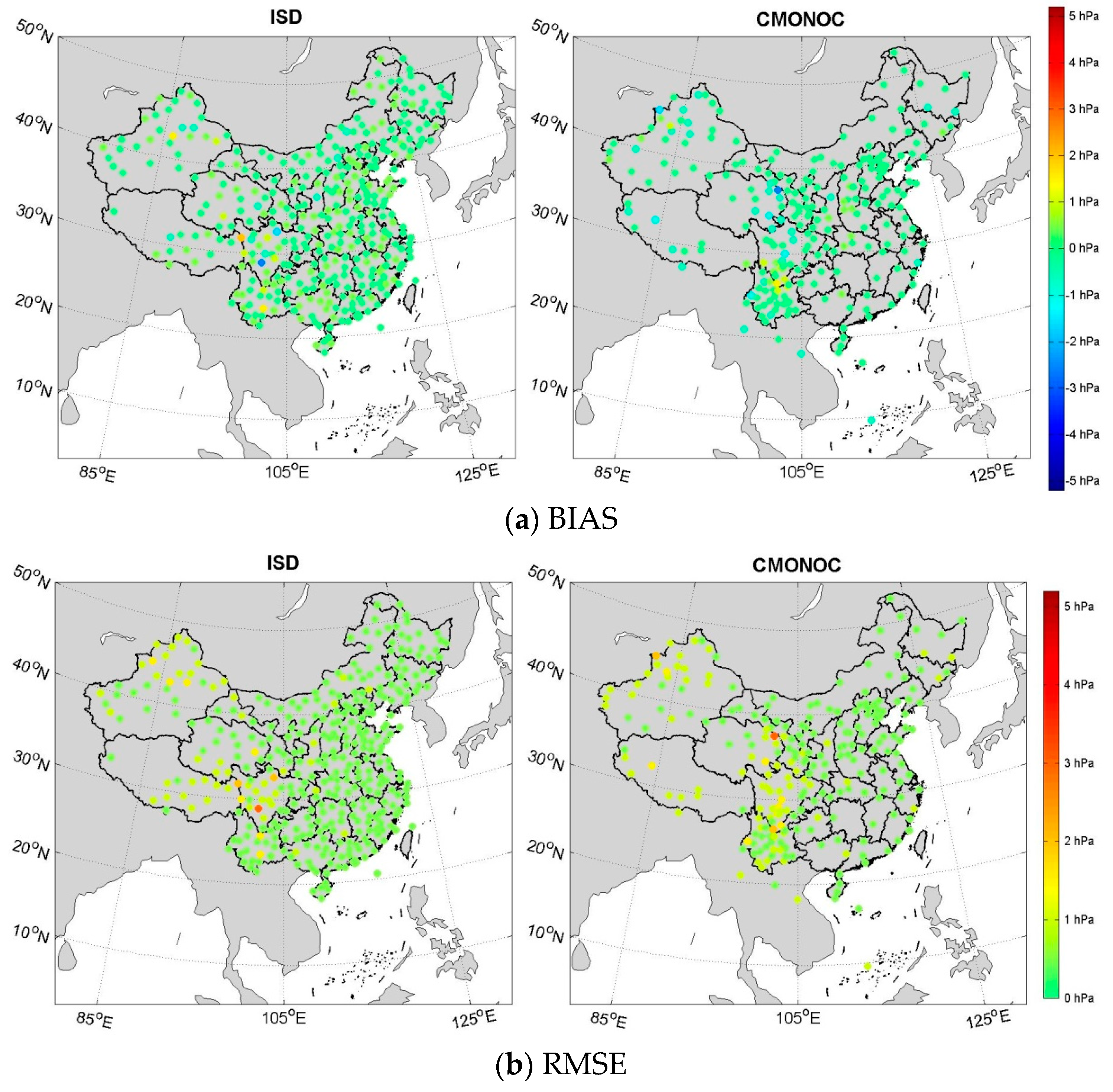
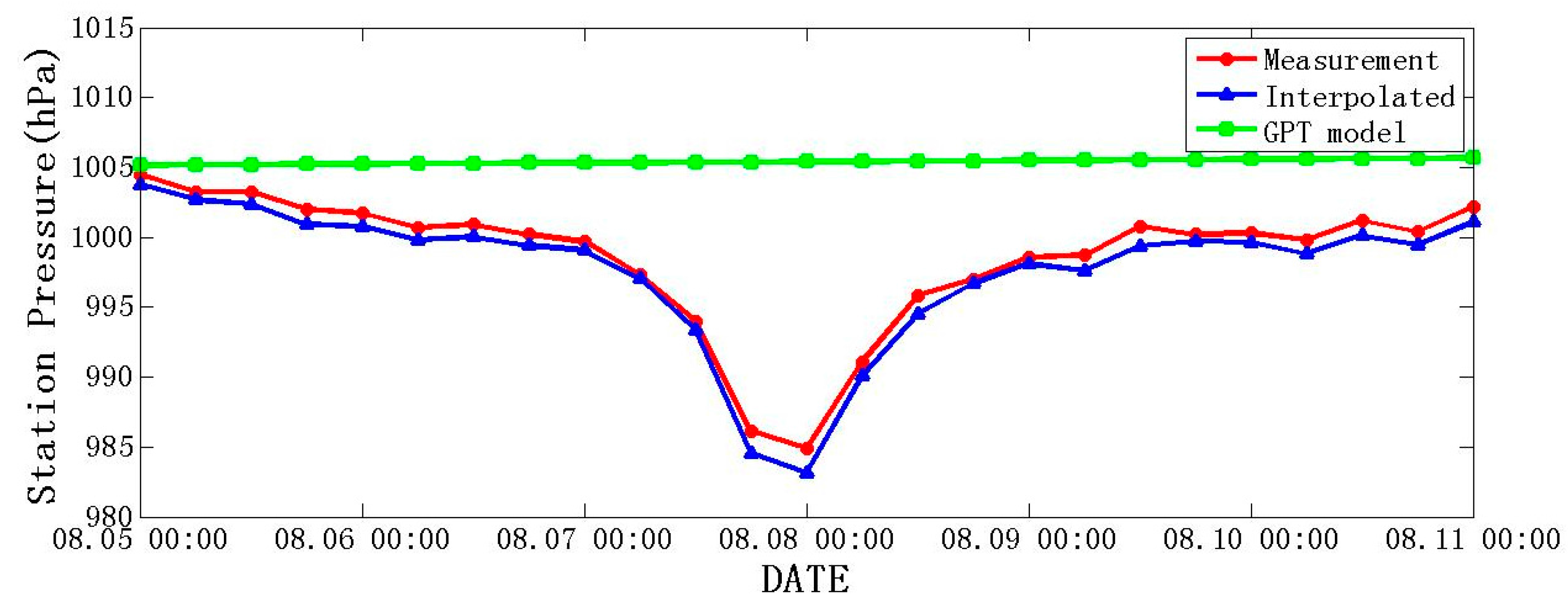
3.1. Comparison between Interpolated and Observed Ps
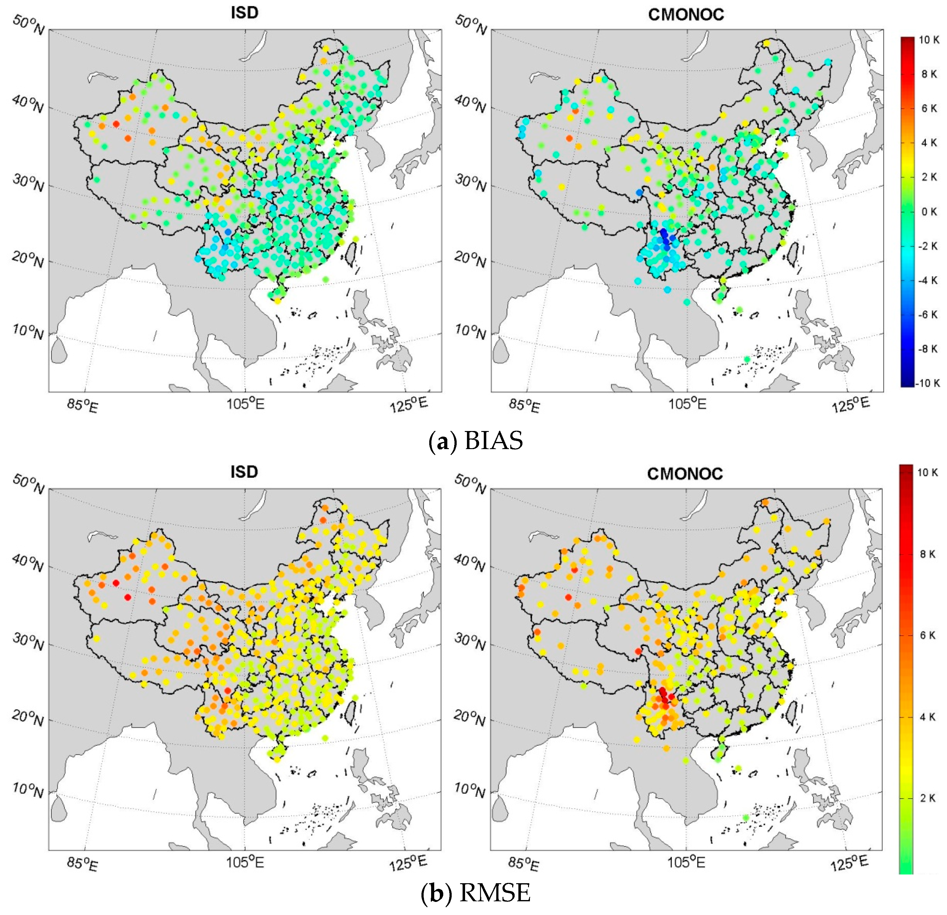
3.2. Comparison between Interpolated and Observed Ts
4. Comparison of PWV Results
4.1. Results of Different Tm
- (1)
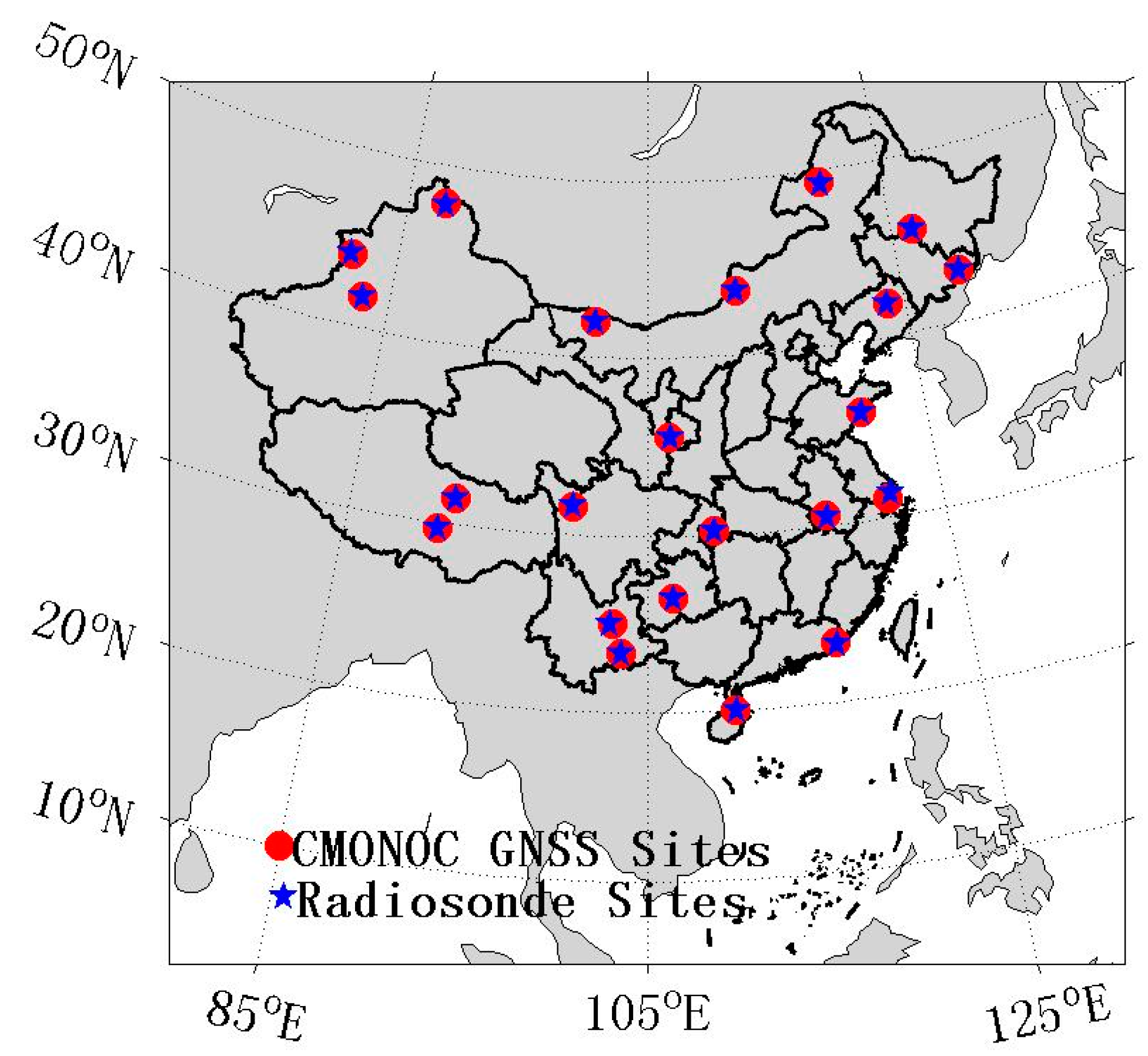
- At all of the RS stations, we directly integrated the radiosonde data assuming that the balloon ascended along a vertical path. The following approximate formula is used:where water vapor pressure e is calculated by e = es ×RH, RH represents the relative humidity, and saturation vapor pressure is generated using ITS-90 equations proposed by [37]. We denoted Tm by this method as Tm_RS.
- (2)
- At selected CMONOC stations in Table 3, Tm was estimated from Ts using the Tm–Ts linear equation of Equation (7). From Wang’s research [38], coefficients a and b are determined by the climatic region of every site. Ts was measured by the meteorological sensors collocated to the CMONOC GNSS sites. Then, Tm_OW could be obtained.
- (3)
- The same method as in Equation (2) was employed, except that Ts was obtained from the interpolation schemes described in Section 2. To differentiate their results, we denoted the results from this method as Tm_IW.
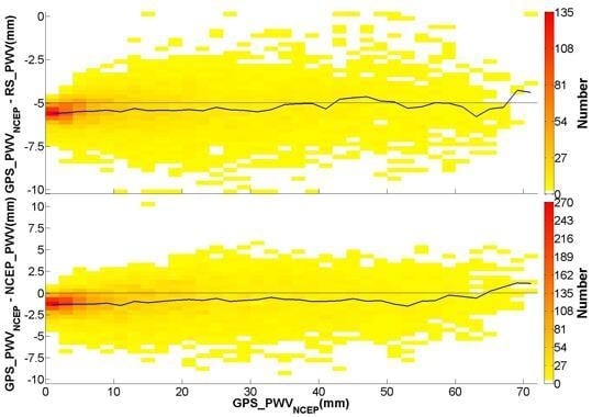
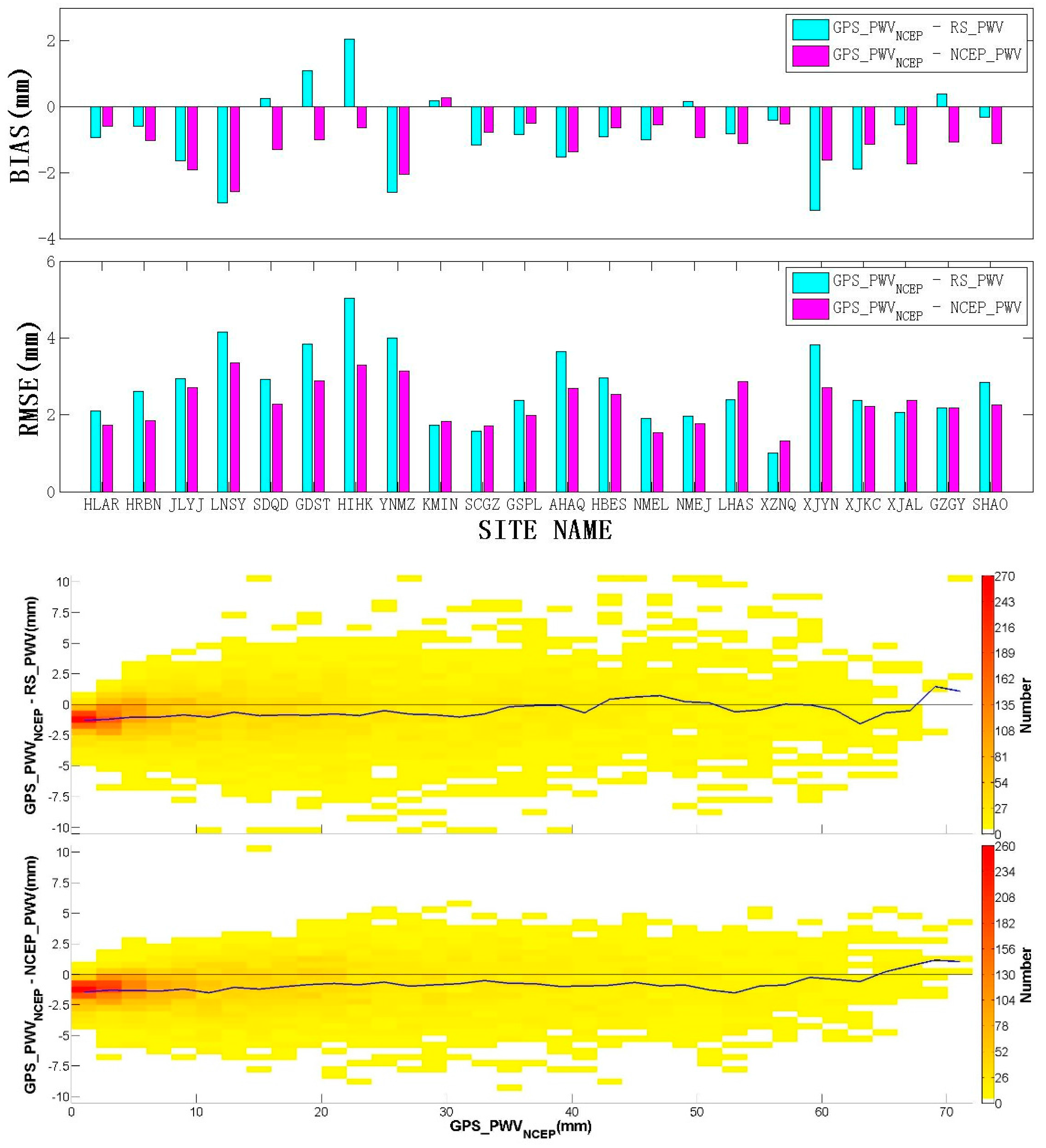
4.2. Results of Different PWV
- (1)
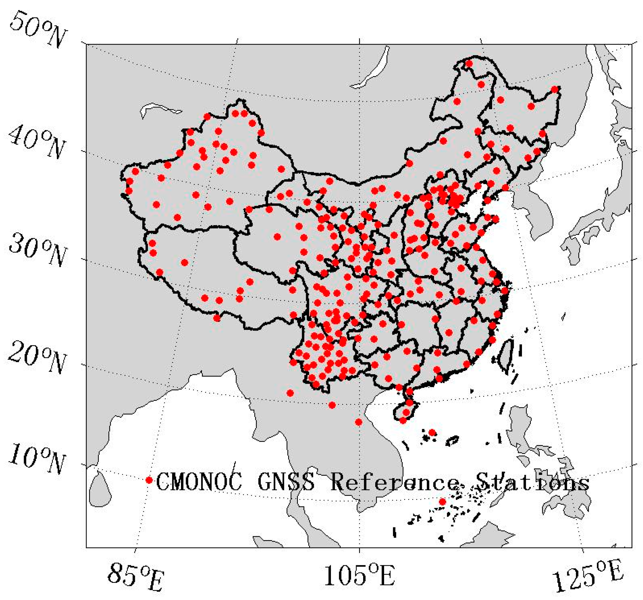
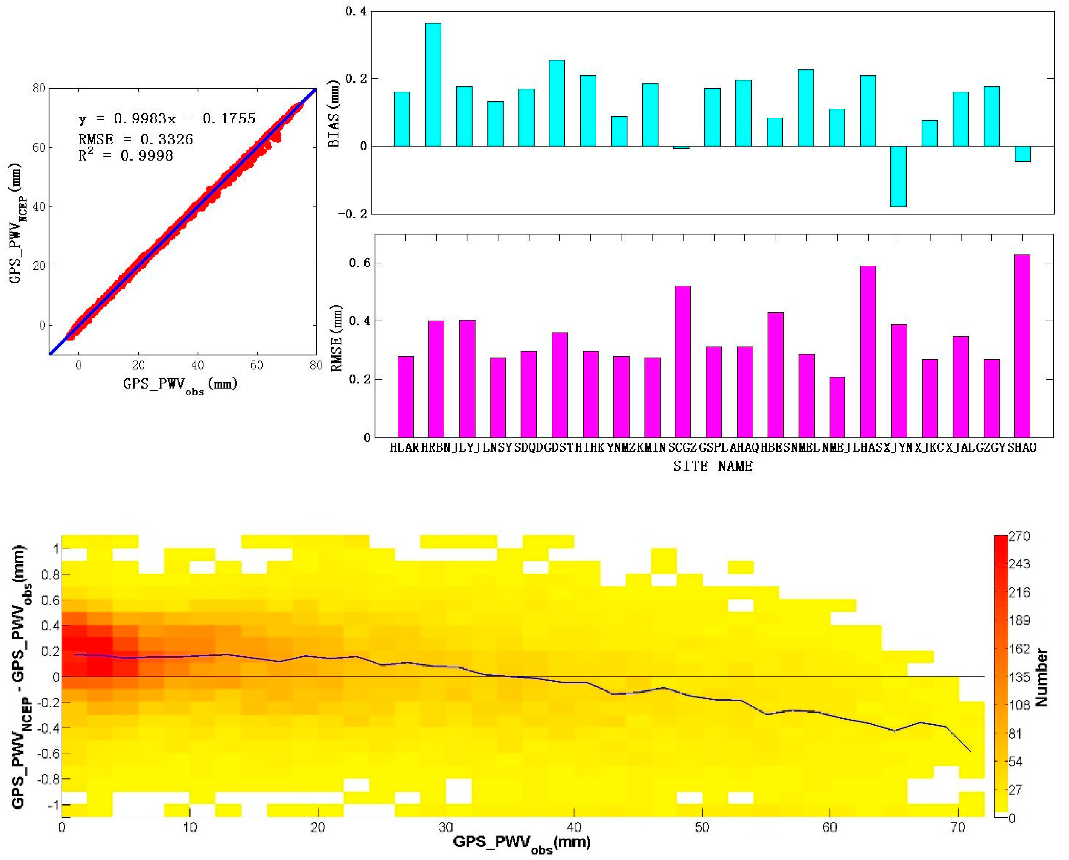
- At the 22 CMONOC GNSS stations, we first employed GAMIT software to process GPS data under ITRF2008. The cut-off elevation angle was 10°, and ZTD was estimated with the GMF mapping function at each station. Because of the long distances between our selected stations, absolute ZTD and atmospheric delay horizontal gradient values, at intervals of one hour and two hours respectively, could be estimated directly without introducing any other GPS sites into this network. Then, we calculated GPS PWV, as described in Section 2.1. Real surface pressure measurements of Ps and Tm were computed from real near-ground air temperature observations Ts. We denoted the PWV results as GPS_PWVobs.
- (2)
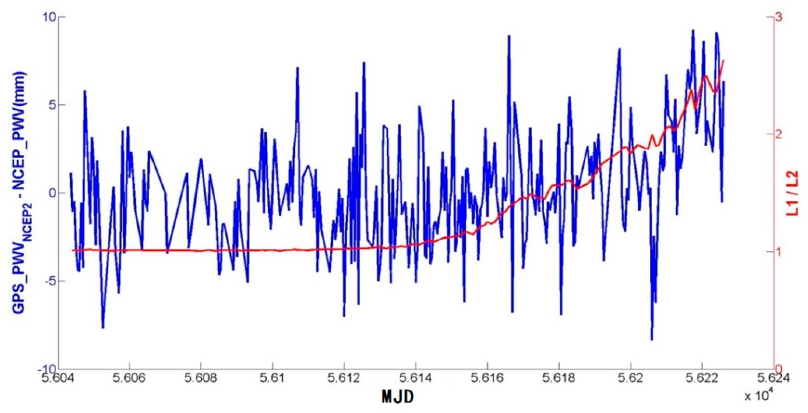
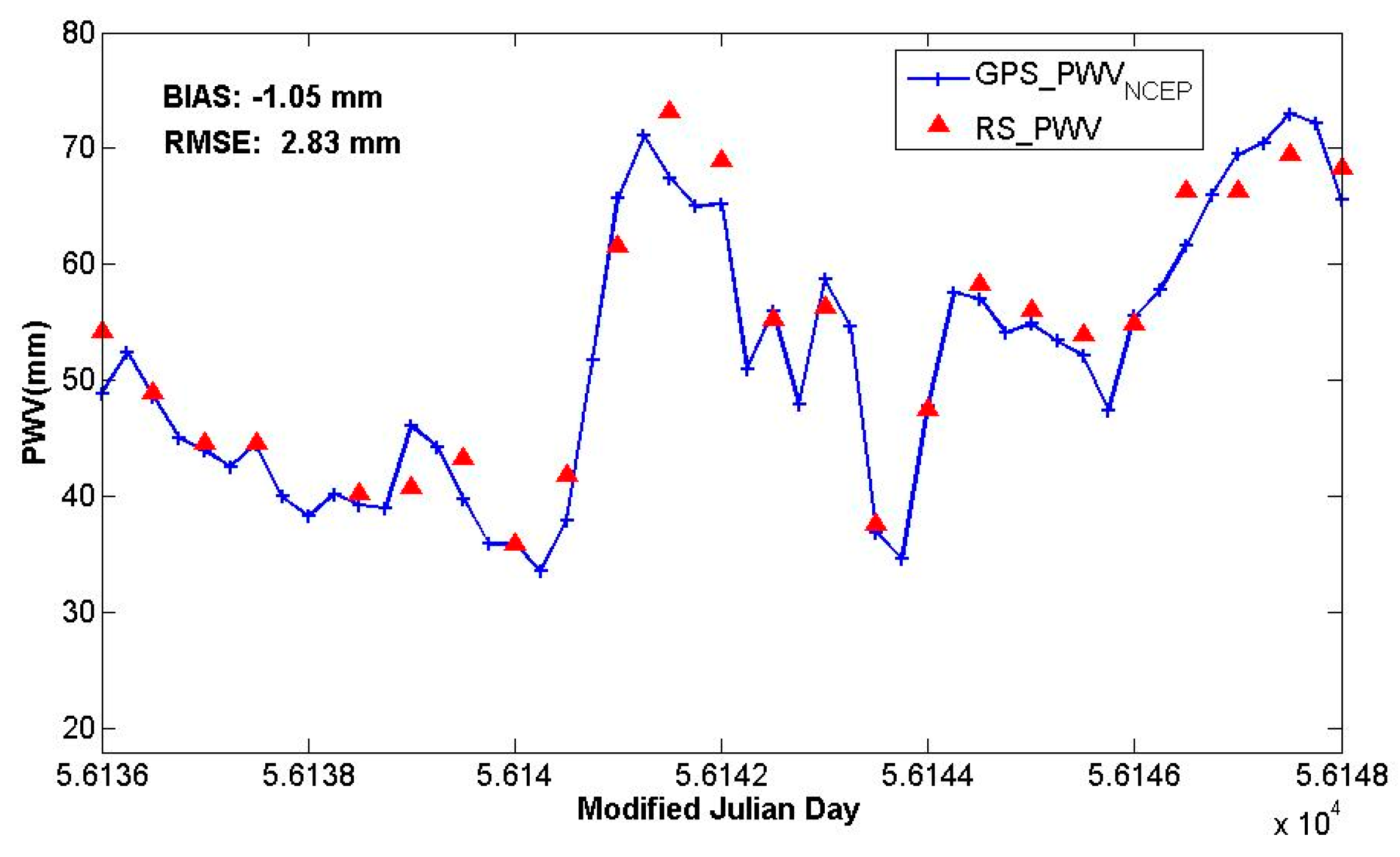
- This scheme is similar to method (1), expect that Ps and Ts were generated from the interpolation of the NCEP FNL dataset, as proposed in Section 2.2. These GPS PWV results are referred to as GPS_PWVNCEP.
- (3)
- PWV can be integrated from the vertical profile of several meteorological parameters using the following formula:
- (4)
- PWV can also be integrated from NCEP FNL data using the same integral formula as Equation (19) and is referred to as NCEP_PWV.
5. Conclusions and Outlook
Acknowledgments
Author Contributions
Conflicts of Interest
References
- Kudo, T.; Kawamura, R.; Hirata, H.; Ichiyanagi, K.; Tanoue, M.; Yoshimura, K. Large-scale vapor transport of remotely evaporated seawater by a rossby wave response to typhoon forcing during the Baiu/Meiyu season as revealed by the JRA-55 reanalysis. J. Geophys. Res. Atmos. 2014, 119, 8825–8838. [Google Scholar] [CrossRef]
- Lee, J.; Park, J.-U.; Cho, J.; Baek, J.; Kim, H.W. A characteristic analysis of fog using GPS-derived integrated water vapour. Meteorol. Appl. 2010, 17, 463–473. [Google Scholar] [CrossRef]
- Cadeddu, M.P.; Liljegren, J.C.; Turner, D.D. The atmospheric radiation measurement (ARM) program network of microwave radiometers: Instrumentation, data, and retrievals. Atmos. Meas. Tech. 2013, 6, 2359–2372. [Google Scholar] [CrossRef]
- Bevis, M.; Businger, S.; Herring, T.A.; Rocken, C.; Anthes, R.A.; Ware, R.H. GPS meteorology: Remote sensing of atmospheric water vapor using the global positioning system. J. Geophys. Res. Atmos. 1992, 97, 15787–15801. [Google Scholar] [CrossRef]
- Haase, J.; Ge, M.; Vedel, H.; Calais, E. Accuracy and variability of GPS tropospheric delay measurements of water vapor in the western mediterranean. J. Appl. Meteorol. 2003, 42, 1547–1568. [Google Scholar] [CrossRef]
- Pacione, R.; Vespe, F. Comparative studies for the assessment of the quality of near-real-time GPS-derived atmospheric parameters. J. Atmos. Ocean. Technol. 2008, 25, 701–714. [Google Scholar] [CrossRef]
- Khodayar, S.; Kalthoff, N.; Wickert, J.; Kottmeier, C.; Dorninger, M. High-resolution representation of the mechanisms responsible for the initiation of isolated thunderstorms over flat and complex terrains: Analysis of csip and cops cases. Meteorol. Atmos. Phys. 2013, 119, 109–124. [Google Scholar] [CrossRef]
- Smith, T.L.; Benjamin, S.G.; Gutman, S.I.; Sahm, S. Short-range forecast impact from assimilation of GPS-IPW observations into the rapid update cycle. Mon. Weather Rev. 2007, 135, 2914–2930. [Google Scholar] [CrossRef]
- Nilsson, T.; Elgered, G. Long-term trends in the atmospheric water vapor content estimated from ground-based GPS data. J. Geophys. Res. Atmos. 2008, 113. [Google Scholar] [CrossRef]
- Vey, S.; Dietrich, R.; Ruelke, A.; Fritsche, M.; Steigenberger, P.; Rothacher, M. Validation of precipitable water vapor within the NCEP/DOE reanalysis using global GPS observations from one decade. J. Clim. 2010, 23, 1675–1695. [Google Scholar] [CrossRef]
- Sun, B.; Wang, H. Water vapor transport paths and accumulation during widespread snowfall events in northeastern China. J. Clim. 2013, 26, 4550–4566. [Google Scholar] [CrossRef]
- Luo, X.; Heck, B.; Awange, J.L. Improving the estimation of zenith dry tropospheric delays using regional surface meteorological data. Adv. Space Res. 2013, 52, 2204–2214. [Google Scholar] [CrossRef]
- Yao, Y.; Zhang, B.; Xu, C.; Yan, F. Improved one/multi-parameter models that consider seasonal and geographic variations for estimating weighted mean temperature in ground-based GPS meteorology. J. Geod. 2014, 88, 273–282. [Google Scholar] [CrossRef]
- Adams, D.K.; Fernandes, R.M.S.; Kursinski, E.R.; Maia, J.M.; Sapucci, L.F.; Machado, L.A.T.; Vitorello, I.; Monico, J.F.G.; Holub, K.L.; Gutman, S.I.; et al. A dense GNSS meteorological network for observing deep convection in the amazon. Atmos. Sci. Lett. 2011, 12, 207–212. [Google Scholar] [CrossRef]
- Shoji, Y. A study of near real-time water vapor analysis using a nationwide dense GPS network of Japan. J. Meteorol. Soc. Jpn. 2009, 87, 1–18. [Google Scholar] [CrossRef]
- Saastamoinen, J. Atmospheric correction for the troposphere and stratosphere in radio ranging of satellites. Use Artif. Satell. Geod. 1972, 15, 274–251. [Google Scholar]
- Jade, S.; Vijayan, M.S.M. GPS-based atmospheric precipitable water vapor estimation using meteorological parameters interpolated from NCEP global reanalysis data. J. Geophys. Res. Atmos. 2008, 113. [Google Scholar] [CrossRef]
- Vey, S.; Dietrich, R.; Fritsche, M.; Ruelke, A.; Steigenberger, P.; Rothacher, M. On the homogeneity and interpretation of precipitable water time series derived from global GPS observations. J. Geophys. Res. Atmos. 2009, 114. [Google Scholar] [CrossRef]
- Karabatic, A.; Weber, R.; Haiden, T. Near real-time estimation of tropospheric water vapour content from ground based GNSS data and its potential contribution to weather now-casting in Austria. Adv. Space Res. 2011, 47, 1691–1703. [Google Scholar] [CrossRef]
- Bosy, J.; Kaplon, J.; Rohm, W.; Sierny, J.; Hadas, T. Near real-time estimation of water vapour in the troposphere using ground GNSS and the meteorological data. Ann. Geophys. 2012, 30, 1379–1391. [Google Scholar] [CrossRef]
- Means, J.D.; Cayan, D. Precipitable water from GPS zenith delays using North American regional reanalysis meteorology. J. Atmos. Ocean. Technol. 2013, 30, 485–495. [Google Scholar] [CrossRef]
- Means, J.D. GPS precipitable water as a diagnostic of the North American monsoon in California and Nevada. J. Clim. 2013, 26, 1432–1444. [Google Scholar] [CrossRef]
- Chen, J.; Zhang, P. On the national projects for surveying and mapping datum in the twelfth five year plan of China. Geomat. Inf. Sci. Wuhan Univ. 2009, 34, 1135–1138. [Google Scholar]
- Wang, H.; Wei, M.; Li, G.; Zhou, S.; Zeng, Q. Analysis of precipitable water vapor from GPS measurements in Chengdu region: Distribution and evolution characteristics in autumn. Adv. Space Res. 2013, 52, 656–667. [Google Scholar]
- Xie, Y.; Wei, F.; Chen, G.; Zhang, T.; Hu, L. Analysis of the 2008 heavy snowfall over south China using GPS PWV measurements from the Tibetan plateau. Ann. Geophys. 2010, 28, 1369–1376. [Google Scholar] [CrossRef] [Green Version]
- Dousa, J. The impact of errors in predicted GPS orbits on zenith troposphere delay estimation. GPS Solut. 2010, 14, 229–239. [Google Scholar] [CrossRef]
- Duan, J.; Bevis, M.; Fang, P.; Bock, Y.; Chiswell, S.; Businger, S.; Rocken, C.; Solheim, F.; van Hove, T.; Ware, R.; et al. GPS meteorology: Direct estimation of the absolute value of precipitable water. J. Appl. Meteorol. 1996, 35, 830–838. [Google Scholar] [CrossRef]
- Bevis, M.; Businger, S.; Chiswell, S.; Herring, T.A.; Anthes, R.A.; Rocken, C.; Ware, R.H. GPS meteorology: Mapping zenith wet delays onto precipitable water. J. Appl. Meteorol. 1994, 33, 379–386. [Google Scholar] [CrossRef]
- Wang, J.H.; Zhang, L.Y.; Dai, A. Global estimates of water-vapor-weighted mean temperature of the atmosphere for GPS applications. J. Geophys. Res. Atmos. 2005, 110. [Google Scholar] [CrossRef]
- Bonafoni, S.; Mazzoni, A.; Cimini, D.; Montopoli, M.; Pierdicca, N.; Basili, P.; Ciotti, P.; Carlesimo, G. Assessment of water vapor retrievals from a GPS receiver network. GPS Solut. 2013, 17, 475–484. [Google Scholar] [CrossRef]
- Deng, Z.; Bender, M.; Zus, F.; Ge, M.; Dick, G.; Ramatschi, M.; Wickert, J.; Lhnert, U.; Schon, S. Validation of tropospheric slant path delays derived from single and dual frequency GPS receivers. Radio Sci. 2011, 46. [Google Scholar] [CrossRef]
- Wang, J.; Zhang, L.; Dai, A.; Van Hove, T.; Van Baelen, J. A near-global, 2-hourly data set of atmospheric precipitable water from ground-based GPS measurements. J. Geophys. Res. Atmos. 2007, 112. [Google Scholar] [CrossRef]
- Sheng, P.; Mao, J.; Li, J.; Ge, Z.; Zhang, A.; Sang, J.; Pan, N.; Zhang, H. Atmospheric Physics; Peking University Press: Beijing, China, 2003. [Google Scholar]
- Zhang, C.; Guo, C.; Chen, J.; Zhang, L.; Wang, B. EGM 2008 and its application analysis in Chinese mainland. Acta Geod. Cartograph. Sin. 2009, 38, 283–289. [Google Scholar]
- Smith, A.; Lott, N.; Vose, R. The integrated surface database recent developments and partnerships. Bull. Am. Meteorol. Soc. 2011, 92, 704–708. [Google Scholar] [CrossRef]
- Boehm, J.; Heinkelmann, R.; Schuh, H. Short note: A global model of pressure and temperature for geodetic applications. J. Geod. 2007, 81, 679–683. [Google Scholar] [CrossRef]
- Hardy, B. Its-90 formulations for vapor pressure, frostpoint temperature, dewpoint temperature, and enhancement factors in the range −100 to +100 c. In Proceedings of the Third International Symposium on the Humidity & Moisture, London, UK, 6–8 April 1998.
- Wang, X.; Dai, Z.; Cao, Y.; Song, L. Weighted mean temperature tm statistical analysis in ground-based GPS in China. Geomat. Inf. Sci. Wuhan Univ. 2011, 36, 412–416. [Google Scholar]
- Liang, H.; Cao, Y.; Wan, X.; Xu, Z.; Wang, H.; Hu, H. Meteorological applications of precipitable water vapor measurements retrieved by the national GNSS network of China. Geod. Geodyn. 2015, 6, 135–142. [Google Scholar] [CrossRef]
- Perez-Ramirez, D.; Whiteman, D.N.; Smirnov, A.; Lyamani, H.; Holben, B.N.; Pinker, R.; Andrade, M.; Alados-Arboledas, L. Evaluation of Aeronet precipitable water vapor versus microwave radiometry, GPS, and radiosondes at ARM sites. J. Geophys. Res. Atmos. 2014, 119, 9596–9613. [Google Scholar] [CrossRef]
- De Galisteo, J.P.O.; Toledano, C.; Cachorro, V.; Torres, B. Improvement in PWV estimation from GPS due to the absolute calibration of antenna phase center variations. GPS Solut. 2010, 14, 389–395. [Google Scholar] [CrossRef]


| Value Domain | Absolute BIAS as Statistics | RMSE as Statistics | ||
|---|---|---|---|---|
| ISD | CMONOC | ISD | CMONOC | |
| ≤1 hPa | 356 | 200 | 318 | 158 |
| 1 ~ 2.8 hPa | 17 | 36 | 55 | 76 |
| 2.8 ~ 5 hPa | 2 | 3 | 2 | 5 |
| ≥5 hPa | 1 | 1 | 1 | 1 |
| Value Domain | Absolute BIAS as Statistics | RMSE as Statistics | ||
|---|---|---|---|---|
| ISD | CMONOC | ISD | CMONOC | |
| ≤5.0 K | 373 | 232 | 365 | 226 |
| >5.0 K | 3 | 8 | 11 | 14 |
| GNSS Station | lat (°) | lon (°) | Height (m) | RS Station | lat (°) | lon (°) | Height (m) |
|---|---|---|---|---|---|---|---|
| HLAR | 49.27 | 119.74 | 627.89 | 50527 | 49.22 | 119.75 | 611.00 |
| HRBN | 45.70 | 126.62 | 197.44 | 50953 | 45.68 | 126.62 | 143.00 |
| JLYJ | 42.87 | 129.50 | 283.79 | 54292 | 42.88 | 129.47 | 178.00 |
| LNSY | 41.83 | 123.58 | 69.02 | 54342 | 41.82 | 123.55 | 43.00 |
| SDQD | 36.08 | 120.30 | 12.78 | 54857 | 36.07 | 120.33 | 77.00 |
| GDST | 23.42 | 116.60 | 30.93 | 59316 | 23.35 | 116.68 | 3.00 |
| HIHK | 19.99 | 110.25 | 54.55 | 59758 | 20.03 | 110.35 | 24.00 |
| YNMZ | 23.36 | 103.40 | 1274.50 | 56985 | 23.38 | 103.38 | 1302.00 |
| KMIN | 25.03 | 102.80 | 1985.37 | 56778 | 25.02 | 102.68 | 1892.00 |
| SCGZ | 31.61 | 100.02 | 3352.28 | 56146 | 31.63 | 99.98 | 3394.00 |
| GSPL | 35.55 | 106.59 | 1408.69 | 53915 | 35.55 | 106.67 | 1348.00 |
| AHAQ | 30.62 | 116.99 | 57.75 | 58424 | 30.52 | 117.03 | 20.00 |
| HBES | 30.28 | 109.49 | 472.38 | 57447 | 30.27 | 109.48 | 458.00 |
| NMEL | 43.63 | 111.94 | 945.34 | 53068 | 43.65 | 112.00 | 966.00 |
| NMEJ | 41.96 | 101.06 | 888.42 | 52267 | 41.98 | 101.07 | 941.00 |
| LHAS | 29.66 | 91.10 | 3623.82 | 55591 | 29.70 | 91.13 | 3650.00 |
| XZNQ | 31.49 | 92.11 | 4572.55 | 55299 | 31.48 | 92.05 | 4508.00 |
| XJYN | 43.97 | 81.53 | 732.88 | 51431 | 43.95 | 81.33 | 664.00 |
| XJKC | 41.73 | 82.98 | 1028.08 | 51644 | 41.72 | 82.95 | 1100.00 |
| XJAL | 47.86 | 88.13 | 874.10 | 51076 | 47.73 | 88.08 | 737.00 |
| GZGY | 26.47 | 106.67 | 1093.13 | 57816 | 26.48 | 106.65 | 1222.00 |
| SHAO | 31.10 | 121.20 | 22.02 | 58362 | 31.40 | 121.47 | 4.00 |
| RS Station Number | RMSE (K) | |
|---|---|---|
| Tm_OW–Tm_RS | Tm_IW–Tm_RS | |
| 50527 | 3.70 | 3.64 |
| 50953 | 4.74 | 4.61 |
| 54292 | 4.20 | 4.33 |
| 54342 | 3.63 | 3.69 |
| 54857 | 3.75 | 3.51 |
| 59316 | 2.25 | 2.10 |
| 59758 | 2.10 | 2.29 |
| 56985 | 2.74 | 3.07 |
| 56778 | 3.10 | 2.94 |
| 56146 | 2.58 | 2.28 |
| 53915 | 3.77 | 3.39 |
| 58424 | 3.33 | 3.24 |
| 57447 | 3.37 | 2.96 |
| 53068 | 4.86 | 4.27 |
| 52267 | 4.83 | 4.08 |
| 55591 | 3.41 | 2.58 |
| 55299 | 4.13 | 4.27 |
| 51431 | 4.01 | 3.25 |
| 51644 | 3.77 | 2.78 |
| 51076 | 3.89 | 3.68 |
| 57816 | 2.15 | 1.99 |
| 58362 | 3.48 | 3.66 |
| Site Name | RMSE (K) |
|---|---|
| XZRT (Tibet) | 3.29 |
| XZGE (Tibet) | 1.44 |
| XZBG (Tibet) | 1.76 |
| XZGZ (Tibet) | 1.98 |
| WUSH (Xingjiang) | 1.95 |
| XJKE (Xingjiang) | 1.39 |
| XJDS (Xingjiang) | 2.32 |
| NMWL (Inner Mongolia) | 2.63 |
| QHWQ (Qinghai) | 2.67 |
| SCPZ (Sichuan) | 5.69 |
| BIAS(mm) | RMSE(mm) | Correlation | |
|---|---|---|---|
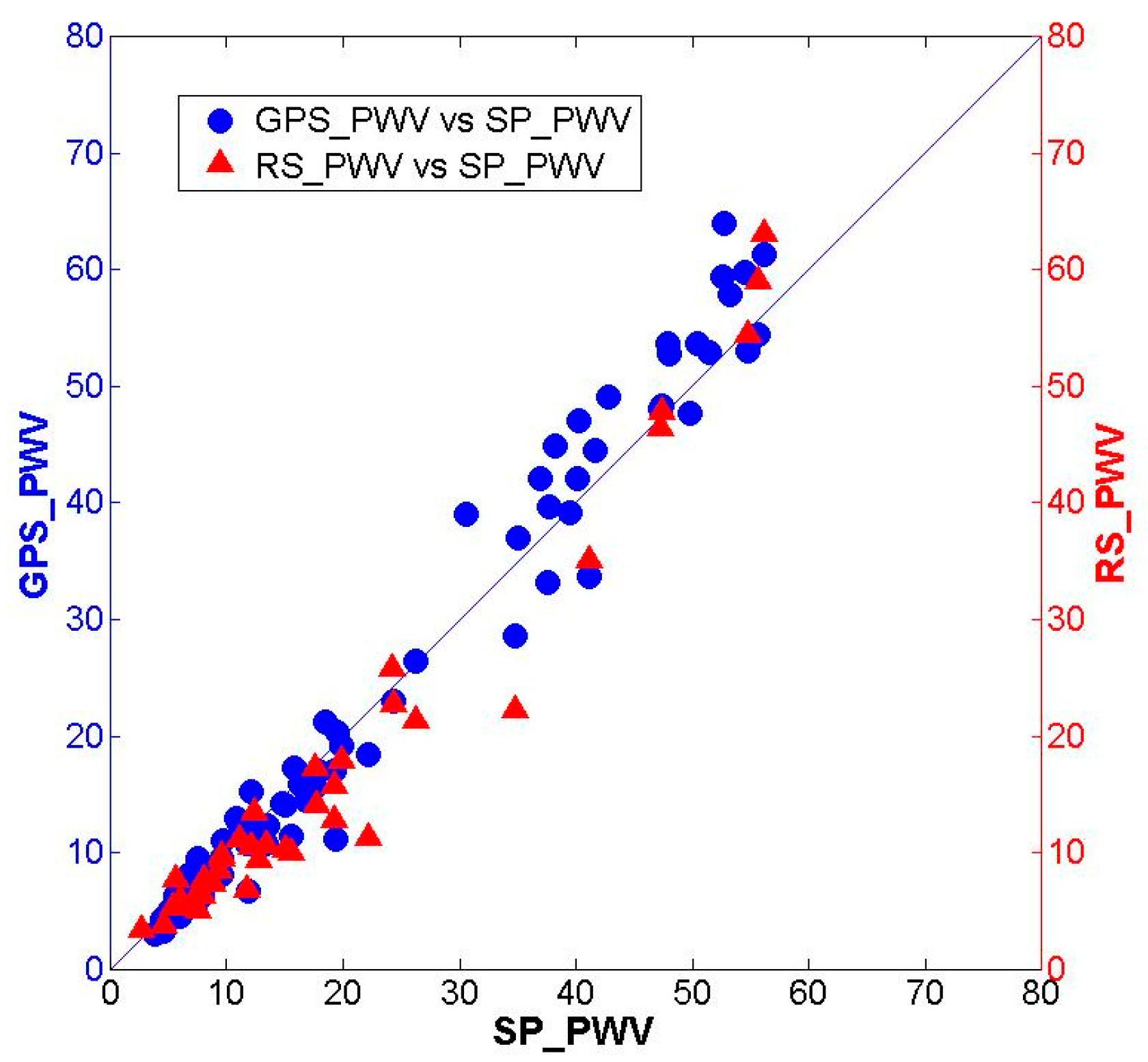
| GPS_PWVNCEP vs. SP_PWV | 0.3464 | 3.3439 | 0.9870 |
| RS_PWV vs. SP_PWV | −1.7908 | 3.8969 | 0.9763 |
© 2016 by the authors; licensee MDPI, Basel, Switzerland. This article is an open access article distributed under the terms and conditions of the Creative Commons Attribution (CC-BY) license (http://creativecommons.org/licenses/by/4.0/).
Share and Cite
Jiang, P.; Ye, S.; Chen, D.; Liu, Y.; Xia, P. Retrieving Precipitable Water Vapor Data Using GPS Zenith Delays and Global Reanalysis Data in China. Remote Sens. 2016, 8, 389. https://doi.org/10.3390/rs8050389
Jiang P, Ye S, Chen D, Liu Y, Xia P. Retrieving Precipitable Water Vapor Data Using GPS Zenith Delays and Global Reanalysis Data in China. Remote Sensing. 2016; 8(5):389. https://doi.org/10.3390/rs8050389
Chicago/Turabian StyleJiang, Peng, Shirong Ye, Dezhong Chen, Yanyan Liu, and Pengfei Xia. 2016. "Retrieving Precipitable Water Vapor Data Using GPS Zenith Delays and Global Reanalysis Data in China" Remote Sensing 8, no. 5: 389. https://doi.org/10.3390/rs8050389