Physical Layer Definition for a Long-Haul HF Antarctica to Spain Radio Link

Abstract

La Salle and the Observatori de l’Ebre (OE) have been involved in a remote sensing project in Antarctica for the last 11 years. The OE has been monitoring the geomagnetic activity for more than twenty years and also the ionospheric activity of the last ten years in the Spanish Antarctic Station Juan Carlos I (ASJI) (62.7${}^{°}$S, 299.6${}^{°}$E). La Salle is finishing the design and testing of a low-power communication system between the ASJI and Cambrils (41.0${}^{°}$N, 1.0${}^{°}$E) with a double goal: (i) the transmission of data from the sensors located at the ASJI and (ii) the performance of an oblique ionospheric sounding of a 12,760 km HF link. Previously, La Salle has already performed sounding and modulation tests to describe the channel performance in terms of availability, Signal-to-Noise Ratio (SNR), Doppler spread and delay spread. This paper closes the design of the physical layer, by means of the channel error study and the synchronization performance, and concludes with a new physical layer proposal for the Oblique Ionosphere Sounder. Narrowband and wideband frames have been defined to be used when the oblique sounder performs as an ionospheric sensor. Finally, two transmission modes have been defined for the modem performance: the High Robustness Mode (HRM) for low SNR hours and the High Throughput Mode (HTM) for the high SNR hours.

1. Introduction

Antarctica is a remote and isolated continent of great interest for the scientific community. Many remote sensors are scattered across the continent to conduct experiments related to different disciplines such as biology, geology and physics, performing experiments that cannot be reproduced anywhere else on Earth. These sensors usually store the data during the winter until they can be downloaded the following summer or send the data periodically via a satellite link. However, in polar zones, the transmission between the sensor and the geostationary satellite is poor, thus, in this context, HF transmission is a good alternative. La Salle, together with the Observatori de l’Ebre (OE), both part of the Universitat Ramon Llull (URL), have been working in a joint research project in Livingston Island (62.7${}^{°}$S, 299.6${}^{°}$E), in the South Shetland archipelago for remote sensing and skywave digital communications modem design to be received in Cambrils, Spain (41.0${}^{°}$N, 1.0${}^{°}$E).

Even though the Spanish Antarctic Station Juan Carlos I (ASJI) is only manned during the Austral summer, the recollection of scientific measurements is continuous. The information that has to be analyzed in almost real-time is transmitted to the OE in Spain through a satellite link. To date, only a part of the recorded geomagnetic data of just one of our two variometers in operation can be sent to the OE by satellite link and made available using the facilities provided by the INTErnational Real-time MAGnetic observatory NETwork (INTERMAGNET). A link based on LEO satellite networks [1,2] would have the capability to cover the polar zones in an efficient manner, but the aim of the project was to develop a proprietary communications system, not depending on any other commercial service or technical support. Furthermore, one of the goals of the project was to design a radiomodem, which could perform as a communications system or an oblique ionospheric sounder itself. So, a radio High Frequency (HF) transmission modem can be seen as either an alternative to satellite or a complementary backup system in case of satellite link failure, in terms of data communication. The reader is referred to [3] for more information about the origin and the history of the project, as well as the reasons to plan a backup data transmission system.

The best transmission scheme for long-haul HF links with extremely low Signal-to-Noise Ratio (SNR) has to be found in order to overcome severe channel transmission conditions. Several standards [4,5] have been studied to be applied in this case, but none of them have succeeded in making the SNR to work in the 12,760 km ionospheric link. Therefore, a new physical layer has to be defined. First, narrowband and wideband soundings were performed in [6], in order to describe the channel performance. Afterwards, the system was improved in terms of sounding frequency availability and number of soundings per day, and more complete results were evaluated in [7], giving more details on the channel parameters. Also several modulation tests using spread spectrum modulations [8] have been performed, as well as Orthogonal Frequency-Division Multiplexing (OFDM) [9] and single carrier modulations [10].

This paper has two main goals. The first one to describe in detail the final HF modem hardware, improved since [6,11]. The second one is to continue the work of [7], explaining the narrowband and wideband soundings. In this paper, we present the study of the synchronization sequences, we analyze the channel error burst rate and we choose the best modulations and their configuration to define a physical layer proposal. In order to define a physical layer, we have identified and evaluated four different transmission situations: (i) narrowband sounding; (ii) wideband sounding; (iii) daytime data transmission and (iv) nighttime data transmission. The design of the frame for each of the above four situations will be described and evaluated in detail and the type of the signal and modulation to be transmitted will be discussed.

This paper is organized as follows. Section 2 describes all the measurements. The communications hardware of the modem is specified in Section 3. Section 4 presents the channel study, synchronization and modulation tests performed to design the physical layer. Section 5 details the physical layer proposal for the four cases concluded from the previous tests. Finally, Section 6 explains the conclusions of our research group in the moment of closing the design of this project.

2. Observatory Measurements

This section describes the main measurements carried out in the ASJI, both related to the ionospheric sounder and the geomagnetic sensors.

2.1. Ionospheric Parameters

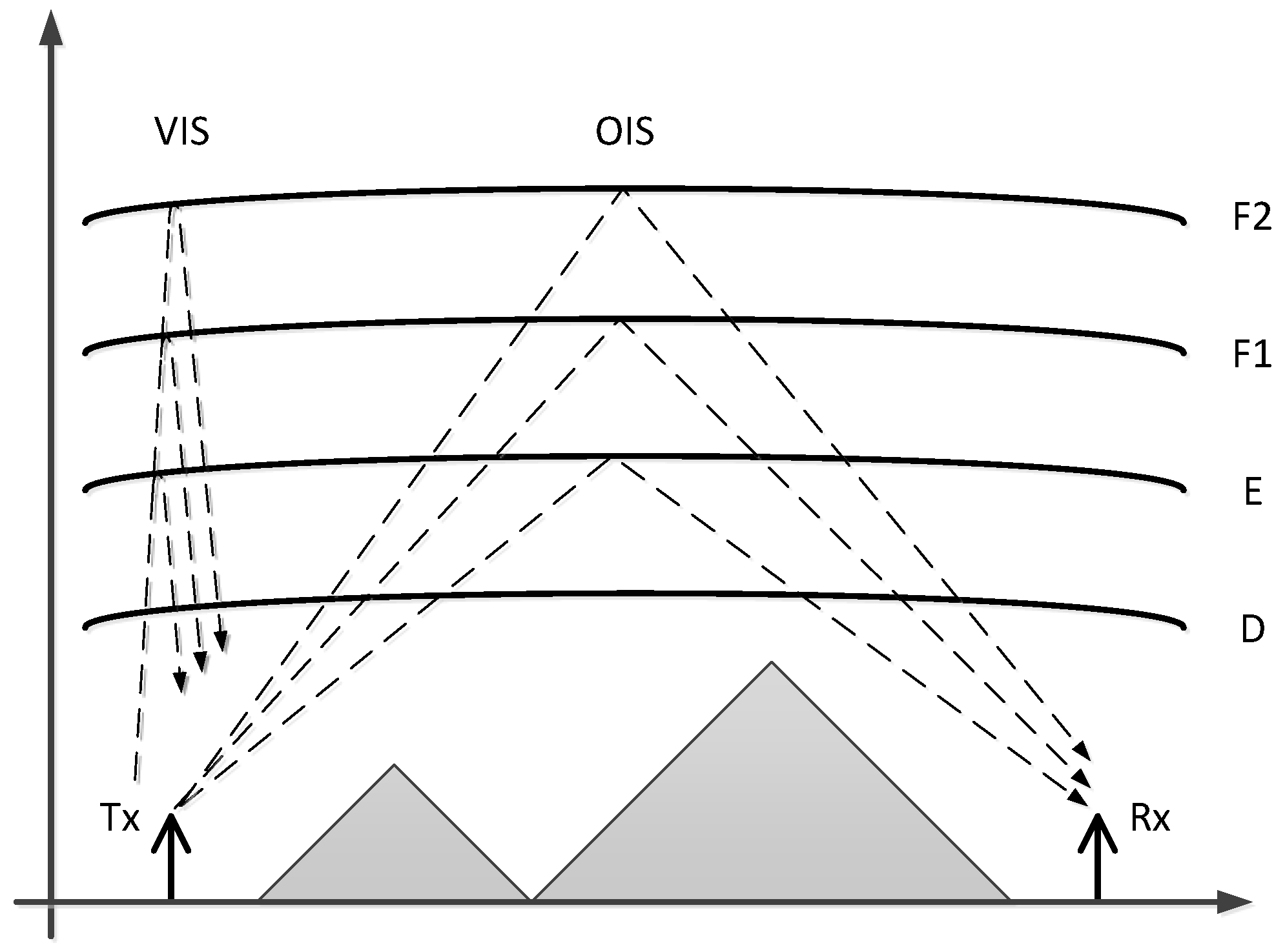
ASJI has two different type of ionospheric sounders operative during the Austral summer: a Vertical Incidence Sounder (VIS) and an Oblique Incidence Sounder (OIS) whose transmitter (Tx) was located in the ASJI and its receiver (Rx) in Spain. Figure 1 [12] shows a simple operation scheme of the vertical incidence and of the oblique incidence.

During the 2004 expedition, the VIS was installed in the ASJI. It records a vertical incidence ionogram every 10 min providing information about the particularities of the ionosphere and helping to model the climatology and the effects of the temporal geomagnetic disturbances. More details on the VIS soundings are given in [13] and details on the instrument, the Advanced Ionospheric Sounder (AIS), developed by the Instituto Nazionale de Geofisica e Vulcanologia (INGV) of Rome, Italy, can be obtained in [14].

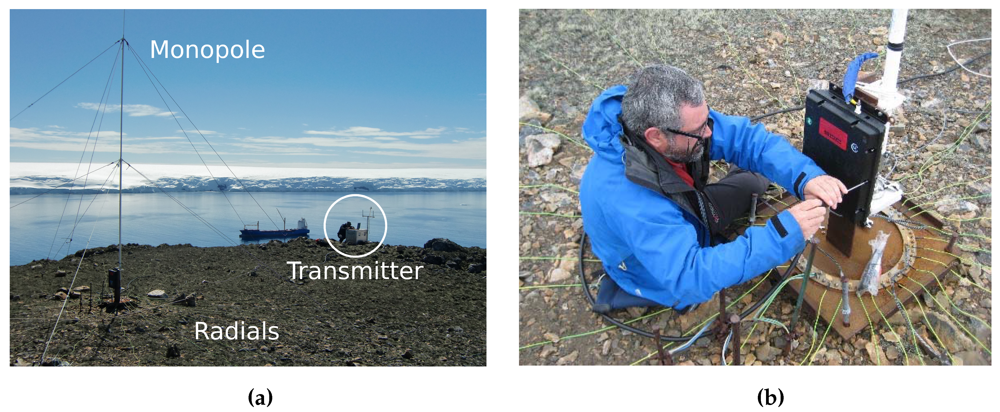
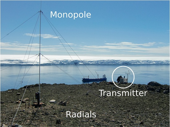
The OIS, developed by La Salle, is used to analyze and characterize the 12,760 km ionospheric channel between Antarctica and Spain [6] during the austral summer, when the ASJI is operative. The key parameters obtained are: (i) link availability; (ii) power delay profile of the channel and (iii) frequency dispersion. These parameters are used to model the HF radio link, with the OIS becoming another useful sensor of the ionosphere. The transmitter antenna is located in the ASJI (see picture in Figure 2a, with the detail of the radials in Figure 2b). More details on the HF data transmission will be described below, in Section 3.

2.2. Geomagnetic Instruments

The measurement of geomagnetic parameters requires considerable experience from both a scientific and technical point of view because the resulting magnitude to be retrieved is a vector. The coordinate systems used in geomagnetism are classified according to its geographic reference.

The main sensors and system of the geomagnetic station are as follows:

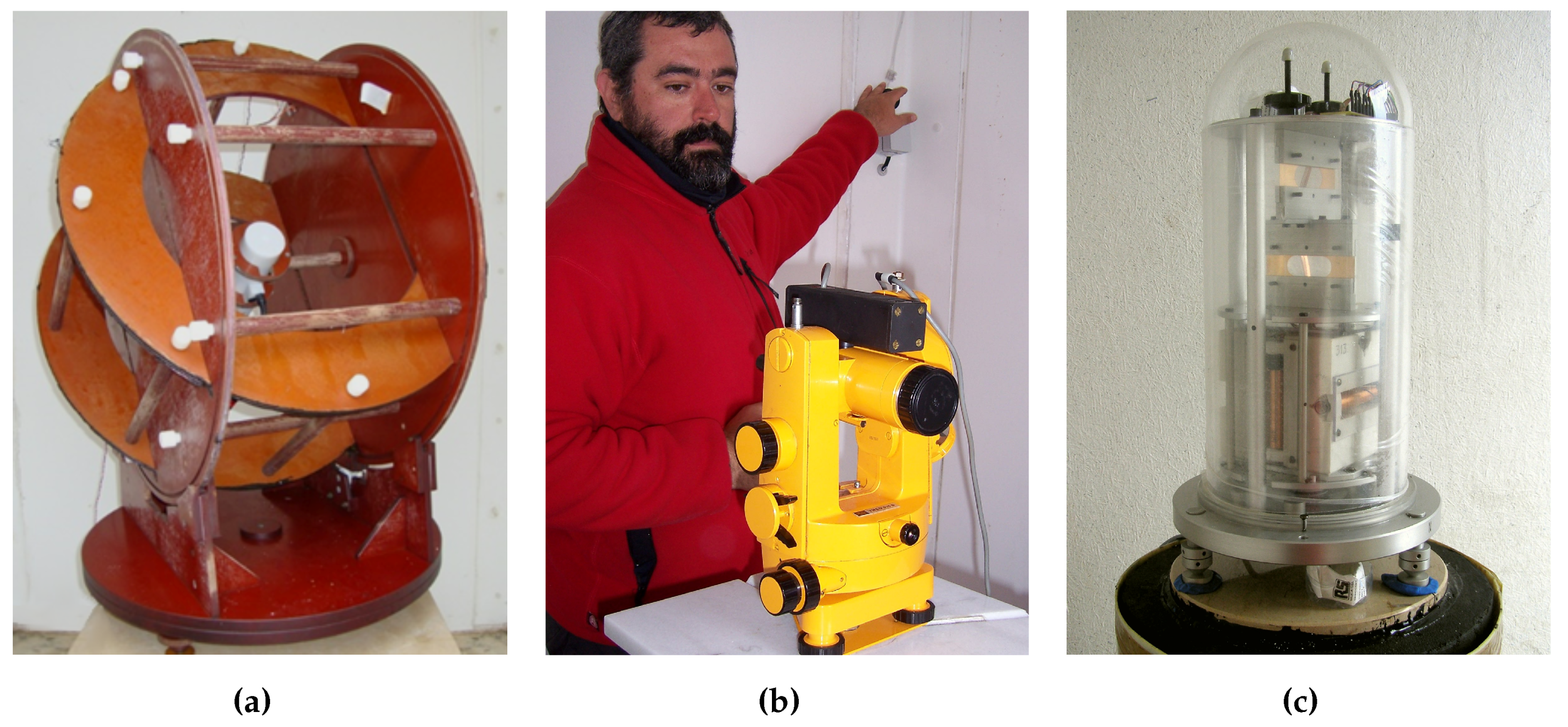
• δD/δI Vector Magnetometer. A δD/δI variometer is mounted in the ASJI to automatically measure (once per minute) the variations of the magnetic field (see Figure 3a). It consists of two pairs of Helmholtz coils positioned perpendicularly and a proton magnetometer located at the center. More details are given in [15]. The proton magnetometer measures the polarization of the coils to acquire the declination and inclination variations and, the value of the total magnetic field intensity is measured when the coils are not polarized [16].
• D/I Fluxgate Theodolite. The huts of the ASJI also contain a declination and inclination (D/I) fluxgate theodolite (see Figure 3b) which is used to manually measure the inclination and declination angles of the magnetic field vector in absolute values. This instrument consists of a fluxgate magnetometer bar mounted on a non-magnetic theodolite telescope, more details in [15]. The uncertainties of this sensor are taken into consideration in [17].
• Three-axis Fluxgate Magnetometer. A three-axis fluxgate magnetometer was added during the 2008 expedition (see Figure 3c). It measures the magnetic field variations automatically sampling an analogue output at both 1 and 0.1 Hz using an Analog-to-Digital Converter (ADC).
• Control System. The electronic system controlling the automatic instruments is also housed indoor in the ASJI. Once the sensors data is processed, the definitive data set is sent to the World Data Centers to become available for the scientific community. The real-time access to the data is provided by a satellite link to the INTERMAGNET. However, a safe skywave link designed by La Salle and the OE is used as a backup. The sensor data can be sent autonomously by the skywave link becoming the channel itself another interesting sensor of the ionosphere.

3. System Description

The main goal of the system is to get the widest possible frequency range as possible and the best time accuracy for the transmission. This involves both the hardware design of the sounders and the data transmission system of the OIS. The initial system was deployed on the first survey (in 2003-04 campaign) [6] but 6 years later (in 2009-10 campaign), an upgraded, faster and more reliable system was placed in Livingston Island to increase the range of the sounding intervals [18]. In such way, a higher bandwidth up to 40 kHz and a sampling frequency of 100 ksps is reached. In addition, concerning the soundings, this system is more flexible in terms of frequency and bandwidth selection.

The following subsections describe the hardware of the transmitter and the receiver.

3.1. Hardware of the Transmitter

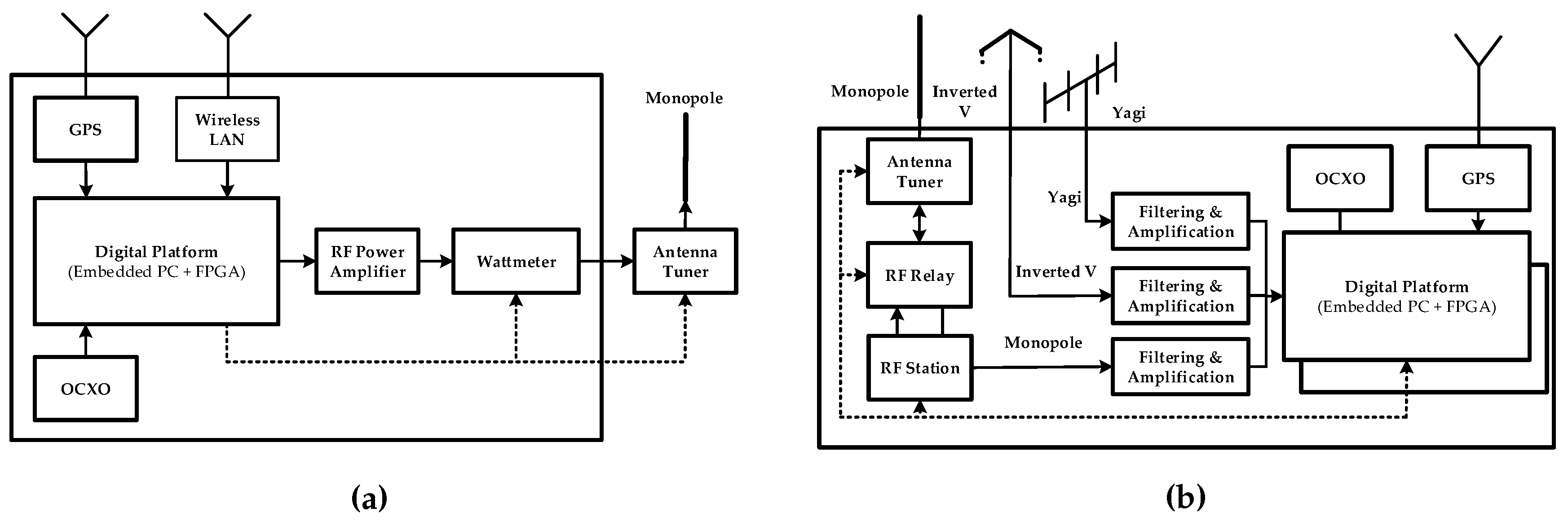
The complete block diagram of the transmitter is shown in Figure 4a. It consists of a digital platform that controls the power amplifier, the Wattmeter and the antenna tuner. The system uses the WiFi for control and configuration purposes, while the Global Positioning System (GPS) and the Oven-Controlled Crystal Oscillator (OCXO) are used for time and frequency synchronization, respectively.

3.1.1. Placement

The transmitter hardware is placed near the antenna at the top of an elevation near the ASJI in a water-sealed box that protects the electronics from weather conditions and provides strong electromagnetic shielding (see Figure 2a). All the inputs and outputs from the box are properly filtered and buccaneer connectors are used for both data and power supply. It has also an air extraction system capable of working under strong winds and snow. The sensors are located near the ASJI so the data has to be sent to the transmitter, which is approximately 150 m away from the sensors. Initially, the communication between the sensors and the transmitter was made via a shielded twisted pair, but it broke several times because of the extreme weather conditions. Then, we decided to transmit the data and the control signals via WiFi from the ASJI, which proved to be a more reliable solution.

3.1.2. Antenna and Antenna Tuner

One of the requirements of a system operating in Antarctica is the low environmental impact, thus, a simple antenna with the maximum of radiation towards the horizon would be desirable. The monopole is one of the most useful antennas suiting this kind of scenario, but an antenna tuner is needed to transmit throughout the whole HF band. Thus, we installed a monopole for signal transmission purposes.

However, when using amateur radio antenna tuners, sometimes the adaptation is not perfect mainly at the lower frequencies of the HF band and one may get high values of Voltage Standing-Wave Ratio (VSWR) with a significant amount of reflected power. Moreover, the monopole is subject to strong winds and extreme weather conditions, so its behavior degrades over time.

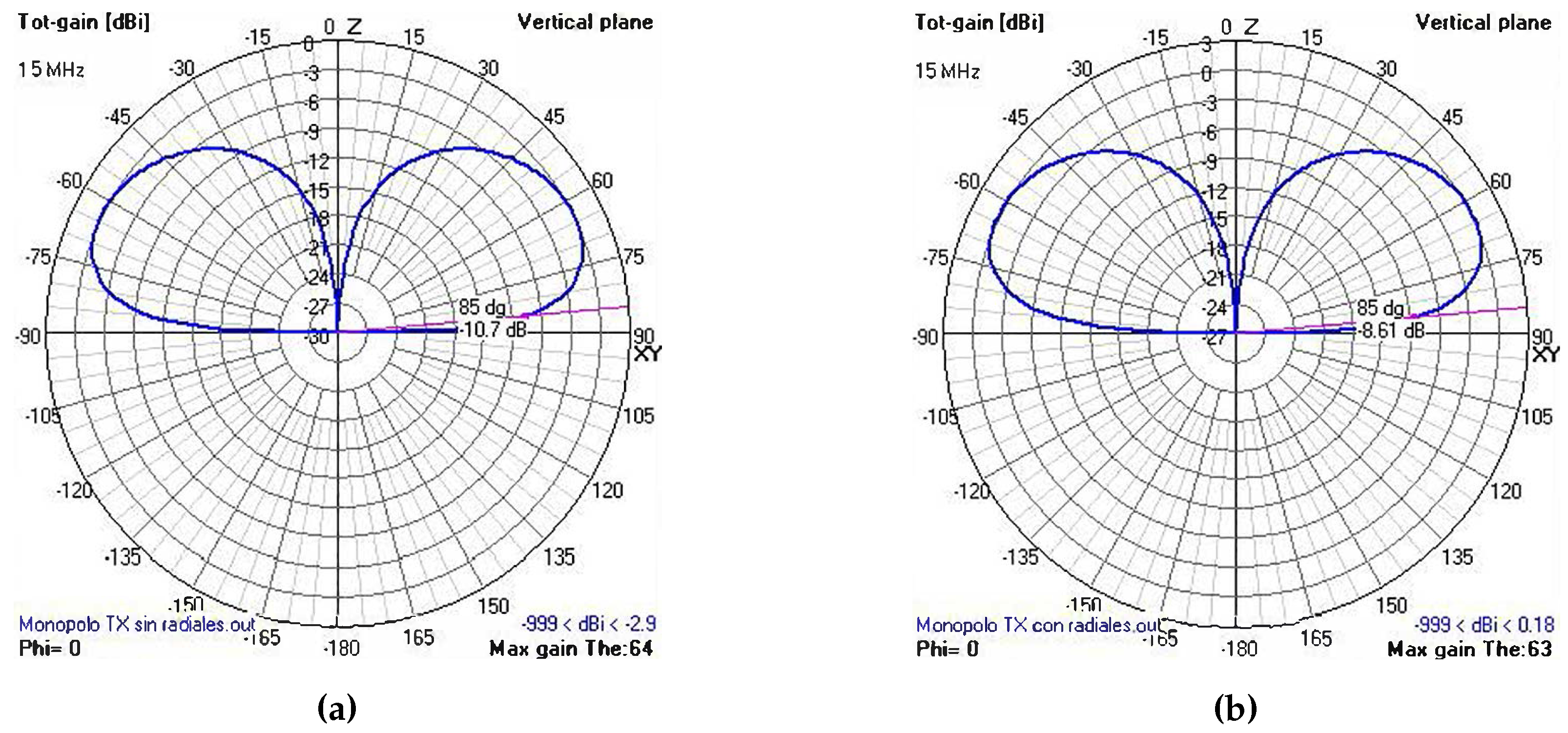
In order to lower the main radiation lobes of the monopole to maximize the gain, we had to improve the conductivity of the ground plane. In Antarctic regions, due to the permafrost found when soil is at or below freezing point, conductivity is far from the ideal value.

Several simulations were conducted to evaluate the change in the gain in elevation angles lower than 11${}^{°}$ from the horizon, depending on the number and the length of the radials of the monopole, and also of the type of terrain. The radial characteristics do not change the adaptation of the antenna tuner, but as the voltage is higher when performing with radials, a more detailed design has to be done to avoid system malfunction.

The simulation software used were 4NEC2 [19] and EZNEC+ [20], both simulation methods for wire antennas, using NEC2 as standard simulation technique, originally developed as NEC by Lawrence Livermore Laboratory [21]. Several simulations were conducted using the classical paradigm of simulation, measuring the change in the gain modifying only one of the simulation parameters (either the number of radials, the length, the section, the type of terrain or the frequency).

Simulations conducted for different types of terrain or frequency did not modify substantially the gain results; the parameters associated to the radial design had a clearer influence in the gain variations. The results, which led us to conclude the best radial characteristics, are shown in Figure 5. They compare the gain at 15 MHz with an elevation of 5${}^{°}$ without and with radials. The results show that the gain increased from $-10.7$ dB without the radials to $-8.6$ dB with the radials. Nearly 2 dB of gain obtained only by choosing 32 radials of 15 m length and 2.5 mm${}^2$ section.

That means an increment of the voltage drop at the antenna terminals, and some additional isolation was needed to avoid the electric arc.

3.1.3. Wattmeter

The antenna tuning procedure became critical for some frequencies and some antenna tuners were damaged during the experimental preliminary tests. Once the adaptation network has been tuned at a certain frequency with a low-power tone, “hold” position was activated to keep the configuration settings. However, when a spread spectrum signal was being transmitted, the device began to re-tune at full power sometimes, ignoring the “hold” signal and, as a result, some relays, inductors and capacitors were burned out.

To overcome the above incidences, a remote controlled VSWR meter was designed. It measured during the whole transmission and warned the control system in case of mismatch to switch off the power amplifier. The block diagram of this VSWR meter is shown in Figure 6. The logarithmic amplifier AD8310, followed by the AD8362 true power detector, detects the forward and reverse power signals from the directional coupler. Concerning the amplifier, it presents a rise time smaller than 15 ns, allowing a quick reaction when a mismatch occurs, and a high dynamic range (up to 95 dB), which is necessary for the detection of a weak reflected signal in the presence of a high power transmitted signal. When the VSWR meter notices the increase in the reverse transmitted power, the control system switches off the amplifier, protecting both the amplifier and the antenna tuner. Since the Wattmeter was put into operation, no other antenna tuner has been damaged, overcoming the aforementioned problems.

Two temperature sensors were installed for further protection: inside (A) and outside (B) the power amplifier box (see Figure 6). When the value from the A or B exceeds a certain threshold, the fans of the power amplifier or the fans of the whole system are activated, respectively. Yet, if the temperature is too high, the transmitter is switched off.

3.1.4. Power Amplifier

The required linearity of the power amplifier is highly dependent on the type of modulation used to transmit the data. Hence, the best choice for sounding the channel is a family of pseudonoise (PN) sequences, due to their optimal auto-correlation and cross-correlation properties. Since the envelope of these sequences is nearly constant, the linearity requirements of the amplifier are not critical. 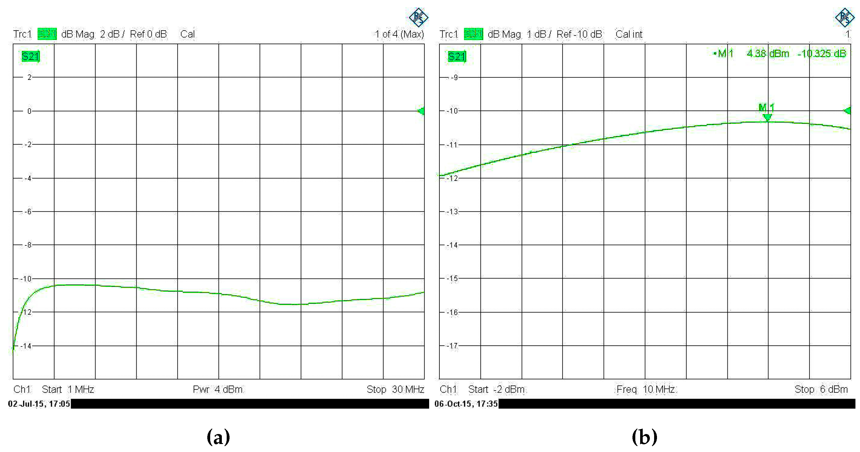However, this type of sequences is not the best option for data transmission and some non-constant envelope modulations have been tested [9,18]. In that case, the linearity of the transmitter is a critical issue, as the non-linear response leads to constellation rotations and noise distortion. A power amplifier of the manufacturer BONN (model BLWA 0103-250) is used, which can reach up to 250 W with an input power lower than 4 dBm. That means a gain of 50 dB, so the amplifier can be fed by the ADC without any additional stage.

The gain fidelity and the linearity were measured using a calibrated network analyzer with a 60 dB attenuator. A variation of less than 1.8 dB from 3 MHz to 30 MHz can be appreciated in Figure 7a, which is an acceptable result for this amplifier. As far as the linearity is concerned, the gain is measured in detail (module of $S_{21}$ [22]) for values of input power between −2 dBm and 6 dBm, as shown in Figure 7b. We can observe variations of the gain from 48 dB to 49.7 dB when the input power varies from −2 dBm to 4.4 dBm. Hence, even if an Input Back-Off (IBO) is applied to keep the average power below the compression point, the gain will not be constant if the signal presents a non-constant envelope. So, in our case, it is worth clipping the signal to keep the average power as constant as possible instead of applying an IBO. This has also been verified by some results showing that the Bit-Error Rate (BER) with strong clipping is the best option for OFDM modulations [9].

3.1.5. Control System

An embedded PC carries out the tasks of controlling and configuring the system with a DSP (Digital Signal Processing) unit inside. The XTremeDSP-IV by Nallatech includes three Xilinx FPGAs (Field-Programmable Gate Array): (i) the Spartan-II connects the interface with the Peripheral Component Interconnect (PCI) bus; (ii) the Virtex-II is in charge of the clock and, finally; (iii) the Virtex-4 conducts the software radio processing with two 14-bit ADCs, two 14-bit DACs (Digital-to-Analog Converter) and the arithmetic and peripheral drivers.

In order to make our measurement system accurate enough, a 100 MHz OCXO with a frequency precision of 30 ppm was installed. This improves the frequency synchronization for OFDM modulations and makes possible the measurement of the Doppler shift. The GPS unit enables the time synchronization using the PPS (Pulse Per Second) signal with an accuracy of 1 μs, so the absolute propagation time from Antarctica to Spain can be measured [11].

3.2. Hardware of the Receiver

The receiver hardware is located in Cambrils, a village located 100 km southwest of Barcelona, in a quiet electromagnetic environment. The block diagram of the receiver is shown in Figure 4b.

The system is able to receive simultaneously from three different antennas. The monopole and the inverted V are both HF antennas with vertical and horizontal polarization, respectively. The third antenna is a Yagi tuned to 14 MHz. This allows performing polarization diversity tests in the whole HF band.

As the monopole is not a wideband antenna, an antenna tuner is needed, even in reception. For the tuning process, a low-power signal (around 10 W) is injected to the antenna during an interval larger than 10 s. This is the reason why a 30 W amplifier is connected to the DAC which generates the tone at the required frequency. The RF (Radio Frequency) relay switches either the adaptation tone (Tx) or the received signal (Rx). The signals from the three antennas are properly filtered, to avoid aliasing and non-desired signals, and amplified to improve the dynamic range of the system.

4. Physical Layer Tests Analysis

In this section, the details of the concluding analysis for the physical layer definition are explained. A short review of the previous sounding and modulations work done over the same channel for previous campaigns will be summarized in the first section. Afterwards, the channel symbol error performance is analyzed, as well as the PN sequence comparison for the best synchronization performance and, finally, all the modulation tests, with both spread spectrum techniques [8] and multi-carrier modulations [18]. The tests presented in this paper were performed over the long-haul channel during several Antarctic campaigns.

Table 1. Detail of the last 5 Antarctic campaigns studied.

Campaign	Starting Date	Ending Date
2009/2010	1 January 2010	2 February 2010
2010/2011	22 January 2011	26 February 2011
2011/2012	30 December 2011	24 February 2012
2012/2013	6 January 2013	22 February 2013
2013/2014	25 January 2014	18 February 2014

provides the time intervals when the tests were carried out in detail.

4.1. Previous Work

Before detailing the novelty of the work in this paper, we detail part of the previous studies performed over the 12,760 km long-haul ionospheric channel.

Soundings of the channel were conducted since 2004 campaign, and their first results were interpreted in [6], with a new digital platform consisting on an FPGA, an Application Specific Integrated Circuit (ASIC) and a high speed D/A converter; it showed results about both narrowband and wideband soundings. 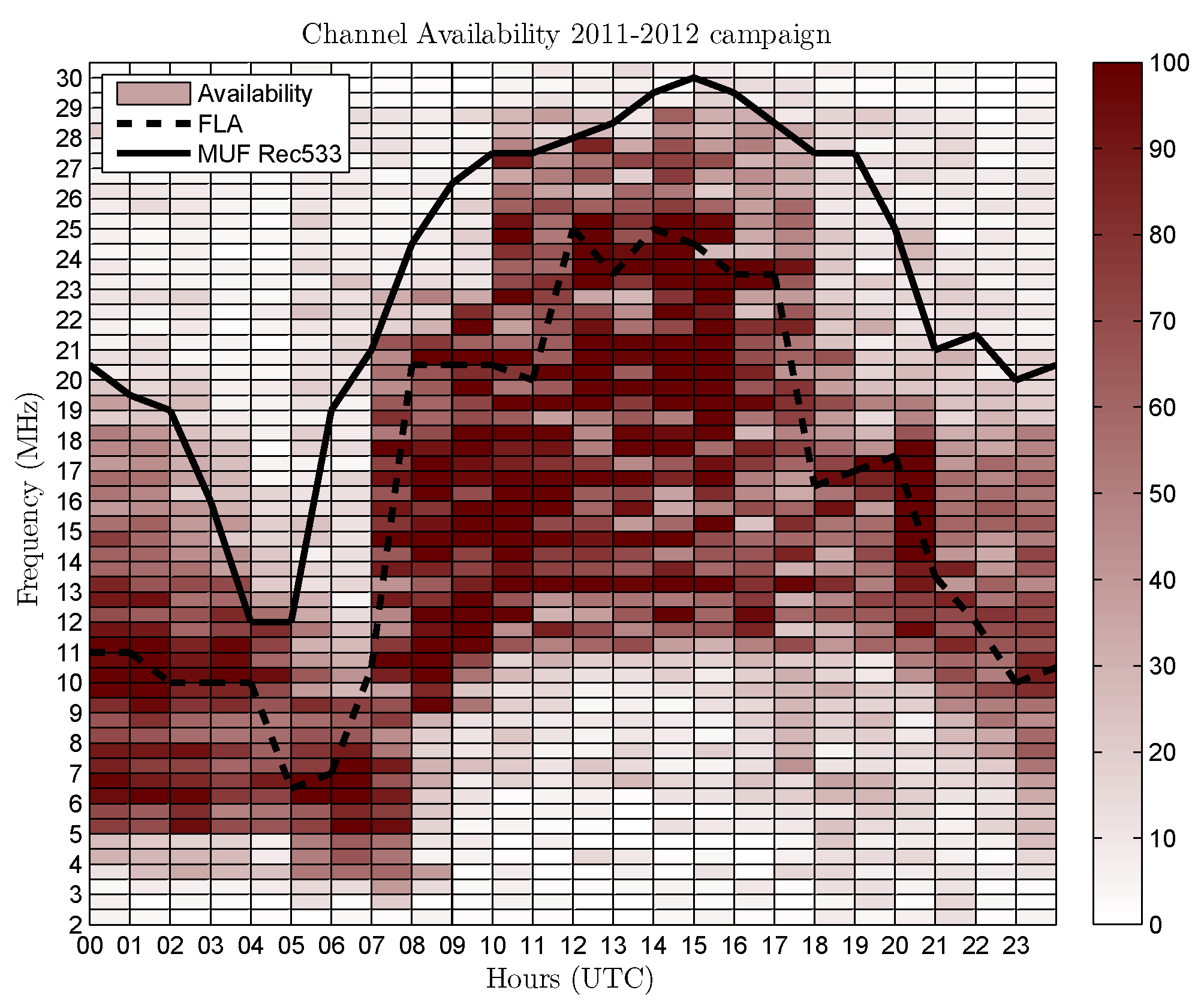Just after that, we improved the sounding measurement in [11] with a new hardware platform (already described in Section 3) and obtained encouraging results in terms of Frequency of Largest Availability (FLA) and availability for all time of the day and frequency sweep. In this moment of the project, the sounding was already obtaining the required data in detail to define the best transmission frequency table once analyzed the FLA for each campaign [23] (see Figure 8 [24]).

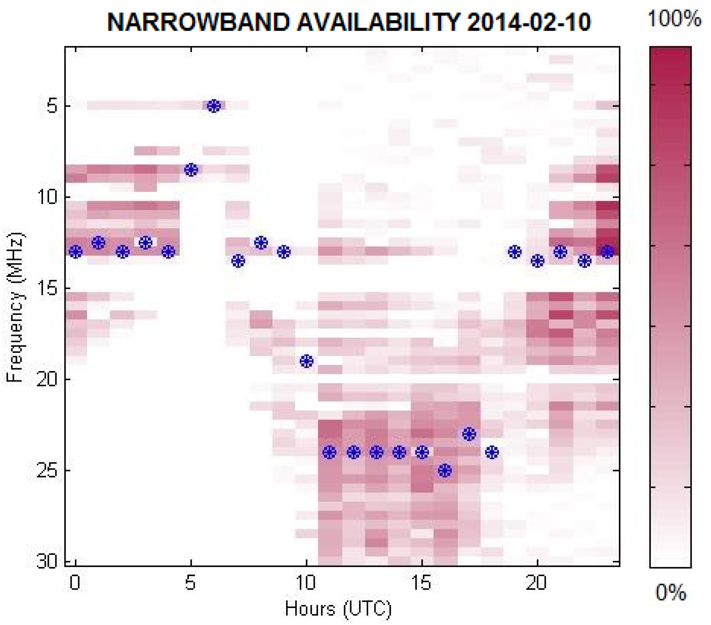
This led the system to settle a table of transmitting frequencies to test the performance of several modulation techniques. See

Table 2. Table of the FLA corresponding to 1 February 2014 measured using the average of the previous 10 days of propagation. Hence, the transmission frequencies are continuously being adapted to the channel performance.

Hour	Frequency	Hour	Frequency	Hour	Frequency
(UTC)	(MHz)	(UTC)	(MHz)	(UTC)	(MHz)
00	13	08	12.5	16	25
01	12.5	09	13	17	23
02	13	10	19	18	24
03	12.5	11	24	19	13
04	13	12	24	20	13.5
05	8.5	13	24	21	13
06	5	14	24	22	13.5
07	13.5	15	24	23	13

for an example of the transmission frequency proposals during the 2014 campaign; they were decided after the availability study averaging the results for several days. Figure 9 compares the selected transmission frequencies to the availability measured a posteriori on a certain day, showing that the best FLA using the 10-day averaging may not always be the best choice at some frequencies for determined day. The transmission frequencies vary depending on the campaign, and even for weeks or days, and have to be redefined while the tests are being conducted in order to adjust their value to the maximum propagation frequency.

As it can be observed in Figure 8 and Figure 9, two propagation zones can be defined, separated by the sunrise and the sunset, which present variable propagation performance [7]. From 00 UTC to 07 UTC, propagation is good at low frequencies, and from 18 UTC to 23 UTC. From 08 UTC to 17 UTC, during daylight hours, the propagation is good at high frequencies. The sunrise (around 07 UTC) and the sunset (around 17 UTC) present unstable performance in terms of propagation, as they are classified as change points from daytime to nighttime. More information about this classification can be found in [6,7,11].

The wideband sounding has also been analyzed in order to determine the maximum delay spread and Doppler spread [6,7,11]. These two channel measures give light to the most suitable modulation for each time of the day and its parameter selection. During all the campaigns, maximum delay spreads observed measure 3.5 ms, this value forces us a minimum symbol time to minimize Intersymbol Interference (ISI). The maximum Doppler spread observed is around 2.5 Hz, thus the coherence time of the channel is around 150 ms, because we defined the coherence time as $T_c=\frac{0.423}{f_D}$ [25]. The reader is referred to [7] for more details about the wideband sounding analysis conclusions and results.

Using the aforementioned frequency transmissions just detailed, and the Doppler and delay spread wideband results, several modulation tests were already conducted in the past. Deumal started with the spread spectrum tests [26], that study let them define the Signaling concept in order to increase the bitrate of the transmission. Also the comparison between Direct-Sequence Spread Spectrum (DS-SS) [27] and OFDM was tested in [9]. The preliminary results obtained by all these tests allowed us to define a modulation testbench including the modulations with best performance and including new modulation schemes to be tested in the channel. The results of this complete analysis will be shown in Section 4.4.

4.2. Channel Error Performance Analysis

The goal in this part of the study is to analyze the symbol error distribution and its impact on the received data for the Signaling modulation scheme.

Direct-Sequence (DS) Signaling is a type of spread spectrum technique that consists in using a whole family of PN sequences as symbols [26] by means of a dictionary, so that each of them is associated to a number of bits. The analysis studies all the received data files, and afterwards, only the synchronized ones are taken into account to evaluate the results.

The PN sequences used in this study are the so called Gold sequences [28] which are suitable codes for this type of modulation due to their trade-off between auto-correlation and cross-correlation properties [29]. Their cross-correlations are low-valued and almost invariant in the whole family. The demodulation method in the channel analysis is a matched filter, so in case of error, the other possible sequences are nearly equiprobable.

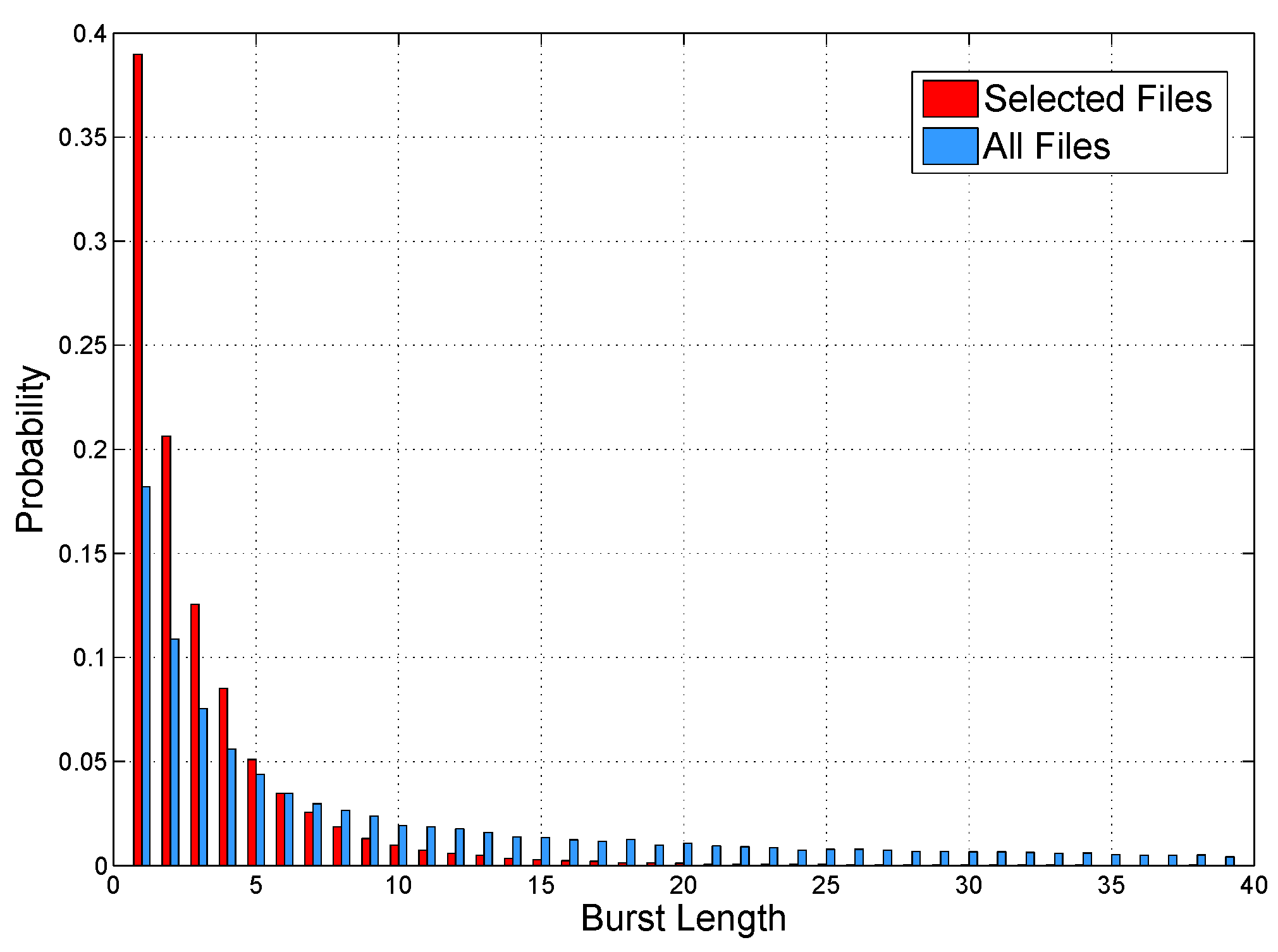
The symbol error burst length is the figure of merit of this analysis, counting the number of consecutive errors that occur in the receiver as the burst length. The probability of appearance of each burst length will be represented in the symbol error burst probability. The first analysis conducted was for all the received files and, afterwards, the results for some selected files were evaluated (see Figure 10).

The results shown in Figure 10 correspond to 120 files of data received on February 2014 (5, 12, 16, 19 and 20). The analysis of all files (without selecting by synchronization) led us to the result of Symbol Error Rate $SER=0.9686$ and $BER=0.4989$, so we can conclude that there were a few data files properly demodulated. The results for the synchronization in the selected files (27 out of 120) show SER and BER values of 0.3157 and 0.1192 respectively. Although these values are high for a regular system, they are acceptable for our modem, designed with retransmission of data, and working in a 12,760 km hostile HF channel.

Figure 10 shows the burst error length probability for both cases and both approach a negative exponential distribution. The most probable value for the burst length is 1, followed by 2 with approximately half the probability, and followed by 3 with a quarter the probability. The probability of having a number of consecutive errors equal or smaller than 3 is over 0.7, which means that almost all the errors appear in a value range from 1 to 3.

The burst error length distribution for the selected files has no significant values for bursts longer than 10; the distribution for all the files has no probability of appearance for bursts longer than 80 symbols.

This led us to the conclusion that most of the errors will appear alone or in a small groups, so that the communications system needs a channel code suitable for short bursts.

4.3. Synchronization Analysis

In this part of the study, we conducted some experiments to determine the best PN sequence to be used for synchronization in this long-haul link. The testbench is based on blocks of 3 PN sequences [30] called training blocks. Two types of PN sequences were tested: m-sequences [28,29] and CAZAC [31]. For each type of sequence, four chip lengths were used: 255, 511, 1023 and 2047. Three different upsample factors (6, 8 and 10) were applied to each of the sequences. The test bandwidths were chosen based on the knowledge obtained from previous tests that used spread spectrum techniques [8,9].

This testbench has two different objectives: (i) identifying the differences in the performance between m-sequences and CAZAC sequences and (ii) obtaining the combination of chip length and bandwidth, which provides the best performance for our scenario.

Maximum peak signal versus the mean signal amplitude of the synchronization triplet correlated with the received one (from now, Max/Mean) is the selected figure of merit in the performed tests. The choice of this figure is based on the statement that in terms of synchronization, it is crucial to find the acquisition point minimizing the false alarm probability. The Max/Mean value fulfills this condition. The Max/Mean value is then normalized dividing it by the length of each sequence. The resulting measure gives a sense of synchronization taking into account the length of each tested sequence. If the measure was not normalized, the longest sequence in terms of Max/Mean would always be the best.

Table 3. Table with the results of the tests: CAZAC sequences vs m-sequences, bandwidth (BW) of 10 kHz, 12 kHz or 16 kHz, and PN sequence length of 255, 511, 1023 and 2047 chips. The bold results show the best Max/Mean rations.

PN Length	BW	Norm Max/Mean (CAZAC)	Norm Max/Mean (M)
(chips)	(Hz)	(10−3)	(10−3)
2047	10 k	0.346	0.363
1023	10 k	0.306	0.285
511	10 k	0.747	0.677
255	10 k	1.034	0.962
2047	12 k	0.392	0.331
1023	12 k	0.593	0.457
511	12 k	0.830	0.678
255	12 k	1.150	0.995
2047	16 k	0.386	0.396
1023	16 k	0.559	0.574
511	16 k	0.831	0.842
255	16 k	1.200	1.244

displays the tests of the synchronization analysis from which we can reach the conclusion that the normalized Max/Mean is a PN sequence with length of 255 chips. Moreover, when comparing the bandwidths, the best situation is presented by the wider one, as it performs better against channel selective fading. Another conclusion extracted from the table is that the results show no evidence of significant differences between CAZAC and m-sequences, because high noise and lossy environment dissipates the difference in terms of auto-correlation between both types of sequence.

According to our results we conclude that the most suitable synchronization sequence is the 255 chip, 16 kHz, m-sequence. This synchronization block contains three sequences and lasts for 15.3 ms per sequence, becoming 45.9 ms for the entire block.

4.4. Modulation Tests

In this subsection we compare the results of modulation tests to find the most suitable configuration. The modulation tests have been divided into two categories: (i) spread spectrum modulations, used because of their better robustness and (ii) multi-carrier modulations, applied because of their higher throughput. In this scenario, the most robust modulation is the one that maintains low BER despite adverse channel conditions; so, the priority is the quality of the data received, and not the total amount of data transmitted. The modulation with higher throughput is the one that reaches maximum bitrate maintaining a low BER; so the priority in that case is the total amount of data transmitted, maintaining a minimum BER value in the receiver.

4.4.1. Spread Spectrum Modulations

Spread spectrum tests were performed first using DS-SS modulation, in order to analyze the throughput and BER of the system versus the length of the PN sequence, the bandwidth and the Energy per Bit to Noise power spectral density ratio (Eb/No) [9]. The results in terms of BER for the several possible combinations are shown in

Table 4. Summary of the results for the DS-SS receptions. The bold combinations show the best results in this group of tests. These measures were performed during campaign 2012 (for more details see the operative days in Table 1). Spc. Eff. stands for Spectral Efficiency and it refers to the information rate that can be transmitted over a given bandwidth in a specific communications system, and CDF stands for Cumulative Density Function.

PN seq.	BW	T	Bitrate	Spc. Eff.	CDF	CDF	CDF	CDF
Length	(kHz)	(ms)	(bps)	(bps/Hz)	(10%)	(30%)	(50%)	(70%)
31	20	1.5	645.16	0.032	0.2910	0.3330	0.3330	0.3740
31	10	3.1	322.58	0.032	0.2490	0.3330	0.3740	0.3740
31	5	6.2	161.29	0.032	0.2910	0.3330	0.3740	0.3740
31	2	15.5	64.52	0.032	0	0.0830	0.2490	0.3330
31	1	31.0	32.26	0.032	0	0	0.1240	0.2490
31	0.50	62.0	16.13	0.032	0	0	0.1240	0.2490
31	0.25	124.0	8.06	0.032	0	0	0.0830	0.2490
63	20	3.1	317.46	0.016	0.2910	0.3740	0.3740	0.3740
63	10	6.3	158.73	0.016	0.2910	0.3330	0.3740	0.3740
63	5	12.0	79.36	0.016	0	0.1660	0.2910	0.3330
63	2	31.0	31.75	0.016	0	0.0410	0.0830	0.2080
63	1	63.0	15.87	0.016	0	0.0410	0.1240	0.2910
63	0.50	126.0	7.94	0.016	0	0	0.1240	0.2490
63	0.25	252.0	3.97	0.016	0	0.1240	0.2490	0.3330
127	20	6.3	157.48	0.007	0.2910	0.3330	0.3330	0.3740
127	10	12.7	78.74	0.007	0.1660	0.2910	0.3330	0.3740
127	5	25.4	39.37	0.007	0	0.1240	0.2910	0.3330
127	2	63.0	15.75	0.007	0	0.0410	0.1660	0.2910
127	1	127.0	7.87	0.007	0	0.0830	0.2080	0.2910
127	0.50	254.0	3.94	0.007	0	0.1660	0.2490	0.2910
127	0.25	507.0	1.97	0.007	0.1240	0.2490	0.3330	0.3740

, whose best results led us to a suitable symbol length which performed properly for all spread spectrum tests.

These first results encouraged us to try to improve the bitrate available for that robust modulation, using values of symbol length around the best results obtained in the previous tests (see Table 4). This second study was published in [8] and it used the Signaling and Quasi-Quadriphase approximation for spread spectrum [26].

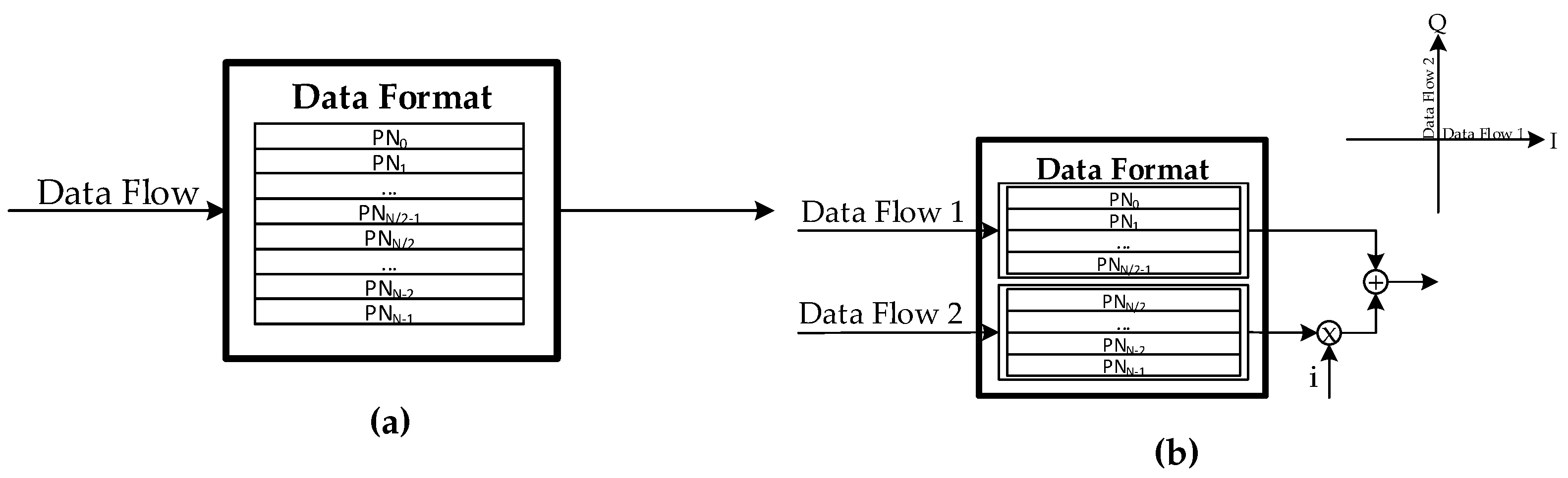
The Signaling, as described in Section 4.2 (see Figure 11a for a graphical description of the modulation structure), and consists in using a whole family of PN sequences as symbols. The information of the transmission will be contained in the proper sequence by means of a codebook. The receiver has the assigned dictionary available. The Quasi-Quadriphase performs the same way using both in-phase and quadrature components (from now, I and Q components) [26], assuming the IQ components orthogonality and the low cross-correlation of the Gold PN sequences associated to the information [28] (see Figure 11b for a graphical detail of the dictionary structure). Therefore, associating information to both I and Q components, we could almost double the throughput of the Signaling option (the throughput is $2n-1$ instead of n bps). The results for these tests are detailed in

Table 5. CDF (Cumulative Density Function) of the BER results for 5% and 10%, sorted from the best (i.e., maximum probability) to the worst results (i.e., minimum probability), for Signaling (S) and Quasi-Quadriphase (QQ) modulations in the bandwidth test. The bold results show the best probabilities of reception.

PN Length	T${}_{\mathit{s}}$	BW	Bitrate	Modulation	BER	BER
	(ms)	(kHz)	(bps)	Scheme	(5%)	(10%)
2047	123	16.6	89	S	0.73	0.81
1023	123	8.3	81	S	0.66	0.79
511	127	4	73	S	0.64	0.78
2047	123	16.6	162.83	QQ	0.56	0.66
255	127	2	65	S	0.53	0.67
511	127	4	125.24	QQ	0.49	0.57
1023	123	8.3	146.62	QQ	0.47	0.58

.

Table 5 shows us bitrates around a hundred of bits per second with reasonable quality assuming we are working in a hostile channel. These results, with high robustness against the channel variations, fading and noise, will lead us to the design of the physical layer for the hours of the day with low availability: during the daytime. In this sense, the best possible combination for the day transmission found is the 2047 PN length, Gold Sequence, with a bandwidth of 16.6 kHz of bandwidth and 89 bps of bitrate [28], performing in Signaling modulation.

4.4.2. Multi-Carrier and Single-Carrier Modulations

Multi-Carrier modulation schemes have been tested to increase the spectral efficiency in comparison to spread spectrum techniques, and so, to increase the bitrate at a reasonable BER.

A first comparison between the DS-SS and OFDM modulation schemes performance was presented in [9] based on real data transmitted from Antarctica to Spain through the HF ionospheric channel. These results encouraged us to do a step forward and propose a single carrier scheme.

A modulation scheme based on a single carrier is proposed in [18] to mitigate the drawbacks of PAPR (Peak-to-Average Power Ratio) [32] and ICI (Inter-Channel Interference) presented on the previous works using OFDM [9]. This modulation scheme is known as Single-Carrier Frequency Domain Equalization (SC-FDE) and has a modulator similar to the OFDM, as detailed in [18].

Several parameters have been modified to study the best configuration for the SC-FDE. These parameters are (i) bandwidths of 400, 800, 1250 and 2500 Hz; (ii) block lengths of 10, 30, 50, 70 and 90 ms and (iii) PSK and Quadrature Phase-Shift Keying (QPSK) constellation. An intensive test of this modulation scheme was done in [10] due to the good results obtained in [18], with real analyzed data transmitted from Antarctica to Spain. The best results in terms of CDF of BER of this experiment are shown in

Table 6. Selected test results for SC-FDE. More results can be found in [10].

Constel.	BW	T${}_{\mathit{b}}$	Bitrate	Spec. Eff.	CDF (BER)
	(Hz)	(ms)	(bps)	(bps/Hz)	(>0.05)
PSK	400	10	296.3	0.74	0.54
PSK	400	30	358.2	0.90	0.56
PSK	400	50	373.8	0.93	0.57
PSK	400	70	381.0	0.95	0.39
PSK	800	10	592.6	0.74	0.40
PSK	800	30	716.4	0.90	0.32
Q-PSK	400	10	592.6	1.48	0.41
Q-PSK	400	30	716.4	1.79	0.42
Q-PSK	400	50	747.7	1.87	0.45
Q-PSK	400	70	761.9	1.90	0.37

.

From this test, we can conclude that the modulation scheme that offers a better performance in terms of a trade-off between BER and bitrate is a PSK of 50 ms and a bandwidth of 400 Hz.

OFDM used in the initial tests [9] can be replaced by a promising technique known as Single-Carrier Frequency-Division Multiple Access (SC-FDMA), because it is less sensitive to ICI and has lower values of PAPR. This technology is based on the OFDM modulator/demodulator, and modified versions of both OFDM and SC-FDMA are compared in [10].

The tests conducted in [10] found a trade-off between the increment of SNR and the Error Vector Magnitude (EVM) to reduce the BER. They took into account several parameter variation for both OFDM and SC-FDMA with IBOs of 1, 4 and 7 dB and 8, 16 and 32 sub-carriers. The results obtained from the analysis with real data are summarized in

Table 7. Best results for OFDM and SC-FDMA with PSK and QPSK constellation that show the CDF (BER) obtained with different configuration parameters. The rows in bold indicate the best BER for each modulation. More results can be found in [10].

Constel.	T${}_{\mathit{b}}$	N${}_{\mathit{c}\mathit{a}\mathit{r}}$	BW	IBO	Bitrate	SC-FDMA	OFDM
	(ms)		(Hz)	(dB)	(bps)	CDF (BER) (>0.05)	CDF (BER) (>0.05)
PSK	10	8	781.3	1	582	0.38	0.38
PSK	20	8	390.6	1	334	0.50	0.72
PSK	20	8	390.6	4	334	0.47	0.34
PSK	40	8	195.3	1	180	0.53	0.50
PSK	40	8	195.3	4	180	0.66	0.50
PSK	40	8	195.3	7	180	0.53	0.53
PSK	40	16	390.6	1	360	0.39	0.53
Q-PSK	20	8	390.6	1	667	0.30	0.34
Q-PSK	20	8	390.6	4	667	0.30	0.39
Q-PSK	40	8	195.3	1	360	0.44	0.47

. From these results, we can observe for OFDM and SC-FDMA that the narrower the waveform, the lower the CDF (BER), because the values of SNR are higher. Moreover, the BER is lower when low values of IBO are applied due to the increment of the mean power, i.e., the SNR increases too. Finally, the sub-carriers of OFDM with a narrower bandwidth produce higher BER because this modulation is sensitive to the ICI.

5. Physical Layer Proposal

In this section, the concluding remarks and the final physical layer proposal will be detailed. All the significant results about previous soundings, channel error study, synchronization and, finally, all modulation tests have been gathered. Following that, a set of frame structures for each type of transmissions have been proposed as the final design of the physical layer for the 12,760 km ionospheric modem.

5.1. Study of HF Standards

Before the definition of the new physical layer, several HF standards were studied. None of them could be applied to the long-haul link due to the SNR requirements of all the standards.

The hostile channel communication standards MIL-STD-188-110A [4] and STANAG 4415 [5] have been studied in order to be applied in the 12,760 km ionospheric channel; the robust mode of both have a standardized physical layer that reaches a throughput of 75 bps with a DS Walsh modulation. This technique can be used with poor HF channel conditions in a 3 kHz bandwidth. However, these standards define a BER of ${10}^{-5}$ with a SNR higher than 0 dB, with a multipath delay spread lower than 10 ms and a Doppler spread between 2 and 20 Hz. The usual SNR observed in the 12,760 km transequatorial channel are substantially lower than the defined previously.

After the conducted analysis, including sounding [6,11], modulation tests [8,9,10] and synchronization analysis, we conclude that a new physical layer design is needed, beyond the standards typically used in hostile channels.

5.2. Frequency Selection

From the analysis of the narrowband and wideband sounding [7], we have defined two operation modes for the different channel conditions. The best performance in terms of SNR is observed at nighttime (see Section 4.1), while daytime presents low availability figures. In these figures, a clear difference between day and night performance is shown, obtaining the best results for low frequencies from 00 UTC to 07 UTC, and from 18 UTC to 23 UTC (nighttime), and the best results for high frequencies from 08 UTC to 17 UTC (daytime). Nevertheless, the precise frequency selection has to be analyzed every campaign, and it can even change during the campaign if the ionospheric propagation conditions vary the reception results. An example of the transmission frequency selection has already been shown in Section 4.1.

With the daytime and nighttime propagation idea, we propose a modulation scheme adapted to work to each period of the day, depending on the robustness and the throughput; when we design a more robust modulation, the bitrate is lower than when we assume that the propagation is good, and so we can reach higher bitrates.

5.3. Frame Structure

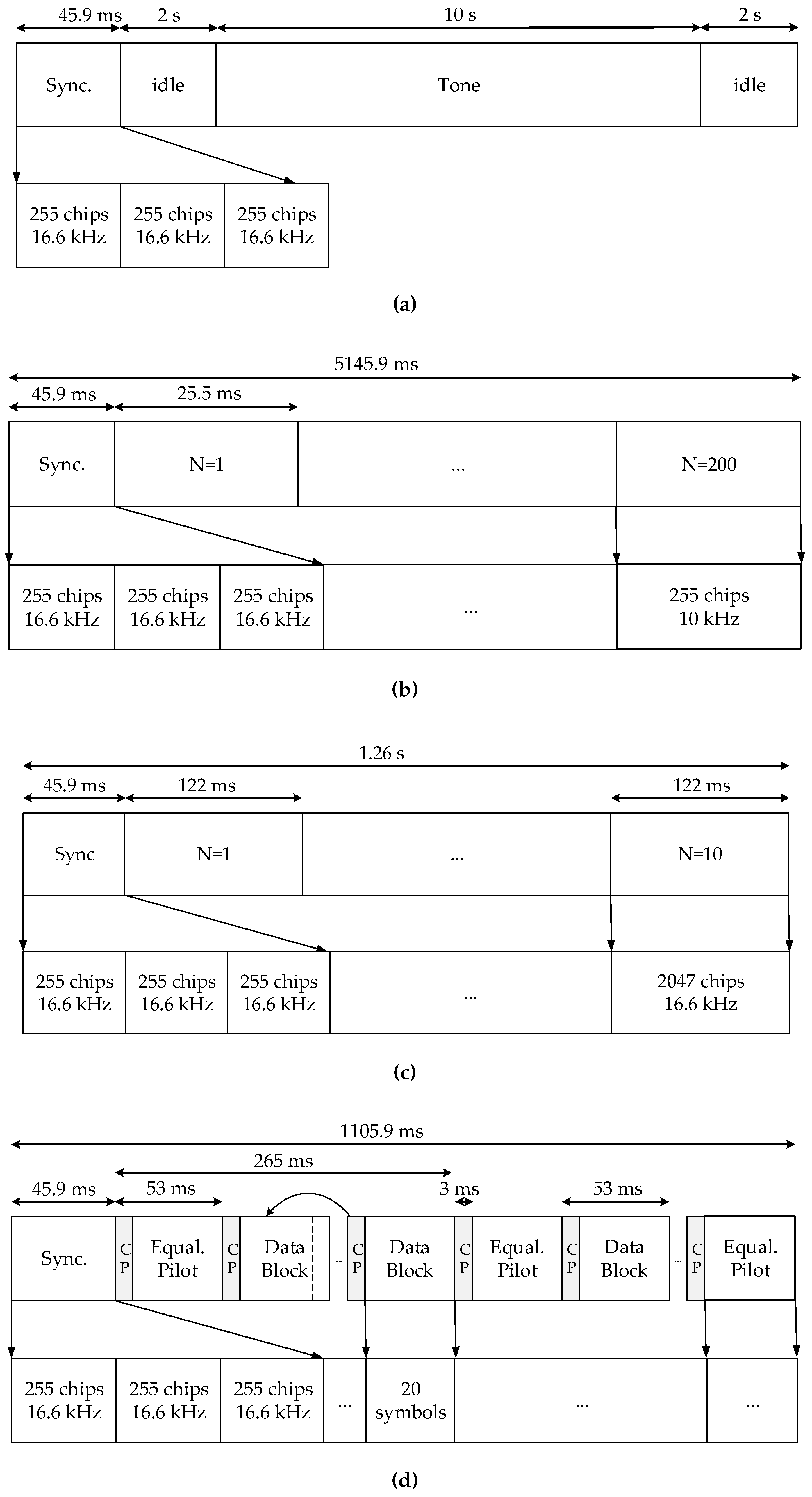
Four different frame structures are defined to satisfy the needs of the physical layer definition of the remote sensing sounder: (i) a frame for narrowband sounding (Figure 12a); (ii) a frame for wideband sounding (Figure 12b); (iii) a frame for High Robustness Mode (HRM) data transmission (Figure 12c) and (iv) a frame for High Throughput Mode (HTM) data transmission (Figure 12d).

5.3.1. Sounding Frame Structure

The narrowband sounding frame (see Figure 12a) starts with a synchronization word, in this case, a PN m-sequence of 255 chips, as described in [30], with an upfactor of 6 samples/chip, as used in [8,10,18]. After that, 2 s of silence followed by 10 s of narrowband tone transmission, and followed by 2 s of silence again. The idle periods of silence are used to measure the noise, and obtain a good estimation of SNR.

The wideband sounding frame (see Figure 12b) starts with the same synchronization word as the narrowband sounding, a PN m-sequence length 255 chips [30] with upfactor of 6 samples/chip. 5.1 s of wideband data is transmitted, using a PN m-sequence of 255 chips of type m [28,29] with an upfactor equal to 10 samples/chip, obtaining a total of 200 consecutive sequences with a bandwidth of 10 kHz. This amount of data allows the system to work with the channel response matrix and, afterwards, with the scattering function. From these two functions the delay spread and the Doppler spread of the channel will be obtained, as well as the SNR for wideband and the number of paths.

Finally, the data frame structure will vary depending on if it is working in the daytime configuration or in nighttime configuration. Despite this, as seen in Figure 12c,d, the frame starts with a synchronization part, containing three m-sequences of 255 chips with an upfactor of 6 samples/chip, using a total time of 45.9 ms of synchronization time (see Section 4.3). No channel coding or interleaving will be applied to the data, as the retransmission is the used error control (see Section 4.2).

5.3.2. Daytime

The High Robustness Mode (HRM) is defined during the daytime because it shows the worst performance in terms of SNR and availability (see previous studies in [7,12,18]). Spread Spectrum modulations are the best solution in cases of low availability and, in order to increase the throughput, instead of using plain DS-SS, Signaling Spread Spectrum modulation is proposed [8], as previously detailed in Section 4.4.1.

The chosen configuration fits Figure 12c, and consists in a synchronization triplet of PN m-sequences length 255 with an upfactor of 6 samples/chip, using 16.6 kHz of bandwidth. Each frame contains 10 symbols, m-sequences length 2047 with an upfactor of 6 samples/chip, working at 16.6 kHz. Each symbol, working with Signaling, contains 11 bits of information. So, each frame lasts 1.26 s and contains 110 bits, which enables us to obtain a bitrate of real 71.4 bps taking into account the synchronization triplet (90 bps without synchronization words). This means a total of 267 kbits in an hour, taking into account the synchronization time.

No channel coding is applied in this case; the chosen modulation is robust, so if the channel is available, the probability of a good reception is high. In addition, we assume that retransmission of data will be done during the daytime.

5.3.3. Nighttime

The High Throughput Mode (HTM) is defined at night because it exhibits the best performance in terms of SNR and availability. The modulation schemes that present the best trade-off between bitrate against BER are SC-FDE and the clipped version of SC-FDMA. These schemes outperform the OFDM studied previously in [9]. SC-FDE and the clipped version of SC-FDMA tested in [10,18] present similar results in terms of bitrate and BER. However, the computational cost of SC-FDMA is higher than SC-FDE due to the extra FFT (Fast Fourier Transform) and the IFFT (Inverse Fast Fourier Transform) required in both the transmitter and the receiver of SC-FDMA. For this reason, the proposed modulation scheme for high throughput mode is SC-FDE.

The chosen configuration fits Figure 12d. Each frame contains a synchronization triplet of PN m-sequences of 255 chips with an upfactor of 6 samples/chip, using 16.6 kHz of bandwidth. An equalization sequence of 50 ms is included every 265 ms, i.e., the equalization sequence is followed of 4 data blocks. Every data block contains 20 PSK symbols. Both equalization and data blocks contain a Cyclic Prefix (CP) of 3 ms. This configuration lets us obtain a bitrate of 289.357 bps allowing us to transmit 1.0417 Mb in an hour, taking into account the synchronization, equalization and CP intervals.

6. Conclusions

In this paper, the physical layer for a long-haul HF ionospheric link is presented. After years of sounding and conducting modulation tests during antarctic campaigns, the frequencies that show the best availability for each hour have been selected to transmit data in optimum conditions, taking into account the narrowband and wideband sounding, and the delay and Doppler spread measured in the wideband sounding. This part of the study led us to separate the channel performance into daytime and nighttime, depending on the frequency of large availability in every moment.

After the frequency selection, and assuming the different performance of the day and the night, spread spectrum techniques, multi-carrier and single carrier techniques were evaluated in terms of throughput and BER. This study allowed us to choose the best modulation for day and nighttime.

We identified four different situations where the HF modem may have to perform: (i) narrowband sounding; (ii) wideband sounding; (iii) daytime data transmission (HRM); and (iv) nighttime data transmission (HTM). For each of the situations the frame design has been detailed, given the previously studied results.

The HRM reaches throughputs of 267 kbits/h, while the HTM reaches more than 1 Mbit/h. Assuming that the data files are kbytes, both configurations satisfy the requirements. Retransmission is always assumed the method to guarantee a good reception, as the channel is very hostile and the communication is simplex. Despite that, in the future, several channel-coding algorithms will be tested in order to improve the BER at the receiver, specially designed for HRM and HTM modes. The presented definition of the physical layer allows us to conduct tests and measures with four frame structures, closing the radiomodem design and test. Far from closing the research in long haul ionospheric propagation, we do consider to widen the tests using other modulation techniques not considered in this study, such as frequency hopping or FSK modulation schemes, in order to compare their robustness and throughput with the present physical layer results.

With this physical layer definition, the research group finishes the design of the HF modem for the 12,700 km link from Antarctica to Spain, serving both the transmission of the Antarctic sensor data of the ASJI and the measurement of data itself as sensors for this hostile channel. The long-haul HF radio link can become an important part of the Antarctic observation systems as a remote sensing method, and serve as an alternative to satellite in real-time transmitting data collected with other environmental sensors [33].

References

- Keller, H.; Salzwedel, H.; Schorcht, G.; Zerbe, V. Geometric aspects of polar and near polar circular orbits for the use of ISLs for global communication. In Proceedings of the IEEE 48th Vehicular Technology Conference (VTC98), Ottawa, ON, Canada, 18–21 May 1998; Volume 1, pp. 199–203.
- Mortari, D.; de Sanctis, M.; Lucente, M. Design of flower constellations for telecommunication services. Proc. IEEE 2011, 99, 2008–2019. [Google Scholar]
- Pijoan, J.L.; Altadill, D.; Torta, J.M.; Alsina-Pagès, R.M.; Marsal, S.; Badia, D. Remote geophysical observatory in Antarctica with HF data transmission: A Review. Remote Sens. 2014, 6, 7233–7259. [Google Scholar] [CrossRef]
- US Department of Defense. MIL-STD-188-110A, Military Standard: Interoperability and Performance Standards for Data Modems; US Defense: Arlington County, VA, USA, 1991.
- NATO. STANAG 4415, Characteristics of a Robust, Non-Hopping, Serial-Tone Modulator/Demodulator for Severely Degraded HF Radio Links, 1st ed.; NATO Standardization Office (NSO): Brussels, Belgium, 1999. [Google Scholar]
- Vilella, C.; Miralles, D.; Pijoan, J.L. An Antarctica-to-Spain HF ionospheric radio link: Sounding results. Radio Sci. 2008, 43, 1–17. [Google Scholar] [CrossRef]
- Hervás, M.; Alsina-Pagès, R.M.; Orga, F.; Altadill, D.; Pijoan, J.L.; Badia, D. Narrowband and wideband channel sounding of an Antarctica to Spain ionospheric radio link. Remote Sens. 2015, 7, 11712–11730. [Google Scholar] [CrossRef]
- Alsina-Pagès, R.M.; Salvador, M.; Hervás, M.; Bergadà, P.; Pijoan, J.L.; Badia, D. Spread spectrum high performance techniques for a long haul high frequency link. IET Commun. 2015, 9, 1048–1053. [Google Scholar] [CrossRef]
- Bergadà, P.; Alsina-Pagès, R.M.; Pijoan, J.L.; Salvador, M.; Regué, J.R.; Badia, D.; Graells, S. Digital transmission techniques for a long haul hf link: DS-SS vs. OFDM. Radio Sci. 2014, 49, 518–530. [Google Scholar] [CrossRef]
- Hervás, M.; Alsina-Pagès, R.M.; Pijoan, J.L.; Salvador, M.; Badia, D. Advanced modulation schemes for an Antarctic long haul hf link. Telecommun. Syst. 2015. [Google Scholar] [CrossRef]
- Ads, A.G.; Bergadà, P.; Vilella, C.; Regué, J.R.; Pijoan, J.L.; Bardají, R.; Mauricio, J. A comprehensive sounding of the Ionospheric HF Radio Link from Antarctica to Spain. Radio Sci. 2013, 48, 1–12. [Google Scholar] [CrossRef]
- Davies, K. Ionospheric Radio; IET, Peter Peregrinus: Herts, UK, 1990; Volume 31. [Google Scholar]
- Bergadà, P.; Deumal, M.; Vilella, C.; Regué, J.R.; Altadill, D.; Marsal, S. Remote sensing and skywave digital communication from Antarctica. Sensors 2009, 9, 10136–10157. [Google Scholar] [CrossRef] [PubMed]
- Zuccheretti, E.; Bianchi, C.; Sciacca, U.; Tutone, G.; Arokiasamy, J. The new AIS-INGV Digital Ionosonde. Ann. Geophys. 2003, 46, 647–659. [Google Scholar]
- Marsal, S.; Torta, J.M.; Solé, J.G.; Segarra, A.; Cid, O.; Ibáñez, M.; Altadill, D. Livingston Island Geomagnetic Observations 2012 and 2012–2013 Survey. Available online: http://www.obsebre.es/images/oeb/pdfs/es/BoletinesMagnetismo/livingston_2012.pdf (accessed on 2 September 2015).
- Marsal, S.; Torta, J.M.; Riddick, J.C. An Assessment of the BGS δDδI Vector Magnetometer. Publ. Inst. Geophys. Pol. Acad. Sci. 2007, 99, 158–165. [Google Scholar]
- Marsal, S.; Torta, J.M. An evaluation of the uncertainty associated with the measurement of the geomagnetic field with a D/I fluxgate theodolite. Meas. Sci. Technol. 2007, 18. [Google Scholar] [CrossRef]
- Hervás, M.; Pijoan, J.L.; Alsina-Pagès, R.M.; Salvador, M.; Badia, D. Single-Carrier frequency domain equalization proposal for very Long Haul HF Radio Links. Electron. Lett. 2014, 17, 1252–1254. [Google Scholar] [CrossRef]
- EZNEC Antenna Software by W7EL. Available online: www.eznec.com (accessed on 19 April 2016).
- NEC Based Antenna Modeler and Optimizer. Available online: http://www.qsl.net/4nec2 (accessed on 19 April 2016).
- Burke, Ge.; Poggio, A. NEC Part I: Program Description—Theory (PDF) (Technical Report); Lawrence Livermore Laboratory: Livermore, CA, USA, 1981. [Google Scholar]
- Kurokawa, K. Power Waves and the Scattering Matrix. IEEE Trans. Microw. Theory Tech. 1965, 13, 194–202. [Google Scholar] [CrossRef]
- Ads, A.G.; Bergadà, P.; Regué, J.R.; Alsina-Pages, R.M.; Pijoan, J.L.; Altadill, D.; Badia, D. Vertical and oblique ionospheric soundings over the Long Haul HF Link between Antarctica and Spain. Radio Sci. 2015. [Google Scholar] [CrossRef]
- Perkiomaki, J. HF Propagation Prediction and Ionospheric Communications Analysis. Available online: http://www.voacap.com (accessed on 1 December 2015).
- Rappaport, T.S. Wireless Communications: Principles and Practice, 2nd ed.; Prentice Hall: Englewool Cliffs, NJ, USA, 2002. [Google Scholar]
- Deumal, M.; Vilella, C.; Socoro, J.; Alsina-Pagès, R.M.; Pijoan, J.L. A DS-SS signaling based system proposal for low SNR HF digital communications. In Proceedings of the 10th International Conference on Ionospheric Radio Systems and Techniques, London, UK, 18–21 July 2006; pp. 128–132.
- Proakis, J. Digital Communications, 4th ed.; McGraw Hill: Boston, MA, USA, 2000. [Google Scholar]
- Gold, R. Maximal recursive sequences with 3-valued recursive cross-correlation functions. IEEE Trans. Inf. Theory 1968, 14, 154–156. [Google Scholar] [CrossRef]
- Sarwate, D.V.; Pursley, M.B. Crosscorrelation properties of pseudorandom and related sequences. Proc. IEEE 1980, 68, 593–619. [Google Scholar] [CrossRef]
- Golomb, S. Shift Register Sequences; Holden-Day: San Francisco, CA, USA, 1967. [Google Scholar]
- Milewski, A. Periodic sequences with optimal properties for channel estimation and fast start-up equalization. IBM J. Res. Dev. 1983, 27, 426–431. [Google Scholar] [CrossRef]
- Jiang, T.; Wu, Y. An overview: Peak-to-average power ratio reduction techniques for OFDMA signals. IEEE Trans. Broadcast. 2008, 54, 257–268. [Google Scholar] [CrossRef]
- Liu, Y.; Kerkering, H.; Weisberg, R.H. Coastal Ocean Observing Systems; ISBN 978-0-12-802022-7. Elsevier: London, UK, 2015; p. 461. [Google Scholar]
© 2016 by the authors; licensee MDPI, Basel, Switzerland. This article is an open access article distributed under the terms and conditions of the Creative Commons Attribution (CC-BY) license (http://creativecommons.org/licenses/by/4.0/).