Evaluation of Stray Light Correction for GOCI Remote Sensing Reflectance Using in Situ Measurements

Abstract

The Geostationary Ocean Color Imager (GOCI) is the world’s first ocean color sensor in geostationary orbit. Although the GOCI has shown excellent radiometric performance with little long-term radiometric degradation and a high signal-to-noise ratio, there are radiometric artefacts in GOCI Level 1 products caused by stray light detected within the GOCI optics. To correct the radiometric bias, we developed an image-based correction algorithm called the correction of the interslot discrepancy using the minimum noise fraction transform (CIDUM) in a previous study and evaluated its performance with respect to the physical radiometric quantity stored in Level 1 products, i.e., top-of-atmosphere radiance. This study evaluated the performance of the CIDUM algorithm in terms of remote sensing reflectance, which is one of the most important products in ocean color remote sensing. The resultant CIDUM-corrected remote sensing reflectance products were validated using both relative (within the image) and absolute references (in situ measurements). Image validation showed that CIDUM corrected the bias in remote sensing reflectance (up to 20%) and reduced the bias to ≤5% in the tested image. In situ validation showed that relative uncertainty was reduced by around 10% within the visible bands and the correlation between the in situ and GOCI radiometric data was enhanced.

1. Introduction

The Geostationary Ocean Color Imager (GOCI) was launched in June 2010 and has produced regional-scale ocean color data over areas of East Asia around the Korean Peninsula [1,2]. GOCI acquires images of the target area (2500 × 2500 km area; centered at 36°N, 130°E) through the “step-and-stare” method, where the entire target area is subdivided into 16 (4 × 4) areas, each of which is sequentially covered by a single 2-dimensional CMOS detector [3]. In the sequential acquisition, the area or portion covered by the single acquisition is referred to as a “slot”. Radiometric data for each slot is stored in a Level 1A (L1A) file and the images for all the slots are later combined into a mosaicked image (Level 1B (L1B) data) of the entire target area through re-projection to the GOCI orthogonal map projection.

Ideally, boundary areas between adjacent slots should not exhibit any systematic radiometric discontinuity other than that created by natural variability. This is induced mainly through differences in image acquisition times and it usually does not exceed 3% in the normalized top-of-atmosphere (TOA) radiance [4]. However, previous experiments [4] have shown that strong interslot radiometric discrepancy (ISRD) of up to 20% exists in the normalized TOA radiance in the red (680 nm) and near-infrared (NIR) (865 nm) bands for slot pairs with N–S alignment. The requirement of radiometric uncertainty for the visible to NIR bands of earth observing satellites is usually ~2% and there are stricter requirements for ocean color sensors. Thus, an ISRD of 20% is an extraordinarily large bias that could jeopardize the atmospheric correction procedure. Moreover, radiometric bias causes significant problems in the algorithms that use information from the spectral bands that are affected by ISRD (e.g., the fluorescence line height method for estimating chlorophyll concentration).

One of the major artificial sources of ISRD is stray light that occurs within the sensor optics. A ray-tracing simulation [5] demonstrated that stray light from various optical paths within the GOCI sensor optics could generate radiometric inflation, particularly for the lower parts of each slot. We refer to the radiometric anomaly caused by stray light within the sensor optics as stray-light-driven radiometric inflation (SLRI). Naturally, the existence of SLRI in one slot creates ISRD between adjacent slots. The intensity of SLRI depends on both the location and the reflectivity of bright targets near the target area (mostly from northern parts of the target point), making the spatiotemporal pattern of SLRI variability dependent on the surrounding environment.

To mitigate the degree of SLRI in GOCI L1B images, we proposed an image-based correction algorithm called the correction of inter-slot radiometric discrepancy using the minimum noise fraction transform (CIDUM) [4]. The CIDUM algorithm comprises three steps. (1) First, the spatial distribution of SLRI is identified in individual slots using the minimum noise fraction (MNF) transform [6]; (2) Then, the extracted pattern is scaled to the actual SLRI using the pixels in the slot overlaps; (3) Finally, the estimated SLRI is subtracted from the original L1A image. CIDUM recovers the discontinuity in the slot boundaries in L1B data (TOA radiance) successfully, reducing the large SLRI that can reach up to 20% to less than 3% in all the slot boundaries of the tested GOCI data sets [4].

In this study, we performed further validation on the CIDUM algorithm, focusing particularly on the quality of remote sensing reflectance ($R_{rs}$) that is derived from the atmospheric correction process. Remote sensing reflectance is an important product in ocean color remote sensing because it plays a critical role in the estimation of the concentrations of optically active water constituents such as chlorophyll pigment concentration, suspended sediment concentrations, and dissolved organic matter. The impact of the CIDUM correction on $R_{rs}$ data is not as straightforward as in TOA radiance data. The atmospheric correction process is a nonlinear process that involves an iterative aerosol-estimation procedure, in which a positive bias in TOA radiance does not necessarily induce a positive bias in remote sensing reflectance. Furthermore, the relative portion of SLRI is greater in the Rayleigh-corrected radiance than in TOA radiance, making the aerosol-estimation process based on band ratios more sensitive to SLRI.

Two approaches were adopted to validate the results in $R_{rs}$. In the first approach, improvements in $R_{rs}$ after the application of CIDUM were quantified at the slot boundary by comparing the $R_{rs}$ of nearby pixels from different slots. A ray-tracing simulation [5] has shown that the upper part of a slot is affected little by SLRI, allowing those boundary areas beneath the slot boundary to be used as the reference spectrum for the assessment of the results of the correction in the upper slot. Although there is a difference between the acquisition times of the two slots, comparison of both the corrected and the uncorrected data with the reference data can provide insight into the correction quality. The second approach used an absolute validation based on independent in situ radiometric measurements. Whereas the first approach (hereafter, referred to as “boundary analysis”) evaluated the relative performance of the correction within the restricted area (feasible only near the slot boundary), the second approach evaluated the absolute performance of the correction, including those areas far from the slot boundary.

2. Materials and Methods

2.1. CIDUM Algorithm with Minor Modification

For the validation in this study, a slight modification was applied to the previously proposed CIDUM algorithm [4] to improve the removal of SLRI from the data. Previously, in the original proposal, the SLRI pattern extracted from the MNF transform was scaled based on the radiometric differences of the slot overlaps after normalization to the sun elevation angle, i.e., the normalized TOA radiance. However, the sun elevation angle differs for the different slots causing variation in the level of Rayleigh scattering, which increases the uncertainty in the comparison of the TOA radiances in the slot overlaps. In the modified CIDUM, pixels in the slot overlaps were compared in terms of Rayleigh-corrected reflectance rather than normalized TOA radiance.

Here, we provide a brief description of the modified CIDUM algorithm. CIDUM utilizes the MNF transform for the extraction of the SLRI pattern from individual L1A images. The MNF transform is efficient in detecting image artefacts that have strong spatial autocorrelation. For example, the smile effect in Hyperion data, which causes a gradual alteration of the measured radiance in marginal areas of images with a wide angle of view was identified and corrected using the MNF transform [7]. Formulation of the MNF transform was presented in Appendix.

The SLRI patterns extracted from the L1A images are calibrated against the adjacent slots in such a way that the mean statistics of the pixels in the overlapped region are equalized. Specifically, for a pair of slots, the mean Rayleigh-corrected reflectances are supposed equal if there is no SLRI effect, i.e.,:

$${\rho }_{rc}^{\left(1\right)}={\rho }_{rc}^{\left(2\right)}$$

(1)

where ${\rho }_{rc}^{\left(i\right)}$ denotes the Rayleigh-corrected reflectance in the i-th slot. The value of ${\rho }_{rc}^{\left(i\right)}$ is calculated from the TOA radiance ($L_{TOA}^{\left(i\right)}$) as follows:

$${\rho }_{rc}^{\left(i\right)}={\rho }_{TOA}^{\left(i\right)}-{\rho }_r^{\left(i\right)}$$

(2)

$$=\frac{\pi L_{TOA}^{\left(i\right)}}{\cos {\theta }_s^{\left(i\right)}{F}_0^{\left(i\right)}}-{\rho }_r^{\left(i\right)}$$

(3)

where ${\rho }_{TOA}^{\left(i\right)}$ is the TOA reflectance, ${\theta }_s^{\left(i\right)}$ is the solar zenith angle, and ${\rho }_r^{\left(i\right)}$ is the Rayleigh reflectance computed using the 6S code [8]. The unbiased TOA radiance ($L_{TOA}^{\left(i\right)}$) is computed by subtracting the SLRI radiance ($L_{SLRI}^{\left(i\right)}$) from the observed at-sensor radiance ($L_{obs}^{\left(i\right)}$) as

$$L_{TOA}^{\left(i\right)}=L_{obs}^{\left(i\right)}-L_{SLRI}^{\left(i\right)}$$

(4)

If we define $k^{\left(i\right)}$ as

$$k^{\left(i\right)}=\frac{\pi }{\cos {\theta }_s^{\left(i\right)}{F}_0^{\left(i\right)}}$$

(5)

where $F_0$ is the solar irradiance, then Equation (1) can be formulated in terms of the known variables ($L_{obs}^{\left(i\right)}$, $k^{\left(i\right)}$, and ${\rho }_r^{\left(i\right)}$) and the unknown variables ($L_{SLRI}^{\left(i\right)}$) as:

$$k^{\left(1\right)}\left(L_{obs}^{\left(1\right)}-L_{SLRI}^{\left(1\right)}\right)-{\rho }_r^{\left(1\right)}=k^{\left(2\right)}\left(L_{obs}^{\left(2\right)}-L_{SLRI}^{\left(2\right)}\right)-{\rho }_r^{\left(2\right)}$$

(6)

$$\left[k^{\left(1\right)}{L}_{obs}^{\left(1\right)}-{\rho }_r^{\left(1\right)}\right]-\left[k^{\left(2\right)}{L}_{obs}^{\left(2\right)}-{\rho }_r^{\left(2\right)}\right]=k^{\left(1\right)}{L}_{SLRI}^{\left(1\right)}-k^{\left(2\right)}{L}_{SLRI}^{\left(2\right)}$$

(7)

The SLRI radiance ($L_{SLRI}^{\left(i\right)}$) is computed from the MNF transform after applying the slot-dependent calibration factor ${\alpha }^{\left(i\right)}$:

$$L_{SLRI}^{\left(i\right)}={\alpha }^{\left(i\right)}{X}_{MNF}^{\left(i\right)}$$

(8)

where $X_{MNF}^{\left(i\right)}$ is the SLRI signal image extracted from the MNF transform. Now, constructing the equations for all 24 slot pairs generates the linear system that has 16 unknowns (calibration factors for 16 slots) and 24 constraints. Solving the linear system provides an optimal set of calibration factors that minimizes the overall ISRD between all the slot pairs.

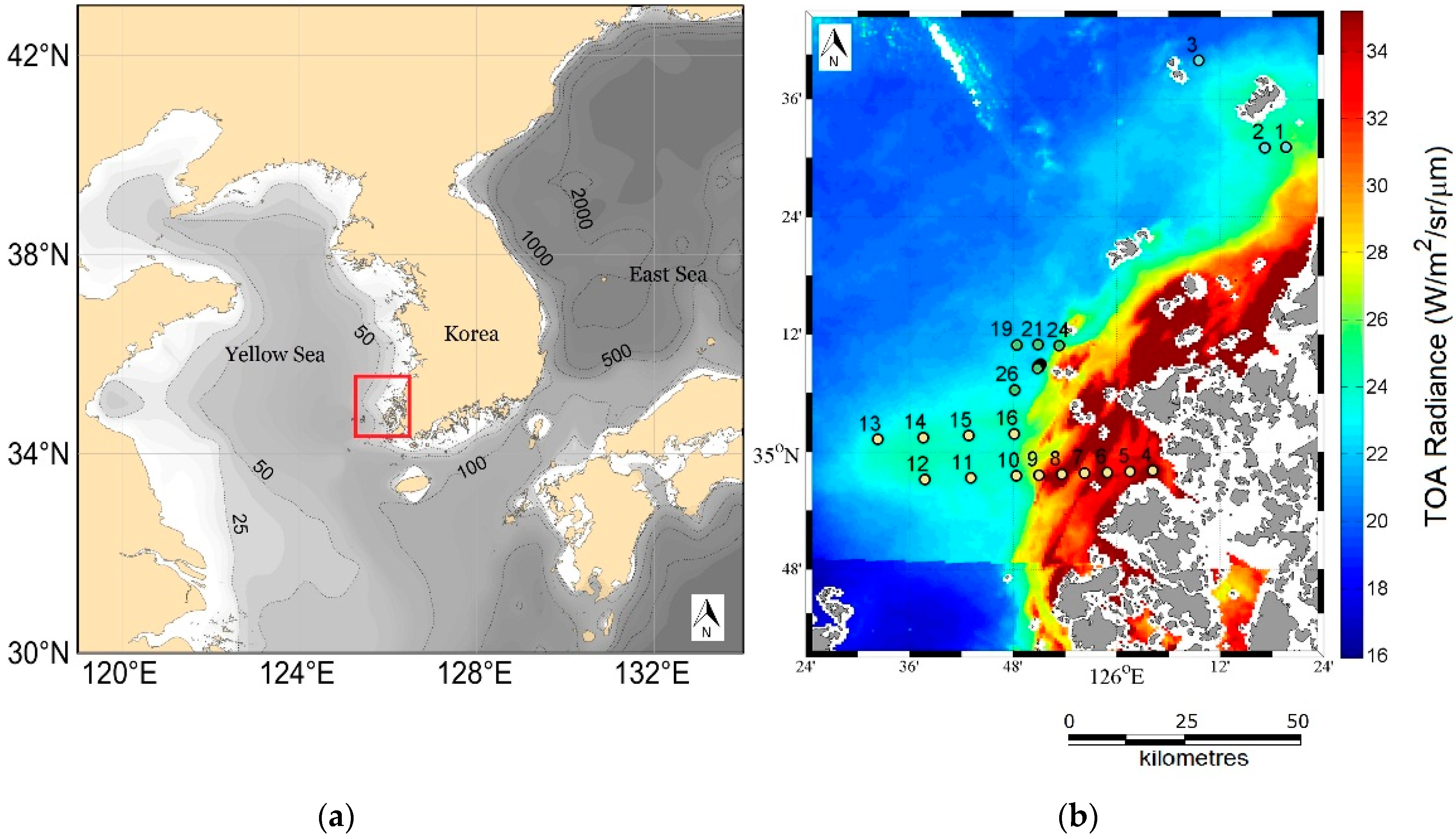
2.2. Study Area and Field Measurements

For an independent evaluation of the algorithm, above-water radiometric measurements were acquired off the west coast of Korea using the ASD^® and TriOS^® hyperspectral radiometers. After a quality control process that screened the in situ measurements for poor-quality data [9], 26 match-up pairs between the in situ and the GOCI $R_{rs}$ were identified in the GOCI data over three days (31 July 2012, 16 October 2012, and 23 October 2013), which are dates that had strong SLRI in the corresponding L1B images. Since GOCI images were taken every hour, the maximum time difference between in situ measurements and the corresponding GOCI data is 30 min if the in situ data were collected between 00:16 UTC and 07:46 UTC. This study used the GOCI Data Processing System (GDPS) atmospheric correction process (version 1.31) [10].

The locations of the 26 measurement stations are displayed in Figure 1 with the background image of $L_{TOA}\left(680\right)$ acquired on 31 July 2012 (UTC 02). This area has large spatiotemporal variability in $R_{rs}$, which is dominated by the variation in suspended sediment concentration. Resuspension from tidal movement in the shallow water and the existence of a mud belt (Heuksan mud belt) in the offshore area cause high concentrations of suspended sediment of 10–100 g/m³. The acquisition times and the geographic coordinates of the in situ data are presented in

Table 1. Times and locations of the 26 in situ radiometric measurements used for this study. Time is in Coordinated Universal Time (UTC).

ID	Year	Month	Day	Latitude	Longitude	Hour	Minute
1	2012	07	31	35.5179	126.3264	02	04
2				35.5178	126.2855	02	23
3				35.6653	126.1580	05	10
4	2012	10	16	34.9686	126.0695	00	10
5				34.9671	126.0255	00	28
6				34.9656	125.9816	00	47
7				34.9642	125.9377	01	04
8				34.9626	125.8938	01	24
9				34.9611	125.8498	01	40
10				34.9596	125.8059	02	02
11				34.9564	125.7180	02	40
12				34.9533	125.6302	03	02
13				35.0219	125.5384	04	27
14				35.0251	125.6263	04	54
15				35.0283	125.7143	05	21
16				35.0315	125.8022	05	48
17	2013	10	23	35.1479	125.8511	00	20
18				35.1497	125.8528	01	25
19				35.1826	125.8072	01	58
20				35.1465	125.8483	02	27
21				35.1830	125.8476	02	52
22				35.1477	125.8503	03	22
23				35.1442	125.8495	04	27
24				35.1811	125.8887	04	52
25				35.1425	125.8474	06	23
26				35.1061	125.8036	06	53

for the 26 stations used in the validation.

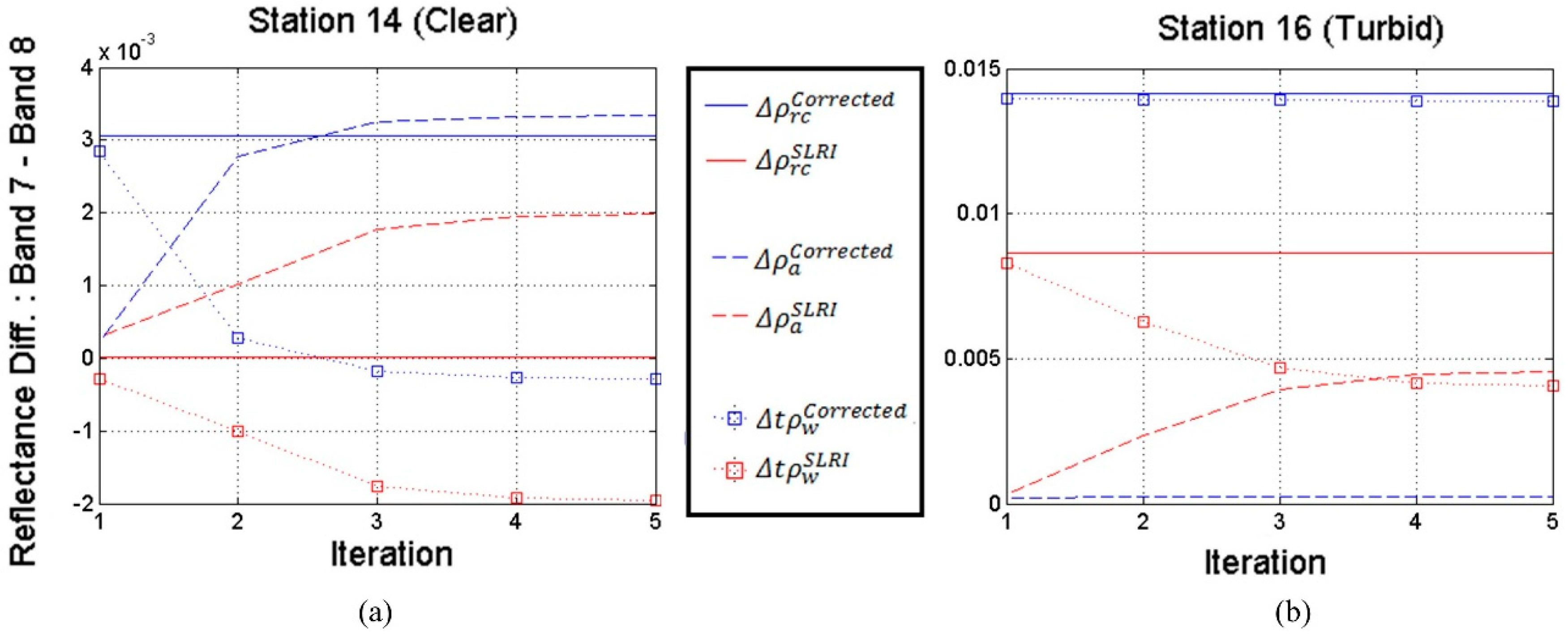
2.3. Aerosol Estimation Process for Turbid Waters

To analyze the effect of the stray light in the course of atmospheric correction, it is necessary to observe how the radiometric artefact propagates during the aerosol estimation process which is typically initiated in turbid waters. The iterative process of aerosol estimation embedded in the GDPS 1.3 atmospheric correction [9,11], is described briefly in the following.

• (Step 1) Estimating aerosol reflectance in the NIR bands (745 and 865 nm) 

Under a given reflectance budget of Rayleigh-corrected reflectance (${\rho }_a$), the aerosol reflectance is obtained by subtracting $t {\rho }_w$ from ${\rho }_{rc}$ as in

$${\rho }_a\left(NIR\right)\leftarrow {\rho }_{rc}\left(\text{NIR}\right)-t{\rho }_w\left(NIR\right)$$

(9)

The water reflectance in the NIR bands is assumed zero at the first iteration; however, it will have non-zero values for turbid water as the iteration progresses.

$${\rho }_w\left(NIR\right)=0 \left(\text{at the first iteration}\right)$$

(10)

• (Step 2) Selecting the aerosol models and estimating aerosol reflectance 

Based on the multiple-scattering $\mathsf{\epsilon }$, defined as

$$\mathsf{\epsilon }=\frac{{\rho }_a\left(745\right)}{{\rho }_a\left(865\right)}$$

(11)

the most probable aerosol models and their weightings are computed using the look-up table that relates multiple-scattering $\mathsf{\epsilon }$ with single-scattering $\mathsf{\epsilon }$.

• (Step 3) Updating $\mathit{t} {\mathit{\rho }}_{\mathit{w}}$ for the visible bands 

Now that the aerosol reflectances for the visible bands (${\rho }_a\left(VIS\right)$) are available, following Step 2, the water reflectance at 660 nm is updated as in

$$t{\rho }_w\left(660\right) \leftarrow {\rho }_{rc}\left(660\right)-{\rho }_a\left(660\right)$$

(12)

• (Step 4) Estimating water reflectance at the NIR bands 

According to the water reflectance model in the NIR wavelength region [12], the ${\rho }_w$ of the NIR bands have a monotonic relationship with ${\rho }_w\left(660\right)$ formulated by a fourth-order polynomial.

$${\rho }_w\left(745\right), {\rho }_w\left(865\right)=f\left({\rho }_w\left(660\right)\right)$$

(13)

The water reflectances of the NIR bands are determined based on Equation (13).

• (Step 5) Repeating Steps 1 through 4 until convergence 

In the process, Steps 1 through 4 are repeated until ${\rho }_a$ and ${\rho }_w$ at a certain run have no significant changes compared with the previous iteration.

3. Results

As briefly mentioned in Introduction, CIDUM results are assessed with two approaches: (1) boundary analysis; and (2) in situ analysis. In the boundary analysis (Section 3.1), remote sensing reflectance data near a slot boundary are compared between an original image and the CIDUM-corrected image, where the differences in the atmospheric correction results are quantified in terms of Rayleigh-corrected, aerosol, and remote sensing reflectance. In the in situ analysis (Section 3.2), the changes in the reflectance variables before and after the CIDUM algorithm are assessed using in situ radiometric measurements, which are available not only in the slot boundary area but also in remote areas from the boundary.

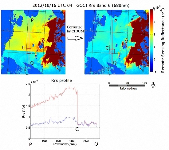
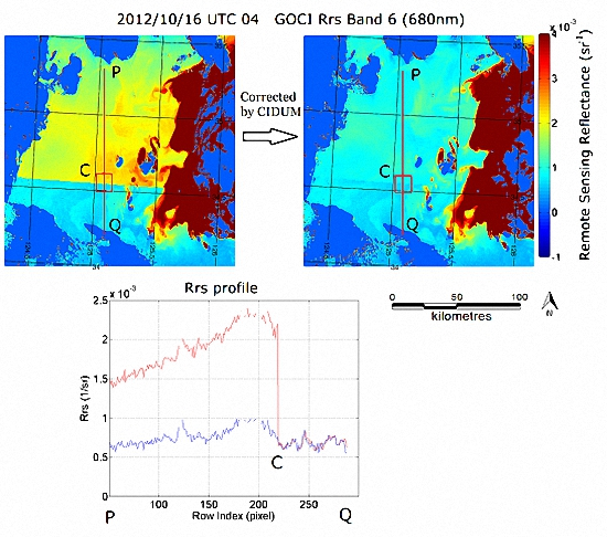
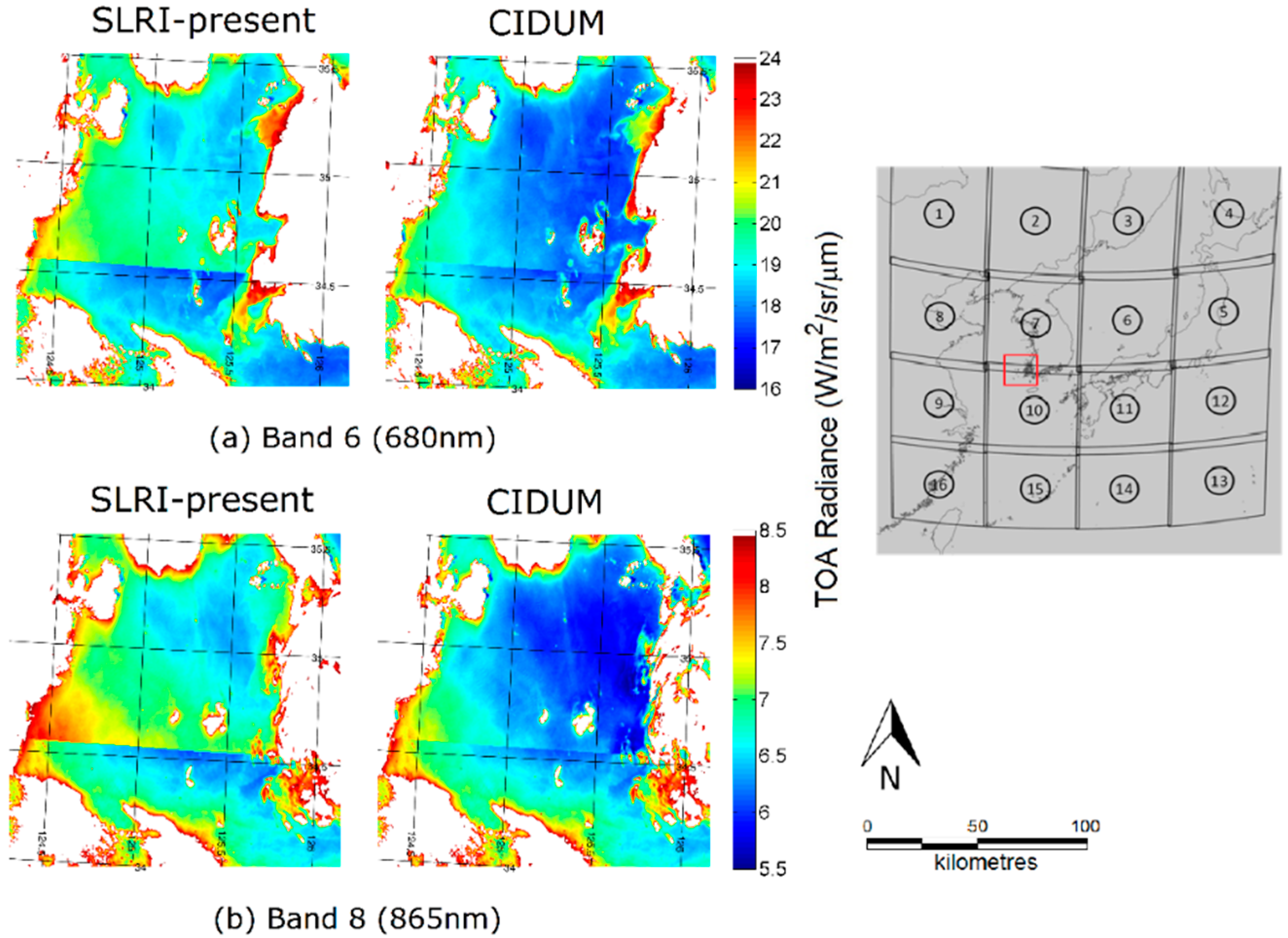
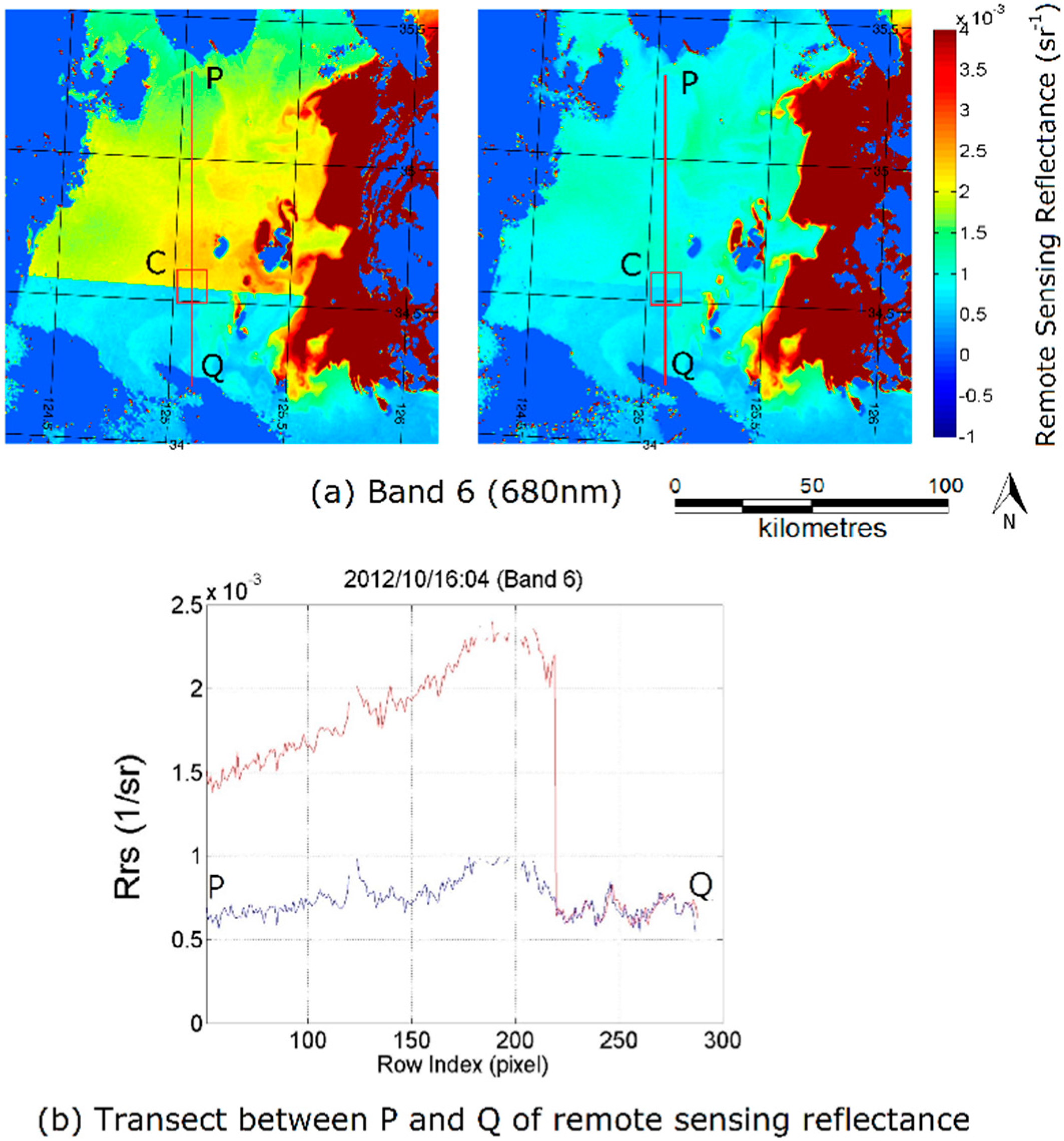
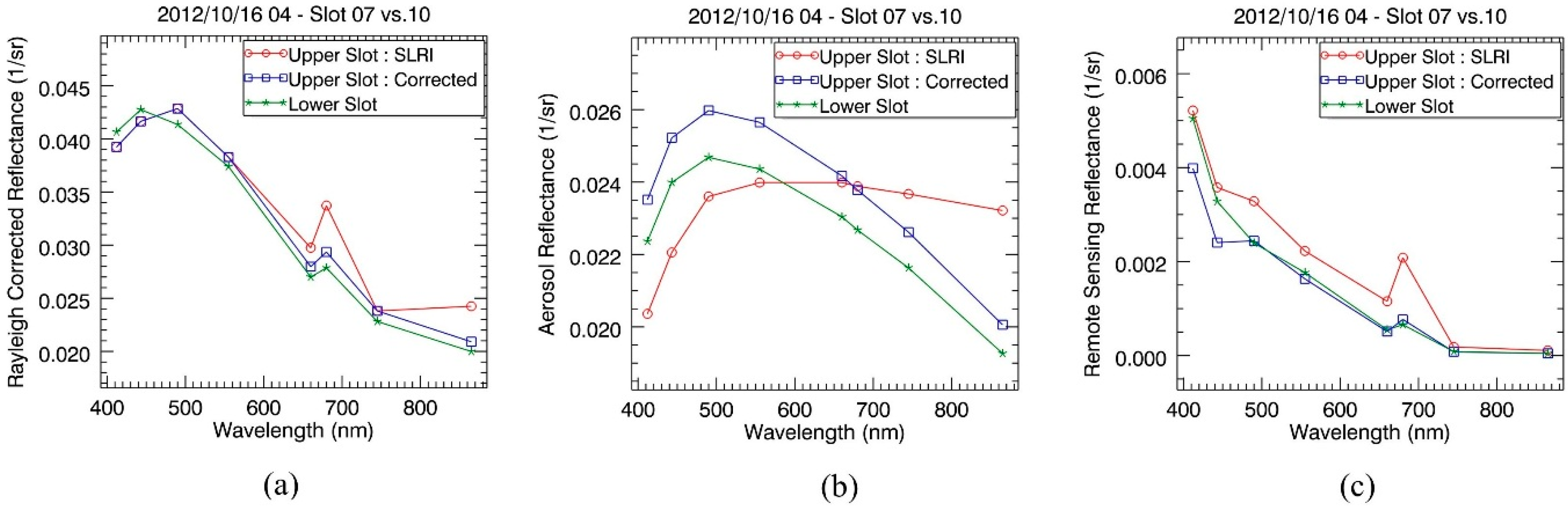
3.1. Boundary Analysis

Before analyzing the results in $R_{rs}$, the correction results in the TOA radiance (L1B) data are first shown in Figure 2. Figure 2 shows images of TOA radiance both before and after the CIDUM correction: Band 6 ($L_{TOA}\left(680\right)$) in Figure 2a and Band 8 ($L_{TOA}\left(865\right)$) in Figure 2b. The color scales of the figures are adjusted to the areas of the ocean that are relatively clear, which makes high-reflectance targets such as clouds, high concentrations of aerosols, land areas, and ocean areas of high turbidity have saturated values (white). In both spectral bands, the discontinuity across the slot boundary between Slot 7 (upper slot) and Slot 10 (lower slot) is shown mitigated in the corrected images (right), recovering the continuity of the natural variability. Note that a certain amount of discontinuity is unavoidable because of the difference in acquisition time between the upper and lower slots (the difference in acquisition time between Slots 7 and 10 is around 5 min). To assess the improvement achieved by the correction, the ISRD is measured in terms of the relative mean difference (ψ) of the Rayleigh-corrected reflectance (${\rho }_{rc}$) between the pixels in the slot overlaps:

$${\mathsf{\psi }}_{\rho rc}={\displaystyle \sum }_i^N\frac{{\rho }_{rc}{}^{\left(upperslot\right)}-{\rho }_{rc}{}^{\left(lowerslot\right)}}{{\rho }_{rc}{}^{\left(lowerslot\right)}}$$

(14)

where N is the total number of samples in the slot overlap used to compute the statistics. While the slot boundary with no evident SLRI had a value of ${\mathsf{\psi }}_{\rho rc}$ < 5%, according to the previous observations, this slot pair has large values of ${\mathsf{\psi }}_{\rho rc}$ of 6.9%, 15.6%, and 17.5% for Bands 5, 6, and 8, which were reduced to 2.4%, 4.9%, and 5.2%, respectively, after the correction.

Figure 3 shows the image of $R_{rs}$ for Band 6 together with the $R_{rs}$profile along transect PQ. In the figure, high-reflectance targets that are ineligible for the regular atmospheric correction algorithm (e.g., land and cloud) are filled with the lowest values of the color scale and excluded from the analysis. In the $R_{rs}$ image (Figure 3a), the effect of SLRI is clear in the upper slot (Slot 7) before the correction (left-hand figure), which induces overestimation in $R_{rs}$ (660) in the upper slot and significant discontinuity at the slot boundary. The $R_{rs}$ profile along the vertical transect between points P and Q reveals that the discontinuity at the boundary point is due to overestimation. The correction removes the overestimation from $R_{rs}$ in the upper slot (right-hand figure), while maintaining the original local variability in the profile. The $R_{rs}$ bias is largest at the bottom of the slot and it tapers off further north.

To further investigate the impact on the atmospheric correction process, reflectance spectra of the intermediate products are plotted for the pixels in a small area (Box C) at the slot boundary. The atmospheric correction process removes the reflectance contributed by Rayleigh scattering and aerosol scattering from the TOA reflectance measured at the sensor. TOA reflectance is expressed as

$${\rho }_{TOA}={\rho }_r+{\rho }_a+t_u {\rho }_w$$

(15)

$${\rho }_{rc}={\rho }_a+t_u {\rho }_w$$

(16)

where ${\rho }_a$ is aerosol reflectance, ${\rho }_{w }$is water reflectance, and $t_u$ is upward diffuse transmittance. The water reflectance is related to ${\rho }_{rs}$ through

$${\rho }_w=f t_d R_{rs}/\pi$$

(17)

where f is the coefficient for the bidirectional effect, and $t_d$ is downward diffuse transmittance. We can obtain $R_{rs}$ from ${\rho }_{TOA}$ through the atmospheric correction. The effect of CIDUM can be assessed in terms of the three intermediate reflectance products in the process: the Rayleigh-corrected reflectance (${\rho }_{rc}$), aerosol reflectance (${\rho }_a$), and remote sensing reflectance ($R_{rs}$). Figure 4 presents the mean spectra of the three types of reflectance for the pixels of box C in Figure 3. For each type of reflectance, three different data sources were used: (1) pixels in the box that belong to the upper slot before the CIDUM correction (${\rho }^{SLRI}$) (red line); (2) the same pixels as (1) but with SLRI corrected by CIDUM (${\rho }^{Corr}$) (blue line); and (3) pixels in the box that belong to the lower slot (${\rho }^{Ref}$) (green line). As mentioned earlier, because the uppermost part of the lower slot was assumed to have no SLRI, the statistics obtained from the lower slot pixels can be considered references under the assumption that the optical environment (e.g., aerosol loading and concentration of water constituents) does not vary significantly across the slots.

The ${\rho }_{rc}$ spectra (Figure 4a) show that ${\rho }_{rc}^{SLRI}$ is overestimated compared with ${\rho }_{rc}^{Corr}$ with a relative difference of 4.8%, 18.1%, and 17.3% for Bands 5, 6, and 8, respectively. The large overestimation in Band 8 (865 nm) is critical in deriving $R_{rs}$, because the aerosol model and loading for the pixel location is estimated primarily based on the ${\rho }_{rc}$ ratio of the two NIR bands (Bands 7 and 8), i.e., the multiple scattering epsilon ($\mathsf{\epsilon }$). The values of $\mathsf{\epsilon }$ before and after the correction are 3.4 and 6.5, respectively, which led to the significantly different aerosol reflectance spectrum over the GOCI spectral range, as shown in Figure 4b. The large ${\rho }_{rc}^{SLRI}\left(865\right)$ values (which consequently led to low values of $\epsilon$) caused ${\rho }_a^{SLRI}\left(865\right)$ to be greatly overestimated and made ${\rho }_a^{SLRI}$ of the visible bands (Bands 1–6) underestimated. Under the fixed total reflectance budget, the underestimation in ${\rho }_a^{SLRI}$ in turn caused the overestimation of $R_{rs}^{SLRI}$ in the corresponding spectral range, as shown in Figure 4c CIDUM successfully corrected biases in all the three GOCI reflectance estimates induced by SLRI, producing GOCI remote sensing reflectance ($R_{rs}^{Corr}$) very close to that from the reference data ($R_{rs}^{Ref}$) (relative difference of <1% in all bands except Band 1 and 2). The abrupt decreases in $R_{rs}$ in the blue bands (Bands 1 and 2) that are unique in the samples in the upper slot are due to pixel response non-uniformity, where the detectors in the marginal area of the 2-dimensional detector array have non-uniform photo responsivity for Bands 1 and 2 [13]. The slight difference between the spectra of ${\rho }_{rc}^{Corr}$ and ${\rho }_{rc}^{Ref}$ which is considered to be induced by local variability in the aerosol condition was properly explained in the aerosol reflectance in Figure 4b, which then resulted in consistent remote sensing reflectance in ocean waters.

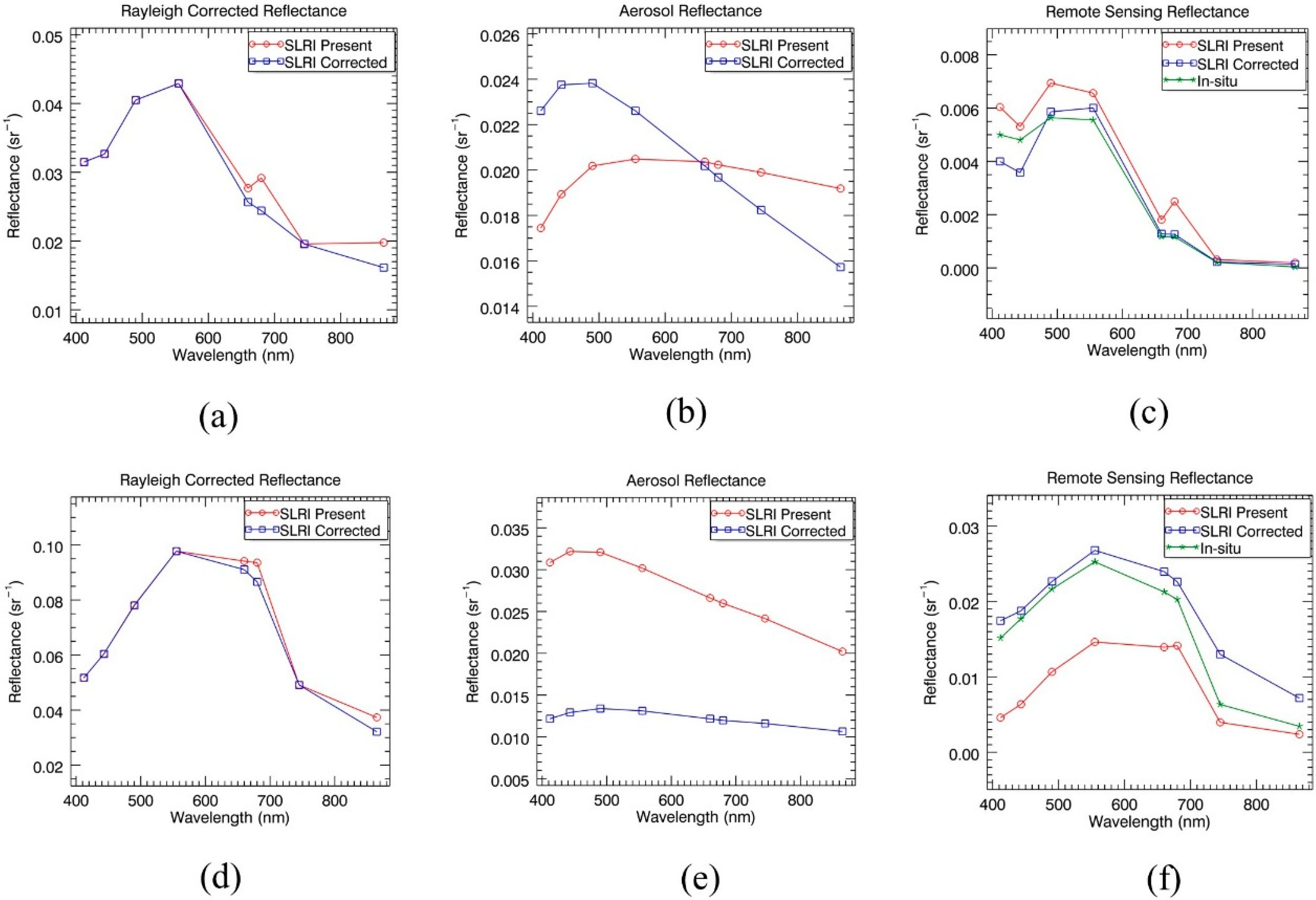
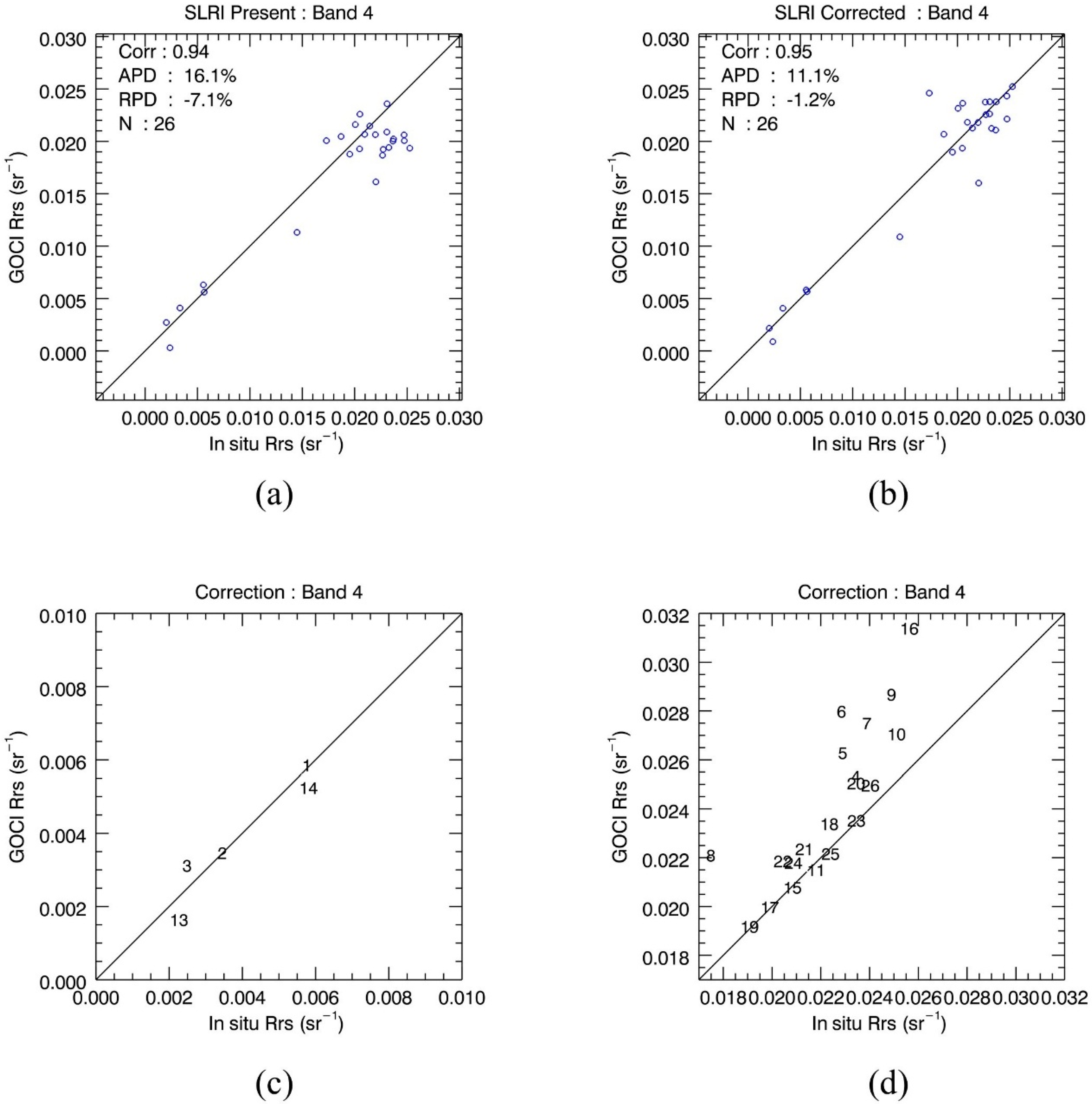
3.2. Assessment with in Situ Radiometric Measurements

In this section, the uncertainty of the GOCI $R_{rs}$ is computed using the in situ $R_{rs}$ measurements collected at the 26 stations near the slot boundary between Slots 7 and 10. For each in situ measurement, the temporally closest GOCI scene was selected and the average value of a 3 × 3 pixel window, centered at the in situ location, was compared with the in situ measurement. The maximum time difference between the GOCI and in situ data allowed in this validation was 1 h. Because of the high temporal resolution of GOCI (hourly from 09:00 to 16:00 local time), there are usually two GOCI scenes available for match-up. When multiple GOCI data were available for the match-up, the temporally closest GOCI data were used. A spatial homogeneity test was performed for the pixels in the window to verify whether the average values of the window were representative of the window area (the coefficient of variation was <5% in all the stations). Two statistics were used to evaluate the uncertainty in the resultant GOCI $R_{rs}$: the absolute mean percentage difference (APD,$\left|{\mathsf{\psi }}_{Rrs}\right|$) and the relative mean percentage difference (RPD, ${\mathsf{\psi }}_{Rrs}$), which are given as:

$$\left|{\mathsf{\psi }}_{Rrs}\right|={\displaystyle \sum }_i^N\left|\frac{R_{rs}{}^{\left(GOCI\right)}-R_{rs}{}^{\left(insitu\right)}}{R_{rs}{}^{\left(insitu\right)}}\right|$$

(18)

$${\mathsf{\psi }}_{Rrs}={\displaystyle \sum }_i^N\frac{R_{rs}{}^{\left(GOCI\right)}-R_{rs}{}^{\left(insitu\right)}}{R_{rs}{}^{\left(insitu\right)}}$$

(19)

Figure 5a,b presents scatter plots of $R_{rs}\left(555\right)$ between the GOCI and in situ data before and after the application of CIDUM, respectively. The overall data scatter (i.e., APD=$\left|{\mathsf{\psi }}_{Rrs}\right|$) was 16.1% before the correction, which was reduced to 11.1% after the correction, primarily because of the mitigated underestimation in the CIDUM-corrected data (Figure 5b), particularly for the $R_{rs}$ range of 0.02–0.025. We defined the amount of correction (Corr) as

$$Corr=R_{rs}{}^{Corr}-R_{rs}{}^{SLRI}$$

(20)

and plotted the quantity ($R_{rs}{}^{in-situ}$ + Corr) against the in situ $R_{rs}$ in Figure 5c and d (i.e., the small and large ranges of $R_{rs}$ are shown in Figure 5c,d, respectively). While Corr is relatively small for stations with $R_{rs}$(555) < 0.02 (Figure 5c), larger corrections can be observed for stations with higher $R_{rs}$(555), i.e., samples from water with greater turbidity. In Figure 5d, most of the correction was positive for samples with $R_{rs}$ (555) > 0.02 and it was greatest for the stations located closest to the slot boundary (e.g., Stations 5–7, 9, 10 and 16). The mean suspended particulate matter (SPM) concentration of these six stations is above 40 g/m³, whereas the SPM of the stations in clear water is around 1 g/m³. The largest correction was made for Station 16 (SPM = 48.65 g/m³), where Corr is ~0.006, which accounts for ~25% of the corrected $R_{rs}$ ($R_{rs}{}^{Corr}$).

Spectrum analysis was performed for two stations selected from non-turbid and turbid waters: Station 14 was in relatively clear water (SPM = 1.41 g/m³) and Station 16 was in a turbid area (SPM = 48.65 g/m³). The Rayleigh-corrected reflectance (${\rho }_{rc})$ spectra before and after the correction (Figure 6a,b) showed that the CIDUM effectively corrected the ${\rho }_{rc}$ in the SLRI-affected bands. The Corr in Bands 5, 6, and 8 was 0.0020, 0.0048, and 0.0036 for Station 14 and 0.0031, 0.0070, and 0.0052 for Station 16. Note that the correction appears smaller in the figure for Station 16 because of the different scales of the y-axes. The relative corrections against the corrected ${\rho }_{rc}$ values are 3.4%, 8.0%, and 16.2% for Station 14 and 8.0%, 19.5%, and 22.5% for Station 16 for Bands 5, 6, and 8, respectively.

Similar to the case in the previous boundary analysis, a large positive bias in ${\rho }_{rc}$(865) before the CIDUM correction induced an overestimation of the aerosol loading (i.e., high ${\rho }_a\left(865\right)$ at the both stations. At Station 14, the smaller values of $\epsilon$ ($={\rho }_{rc}\left(745\right)/{\rho }_{rc}\left(865\right))$ induced relatively flat aerosol reflectance over the entire wavelength range, which led to the underestimation of ${\rho }_a$ in the visible bands. The underestimation of ${\rho }_a$ induced an overestimation of $R_{rs}$, not only in the SLRI-affected bands but also in the other visible bands.

Contrary to the case of Station 14, the underestimated values of $\epsilon$ by SLRI for Station 16 led to greatly overestimated values of ${\rho }_a$ across the entire spectral range (red curve in Figure 6d), which led to significant underestimation of $R_{rs}$ across the entire range (red curve in Figure 6f). This opposite pattern stems from the complicated process of aerosol estimation that involves an iterative process for the separation of the aerosol and water reflectances from the Rayleigh-corrected reflectance. The discussion on the detailed mechanism is presented in Section 4.

The resultant $R_{rs}$ spectra show that the CIDUM correction generally mitigates both the overestimation and the underestimation caused by SLRI, making the GOCI $R_{rs}$ much closer to the in situ $R_{rs}$. At Station 14, the overestimation of ${\rho }_{rs}$ before the correction was 23%, 18%, 53%, and 113%, which was reduced to 4%, 8%, 8%, and 8% after the correction for Bands 3–6, respectively. The improvement was particularly significant for Band 6, which has a large impact on the estimation of the fluorescence signal from phytoplankton. The bias in the turbid water (Station 16) was −70%, −64%, −51%, −42%, −34%, and −30% before the correction, which was also greatly mitigated to 15%, 6%, 5%, 6%, 13%, and 12% for Bands 1–6, respectively.

The validation results for the other GOCI visible bands are presented in

Table 2. Match-up validation results between in situ and GOCI data before and after the CIDUM correction for the six visible bands.

	Correlation		APD ($\mathbf{\left|}{\mathsf{\psi }}_{\mathit{R}\mathit{r}\mathit{s}}\mathbf{\right|}$)		RPD (${\mathsf{\psi }}_{\mathit{R}\mathit{r}\mathit{s}}$)
	Before	After	Before	After	Before	After
Band 1	0.55	0.74	40.4	29.7	−1.4	3.1
Band 2	0.79	0.87	30.0	22.9	−13.4	−13.8
Band 3	0.90	0.92	21.3	14.2	−7.7	−4.9
Band 4	0.94	0.95	16.1	11.1	−7.1	−1.2
Band 5	0.96	0.97	37.3	27.6	−22.3	−19.1
Band 6	0.96	0.96	35.4	24.4	−3.6	−12.8

. Generally, the CIDUM improves the correlation between GOCI and in situ $R_{rs}$ and it reduces data scatter. The improvement was largest in the blue bands, where the improvement in correlation was around 0.2 and the APD improvement was nearly 10% in the 412-nm band. The improvement in bias (RPD) is band-dependent, whereby the bias is generally reduced but some bands have poorer RPDs.

4. Discussion

SLRI creates a positive bias in TOA radiance and consequently also in Rayleigh-corrected radiance/reflectance. However, in $R_{rs}$ the bias is not necessarily positive because of the complicated process of aerosol estimation in the atmospheric correction as shown in our results. A question remains regarding the specific mechanism in the iterative process that decides the sign of the bias in $R_{rs}$. To analyze the mechanism, changes in the aerosol and water reflectances in the iterative process of aerosol estimation described in Section 2.3 were tracked over five iterations at the end of the iteration.

The iterative process is basically controlled by three constraints: (1) the total reflectance budget given by ${\rho }_{rc}$, as specified in Equation (15); (2) types of aerosol models and associated aerosol loadings, determined in Step 2 in Section 2.3; and (3) water reflectance relationship between the 660-, 745-, and 865-nm bands, as specified in Equation (13). The iterative process finds the combination of ${\rho }_a$ and$t{\rho }_w$ that best fits the constraints under the reflectance budget of ${\rho }_{rc}$. Radiance data affected by SLRI will definitely produce different results from the case without SLRI in all or any of ${\rho }_{rc}$, ${\rho }_a$, and${\rho }_w$. The aim here is to investigate how the radiance bias that is created by SLRI is propagated to the reflectance products in the process of aerosol estimation. Because the impact of SLRI in the NIR bands is most critical to the atmospheric correction process, we focused on tracking how the SLRI bias in the 865-nm band was resolved in the process, by comparing the reflectance values of the 865-nm band to the adjacent NIR band (745-nm band) that is free of SLRI. If we define the reflectance difference between the two NIR bands $\Delta \rho$ as

$$\Delta \rho =\rho \left(745\right)-\rho \left(865\right)$$

(21)

then three types of reflectance difference $\Delta {\rho }_{rc}$, $\Delta {\rho }_a$, and $\Delta \mathrm{t}{\rho }_w$ can be defined accordingly for ${\rho }_{rc}$, ${\rho }_a$, and $t{\rho }_w$. The value $\Delta {\rho }_{rc}$ is always smaller in SLRI-affected data than in SLRI-corrected data, because SLRI (which is always positive) is present only in the 865-nm band and not in the 745-nm band. Figure 7 shows how the iterative process resolves the smaller $\Delta {\rho }_{rc}$ (solid red line) in the SLRI-affected data by changing $\Delta {\rho }_a$ and $\Delta \mathrm{t}{\rho }_w$ over the five iterations. Our observations are focused on how the converged $\Delta \rho$’s (i.e., values at the 5-th iteration in the figures) differ between the SLRI-affected and the SLRI-corrected data. At Station 14 (Figure 7a), when SLRI existed, it can be seen that the final values of $\Delta {\rho }_a$ and $\Delta \mathrm{t}{\rho }_w$ are reduced in comparison with the values of $\Delta {\rho }_a$ and $\Delta \mathrm{t}{\rho }_w$ in the SLRI-corrected data (blue). The reductions in $\Delta {\rho }_a$ and $\Delta \mathrm{t}{\rho }_w$ are natural because the overall $\Delta {\rho }_{rc}$ budget is much tighter in the SLRI-affected data; thereby, the iterative process forced the values of $\Delta {\rho }_a$ and $\Delta \mathrm{t}{\rho }_w$ to diminish to satisfy the reduced budget. Conversely, at Station 16 (Figure 7b), it can be seen that despite the smaller $\Delta {\rho }_{rc}$ budget in the SLRI-affected data, the value of $\Delta {\rho }_a$ increased. Figure 7b shows that even if the value of $\Delta {\rho }_a$ increases, the quantity of $\Delta {\rho }_a$ + $\Delta \mathrm{t}{\rho }_w$ is able to meet the reduced $\Delta {\rho }_{rc}$ budget because of the sufficiently large decrease in $\Delta \mathrm{t}{\rho }_w$.

A question then arises regarding what is responsible for this difference in the mechanism resolving the SLRI in the 865-nm band between clear and turbid waters. The suggested explanation is that water reflectance in turbid waters (Station 16) has much greater flexibility in the water reflectance constraint specified in Equation (13) than in clear waters (Station 14). In turbid waters, water reflectance in the red and NIR bands might have much larger values because of the high scattering by the suspended sediments, whereas clear waters have near-zero reflectance for the wavelength longer than 700 nm because of increasing water absorption. To resolve both the SLRI in the 865-nm band and the corresponding smaller $\Delta {\rho }_{rc}$, in the case of turbid waters, the aerosol estimation process changes the estimated turbidity and correspondingly, the $\Delta \mathrm{t}{\rho }_w$, which leads to erroneous water reflectance. However, in the case of clear waters, there are no such water constituents to affect the optical properties in the red and NIR wavelengths (neither phytoplankton pigments nor dissolved organic matter play an important role in this wavelength region), which prohibits the aerosol-estimation process from altering the water reflectance to resolve the artifact caused by SLRI.

Errors due to radiometric artefacts do not disappear in the iterative scheme unless the artefact is removed prior to the atmospheric correction. The errors oscillate between the atmospheric reflectance and water reflectance, and end up being more in one type of reflectance than in the other depending on the factors such as magnitude of artefact, aerosol types, and water types. It is highly likely that this is the case for other ocean color satellites [14,15], because they adopt a similar iterative approach for atmospheric correction in turbid waters. A major difference is that a biogenic optical model is used in the satellites for regulating the inter-band water reflectance rather than polynomial relationships as in GOCI’s case. Atmospheric correction algorithms that assume inter-band relationship for aerosol reflectance [16,17] also seem vulnerable to this type of radiometric artefact that has band-specific effects. While the regulation of the shape of aerosol reflectance makes the estimation of aerosol reflectance less sensitive to the band-specific artefact, the effect of the artefact would be then more salient in the estimated water reflectance.

5. Conclusions

In this study, we validated the results of the correction of the interslot discrepancy using the minimum noise fraction transform (CIDUM) algorithm for Geostationary Ocean Color Imager remote sensing reflectance ($R_{rs}$) data using both image analysis and in situ radiometric measurements collected around the Korean Peninsula. For the test scene, CIDUM mitigated the interslot radiometric discontinuity by reducing the relative bias measured in terms of the Rayleigh-corrected reflectance to <5% in the stray-light-driven radiometric inflation (SLRI)-affected bands (660, 680, and 865 nm), and it also recovered the natural variability of remote sensing reflectance in the slot boundary area. The validation, performed with the 26 in situ radiometric measurements, showed that CIDUM improved $R_{rs}$ accuracy in the visible bands, producing lower absolute mean percentage differences (by up to 10%) and higher correlations (by up to 0.2).

Contrary to the intuitive belief that the effect of SLRI would be less significant in turbid water, because the proportion of the SLRI of the total radiance is smaller in turbid water than in clear water, the impact of SLRI was larger for $R_{rs}$ in turbid water, inducing significant underestimation in the visible bands. In both clear and turbid waters, SLRI in the 865-nm band induced inflated aerosol reflectance, but the repercussions in other spectral bands differed depending on turbidity. At the station in relatively clear water, SLRI induced a lower aerosol reflectance slope (${\rho }_a\left(745\right)/ {\rho }_a\left(865\right)$), and consequently, an underestimation of aerosol reflectance and an overestimation of remote sensing reflectance ($R_{rs})$ in the visible bands. In turbid water, the lower slope in the Rayleigh-corrected reflectance (${\rho }_{rc}\left(745\right)/ {\rho }_{rc}\left(865\right)$) induced by SLRI was mostly accounted for by the change in remote sensing reflectance, which led to significant underestimation of the remote sensing reflectance in the visible bands. Analysis of the aerosol estimation process suggested that the reason for the different responses to SLRI in clear and turbid waters was that SLRI is resolved primarily by falsely adjusting the estimated turbidity in the case of turbid waters, whereas in the case of clear waters, it primarily relies on adjusting the aerosol reflectance because of the lack of room for alteration in water reflectance as there are not sufficient optically active constituents in the red and NIR wavelengths in clear waters. As a result, the errors attributable to SLRI are greater in turbid waters because of the high flexibility in water reflectance models in the red and near-infrared (NIR) wavelength regions.

Future work will include the enhancement of the CIDUM algorithm for terrestrial areas. Currently, CIDUM is intended for ocean areas only, so all validation work has been performed for top-of-atmosphere radiance and remote sensing reflectance over such areas. As shown in the analysis in this study, the impact of SLRI is not necessarily smaller in high-radiance areas. The impact of SLRI and the improvement by the CIDUM algorithm should also be assessed with respect to the atmospheric correction algorithm for terrestrial areas.

References

1. Ryu, J.-H.; Han, H.-J.; Cho, S.; Park, Y.-J.; Ahn, Y.-H. Overview of Geostationary Ocean Color Imager (GOCI) and GOCI Data Processing System (GDPS). Ocean Sci. J. 2012, 47, 223–233. [Google Scholar]
2. Choi, J.-K.; Park, Y.-J.; Ahn, J.-H.; Lim, H.-S.; Eom, J.; Ryu, J.-H. GOCI, the world’s first geostationary ocean color observation satellite, for the monitoring of temporal variability in coastal water turbidity. J. Geophys. Res. 2012, 117. [Google Scholar] [CrossRef]
3. Kang, G.; Coste, P.; Youn, H.; Faure, F.; Choi, S. An in-orbit radiometric calibration method of the geostationary ocean color imager. IEEE Trans. Geosci. Remote Sens. 2010, 48, 4322–4328. [Google Scholar] [CrossRef]
4. Kim, W.; Ahn, J.-H.; Park, Y.-J. Correction of stray-light-driven interslot radiometric discrepancy (ISRD) present in radiometric products of Geostationary Ocean Color Imager (GOCI). IEEE Trans. Geosci. Remote Sens. 2015, 53, 5458–5472. [Google Scholar]
5. Oh, E.; Hong, J.; Kim, S.-W. Novel ray tracing method for stray light suppression from ocean remote sensing measurements. Opt. Express 2016, in press. [Google Scholar]
6. Green, A.A.; Berman, M.; Switzer, P.; Craig, M. A transformation for ordering multispectral data in terms of image quality with implications for noise removal. IEEE Trans. Geosci. Remote Sens. 1988, 26, 65–74. [Google Scholar] [CrossRef]
7. Goodenough, D.G.; Dyk, A.; Niemann, O.; Pearlman, J.S.; Chen, H.; Han, T.; Murdoch, M.; West, C. Processing Hyperion and ALI for forest classification. IEEE Trans. Geosci. Remote Sens. 2003, 41, 1321–1331. [Google Scholar] [CrossRef]
8. Vermote, E.F.; Tanre, D.; Deuze, J.L.; Herman, M.; Morcrette, J.J. Second simulation of the satellite signal in the solar spectrum, 6S: An overview. IEEE Trans. Geosci. Remote Sens. 1997, 35, 675–686. [Google Scholar] [CrossRef]
9. Moon, J.-E.; Park, Y.-J.; Ryu, J.-H.; Choi, J.-K.; Ahn, J.-H.; Min, J.-E.; Ahn, Y.-H. Initial validation of GOCI water products against in situ data collected around Korean peninsula for 2010–2011. Ocean Sci. J. 2012, 47, 261–277. [Google Scholar] [CrossRef]
10. Ahn, J.-H.; Park, Y.-J.; Kim, W.; Lee, B.; Oh, L.-S. Vicarious calibration of the Geostationary Ocean Color Imager. Opt. Express 2015, 23, 23236–23258. [Google Scholar] [CrossRef] [PubMed]
11. Gordon, H.; Wang, M. Retrieval of water-leaving radiance and aerosol optical thickness over the oceans with SeaWiFS: A preliminary algorithm. Appl. Opt. 1994, 33, 443–452. [Google Scholar] [CrossRef] [PubMed]
12. Ruddick, K.; Cauwer, V.D.; Park, Y.-H.; Moore, G. Seaborne measurements of near infrared water-leaving reflectance: The similarity spectrum for turbid waters. Limnol. Oceanogr. 2006, 51, 1167–1179. [Google Scholar] [CrossRef]
13. GOCI Sensor Calibration Team; (Korea Ocean Satellite Center, Korea Institute of Ocean Science and Technology, Ansan-si, Gyeonggi-do, Republic of Korea). Personal Communication, 2015.
14. Bailey, S.W.; Franz, B.A.; Werdell, P.J. Estimation of near-infrared water-leaving reflectance for satellite ocean color data processing. Opt. Express 2010, 18, 7521–7527. [Google Scholar] [CrossRef] [PubMed]
15. Shi, W.; Jiang, L.; Wang, M. Atmospheric correction using near-infrared bands for satellite ocean color data processing in the turbid western Pacific region. Opt. Express 2012, 20. [Google Scholar] [CrossRef]
16. Singh, R.K.; Shanmugam, P. Corrigendum to “A novel method for estimation of aerosol radiance and its extrapolation in the atmospheric correction of satellite data over optically complex oceanic waters” [Remote Sensing of Environment 142 (2014) 188–206]. Remote Sens. Environ. 2014, 148, 222–223. [Google Scholar] [CrossRef]
17. Saulquin, B.; Fablet, R.; Bourg, L.; Mercier, G.; d’Andon, O.F. MEETC2: Ocean color atmospheric corrections in coastal complex waters using a Bayesian latent class model and potential for the incoming sentinel 3—OLCI mission. Remote Sens. Environ. 2016, 172, 39–49. [Google Scholar] [CrossRef]
Figure 1. Locations of the study area (a) and the in situ measurement sites (b) in the SW coast of Korea are presented. For the station map (b), GOCI image of TOA radiance in the 680-nm band is used as background.
Remotesensing 08 00378 g001
Figure 2. Images of GOCI TOA radiance acquired on October 16, 2012 (UTC 04): (a) Band 6; and (b) Band 8, both before and after the CIDUM correction. The location of the image area is marked in the slot area image of GOCI L1B data on the right.
Remotesensing 08 00378 g002
Figure 3. (a) Images of GOCI remote sensing reflectance acquired on 16 October 2012 (UTC 04) for Band 6 both before and after the CIDUM correction; (b) Profile of remote sensing reflectance along transect PQ.
Remotesensing 08 00378 g003
Figure 4. Spectra for (a) Rayleigh-corrected reflectance ( ρ r c ); (b) aerosol reflectance ( ρ a ); and (c) remote sensing reflectance for three types of data source ( R r s ): (red) SLRI-present data, (blue) data corrected by CIDUM, and (green) reference data from the lower slot.
Remotesensing 08 00378 g004
Figure 5. Scatter plots of remote sensing reflectance of Band 4 ( R r s ( 555 ) ) between in situ and GOCI data: (a) before CIDUM and (b) after CIDUM. Changes in R r s (i.e., correction) are plotted on the one-to-one line with station ID’s: (c) small R r s values and (d) large R r s values.
Remotesensing 08 00378 g005
Figure 6. Spectra are presented for ((a) and (d)) Rayleigh-corrected reflectance ( ρ r c ); ((b) and (e)) aerosol reflectance ( ρ a ), and ((c) and (f)) remote sensing reflectance ( R r s ). The upper row figures (a), (b), and (c) are for Station 14, and the bottom row figures (d); (e); and (f) are for Station 16. In each figure, reflectance curves for both SLRI-present data before CIDUM (red) and data corrected by CIDUM (blue) are presented. For remote sensing reflectance ((c) and (f)), reflectance spectra for in situ measurements (green) are presented additionally.
Remotesensing 08 00378 g006
Figure 7. Changes in Δ ρ r c , Δ ρ a , and Δ t ρ w over the final five iterations in the aerosol estimation process for (a) Station 14; and (b) Station 16.
Remotesensing 08 00378 g007