
Evaluation of Radiometric and Atmospheric Correction Algorithms for Aboveground Forest Biomass Estimation Using Landsat 5 TM Data

 ,
,  ,
,  and
and
Abstract
:
1. Introduction
2. Materials and Methods
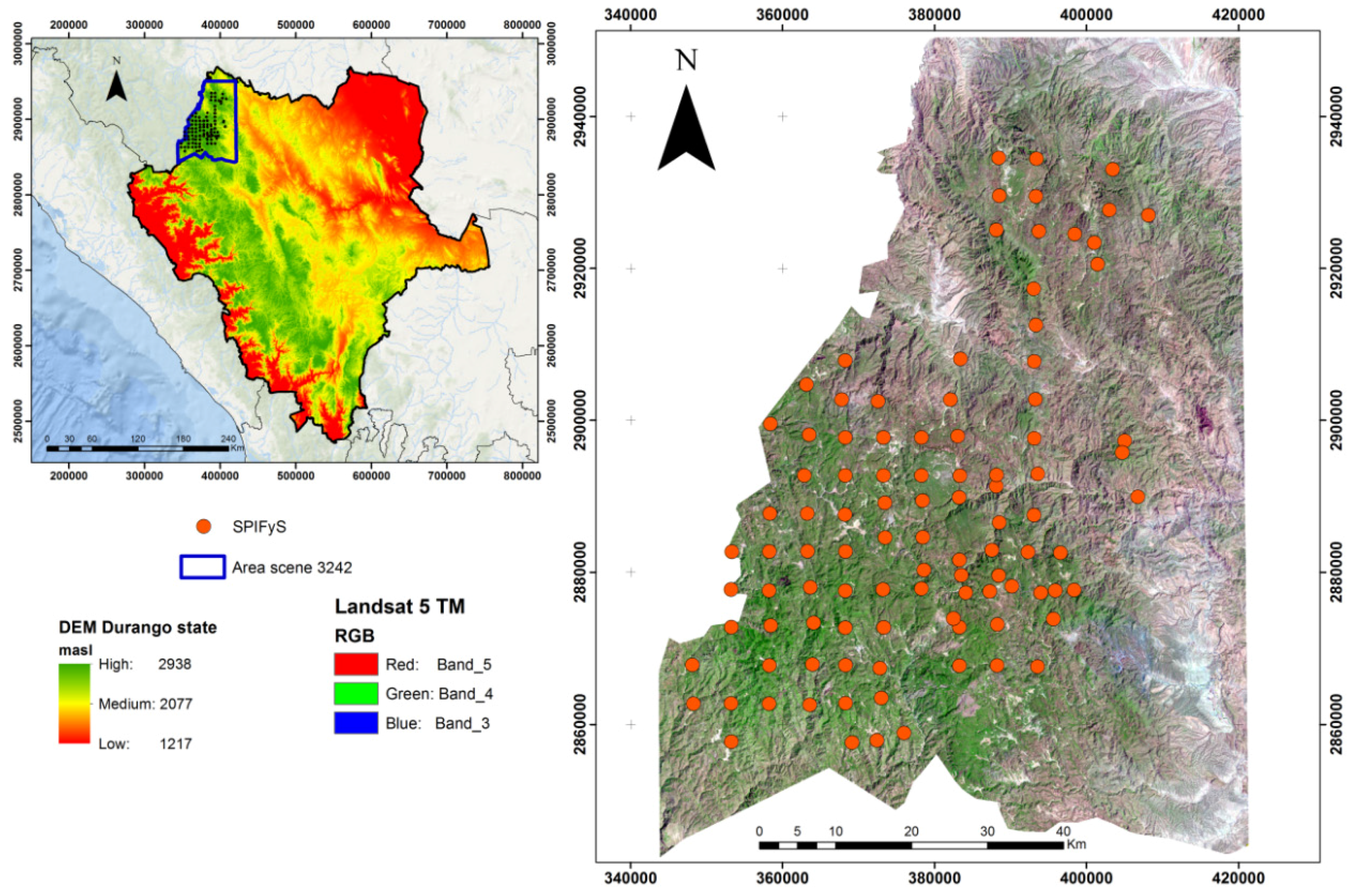
2.1. Study Area
2.2. Field Data
2.3. Spectral Data from the Landsat 5 TM Sensor
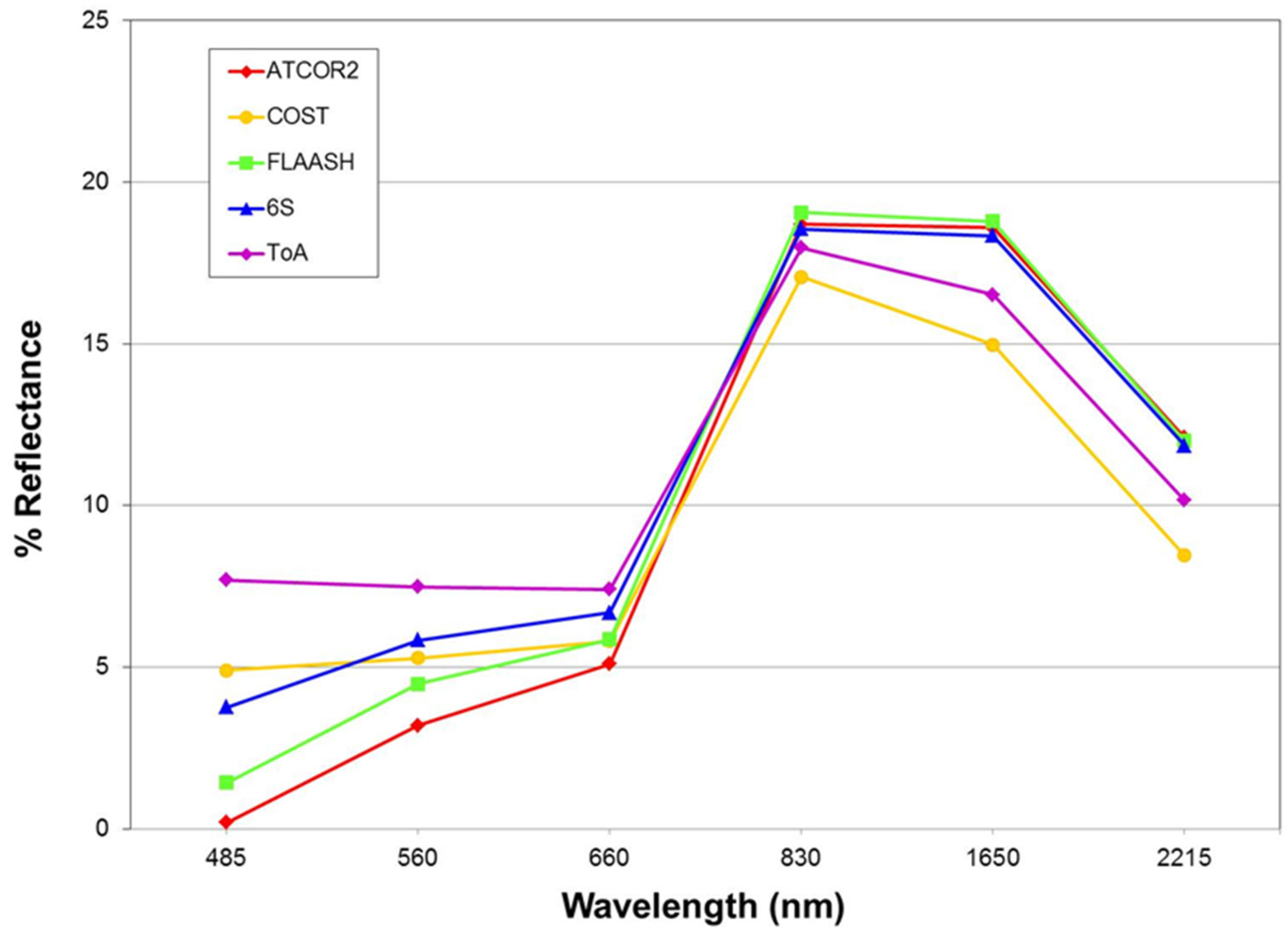
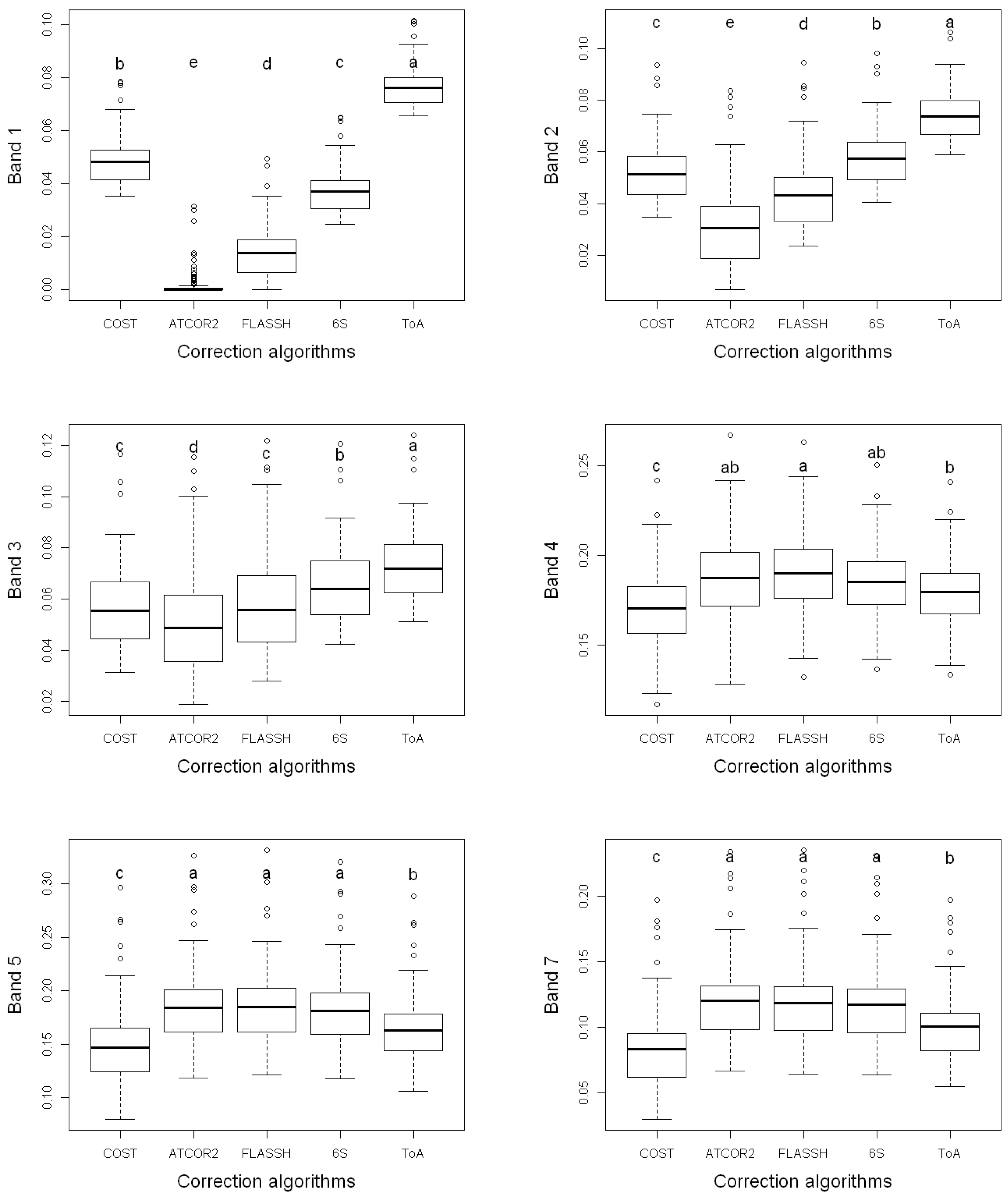
2.4. Radiometric Correction Algorithms
2.4.1. Atmospheric Correction for Flat Terrain (ATCOR2)
2.4.2. Cosine of the Sun Zenith Angle (COST)
2.4.3. Fast Line-of-Sight Atmospheric Analysis of Spectral Hypercubes (FLAASH)
2.4.4. Second Simulation of Satellite Signal in the Solar Spectrum (6S)
2.4.5. Apparent Reflectance at the Top of Atmosphere (ToA)
2.5. Parameters Derived from the Digital Elevation Model (DEM)
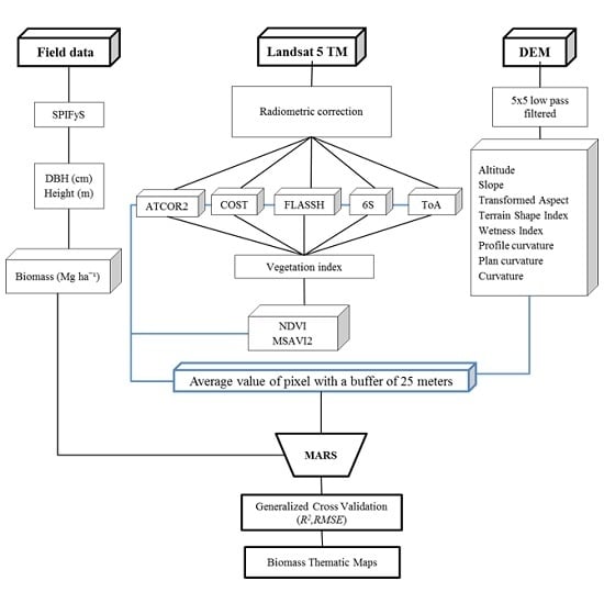
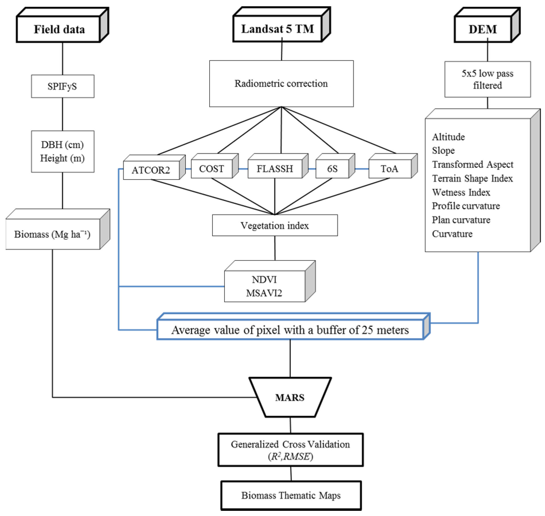
2.6. Generation of a Database
2.7. Statistical Analysis
2.7.1. Analysis of Variance
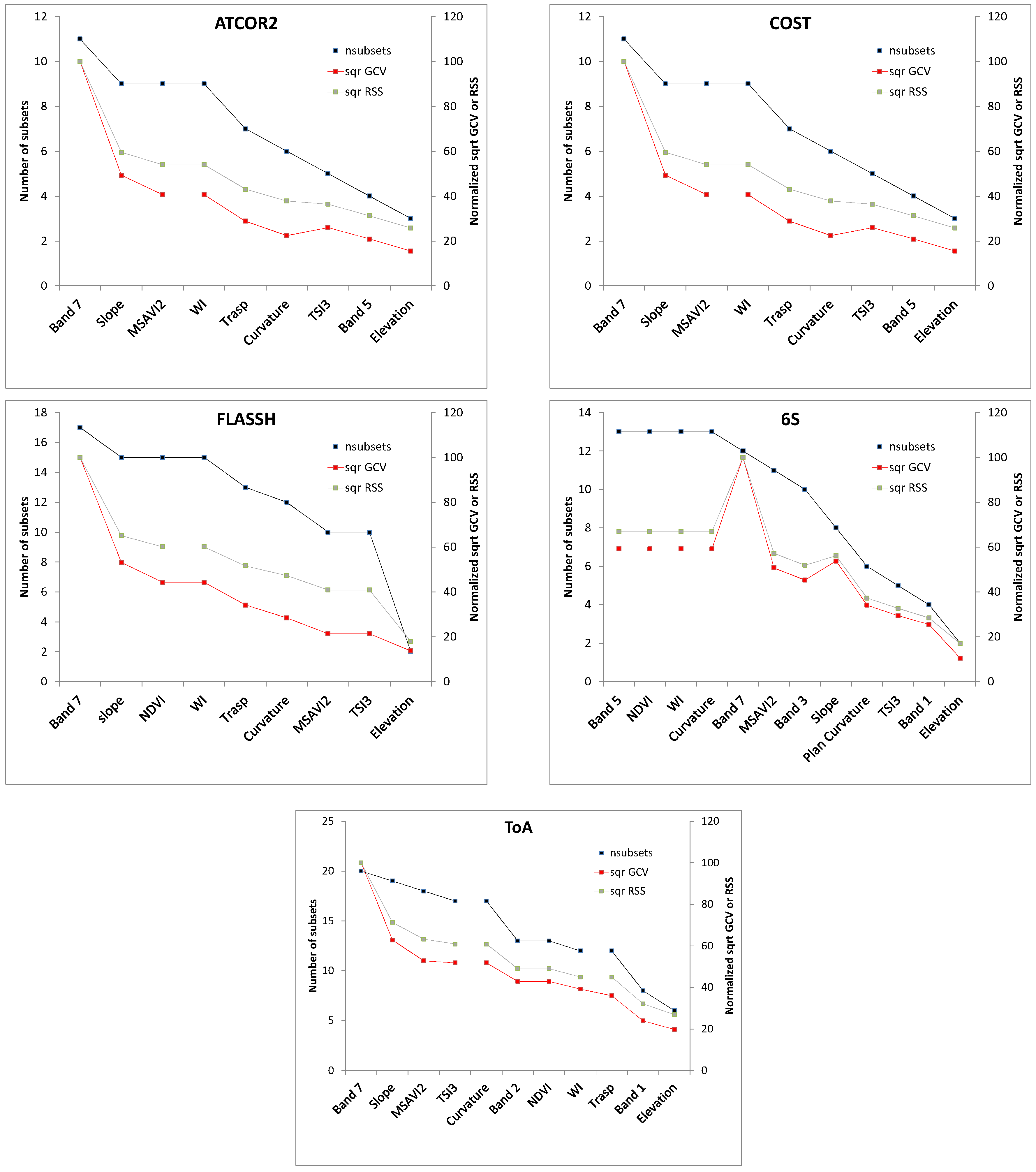
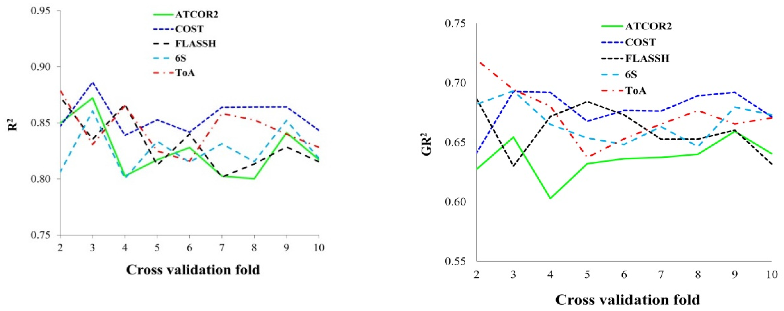
2.7.2. Multivariate Adaptive Regression Spline (MARS)
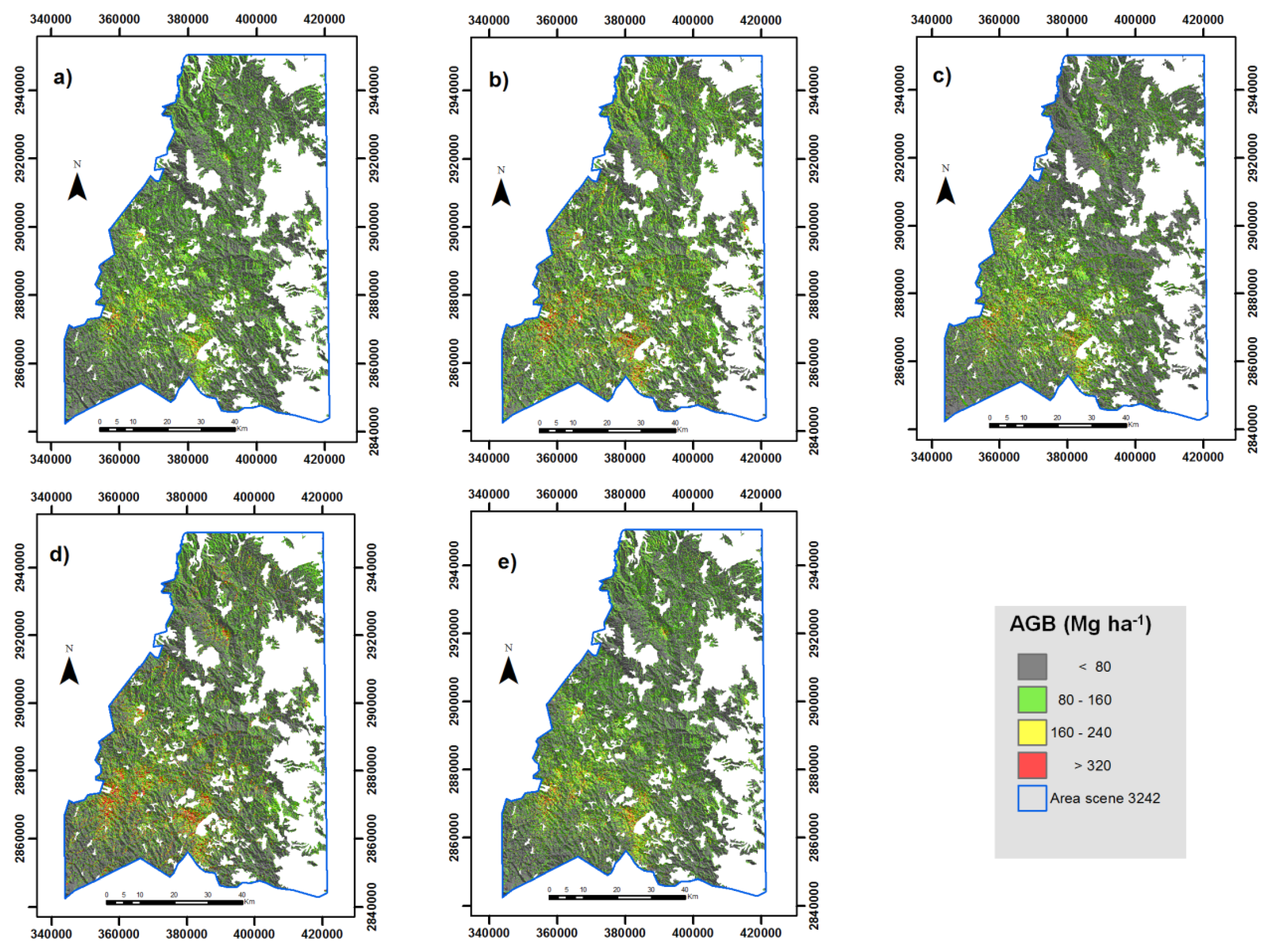
2.8. Generation of Thematic Maps
3. Results
4. Discussion
5. Conclusions
Acknowledgments
Author Contributions
Conflicts of Interest
References
- Jensen, J.R. A remote sensing perspective. In Introductory Digital Image Processing; Prentice Hall: Englewood Cliffs, NJ, USA, 1996. [Google Scholar]
- Gao, B.C.; Montes, M.J.; Davis, C.O.; Goetz, A.F. Atmospheric correction algorithms for hyperspectral remote sensing data of land and ocean. Remote Sens. Environ. 2009, 113, S17–S24. [Google Scholar] [CrossRef]
- Tyagi, P.; Bhosle, U. Atmospheric correction of remotely sensed images in spatial and transform domain. Int. J. Image Process. 2011, 5, 564–579. [Google Scholar]
- Tan, K.C.; Lim, H.S.; Matjafri, M.Z.; Adbullah, K. A comparison of radiometric correction techniques in the evaluation between LST and NDVI in Landsat imagery. Environ. Monit. Assess. 2012, 184, 3813–3829. [Google Scholar] [CrossRef] [PubMed]
- Hadjimitsis, D.G.; Papadavid, G.; Agapiou, A.; Themistocleous, K.; Hadjimitsis, M.G.; Retalis, A.; Michaelides, S.; Chrysoulakis, N.; Toulios, L.; Clayton, C.R.I. Atmospheric correction for satellite remotely sensed data intended for agricultural applications: Impact on vegetation indices. Nat. Hazards Earth Syst. Sci. 2010, 10, 89–95. [Google Scholar] [CrossRef]
- Li, F.; Jupp, D.L.; Thankappan, M.; Lymburner, L.; Mueller, N.; Lewis, A.; Held, A. A physics-based atmospheric and BRDF correction for Landsat data over mountainous terrain. Remote Sens. Environ. 2012, 124, 756–770. [Google Scholar] [CrossRef]
- Jaelani, L.M.; Matsushita, B.; Yang, W.; Fukushima, T. An improved atmospheric correction algorithm for applying MERIS data to very turbid inland waters. Int. J. Appl. Earth Obs. Geoinform. 2015, 39, 128–141. [Google Scholar] [CrossRef]
- Lee, C.S.; Yeom, J.M.; Lee, H.L.; Kim, J.J.; Han, K.S. Sensitivity analysis of 6S-based look-up table for surface reflectance retrieval. Asia Pac. J. Atmos. Sci. 2015, 51, 91–101. [Google Scholar] [CrossRef]
- Vanonckelen, S.; Lhermitte, S.; Van Rompaey, A. The effect of atmospheric and topographic correction methods on land cover classification accuracy. Int. J. Appl. Earth Obs. Geoinform. 2013, 24, 9–21. [Google Scholar] [CrossRef]
- Moreira, E.P.; Valeriano, M.M. Application and evaluation of topographic correction methods to improve land cover mapping using object-based classification. Int. J. Appl. Earth Obs. Geoinform. 2014, 32, 208–217. [Google Scholar] [CrossRef]
- Roy, D.; Wulder, M.; Loveland, T.; Woodcock, C.; Allen, R.; Anderson, M. LANDSAT-8: Science and product vision for terrestrial global change research. Remote Sens. Environ. 2014, 145, 154–172. [Google Scholar] [CrossRef]
- Ju, J.; Roy, D.; Vermote, E.; Masek, J.; Kovalsky, V. Continental-scale validation of MODIS-based and LEDAPS Landsat ETM+ atmospheric correction methods. Remote Sens. Environ. 2012, 122, 175–184. [Google Scholar] [CrossRef]
- Ediriweera, S.; Pathirana, S.; Danaher, T.; Nichols, D.; Moffiet, T. Evaluation of different topographic corrections for Landsat TM data by prediction of foliage projective cover (FPC) in topographically complex landscapes. Remote Sens. 2013, 5, 6767–6789. [Google Scholar] [CrossRef]
- Gagliasso, D.; Hummel, S.; Temesgen, H. A comparison of selected parametric and non-parametric imputation methods for estimating forest biomass and basal area. Open J. For. 2014, 4, 42–48. [Google Scholar] [CrossRef]
- Hantson, S.; Chuvieco, E. Evaluation of different topographic correction methods for Landsat imagery. Int. J. Appl. Earth Obs. Geoinform. 2011, 13, 691–700. [Google Scholar] [CrossRef]
- Balthazar, V.; Veerle, V.; Eric, F.L. Evaluation and parameterization of ATCOR3 topographic correction method for forest cover mapping in mountain areas. Int. J. Appl. Earth Obs. Geoinform. 2012, 18, 436–450. [Google Scholar] [CrossRef]
- Cortés, L.; Hernández, J.; Valencia, D.; Corvalán, P. Estimation of above-ground forest biomass using Landsat ETM+, Aster GDEM and Lidar. Forest Res. 2014. [Google Scholar] [CrossRef]
- Kelsey, K.C.; Neff, J.C. Estimates of aboveground biomass from texture analysis of landsat imagery. Remote Sens. 2014, 6, 6407–6422. [Google Scholar] [CrossRef]
- Tian, X.; Li, Z.; Su, Z.; Chen, E.; Van der Tol, C.; Li, X.; Guo, Y.; Li, L.; Ling, F. Estimating montane forest above-ground biomass in the upper reaches of the Heihe River Basin using Landsat-TM data. Int. J. Remote Sens. 2014, 35, 7339–7362. [Google Scholar] [CrossRef]
- Vincent, R.K. An ERTS multispectral scanner experiment for mapping iron compounds. In Proceedings of the 8th International Symposium on Remote Sensing of Environment, Ann Arbor, MI, USA, 2–6 October 1972; pp. 1239–1247.
- Chavez, P.S. Image-based atmospheric corrections-revisited and improved. Photogramm. Eng. Remote Sens. 1996, 62, 1025–1036. [Google Scholar]
- Richter, R. A spatially adaptive fast atmospheric correction algorithm. Int. J. Remote Sens. 1996, 17, 1201–1214. [Google Scholar] [CrossRef]
- Adler-Golden, S.; Berk, A.; Bernstein, L.S.; Richtsmeier, S.; Acharya, P.K.; Matthew, M.W.; Anderson, G.P.; Allred, C.L.; Jeong, L.S.; Chetwynd, J.H. FLAASH, a MODTRAN4 atmospheric correction package for hyperspectral data retrievals and simulations. In Procedings of the 7th Annual JPL Airborne Earth Science Workshop, Pasadena, CA, USA, 12–16 January 1998; Green, R.O., Ed.; pp. 9–14.
- Anderson, G.P.; Felde, G.W.; Hoke, M.L.; Ratkowski, A.J.; Cooley, T.W.; Chetwynd, J.H., Jr.; Gardner, J.A.; Adler-Golden, S.M.; Matthew, M.W.; Berk, A.; et al. MODTRAN4-based atmospheric correction algorithm: FLAASH (fast line-of-sight atmospheric analysis of spectral hypercubes). In Algorithms and Technologies for Multispectral, Hyperspectral, and Ultraspectral Imagery VIII (Proceedings of SPIE); Shen, S.S., Lewis, P.E., Eds.; Society of Photo Optics: Orlando, FL, USA, 2002; pp. 65–71. [Google Scholar]
- Vermote, E.F.; Tanre, D.; Deuze, J.L.; Herman, M.; Morcette, J.J. Second simulation of the satellite signal in the solar spectrum, 6S: An overview. IEEE Trans. Geosci. Remote 1997, 35, 675–686. [Google Scholar] [CrossRef]
- Saatchi, S.S.; Harris, N.L.; Brown, S.; Lefsky, M.; Mitchard, E.T.A.; Salas, W.; Zutta, B.R.; Buermann, W.; Lewis, S.L.; Hagen, S.; et al. Benchmark map of forest carbon stocks in tropical regions across three continents. Proc. Natl. Acad. Sci. USA 2011, 108, 9899–9904. [Google Scholar] [CrossRef] [PubMed]
- Moisen, G.G.; Frescino, T.S. Comparing five modelling techniques for predict-ing forest characteristics. Ecol. Model. 2002, 157, 209–225. [Google Scholar] [CrossRef]
- Güneralp, I.; Filippi, A.M.; Randall, J. Estimation of floodplain aboveground biomass using multispectralremote sensing and nonparametric modeling. Int. J. Appl. Earth Obs. Geoinform. 2014, 33, 119–126. [Google Scholar] [CrossRef]
- Filippi, A.M.; Güneralp, I.; Randall, J. Hyperspectral remote sensing of above-ground biomass on a river meander bend using multivariate adaptive regressionsplines and stochastic gradient boosting. Remote Sens. Lett. 2014, 5, 432–441. [Google Scholar] [CrossRef]
- Instituto Nacional de Estadística Geográfica e Informática (INEGI). Uso del Suelo y Vegetación Escala 1:250 000 Serie V, Información Vectorial; Instituto Nacional de Estadística Geográfica e Informática: Ciudad de Mexico, Mexico, 2012. [Google Scholar]
- Corral-Rivas, J.J.; Vargas, B.; Wehenkel, C.; Aguirre, O.; Álvarez, J.G.; Rojo, A. Guía para el Establecimiento de Sitios de Inventario Periódico Forestal y de Suelos del Estado de Durango; Facultad de Ciencias Forestales: Universidad Juárez del Estado de Durango, Durango, México, 2009. [Google Scholar]
- Vargas-Larreta, B. Estimación del Potencial de los Bosques de Durango Para la Mitigación del Cambio Climático. Modelización de la Biomasa Forestal. Proyecto FOMIX-DGO-2011-C01-165681; Comisión Nacional de Ciencia y Tecnología (CONACYT): Durango, Mexico, 2013. [Google Scholar]
- United States Geological Survey. Available online: http://glovis.usgs.gov (accessed on 11 January 2011).
- Rouse, J.W.; Haas, R.H.; Schell, J.A.; Deering, D.W.; Harlan, J.C. Monitoring the Vernal Advancements and Retrogradation (Greeen Wave Effect) of Natural Vegetation; NASA/GFSC: Greenbelt, MD, USA, 1974. [Google Scholar]
- Baret, F.; Guyot, G. Potentials and limits of vegetation indices for LAI and APAR assessment. Remote Sens. Environ. 1991, 35, 161–173. [Google Scholar] [CrossRef]
- Lavreau, J. De-hazing landsat thematic mapper images. Photogramm. Eng. Remote Ssens. 1991, 57, 1297–1302. [Google Scholar]
- Guyot, G.; Gu, X.F. Effect of radiometric corrections on NDVI-determined from SPOT-HRV and Landsat-TM data. Remote Sens. Environ. 1994, 49, 169–180. [Google Scholar] [CrossRef]
- Richter, R. Atmospheric correction of satellite data with haze removal including a haze/clear transition region. Comput. Geosci. 1996, 22, 675–681. [Google Scholar] [CrossRef]
- Carlotto, M.J. Reducing the effects of space-varying, wavelength-dependent scattering in multispectral imagery. Int. J. Remote Sens. 1999, 20, 3333–3344. [Google Scholar] [CrossRef]
- Song, C.; Woodcock, C.E.; Seto, K.C.; Lenney, M.P.; Macomber, S.A. Classification and change detection using Landsat TM data: When and how to correct atmospheric effects? Remote Sens. Environ. 2001, 75, 230–244. [Google Scholar] [CrossRef]
- Liang, S.; Fang, H.; Morisette, J.T.; Chen, M.; Shuey, C.J.; Walthall, C.L.; Daughtry, C.S.T. Atmospheric correction of Landsat ETM+ land surface imagery. II. Validation and applications. IEEE Trans. Geosci. Remote Sens. 2002, 40, 2736–2746. [Google Scholar] [CrossRef]
- Chuvieco, E. Teledetección Ambiental: La Observación de la Tierra, 1st ed.; Ariel Ciencia: Madrid, Spain, 2010. [Google Scholar]
- Geosystems. Haze Reduction, Atmospheric and Topographic Correction. User Manual ATCOR2 and ATCOR3; Geosystems GmbH: Geneva, Switzerland, 2013. [Google Scholar]
- ERDAS Inc. Erdas Imagine. Available online: http://www.hexagongeospatial.com/products/ERDAS-IMAGINE/details.aspx (accessed on 6 October 2014).
- Chavez, P.S. An improved dark-object subtraction technique for atmospheric scattering correction of multispectral data. Remote Sens. Environ. 1988, 24, 459–479. [Google Scholar] [CrossRef]
- Moran, M.S.; Jackson, R.D.; Slater, P.N.; Teillet, P.M. Evaluation of simplified procedures for retrieval of land surface reflectance factors from satellite sensor output. Remote Sens. Environ. 1992, 41, 169–184. [Google Scholar] [CrossRef]
- EXELIS Inc. ENVI® 5.1 Fast Line-of-Sight Atmospheric Analysis of Hypercubes (FLAASH); EXELIS Inc.: Boulder, CO, USA, 2013. [Google Scholar]
- Huang, C.; Yang, L.; Homer, C.; Wylie, B.; Vogelman, J.; DeFelice, T. At Satellite Reflectance: A First Order Normalization of LANDSAT 7 ETM+ Images. Available online: http://digitalcommons.unl.edu/usgspubs/109/ (accessed on 6 October 2014).
- Goslee, S. Radiometric and Topographic Correction of Satellite Imagery. Package Landsat. Version 1.0.8. Available online: http://cran.r-project.org/web/packages/landsat/landsat.pdf (accessed on 18 May 2015).
- R Core Team. R: A Language and Environment for Statistical Computing, R Foundation for Statistical Computing. Available online: http://www.R-project.org/ (accessed on 18 March 2014).
- Instituto Nacional de Estadística Geográfica e Informática (INEGI). México Continuo de Elevaciones Mexicano 3.0 (CEM 3.0). Available online: http://www.inegi.org.mx/geo/contenidos/datosrelieve/continental/descarga.aspx (accessed on 6 May 2014).
- McNab, W.H. Terrain shape index: quantifying effect of minor landforms on tree height. Forest Sci. 1989, 35, 91–104. [Google Scholar]
- Roberts, D.W.; Cooper, S.V. Concepts and techniques of vegetation mapping. In Land Classifications Based on Vegetation: Applications for Resource Management; Ferguson, D., Morgan, P., Johnson, F.D., Eds.; General technical report INT-US Department of Agriculture, Forest Service, Intermountain Research Station (USA): Ogden, UT, USA, 1989; pp. 90–96. [Google Scholar]
- Moore, I.D.; Nieber, J.L. Landscape assessment of soil erosion and non-point source pollution. J. Minn. Acad. Sci. 1989, 55, 18–24. [Google Scholar]
- Wilson, J.P.; Gallant, J.C. Digital terrain analysis. In Terrain Analysis: Principles and Applications; Wilson, J.P., Gallant, J.C., Eds.; John Wiley & Sons, Inc.: New York, NY, USA, 2000; pp. 1–28. [Google Scholar]
- Zevenbergen, L.W.; Thorne, C.R. Quantitative analysis of land surface topography. Earth Surf. Proc. Landf. 1987, 12, 47–56. [Google Scholar] [CrossRef]
- Hijmans, R.J. Raster: Geographic Data Analysis and Modeling. R Package Version 2.4-20. Available online: http://CRAN.R-project.org/package=raster (accessed on 6 October 2015).
- Shapiro, S.S.; Wilk, M.B. An analysis of variance test for normality (complete samples). Biometrika 1965, 52, 591–611. [Google Scholar] [CrossRef]
- Levene, H. Robust tests for equality of variances. In Contributions to Probability and Statistics: Essays in Honor of Harold Hotelling; Olkin, I., Ed.; Stanford University Press: Stanford, CA, USA, 1960; pp. 278–292. [Google Scholar]
- Friedman, J.H. Multivariate adaptive regression spline. Ann. Stat. 1991, 19, 1–141. [Google Scholar] [CrossRef]
- Milborrow, S. Earth: Multivariate Adaptive Regression Splines. R Package Version 4.2.0. Available online: http://CRAN.R-project.org/package=earth (accessed on 6 October 2015).
- Myers, R.H. Classical and Modern Regression with Applications; PWS-Kent Publishing Company: Belmont, CA, USA, 1990. [Google Scholar]
- ESRI Inc. ArcGIS Desktop: Release 10; Environmental Systems Research Institute: Redlands, CA, USA, 2011. [Google Scholar]
- Fernández, S.C.; Rodenas, A.Q. Teledetección: Avances y Aplicaciones; Diputación de Albacete: Albacete, Spain, 1999. [Google Scholar]
- Buho, H.; Kaneko, M.; Ogawa, K. Correction of NDVI calculated from ASTER L1B and ASTER (AST07) data based on ground measurement. In Advances in Geoscience and Remote Sensing; Jedlovec, G., Ed.; In-Tech Press: Vienna, Austria, 2009. [Google Scholar]
- Richter, R.; Schläpfer, D. Atmospheric/Topographic Correction for Satellite Imagery. ATCOR 2/3 User Guide, Version 9.0.0.; ReSe Applications Schläpfer: Langeggweg, Switzerland, 2015. [Google Scholar]
- Broszeit, A.; Ashraf, S. Using different atmospheric correction methods to classify remotely sensed data to detect liquefaction of the February 2011 earthquake in Christchurch. In Proceedings of the SIRC NZ 2013—GIS and Remote Sensing Research Conference, Dunedin, New Zealand, 29–30 August 2013.
- Nazeer, M.; Nichol, J.E.; Yung, Y.K. Evaluation of atmospheric correction models and Landsat surface reflectance product in an urban coastal environment. Int. J. Remote Sens. 2014, 35, 6271–6291. [Google Scholar] [CrossRef]
- Mahiny, A.S.; Turner, B.J. A comparison of four common atmospheric correction methods. Photogramm. Eng. Remote Sens. 2007, 73, 361–368. [Google Scholar] [CrossRef]
- Hamdan, O.; Hasmadi, I.M.; Aziz, H.K. Combination of SPOT-5 and ALOS PALSAR images in estimating aboveground biomass of lowland Dipterocarp forest. In Proceedings of the IOP Conference Series: Earth and Environmental Science, Tomst, Russia, 7–11 April 2014.
- Nguyen, H.C.; Jung, J.; Lee, J.; Choi, S.U.; Hong, S.Y.; Heo, J. Optimal atmospheric correction for above-ground forest biomass estimation with the ETM+ remote sensor. Sensors 2015, 15, 18865–18886. [Google Scholar] [CrossRef] [PubMed]
- Bilgili, A.V.; Van Es, H.M.; Akbas, F.; Durak, A.; Hively, W.D. Visible-near infrared, reflectance spectroscopy for assessment of soil properties in a semi-arid area of Turkey. J. Arid Environ. 2010, 74, 229–238. [Google Scholar] [CrossRef]
- Ghasemi, J.B.; Zolfonoun, E. Application of principal component analysis-multivariate adaptive regression splines for the simultaneous spectrofluorimetric determination of dialkyltins in micellar media. Spectrochim. Spectrochimi. Acta Part A Mol. Biomol. Spectrosc. 2013, 115, 357–363. [Google Scholar] [CrossRef] [PubMed]
- García, M.A.; Pérez, C.F.; De la Riva, J.; Fernández, J.; Pascual, P.E.; Herranz, A. Estimación de la biomasa residual forestal mediante técnicas de teledetección y SIG en masas puras de Pinus halepensis y P. sylvestris. In Proceedings of the IV Congreso Forestal Español, Zaragoza, Spain, 26–30 September 2005.
- López-Serrano, P.M.; López-Sánchez, C.A.; Díaz-Varela, R.A.; Corral-Rivas, J.J.; Solís-Moreno, R.; Vargas-Larreta, B.; Álvarez-González, J.G. Estimating biomass of mixed and uneven-aged forests using spectral data and a hybrid model combining regression trees and linear models. iForest 2015. [Google Scholar] [CrossRef]
- Lam, C.S.Y. Comparison of Flow Routing Algorithms Used in Geographic Information Systems. Ph.D. Thesis, University of Southern California, Los Angeles, CA, USA, 2004. [Google Scholar]
- Hoechstetter, S.; Walz, U.; Dang, L.H.; Thinh, N.X. Effects of topography and surface roughness in analyses of landscape structure–A proposal to modify the existing set of landscape metrics. Landsc. Online 2008, 3, 1–14. [Google Scholar] [CrossRef]
- Sesnie, S.E.; Dickson, B.D.; Rosenstock, S.S.; Rundall, J.M. A comparison of Landsat TM and MODIS vegetation indices for estimating forage phenology in desert bighorn sheep (Ovis canadensis nelsoni) habitat in the Sonoran Desert, USA. Int. J. Remote Sens. 2012, 33, 276–286. [Google Scholar] [CrossRef]
- Ali, M.; Montzka, C.; Stadler, A.; Menz, G.; Thonfeld, F.; Vereecken, H. Estimation and validation of rapideye-based time-series of leaf area index for winter wheat in the rur catchment (Germany). Remote Sens. 2015, 7, 2808–2831. [Google Scholar] [CrossRef]
- Yao, Z.; Liu, J.; Zhao, X.; Long, D.; Wang, L. Spatial dynamics of aboveground carbon stock in urban green space: A case study of Xi’an, China. J. Arid Land. 2015, 7, 350–360. [Google Scholar] [CrossRef]


| Variable | Mean | Standard Deviation | Minimum Value | Maximum Value |
|---|---|---|---|---|
| Number of stems per ha | 655.47 | 322.25 | 224 | 2264 |
| Diameter at breast height (cm) | 18.44 | 3.46 | 11.69 | 31.12 |
| Dominant height (m) | 14.62 | 3.72 | 6.87 | 24.81 |
| Stand biomass (Mg·ha−1) | 89.03 | 43.45 | 2.70 | 234.03 |
| Variable | Formula | Reference |
|---|---|---|
| Elevation | Digital Elevation Model | |
| Slope (β) | β = arctan | |
| Transformed aspect (Trasp) | Trasp = | [53] |
| Terrain Shape Index (TSI) | TSI = /R | [52] |
| Wetness Index (WI) | WI = ln (As/tanβ) | [54] |
| Profile curvature (Ø) | [55] | |
| Plan curvature (ω) | ||
| Curvature (x) | x = − |
| Algorithm | Number of Terms | Number of Predictors | GCV | RSS | GR2 | R2 | RMSE | %RMSE |
|---|---|---|---|---|---|---|---|---|
| ATCOR2 | 12 of 31 | 9 of 17 | 780.84 | 45556.61 | 0.59 | 0.75 | 50.37 | 56.58 |
| COST | 16 of 29 | 9 of 17 | 572.13 | 26722.49 | 0.70 | 0.85 | 36.55 | 41.05 |
| FLAASH | 18 of 33 | 9 of 17 | 737.91 | 30530.20 | 0.61 | 0.83 | 36.43 | 40.92 |
| 6S | 16 of 30 | 12 of 17 | 552.26 | 25794.27 | 0.71 | 0.86 | 33.48 | 37.61 |
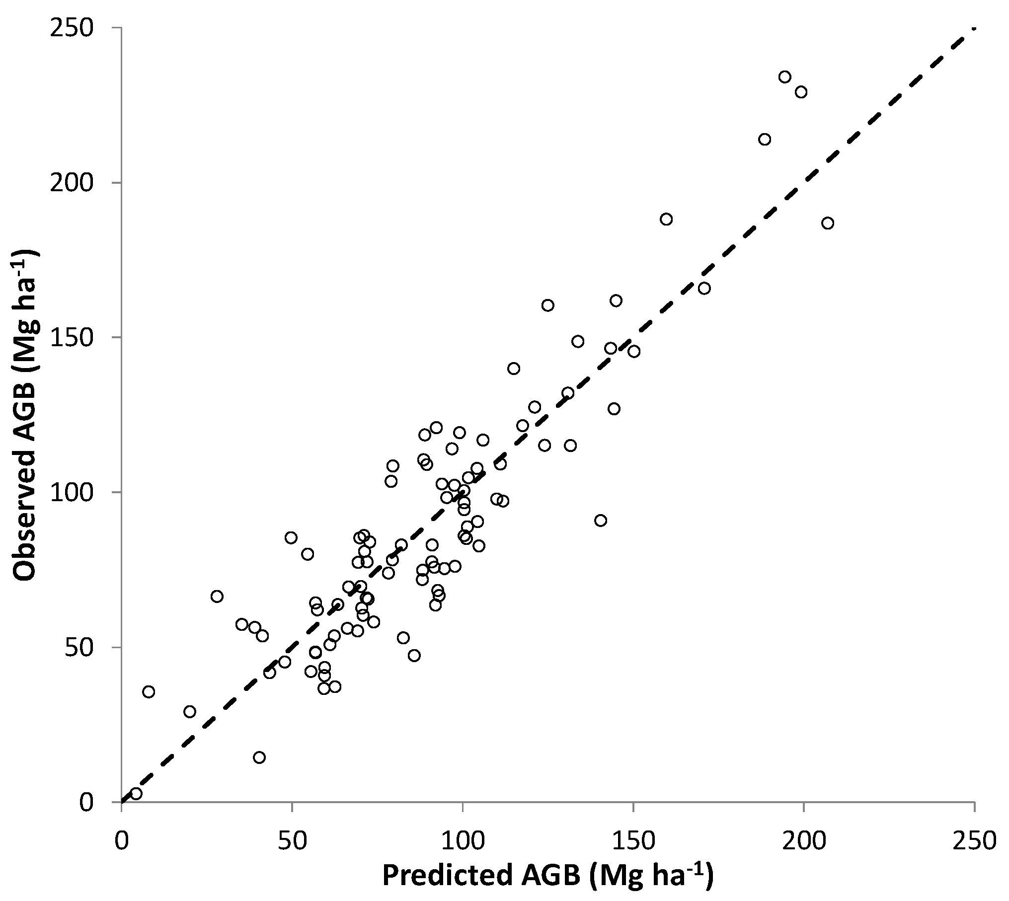
| ToA | 21 of 30 | 11 of 17 | 601.91 | 20452.83 | 0.68 | 0.89 | 29.82 | 33.49 |
© 2016 by the authors; licensee MDPI, Basel, Switzerland. This article is an open access article distributed under the terms and conditions of the Creative Commons Attribution (CC-BY) license (http://creativecommons.org/licenses/by/4.0/).
Share and Cite
López-Serrano, P.M.; Corral-Rivas, J.J.; Díaz-Varela, R.A.; Álvarez-González, J.G.; López-Sánchez, C.A. Evaluation of Radiometric and Atmospheric Correction Algorithms for Aboveground Forest Biomass Estimation Using Landsat 5 TM Data. Remote Sens. 2016, 8, 369. https://doi.org/10.3390/rs8050369
López-Serrano PM, Corral-Rivas JJ, Díaz-Varela RA, Álvarez-González JG, López-Sánchez CA. Evaluation of Radiometric and Atmospheric Correction Algorithms for Aboveground Forest Biomass Estimation Using Landsat 5 TM Data. Remote Sensing. 2016; 8(5):369. https://doi.org/10.3390/rs8050369
Chicago/Turabian StyleLópez-Serrano, Pablito M., José J. Corral-Rivas, Ramón A. Díaz-Varela, Juan G. Álvarez-González, and Carlos A. López-Sánchez. 2016. "Evaluation of Radiometric and Atmospheric Correction Algorithms for Aboveground Forest Biomass Estimation Using Landsat 5 TM Data" Remote Sensing 8, no. 5: 369. https://doi.org/10.3390/rs8050369