Article

Texture Retrieval from VHR Optical Remote Sensed Images Using the Local Extrema Descriptor with Application to Vineyard Parcel Detection

1
Institut Telecom, Telecom Bretagne, CNRS UMR 6285 Lab-STICC/CID, 29238 Brest Cedex 3, France
2
I-Sea (SAS), 33702 Mérignac Cedex, France
3
The French Space Agency (CNES), DCT/SI/AP-BPI 1219, 31401 Toulouse Cedex 09, France
*
Authors to whom correspondence should be addressed.
Remote Sens. 2016, 8(5), 368; https://doi.org/10.3390/rs8050368
Submission received: 15 February 2016 / Revised: 31 March 2016 / Accepted: 25 April 2016 / Published: 28 April 2016

Abstract

:
In this article, we develop a novel method for the detection of vineyard parcels in agricultural landscapes based on very high resolution (VHR) optical remote sensing images. Our objective is to perform texture-based image retrieval and supervised classification algorithms. To do that, the local textural and structural features inside each image are taken into account to measure its similarity to other images. In fact, VHR images usually involve a variety of local textures and structures that may verify a weak stationarity hypothesis. Hence, an approach only based on characteristic points, not on all pixels of the image, is supposed to be relevant. This work proposes to construct the local extrema-based descriptor (LED) by using the local maximum and local minimum pixels extracted from the image. The LED descriptor is formed based on the radiometric, geometric and gradient features from these local extrema. We first exploit the proposed LED descriptor for the retrieval task to evaluate its performance on texture discrimination. Then, it is embedded into a supervised classification framework to detect vine parcels using VHR satellite images. Experiments performed on VHR panchromatic PLEIADES image data prove the effectiveness of the proposed strategy. Compared to state-of-the-art methods, an enhancement of about 7% in retrieval rate is achieved. For the detection task, about 90% of vineyards are correctly detected.

Graphical Abstract

1. Introduction

Exploiting satellite image data to understand and monitor the land cover and land use from the Earth’s surface in general, particularly in agriculture, is one of the most significant tasks of remote sensing. In this work, we carry out a study of vineyard cultivation by detecting vine parcels using VHR optical remotely-sensed images. In particular, our motivation is to perform a supervised classification algorithm to distinguish vineyard parcels from other items present from the image content, such as forest zones, bare soils, early grown grasses, urban areas, etc. In order to to that, we first propose a novel descriptor to characterize structural and textural features from the image. A retrieval process is then proposed to validate and confirm the performance of this novel descriptor. Then, a supervised classification process is carried out to detect vine fields among other classes.
Many research studies have been so far carried out to tackle retrieval and classification tasks in the scope of remote sensing imagery, particularly in vineyard cultivation. Classical statistical texture analysis techniques, such as the gray-level co-occurrence matrix (GLCM) [1], the Gabor filter banks (GFB) [2], the Weber local descriptor (WLD) [3] or the multiscale discrete wavelet decomposition [4], have been investigated and adapted to VHR image data. In [5], GLCM features were exploited for classification of orchards and vineyards using VHR panchromatic images. In [6], they were used to retrieve different forest structure variables from IKONOS-2 images. Next, methods based on the Gabor filter coefficients were proposed in [7,8] for vine plot detection using optical images. In [9,10], multi-resolution texture analysis using wavelet techniques was investigated on VHR remote sensing data. The WLD is not frequently used in the optical remote sensing field, but efforts have been done to study its behavior on VHR polarimetric radar data for patch indexing [11]. Among these approaches, wavelet-based techniques appear to be the most commonly used up to now. Some recent studies have focused on the modeling of wavelet coefficients using multivariate distribution models. In [12,13], the authors studied the multivariate Gaussian models (MGM), the spherically-invariant random vectors (SIRV) and the Gaussian copula-based models (GCM) to tackle texture retrieval and classification of VHR maritime pine forest images.
However, all of the above classical approaches are limited to the use of large dense neighborhoods, which consider all pixels from the image. Hence, they implicitly require the stationarity hypothesis. This condition may not be verified within VHR remote sensing images, where textures appear to be quite heterogeneous with more local features and structures captured from the observed scene. Therefore, their performance on VHR images may be limited. From this point, a non-dense approach based on characteristic points only, not on the whole image’s pixels, could be more relevant. Such an approach does not require any stationary condition. Moreover, it can deal with large-sized VHR image data since only the information and interaction of characteristic points are taken into consideration.
Recently, a pointwise approach based on characteristic pixels has been proposed to tackle the texture characterization task [14,15,16,17]. In these studies, the characteristic points are the local maximum and the local minimum pixels. They are adopted thanks to their capacity to cover all texture zones inside the image. Within such a pointwise approach, only the information and inter-connection of keypoints are considered. Hence, it is capable of dealing with local textures when the stationary hypothesis is weakly verified. In [14,15,16], a weighted graph is constructed to connect those feature points. Then, spectral characteristics from this graph are extracted for texture description. In [17], the authors propose to construct the covariance matrix descriptors based on the local maximum and minimum pixels and prove their efficiency within VHR optical imagery. In this work, we continue and improve the idea of using the local extrema (i.e., local maximum and local minimum pixels) to encode local features from the image. By combining the radiometric, spatial and structural gradient features from these points, the novel local extrema-based descriptor (LED) is proposed. This descriptor is capable of characterizing different types of textures occurring from the image. In particular, it is relevant for retrieving and detecting oriented and structured textures coming from vine fields. We first embed the proposed descriptor into a retrieval framework to validate its capacity of texture description and discrimination. Then, it is exploited to tackle the supervised classification task from which the main motivation is to detect vine parcels. Experimental results show the effectiveness of the proposed retrieval algorithm, particularly in retrieving structural features, such as man-made items in urban zones and different types of aligned vine rows. Then, in terms of vine detection performance, the proposed strategy also provides very promising and competitive results compared to reference methods.
The remainder of the paper is organized as follows. Section 2 describes the studied sites and the VHR image data used in this work. The proposed methodology for the retrieval task with dedicated experiments is detailed in Section 3. Section 4 provides the application of vineyard detection using the proposed descriptor. Finally, a conclusion and some perspective work are discussed in Section 5.

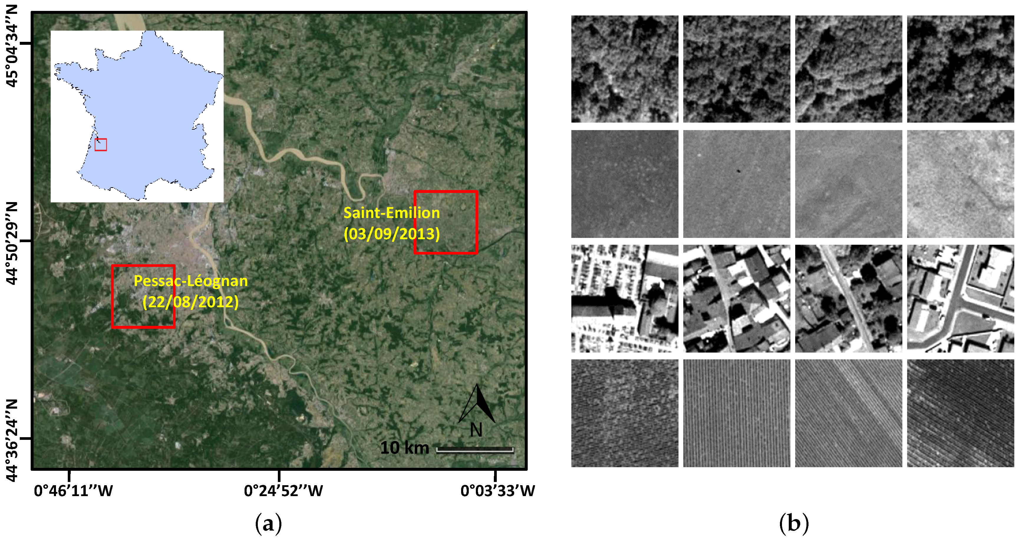
2. Studied Sites and Data

For the study of vine cultivation in this work, we exploit two VHR panchromatic images acquired by the PLEIADES satellite, CNES©, with a spatial resolution of 70 cm at nadir, resampled at 50 cm. These image data were captured from the regions of Pessac-Léognan and Saint-Emilion, both in France (cf. their locations from Figure 1a) on 22 August 2012 and 3 September 2013, respectively. In wine-growing region of Bordeaux, the landscape is mainly dominated by vineyards surrounded by typical peri-urban land covers. A mix of urban, vineyard and forest zones is found from the content of these images. Due to the appearance of different types of textures, four main classes are considered, including the forest, bare soil, urban zones and vine fields. It is worth noting that within the vineyard class, there are several vine parcels that are planted under different orientations, as well as from different development stages. For the retrieval process, a texture database, with a non-equivalent number of 128 × 128 pixel image patches per class, was created from each of the two images. We note that there exist some confusions among classes, especially between the bare soil and vine classes. There are several damaged or dead vine fields, which destroy the aligned structures of vine textures. In addition, vine fields with the row spacing close to the satellite resolution may introduce smooth and mitigated textures, which become similar to bare soils. Related to this point, in the Saint-Emilion region, vine row spacing varies from 1.4 m to 2 m. Hence, the aligned row structures appear quite clearly within vine fields. On the other hand, the Pessac-Léognan region involves vine parcels with row spacing close to 1 m. The vine textures are thus mitigated and become more homogeneous. Therefore, although there are only four classes from each database, it is still challenging for the texture retrieval task.
For a better explanation, the two databases are named Pessac 22-08-12 (including 445 patches in total) and Emilion 03-09-13 (including 984 patches) in the rest of the paper. Figure 1b illustrates some texture patches of the four classes from the Emilion 03-09-13 database. In Section 4, each of the databases will be exploited as the training set for supervised classification. The main purpose is to detect vine parcels from each of the two acquired images.

3. Texture Retrieval from VHR Optical Remote Sensing Images

The proposed texture retrieval algorithm consists of two primary stages: the extraction of the local extrema descriptor (LED) to characterize textural features of each query image from the texture database and the computation of the distance measure for retrieval process. We now address each of them in detail before providing some experimental results compared to other retrieval methods. Furthermore, a study of the algorithm sensitivity to its parameters is carried out in Section 3.5.

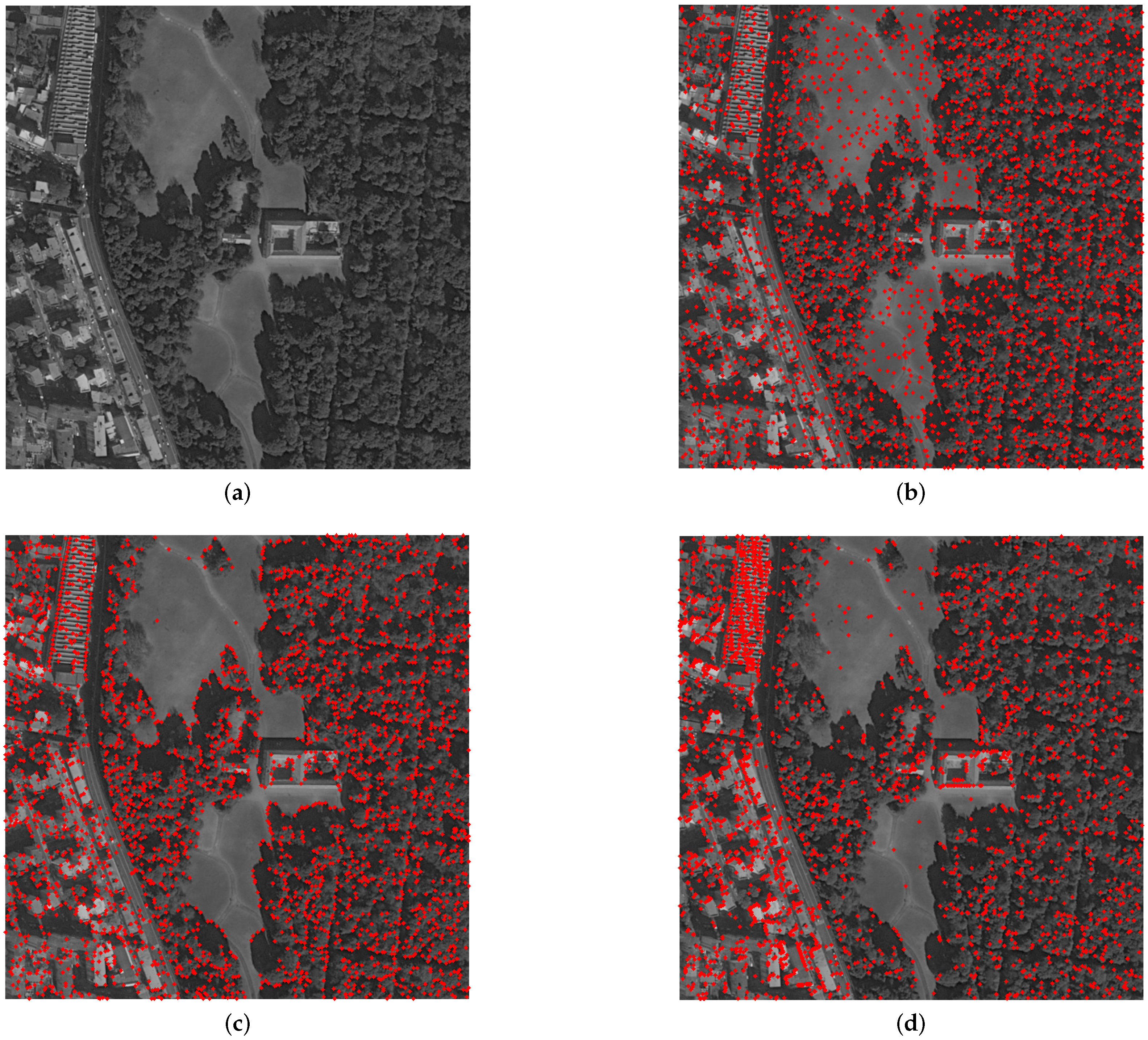
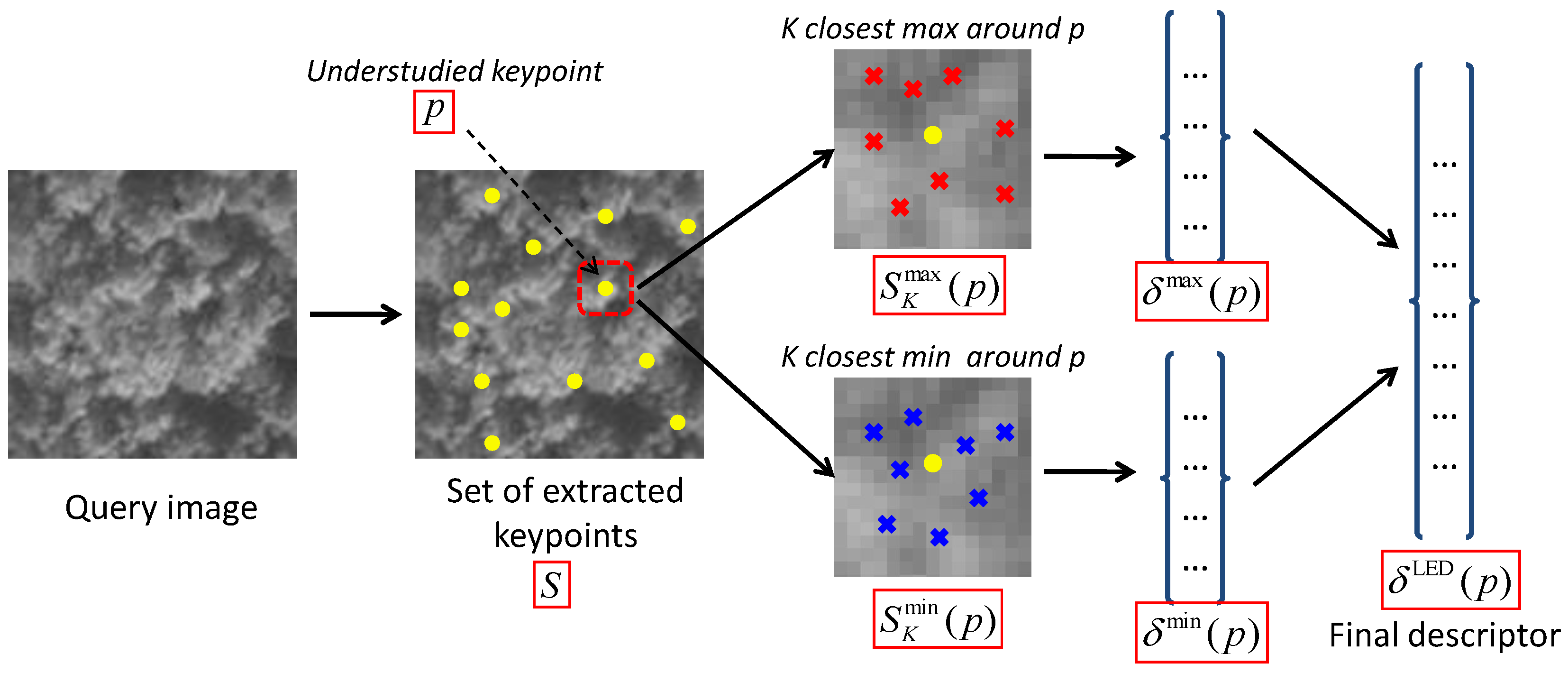
3.1. Extraction of the Local Extrema Descriptor

The idea is that, for each query image, we extract a set of characteristic points and then generate their local descriptors. Hence, the image is encoded by a set of local descriptors, which can be considered as a point cloud within the feature space. At this point, some popular feature extraction and description techniques, such as Harris corner points, scale-invariant feature transform (SIFT) or speeded up robust features (SURF) (cf. the review in [18]), may be prospective. Therefore, one may wonder about the possibility to use these feature points to perform our algorithm. In fact, the local extrema pixels are more suitable for texture representation and characterization. A texture can be considered as a spatial arrangement and distribution of pixels having some variation of intensity. Once there is a variation of intensity, there exists the local maximum and local minimum pixels. Hence, these local extrema can be extracted from all texture zones. Meanwhile, interest points, including Harris, SIFT or SURF, usually focus on image features, such as corners, edges and salient objects. They may not be detected within quite homogeneous regions, like bare soils, flat grass fields and early-growing vegetation areas. We illustrate in Figure 2 an example to clarify the irrelevance of those points compared to our proposed local extrema points. The figure shows the distribution of three types of keypoints, including the local extrema, Harris and SIFT points on the image plane. About 3000 points (marked in red) are detected in each case. From Figure 2c,d, we observe the lack of points from the homogeneous grass-field regions yielded by the Harris and SIFT techniques. In fact, these regions still involve a smooth texture, which needs to be characterized. If the Harris or SIFT keypoints are exploited for texture analysis, these texture zones will not be taken into account. Meanwhile, the proposed local extrema keypoints (Figure 2b) are detected from all image regions having an intensity variation to cover any texture. Hence, they are more relevant for the expected keypoint-based strategy for texture analysis.
We now recall the extraction of the local extrema points. For more details, readers are invited to consult papers [16,17]. A pixel in a grayscale image is supposed to be a local maximum (resp. local minimum) if it holds the highest (resp. lowest) intensity value within a neighborhood window centered at it. Let S ω max ( I ) and S ω min ( I ) denote the local maximum and local minimum sets extracted from a grayscale image I using the ω × ω search window. Let i = ( x i , y i ) be a pixel located at position ( x i , y i ) on the image plane with an intensity value I ( i ) ; we have:
i S ω max ( I ) I ( i ) = max j N ω × ω ( i ) I ( j )
i S ω min ( I ) I ( i ) = min j N ω × ω ( i ) I ( j )
where N ω × ω ( i ) represents a set of pixels inside the ω × ω neighborhood window around i. It is worth noting that only one parameter ω is required for the extraction of these local extrema. The value of ω decides the density of keypoints. Within a image texture, the higher ω is set, the fewer the number of keypoints that are detected.
Back to our strategy, Figure 3 highlights the feature extraction stage. For a query image, we extract a set of keypoints denoted by S. In this work, keypoints are the local maximum pixels. It is worth noting that using the local minimum pixels or both will provide similar performance. The important point is that for each keypoint p S , an LED δ LED ( p ) is generated to encode its structural and textural features. Considered as an improved version of the pointwise (PW) descriptor proposed in [14,15,16], the LED is constructed by incorporating both radiometric and geometric information of local maximum and minimum pixels around each central keypoint. Moreover, we propose to insert the gradient magnitude and orientation features of these local extrema to deal with very structured and oriented features given by the vine plot characteristics observed from VHR images.
Let us consider an understudied keypoint p located at position ( x p , y p ) having its intensity I ( p ) ; we firstly search for a set of K closest local maximum pixels and a set of K closest local minimum pixels from the two sets S ω max ( I ) and S ω min ( I ) , denoted by S K max ( p ) and S K min ( p ) , respectively (see Figure 3). The following features are extracted from the set S K max ( p ) , noting that a similar procedure will be applied to S K min ( p ) .
  • Mean and variance of intensities: μ I , σ I 2
  • Mean and variance of distances of every point from the set to the keypoint p: μ d , σ d 2
  • Measure of directional variance [19] of angles formed by these points and p: σ α 2
  • Mean and variance of gradient magnitudes: μ g , σ g 2
  • Measure of the directional variance [19] of gradient orientations: σ θ 2
Denote δ max ( p ) the feature vector generated from the closest maximum set S K max ( p ) around keypoint p; we have:
δ max ( p ) = [ μ I , σ I 2 , μ d , σ d 2 , σ α 2 , μ g , σ g 2 , σ θ 2 ] R 8
A similar process is applied to S K min ( p ) in order to generate δ min ( p ) . Finally, denote δ LED ( p ) the final LED descriptor of p; we insert the intensity I ( p ) to form it as follows:
δ LED ( p ) = I ( p ) , δ max ( p ) , δ min ( p ) R 17
The δ LED ( p ) descriptor allows us to characterize the local environment around each keypoint p. It helps to understand how the local maxima and the local minima are distributed and arranged and also how they encapsulate the spatial information, radiometric characteristics and structural properties (given by gradient features). Hence, it represents our proposed textural and structural feature descriptor. It is worth noting that LED descriptors are invariant to rotation. As observed from their calculation, for the two directional features, including the geometric angle α and the gradient orientation θ, only their directional variances [19] were taken into account. Their mean values were discarded to ensure the rotation-invariant property. In terms of feature dimensionality, an LED consists of 17 features. One may realize that this descriptor can be easily improved or adapted by modifying or adding other features into the vector in Equations (3) and (4). For example, one could insert more gradient features from different orientations. Others may include some multiscale features yielded by certain filtering processes, etc. The improvements will depend on one’s expectation to perform their own descriptor. Here, we basically propose three main types of features describing the radiometric, geometric and gradient properties in order to perform our own LED descriptor. The following sections in the paper will evaluate and validate its performance for retrieval and classification frameworks within the context of vineyard detection.

3.2. Dissimilarity Measure for Retrieval

Each image patch I i from the texture database is now characterized by a set of LED, which can be considered as an LED feature point cloud F i of size N i × 17 , where N i = | S i | is the number of keypoints extracted from I i :
F i = δ LED ( p ) p S i
We now compute the dissimilarity matrix involving all pair-wise distance measures for the database. Here, we propose to investigate two different distance measures: the simplified Mahalanobis distance and the Riemannian distance [20]. For its computation, the Mahalanobis distance takes into account the mean feature vector and the feature covariance matrix of each feature point cloud. On the other hand, the Riemannian distance focuses on the geometric structures of the two point clouds. Hence, it only considers the covariance matrix, not the mean feature vector, of each point cloud during its calculation. The estimations of the mean feature vector μ i and the feature covariance matrix C i of a point cloud F i are as follows:
μ i = 1 N i p S i δ LED ( p )
C i = 1 N i p S i δ LED ( p ) μ i T δ LED ( p ) μ i
Let us denote μ i , μ j , C i and C j the mean vectors and the feature covariance matrices estimated from the two feature point clouds F i and F j , respectively. The simplified Mahalanobis distance between I i and I j is computed as:
d mahalanobis ( I i , I j ) = d mahalanobis ( F i , F j ) = ( μ i μ j ) C i 1 + C j 1 ( μ i μ j ) T
and the Riemannian distance is calculated by:
d riemannian ( I i , I j ) = d riemannian ( F i , F j ) = = 1 d ln 2 λ
where λ is the -th generalized eigenvalue that satisfies λ C i χ C j χ = 0 ; = 1 , , d . χ is the corresponding eigenvector to λ , and d = 17 is the dimension of the LED feature vector.
Once the distance matrix is formed, a cross-validation approach with a random selection procedure is employed to evaluate the retrieval performance. At each iteration, an equal number of n images is randomly extracted for each class. Based on the distance matrix, n most similar images are considered for each query image. The retrieval rate is calculated as the percentage of images belonging to the same class as the query found in its n top matches. After a number of iterations, the average retrieval rate (ARR) can be computed and used to assess the algorithm performance.

3.3. Proposed Retrieval Algorithm

The outline of the proposed retrieval algorithm for VHR optical images can be found in Algorithm 1.
As observed from the algorithm, we propose that our keypoints are also the local maximum pixels extracted by a window size ω 2 . It should be noted that ω 2 can be set the same as or different from ω 1 . We usually set ω 2 ω 1 to get a coarser density of keypoints and to speed up the calculation time. More details about the sensitivity of the algorithm to ω 2 will be discussed in Section 3.5.
Algorithm 1: Proposed retrieval algorithm.
Remotesensing 08 00368 i001

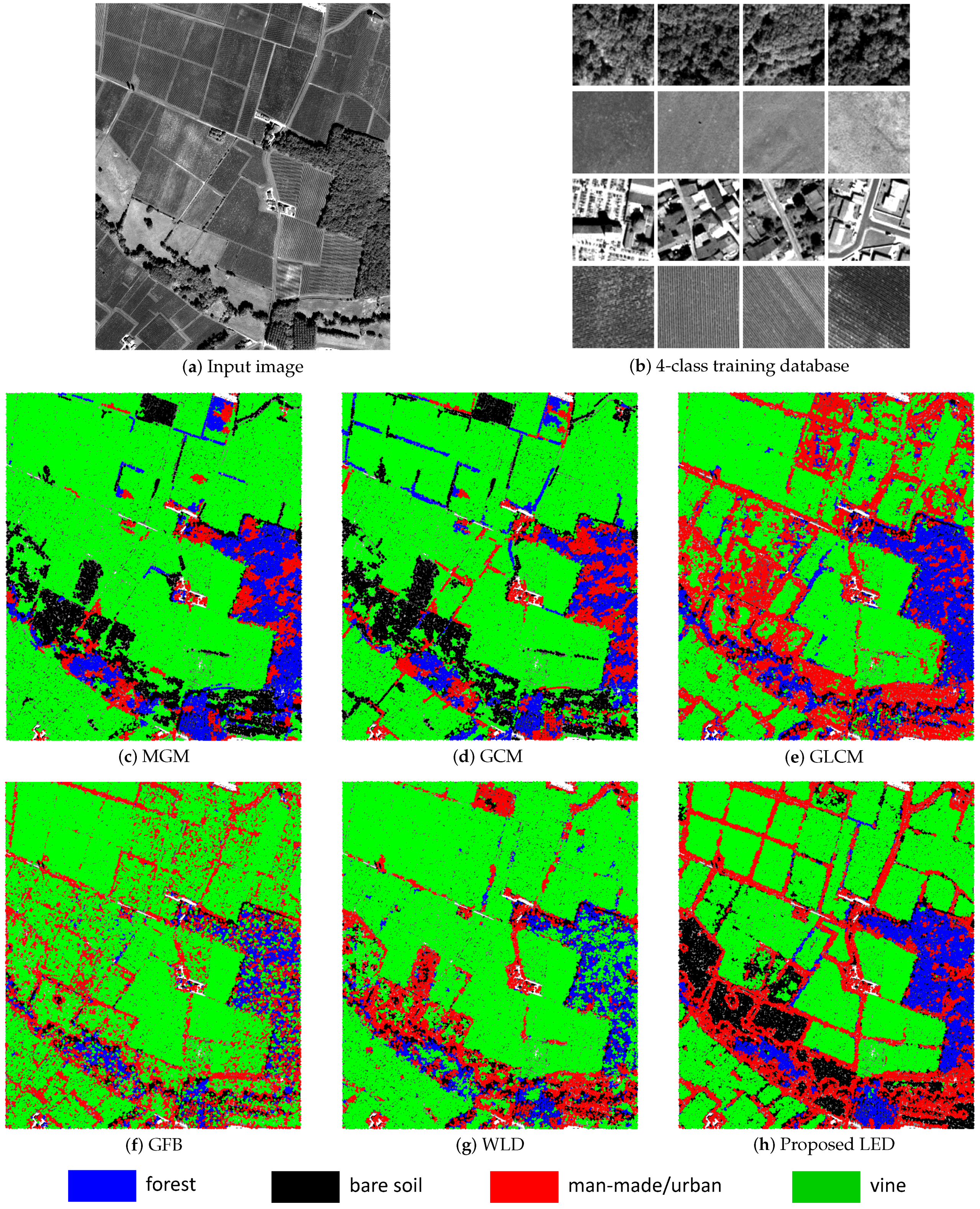
3.4. Retrieval Results

The proposed method is applied to the two databases described in Section 2 by following Algorithm 1. The number of image patches per class within each database can be found in Table 1. For parameter setting, local max and local min pixels are detected using a 3 × 3 search window ( ω 1 = 3 ). The local max keypoints are extracted by the 7 × 7 window ( ω 2 = 7 ). Here, we set ω 2 > ω 1 to accelerate the computational time, as mentioned in the previous subsection. Experiments show that ω 2 set from three to nine can bring quite similar retrieval performance. In terms of time consumption, the lower the value of ω 2 (i.e., higher density of keypoints), the greater the calculation time. Next, the number K of closest maxima and closest minima considered for each keypoint to generate its LED can be set from 10 to 30. We will show later that the results obtained by K equal to 15 and 20 are not significantly different. Moreover, a detailed analysis of the sensitivity of the proposed algorithm to parameters ω 2 and K in terms of ARR and computational time will be provided in Section 3.5.
For a comparative study, several reference methods are also implemented, including:
(1)
three statistical local texture descriptors: the gray-level co-occurrence matrix (GLCM) [1,5,6], the Gabor filter banks (GFB) [2,7,8] and the local Weber descriptor (WLD) [3,11]. The GLCM and GFB appear to be two of the most widely-used methods for texture analysis in remote sensing imagery. They have been adopted for the vine detection task within the last ten years [5,6,7,8]. Meanwhile, the WLD is one of the most recent local descriptors in computer vision;
(2)
three distribution models of wavelet coefficients: the multivariate Gaussian model (MGM), the spherically-invariant random vectors (SIRV) and the Gaussian copula-based model (GCM) [12,13]. These methods are the most recent wavelet-based techniques proposed for tackling texture-based retrieval and vine detection tasks. They are considered to give state-of-the-art retrieval performance for our two databases;
(3)
the pointwise (PW) descriptor proposed in our early work [16]. This descriptor only exploits the radiometric and spatial information from local extrema points. Gradient features are not considered. Our LED can be considered as the improved version of PW by integrating gradient features and taking into account the rotation-invariant property. The comparison to the PW descriptor allows us to validate the significant role of gradient features to characterize textural features in this study of vine cultivation.
We note that the implementations of the three model-based techniques (i.e., MGM, SIRV, GCM) are inherited from [12,13]. Then, the three statistical descriptors (GLCM, GFB, WLD) are implemented using a keypoint-based approach. They are generated only at keypoint positions to form dedicated feature point clouds, similar to the principle of our strategy. The objective is to perform an equivalent comparison to the proposed LED descriptor. Without loss of generality, the window size (W) set to compute these descriptors at keypoints is varied from 30 × 30 pixels to 50 × 50 pixels. Then, the window size that maximizes their performance is adopted. We note that the three wavelet-based techniques cannot be generated by such a keypoint-based approach, since they densely employ all pixels from the image to perform wavelet transform. Here are the implementations of the GLCM, GFB and WLD methods within a keypoint-based approach:
  • GLCM [1,5,6]: From the W × W neighborhood around each keypoint, compute four co-occurrence matrices along four main directions ( 0 , 45 , 90 and 135 ) with the distance between pairwise pixels set to two and the number of gray levels set to eight, then extract five Haralick textural parameters for each matrix including the contrast, correlation, homogeneity, energy and entropy in order to create the 20-feature GLCM descriptor for each keypoint.
  • GFB [2,7,8]: Perform the Gabor filtering on the image by setting the number of scales to three and the number of orientations to eight. The window size of a 2D filter kernel is equal to W × W pixels. Then, 24 features from the filter responses are adopted to create the GFD descriptor for each keypoint.
  • WLD [3,11]: Following the related paper, the differential excitation ξ and the quantized gradient orientation Φ for the image are first calculated using the 3 × 3 neighborhood. A 2D histogram H ( ξ , Φ ) is constructed for the W × W window around each keypoint. Then, the 1D WLD descriptor is generated by setting M = 6 , T = 4 and S = 3 (dedicated parameters of WLD; see [3]). Therefore, the dimension of WLD is 72.
Table 2 shows the texture retrieval performance on the two databases yielded by the proposed algorithm compared to reference methods. Here, the last four rows present four combinations of the proposed LED strategy by setting K equal to 15 or 20 and using the simplified Mahalanobis distance in Equation (8) or the Riemannian distance in Equation (9). In our implementation, the cross-validation procedure is activated by setting T = 100 iterations and n = 25 images/class for each iteration. We observe that the proposed approach provides the best ARR for both datasets with an ARR equal to 85 . 79 % for Pessac 22-08-12 and 89 . 43 % for Emilion 03-09-13. In terms of the number K, a slightly better performance is achieved for K = 20 than for K = 15 , but not very significantly. This issue emphasizes the robustness of the LED to the number of local extrema considered during its construction. In addition, the Riemannian metric seems to perform more efficiently than the simplified Mahalanobis distance. Hence, we suggest that the retrieval process should take into account the Riemannian distance for dissimilarity measurement. On the other hand, the Mahalanobis distance will be in fact exploited in the next stage of supervised classification of the vine detection application. We explain this remark in more detail in the Section 4. Another important remark is that compared to the pointwise (PW) descriptor, the proposed LED has an ARR enhancement of 7 . 55 % for Pessac-22-08-12 and 6 . 25 % for Emilion-03-09-13, with the same parameter setting. This issue confirms the significant role of structural gradient features integrated into LED feature vectors.
Finally, in terms of per-class performance, Table 3 shows that the proposed approach can provide good performance for all classes. The per-class retrieval rates for both datasets appear quite homogeneous. In particular, it is very effective in retrieving local structural items, such as buildings, structured forests and aligned vine rows. The reason is that we have focused on characterizing local textural features within VHR images and taken them into account during the construction of our proposed LED descriptor. Our method reaches the best retrieval rate for urban and vine classes (i.e., 95 . 97 % and 78 . 34 % for Pessac; 98 . 87 % and 77 . 69 % for Emilion). Within the two databases, there exists a confusion between the bare soil and vine classes. This is caused by some homogeneous or mitigated textures from low-spacing vine fields. Furthermore, some damaged or dead vines destroy the aligned structures of vine rows. That is why the retrieval rates on bare soil and vineyard classes are more limited than for forest and urban classes. As mentioned in Section 2, from the Pessac site, most of the vine parcels have low spacing rows (close to 1 m). This introduces smoother vine textures similar to bare soils. The result on bare soil for this site is hence decreased (i.e., 77 . 75 % compared to 85 . 69 % for Emilion). Therefore, the total ARR is lower ( 85 . 79 % compared to 89 . 43 % ). Related to the performance of reference approaches, the wavelet-based techniques, including MGM and GCM (the first two columns), achieve very good performance on forest and bare soils. On the contrary, they yield poor results on urban and vine classes. For example, MGM can produce 96 . 51 % for forest, 95 . 76 % for bare soil, but only 43 . 99 % for vineyard (for the Pessac database). This reduces its overall ARR ( 77 . 51 % compared to 85 . 79 % yielded by our method). The same remark can be given for the GCM method. The reason is that the forest zones and bare soils induce very homogeneous textures (i.e., stationary), which is appropriated for the Gaussian models considered by these methods. Meanwhile, in urban zones and vine fields, the notion of local textures and structures is more significant. It would not be relevant to model these two classes by multivariate Gaussian distributions. In conclusion, Table 3 shows that the proposed method can provide homogeneous results for all classes. More importantly, it satisfies our first goal of retrieving structural and textural items from the scene, especially vine-plot structures. This issue ensures a good preparation for the next stage of vine parcel detection by a supervised classification scheme.

3.5. Sensitivity to Parameters

This subsection aims at studying the sensitivity of the proposed retrieval framework to its parameters. As observed from the full retrieval algorithm (Algorithm 1) in Section 3.3, three main parameters are required in our framework, including: the window size to detect local maximum and local minimum pixels ( ω 1 ), the window size to extract local max keypoints ( ω 2 ) and the number of closest extrema taken into account for each keypoint to construct LED descriptors (K). Since ω 1 needs to be small enough to ensure sufficiently dense local extrema to support the computation of LED, we propose to fix it to 3 × 3 pixels in this work. Hence, only two parameters are considered to influence the performance of our method: ω 2 and K. We now investigate the sensitivity of the algorithm to each of them.
Figure 4a shows the performance of the proposed algorithm obtained by fixing ω 1 = 3 , K = 20 and varying ω 2 from three to 11. Experiments are performed on the Emilion 03-09-13 data. We note that using the Pessac 22-08-12 data provides a similar observation. First of all, a decrease in ARR from 89 . 99 % to 87 . 32 % is observed when ω 2 increases from three to 11. This remark can be explained as follows. As previously discussed in Section 3.3, the higher ω 2 , the coarser the density of keypoints. When the number of keypoints N i considered for each image I i decreases, the estimation accuracy of the feature covariance matrix C i in Equation (7) is reduced. The calculation of Riemannian distance (Equation (9)) is thus influenced. In other words, the more keypoints we use to characterize the image, the more precisely the covariance matrix is estimated, and hence, a higher ARR is obtained. Nevertheless, since only a decrease of 1 . 03 % (from 89 . 99 % to 88 . 96 % ) is yielded when ω 2 switches from three to nine, the method can be considered to be less sensitive to parameter ω 2 . Next, in terms of computational cost, the LED feature extraction time per image patch is significantly reduced when ω 2 increases. This is also because a fewer number of keypoints is exploited. Hence, we can conclude that ω 2 involves a compromise between the accuracy of covariance matrix estimation and the rapidity of LED feature extraction. Thus, it leads to a compromise between the retrieval rate and the calculation time of our algorithm. To this end, although the best performance in ARR ( 89 . 99 % ) is obtained by setting ω 2 = 3 , one may prefer setting it to five or seven to speed up the computation time (i.e., as our parameter setting with ω 2 = 7 in Section 3.4). Indeed, by setting ω 2 = 7 , we gain about 55 % of time (i.e., reduced from 0 . 886 s to 0 . 396 s per image). However, only a reduction of 0 . 56 % in ARR (i.e., from 89 . 99 % to 89 . 43 % ) results.
Similarly, the algorithm sensitivity to the parameter K (i.e., the number of closest extrema considered for each keypoint for the generation of its LED) can be found in Figure 4b. Here, we fix ω 1 = 3 , ω 2 = 7 and vary K from 10 to 30. Firstly, a stable performance can be observed with an ARR varying from 88 . 6 % to 89 . 43 % . The variation involves two stages. When K increases from 10 to 20, ARR is enhanced to reach the highest value ( 89 . 43 % ). Then, if K continues to increase from 20 to 30, ARR starts to be reduced. Here is our explanation. The parameter K in our strategy plays a similar role to that of the sliding window W × W set for the construction of classical dense descriptors. Hence, it has a similar behavior. At the first stage, when K increases, more information of the local neighborhood (i.e., which includes K closest maxima and K closest minima) around the keypoint is taken into account. Thus, the performance of the LED is improved. If we continue to increase the value of K, the equivalent support neighborhood size becomes larger and larger. Although more information is exploited, we may lose the notion of local feature and signal stationarity. This reduces the capacity of the LED to discriminate local structures and textures. Hence, the retrieval performance is decreased. In terms of computational time, the greater the number of extrema considered for each keypoint, the greater the calculation time. In general, at K = 20 , only a total time of 389 . 65 seconds is necessary for the complete algorithm to produce 89 . 43 % retrieval accuracy for 984 patches of the Emilion 03-09-13 database. This issue makes the proposed strategy very effective and competitive in both retrieval performance and computational cost. In conclusion, the two figures in Figure 4a,b show that the proposed LED method is not very sensitive to its parameters. A stable performance can be adopted with a wide range of parameters: ω 2 { 3 , , 9 } and K { 10 , , 30 } .

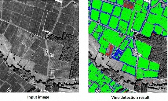
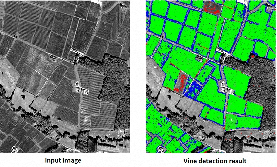
4. Application to Vineyard Parcel Detection

4.1. Supervised Classification Algorithm

In the previous section, the proposed LED has proven its capacity to characterize local structural and textural features from VHR images. Its performance has been validated for a texture-based image retrieval system with very promising and competitive results. We now tackle the main purpose of vineyard parcel detection based on VHR satellite images. As stated at the beginning of the article, we would like to perform a supervised classification algorithm to distinguish vine parcels from others classes present from the image content, such as forest zones, bare soils and urban areas. Here, only keypoints are exploited for classification, not all pixels from the image. In detail, the following algorithm (Algorithm 2) is activated with the helps of the k -nearest neighbor (kNN) classifier [21] and Mahalanobis distance:
Algorithm 2: Proposed supervised classification algorithm.
Remotesensing 08 00368 i002
The computation of the distance d ( p , I i ) from each keypoint p S to the image patch I i in the training set is defined as follows:
d ( p , I i ) = d Mahalanobis ( δ LED ( p ) , F i ) = δ LED ( p ) μ i C i 1 δ LED ( p ) μ i T
where μ i and C i are the mean feature vector and the feature covariance matrix estimated for the point cloud F i as in Equations (6) and (7).
We note that the Mahalanobis distance is exploited here, since it can be measured from one sample feature point δ LED ( p ) to the point cloud F i . On the other hand, the Riemannian metric is not applicable, since it is a distance between two point clouds whose covariance matrices are both required for its computation as in Equation (9). Hence, it is more relevant for the texture retrieval task when the distance between two image patches needs to be computed.

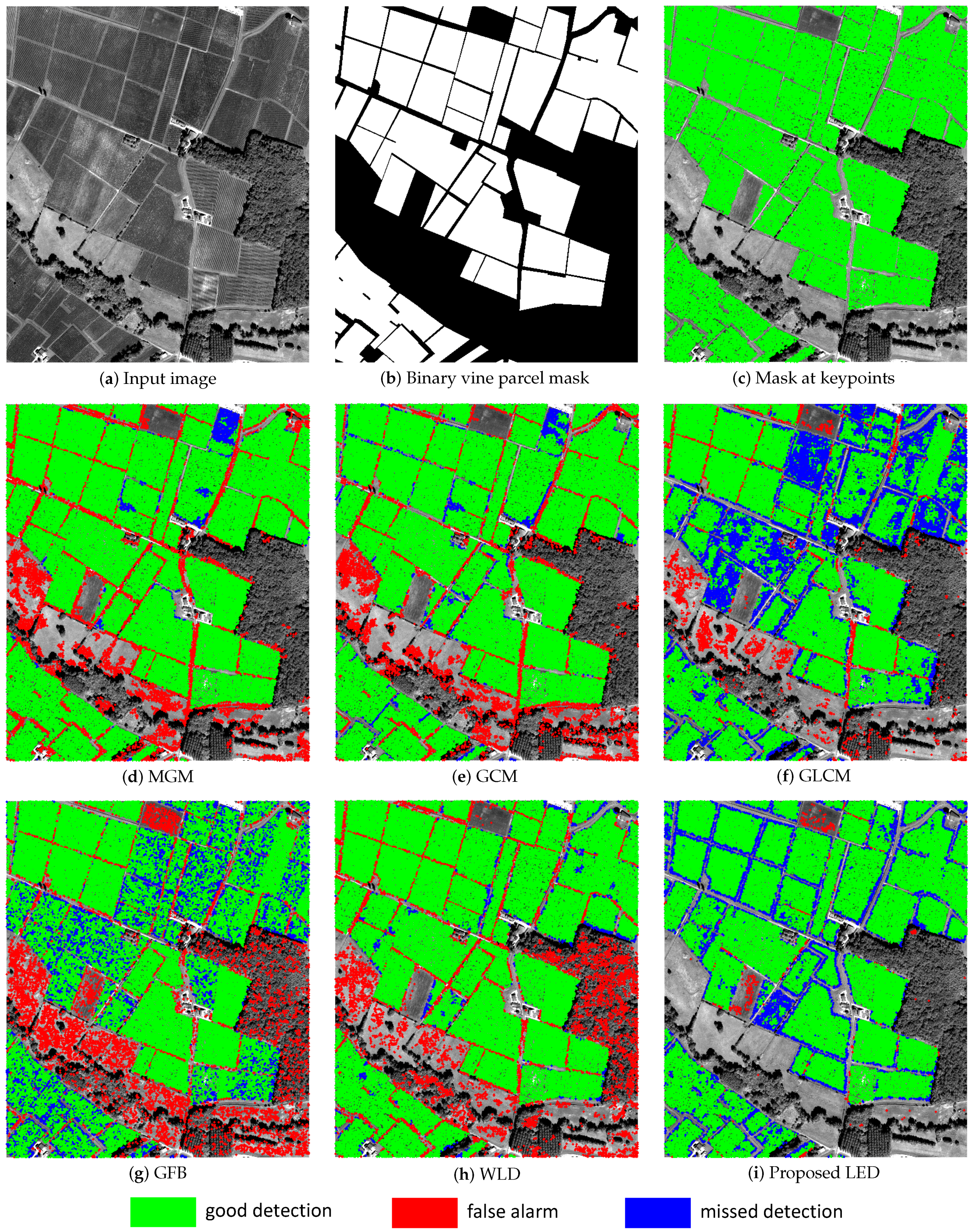
4.2. Evaluation Criteria

It should be noted that our main objective is the detection of vine parcels within the image. Since we do not have a full four-class classification ground truth, classification performance cannot be quantitatively evaluated. A binary ground truth mask for vineyard locations is available. Hence, we are interested in a detection problem with only two primary classes: vine and non-vine (i.e., which consists of all remaining classes, including forest zones, urban/man-made areas and bare soils). For the performance evaluation of the proposed method compared to reference methods, both qualitative and quantitative assessments are performed. In order to generate certain evaluation indicators, let us remind about some quantities resulting from a detection procedure:
  • true positives (TP): the number of vine points correctly detected (i.e., good detections),
  • true negatives (TN): the number of non-vine points correctly detected,
  • false positives (FP): the number of non-vine points incorrectly detected as vine (i.e., false alarms),
  • false negatives (FN): the number of vine points incorrectly detected as non-vine (i.e., missed detections).
Now, let N be the total number of keypoints considered for the detection algorithm and N v i n e and N n o n v i n e be respectively the number of vine points and non-vine points from ground truth. We have N v i n e + N n o n v i n e = N . The following indicators are used for the evaluation:
  • ratio between the number of good detections (GD) and bad detections (BD) including false alarms (FA) and missed detections (MD):
    R = T P F P + F N
  • percentage of total errors (TE) consisting of false alarms and missed detections:
    P T E = F P + F N N × 100 %
  • percentage of overall accuracy (OA):
    P O A = T P + T N N × 100 %

4.3. Experimental Results

This subsection describes our experimental setup and provides classification and detection results yielded by the proposed strategy compared to several reference methods. The proposed classification algorithm (Algorithm 2) was applied to a crop of 2000 × 1700 pixels extracted from the VHR panchromatic image acquired in the Saint-Emilion region. The image crop is shown in Figure 5a. As for the retrieval experimental study in Section 3.4, similar parameters were used for the generation of LED: ω 1 = 3 , ω 2 = 7 and K = 30 . Then, the kNN classification was used by setting k = 10 nearest neighbors. The Emilion 03-09-13 database with 984 image patches (see Table 1) was exploited as the training set. A total time of about 30 minutes was taken by the full algorithm using a basic MATLAB implementation on a machine with Core i7-3740QM 2.7 GHz, 16 GB RAM.
Figure 5 and Figure 6 provide the supervised classification and vine detection results yielded by the proposed LED descriptor compared to several reference methods. Here, we show the results produced by two wavelet-based techniques: the multivariate Gaussian model (MGM) and the Gaussian copula model [12,13]; and three classical statistical methods: the gray-level co-occurrence matrix (GLCM) [1], the Gabor filter banks [2] and the Weber local descriptors (WLD) [3]. The implementations of these reference methods were carried out similarly to the previous retrieval task. The supervised classification procedure was performed with parameters dedicated to each method to ensure an equivalent comparison. As observed in Figure 5, the proposed strategy produces well-separated classes from which vineyard parcels are discriminated from other classes (see Figure 5h). The classification process takes into account the boundaries (i.e., which are in fact dirt roads or ridges) between vine parcels and considers them to be similar to urban/man-made items (marked in red). On the other hand, the two wavelet-based techniques (Figure 5c to Figure 5d) and the WLD (Figure 5g) over-smooth these boundaries and provide quite homogeneous vine fields. Hence, they create over-detection results for vineyard class (i.e., most ridges are detected as vines). In terms of scene interpretation, we believe that it is better to classify these roads as man-made items than to detect them as vines. The result in Figure 5h enables us to recognize different vine parcels. Meanwhile, by over-detecting those ridges as vines, a many false alarms result. Hence, the detection performance will be reduced. The two other approaches including the GLCM and the GFB give poorer classification results in which some classes are mixed and vine fields are not well distinguished. Since we do not have a precise classification ground truth for all classes, only qualitative assessment for scene interpretation can be performed from Figure 5. Meanwhile, for vine detection task, a full qualitative and quantitative comparison will be provided.
In Figure 6, vine detection results are shown in which good detection (GD) points are marked in green, while false alarm (FA) and missed detection (MD) points are in red and blue, respectively. Again, the results obtained from GLCM (Figure 6f) and GFB (Figure 6g) are not sufficiently good with a great number of FA and MD points. The other results involve a compromise between the number of FA points and the number of MD points. The two wavelet-based approaches (i.e., MGM, GCM) and the WLD generate many FA points because of their over-detection problem. On the contrary, the proposed method produces more MD points. However, as observed from the figure, most of the MD points yielded by the proposed LED mostly come from boundary regions (i.e., dirt roads, ridges between vine parcels). This is because during the classification process, our method well detected these boundaries, but with a larger width, hence resulting in some missed vine points. In order to evaluate the performance of the proposed approach compared to the others, Table 4 provides some evaluation indicators described in the previous subsection. As observed from the table, the proposed algorithm provides the best detection result in terms of the ratio between good and bad detection points ( G D / F A + M D = 5 . 4971 ), as well as the percentage of total error ( P T E = 10 . 26 % ) and the percentage of overall accuracy ( P O A = 89 . 74 % ). An enhancement of 2 . 16 % is achieved compared to the best state-of-the-art method, the GCM with 87 . 58 % . Furthermore, compared to the PW descriptor, the proposed LED improves 2 . 22 % of the detection performance. Its again emphasizes the significant role of gradient features integrated into the descriptor.
Last, but not least, a similar classification framework was applied to a crop of 1300 × 1700 pixels extracted from the acquired image in the Pessac-Léognan region. The corresponding Pessac 22-08-12 database was employed as the training set. Table 5 provides the detection results yielded by the proposed LED compared to the reference methods. We note that this site involves more urban zones. More significantly, vine fields here appear more homogeneous, since their row spacing is small and close to the sensor resolution. For a reminder, the PLEIADES satellite’s spatial resolution at nadir is 0.7 m. The distance between vine rows at the Pessac-Léognan site is from 1 m to 1.2 m. In the Saint-Emilion region, this row spacing varies from 1.4 m to 2 m. Despite this challenge, the detection performance of all methods is quite similar to the previous case of the Saint-Emilion region. We again observe the best performance from the proposed LED descriptor with G D / F A + M D = 5 . 574 , P T E = 10 . 37 % and P O A = 89 . 63 % . An improvement of 2 . 67 % is made compared to the best reference method (GCM with P O A = 86 . 96 % ). In conclusion, the proposed method provides efficient and superior performance compared against all of the reference methods mentioned in the paper. It is evaluated and validated for both the texture retrieval task and the application of vine detection task. Its robustness is proven for both studied sites with different characteristics from the vine parcels.

5. Conclusions

A novel algorithm has been proposed to tackle the texture retrieval task in VHR imagery with an application to vineyard parcel detection. In the paper, the local extrema descriptor (LED) has been constructed to take into account textural and structural features from the image content. This non-dense approach based on characteristic points (i.e., local maximum and local minimum pixels in this work) is relevant in the scope of VHR images. Its performance has been evaluated and validated for both retrieval and supervised classification tasks using VHR panchromatic PLEIADES image data. As a conclusion, one can observe that the proposed LED descriptor is easy to build and implement, feasible to improve or extend and effective for VHR images when dealing with textural and structural items from the image. Future work can investigate the proposed strategy for other types of remote sensing image data, such as multispectral, hyperspectral or SAR images. Another perspective could be to improve the performance of the LED by exploiting and adding other features within its generation, which depends on one’s expectation and motivation to perform one’s own descriptor.

Acknowledgments

The authors would like to thank the French Space Agency (CNES) grant and the Brittany Region grant for funding this work. Also, we are grateful to Lionel Bombrun (University of Bordeaux) for his fruitful discussion.

Author Contributions

Minh-Tan Pham proposed the algorithm and performed the experiments under the supervision of Grégoire Mercier and Julien Michel. Olivier Regniers provided some prior concepts and the image data. Minh-Tan Pham wrote the paper, and Grégoire Mercier revised it. Julien Michel and Olivier Regnier gave comments and suggestions on the manuscript.

Conflicts of Interest

The authors declare no conflict of interest.

Abbreviations

The following abbreviations are used in this manuscript:
VHR
very high resolution
LED
local extrema-based descriptor
GLCM
gray-level co-occurrence matrix
GFB
Gabor filter bank
WLD
Weber local descriptor
MGM
multivariate Gaussian model
SIRV
spherically-invariant random vector
GCM
Gaussian copula-based model
SIFT
scale-invariant feature transform
SURF
speed up robust features
PW
pointwise
ARR
average retrieval rate
TP
true positives
TN
true negatives
FP
false positives
FN
false negatives
GD
good detection
BD
bad detection
FA
false alarm
MD
missed detection
TE
total error
OA
overall accuracy

References

  1. Haralick, R.M.; Shanmugam, K.; Dinstein, I. Textural features for image classification. IEEE Trans. Syst. Man Cybern. 1973, 3, 610–621. [Google Scholar] [CrossRef]
  2. Jain, A.K.; Farrokhnia, F. Unsupervised texture segmentation using Gabor filters. In Proceedings of the IEEE International Conference on Systems, Man and Cybernetics, Los Angeles, CA, USA, 4–7 November 1990; pp. 14–19.
  3. Chen, J.; Shan, S.; He, C.; Zhao, G.; Pietikäinen, M.; Chen, X.; Gao, W. WLD: A robust local image descriptor. IEEE Trans. Pattern Anal. Mach. Intell. 2010, 32, 1705–1720. [Google Scholar] [CrossRef] [PubMed]
  4. Van de Wouwer, G.; Scheunders, P.; van Dyck, D. Statistical texture characterization from discrete wavelet representation. IEEE Trans. Image Process. 1999, 8, 592–598. [Google Scholar] [CrossRef] [PubMed]
  5. Warner, T.A.; Steinmaus, K. Spatial classification of orchards and vineyards with high spatial resolution panchromatic imagery. Photogramm. Eng. Remote Sens. 2005, 71, 179–187. [Google Scholar] [CrossRef]
  6. Kayitakire, F.; Hamel, C.; Defourny, P. Retrieving forest structure variables based on image texture analysis and IKONOS-2 imagery. Remote Sens. Environ. 2006, 102, 390–401. [Google Scholar] [CrossRef]
  7. Delenne, C.; Rabatel, G.; Deshayes, M. An automatized frequency analysis for vine plot detection and delineation in remote sensing. IEEE Geosci. Remote Sens. Lett. 2008, 5, 341–345. [Google Scholar] [CrossRef] [Green Version]
  8. Rabatel, G.; Delenne, C.; Deshayes, M. A non supervised approach using Gabor filter for vine-plot detection in aerial images. Comput. Electron. Agric. 2008, 62, 159–168. [Google Scholar] [CrossRef]
  9. Ruiz, L.A.; Fdez-Sarría, A.; Recio, J.A. Texture feature extraction for classification of remote sensing data using wavelet decomposition: A comparative study. In Proceedings of the 20th ISPRS Congress, London, UK, 21 June 2004; pp. 1109–1114.
  10. Ranchin, T.; Naert, B.; Albuisson, M.; Boyer, G.; Astrand, P. An automatic method for vine detection in airborne imagery using the wavelet transform and multiresolution analysis. Photogramm. Eng. Remote Sens. 2001, 67, 91–98. [Google Scholar]
  11. Cui, S.; Dumitru, C.O.; Datcu, M. Ratio-detector-based feature extraction for very high resolution SAR image patch indexing. IEEE Geosci. Remote Sens. Lett. 2013, 10, 1175–1179. [Google Scholar]
  12. Regniers, O.; Da Costa, J.P.; Grenier, G.; Germain, C.; Bombrun, L. Texture based image retrieval and classification of very high resolution maritime pine forest images. In Proceedings of the 2013 IEEE International Geoscience and Remote Sensing Symposium—IGARSS, Melbourne, Australia, 21–26 July 2013; pp. 4038–4041.
  13. Regniers, O.; Bombrun, L.; Guyon, D.; Samalens, J.C.; Germain, C. Wavelet-based texture features for the classification of age classes in a maritime pine forest. IEEE Geosci. Remote Sens. Lett. 2015, 12, 621–625. [Google Scholar] [CrossRef]
  14. Pham, M.T.; Mercier, G.; Michel, J. Wavelets on graphs for very high resolution multispectral image segmentation. In Proceedings of the 2014 IEEE Geoscience and Remote Sensing Symposium, Quebec City, QC, Canada, 13–18 July 2014; pp. 2273–2276.
  15. Pham, M.T.; Mercier, G.; Michel, J. Textural features from wavelets on graphs for very high resolution panchromatic Pléiades image classification. Revue française de photogrammétrie et de télédétection 2014, 208, 131–136. [Google Scholar]
  16. Pham, M.T.; Mercier, G.; Michel, J. Pointwise graph-based local texture characterization for very high resolution multispectral image classification. IEEE J. Sel. Top. Appl. Earth Obs. Remote Sens. 2015, 8, 1962–1973. [Google Scholar] [CrossRef]
  17. Pham, M.T.; Mercier, G.; Michel, J. PW-COG: An effective texture descriptor for VHR satellite imagery using a pointwise approach on covariance matrix of oriented gradients. IEEE Trans. Geosci. Remote Sens. 2016, in press. [Google Scholar] [CrossRef]
  18. Tuytelaars, T.; Mikolajczyk, K. Local invariant feature detectors: A survey. In Foundations and Trends® in Computer Graphics and Vision; Now Publishers Inc.: Hanover, MA, USA, 2008; Volume 3, pp. 177–280. [Google Scholar]
  19. Mardia, K.V.; Jupp, P.E. Directional Statistics; John Wiley and Sons, Ltd.: Hoboken, NJ, USA, 2000; Volume 494. [Google Scholar]
  20. Förstner, F.; Moonen, B. A metric for covariance matrices. In Geodesy-The Challenge of the 3rd Millennium; Springer: Berlin, Germany, 2003; pp. 299–309. [Google Scholar]
  21. Cover, T.M.; Hart, P.E. Nearest neighbor pattern classification. IEEE Trans. Inf. Theory 1967, 13, 21–27. [Google Scholar] [CrossRef]
Figure 1. (a) The studied sites of the Pessac Léognan and Saint-Emilion regions, France. (b) Examples of four texture classes, including forest, bare soil, urban zones and vine fields (from top to bottom) extracted from the Emilion 03-09-13 database. (a) Studied sites; (b) Examples of four classes.
Remotesensing 08 00368 g001
Figure 2. Distribution of keypoints on the image plane: (a) Input 512 × 512 image; (b) local extrema points; (c) Harris corner points; (d) SIFT keypoints. In all cases, the number of keypoints is approximately 3000.
Remotesensing 08 00368 g002
Figure 3. Generation of local extrema descriptors (LED) for each query image.
Remotesensing 08 00368 g003
Figure 4. Sensitivity of the proposed retrieval framework to its parameters in terms of average retrieval rate (%) and LED feature extraction time (s). Experiments are performed on the Emilion 03-09-13 database using the Riemannian distance Equation (9). (a) Sensitivity to the window size ω 2 for keypoint extraction; (b) sensitivity to the number K of closest extrema for LED construction.
Remotesensing 08 00368 g004
Figure 5. Supervised classification results yielded by the proposed algorithm compared to reference methods. (a) Input 2000 × 1700 image. (b) Examples of training patches from the Emilion 03-09-13 database including 4 classes: forest, bare soil, urban and vine fields. (c)–(h) Classification results yielded by the multivariate Gaussian model (MGM), Gaussian copula model (GCM), Gray-level cooccurrence matrix (GLCM), Gabor filter bank (GFB), Weber local descriptor (WLD) and the proposed local extrema-based descriptor (LED) methods. Colored labels affected for the classes of forest, bare soil, man-made/urban and vineyard are blue, black, red and green, respectively. This figure is better visualized with colors.
Remotesensing 08 00368 g005
Figure 6. Vine parcel detection results yielded by the proposed algorithm compared to reference methods. (a) Input 2000 × 1700 image. (b) Binary map consisting of vine fields in white and non-vine fields in black. (c) Ground truth detection results at keypoints with vine points in green. (d)–(i) Detection results yielded by the multivariate Gaussian model (MGM), Gaussian copula model (GCM), Gray-level cooccurrence matrix (GLCM), Gabor filter bank (GFB), Weber local descriptor (WLD) and the proposed local extrema-based descriptor (LED) methods. Colored labels affected for Good detection (GD), False alarm (FA) and Missed detection (MD) points are green, red, blue, respectively. This figure is better visualized with colors.
Remotesensing 08 00368 g006
Table 1. Number of image patches per class within each database for the retrieval experiment.
DatabaseForestBare SoilUrbanVine FieldsTotal
Pessac 22-08-126653147179445
Emilion 03-09-13443227881984
Table 2. Retrieval performance on the two VHR texture databases using different methods in terms of average retrieval rate (ARR) ( % ) . MGM, multivariate Gaussian model; SIRV, spherically-invariant random vector; GCM, Gaussian copula-based model; GLCM, gray-level co-occurrence matrix; GFB, Gabor filter banks; WLD, Weber local descriptor; PW, pointwise.
MethodPessac 22-08-12Emilion 03-09-13
MGM77.5178.35
SIRV60.5860.16
GCM76.8875.91
GLCM54.5664.57
GFB61.3762.39
WLD64.3873.88
PW78.2483.18
LED (K = 15, Mahalanobis)83.4287.90
LED (K = 20, Mahalanobis)83.7888.18
LED (K = 15, Riemannian)85.6389.01
LED (K = 20, Riemannian)85.7989.43
Table 3. Per-class retrieval accuracy (%) yielded by different methods.
Class/MethodMGMGCMGLCMWLDPWLED (K = 20)LED (K = 20)
MahalanobisRiemannian
Equation (8)Equation (9)
Pessac 22-08-12
Forest96.5194.5461.6188.8479.0890.1292.37
Bare soil95.7692.4856.5361.7676.7674.9677.75
Urban73.7875.2848.3757.9783.0095.9794.64
Vineyard43.9942.2251.7548.9474.1374.0778.34
ARR77.5176.8854.5664.3878.2483.7885.79
Emilion 03-09-13
Forest93.7184.1279.2083.7390.8894.3597.93
Bare soil99.7196.2576.2678.8080.9983.8285.69
Urban86.9387.5152.8479.7388.5998.8796.40
Vineyard33.0539.7549.9653.2572.2875.6877.69
ARR78.3575.9164.5773.8883.1888.1889.43
Table 4. Comparison of the numbers of false alarms (FA), missed detections (MD), good detections (GD), the percentage of total errors ( P T E ) and the percentage of overall accuracy ( P O A ) produced by different methods. Experiments are performed on an image crop of 2000 × 1700 pixels acquired from the Saint-Emilion region with N vine = 32,853 points, N non-vine = 17,026 points.
MethodFAMDGD GD / (FA+MD) P TE P OA
(Points)(Points)(Points)(%)(%)
MGM601167632,1774.811913.4186.59
GCM5160103531,8185.136112.4287.58
GLCM2469820024,6532.310721.3978.61
GFB6316515927,6942.413423.0176.99
WLD602685831,9954.647713.8086.20
PW667555726,6964.289212.4887.52
Proposed412470828,1455.497110.2689.74
Table 5. Comparison of the numbers of false alarms (FA), missed detections (MD), good detections (GD), the percentage of total errors ( P T E ) and the percentage of overall accuracy ( P O A ) produced by different methods. Experiments are performed on an image crop of 1300 × 1700 pixels acquired from the Pessac-Léognan region with N vine = 18,176 points, N non-vine = 10,337 points.
MethodFAMDGD GD / (FA+MD) P TE P OA
(Points)(Points)(Points)(%)(%)
MGM2714149616,2303.482816.3483.66
GCM2309140816,7684.511213.0486.96
GLCM2010458913,5872.058923.1476.86
GFB2224574912,4271.558627.9672.04
WLD3704183616,3402.949519.4380.57
PW618469913,4772.534718.6581.35
Proposed1270168816,4885.574010.3789.63

