Improved Early Crop Type Identification By Joint Use of High Temporal Resolution SAR And Optical Image Time Series

Abstract

High temporal and spatial resolution optical image time series have been proven efficient for crop type mapping at the end of the agricultural season. However, due to cloud cover and image availability, crop identification earlier in the season is difficult. The recent availability of high temporal and spatial resolution SAR image time series, opens the possibility of improving early crop type mapping. This paper studies the impact of such SAR image time series when used in complement of optical imagery. The pertinent SAR image features, the optimal working resolution, the effect of speckle filtering and the use of temporal gap-filling of the optical image time series are assessed. SAR image time series as those provided by the Sentinel-1 satellites allow significant improvements in terms of land cover classification, both in terms of accuracy at the end of the season and for early crop identification. Haralik textures (Entropy, Inertia), the polarization ratio and the local mean together with the VV imagery were found to be the most pertinent features. Working at at 10 m resolution and using speckle filtering yield better results than other configurations. Finally it was shown that the use of SAR imagery allows to use optical data without gap-filling yielding results which are equivalent to the use of gap-filling in the case of perfect cloud screening, and better results in the case of cloud screening errors.

1. Introduction

Higher agricultural yields will be required in the future in order to fulfill food supply needs [1]. Added to this, bio-fuel production and urban growth are also increasing the pressure on agricultural lands [2,3,4]. All these factors will also have consequences on natural ecosystems [5,6].

In this context, crop area extent estimates and crop type maps provide crucial information for agricultural monitoring and management. Remote sensing imagery in general and, in particular, high temporal and high spatial resolution data as the ones which will be available with recently launched systems such as Sentinel-1 [7] and Sentinel-2 [8] constitute a major asset for this kind of application. We will use the term dense time series to refer to revisit rates which allow to capture the evolution of the signal of interest. In the case of crop type mapping, this corresponds to at least two images per month.

Recent works have shown that dense multi-temporal optical imagery as the one that will be provided by the Sentinel-2 satellites is able to provide accurate crop type mapping over different climates and diverse crop systems [9]. However, since optical imagery is affected by cloud cover, the performances of the crop type mapping system can be hindered in some cases, even with a 5-day revisit cycle. Furthermore, SAR data may improve the discrimination of some crop types which are difficult to distinguish with optical imagery alone.

Added to annual mapping as the one presented in [9], early crop type detection before the end of the season is needed for yield forecasting and irrigation management. Except for tropical or very arid areas, most of crop systems in the world have an annual cycle with possibly 2 sub-cycles (winter and summer crops). By early in the season we refer to the possibility of providing an annual crop type map between months 6 and 9 of the annual cycle. In this case, image availability and multi-sensor information is still more crucial.

Optical data is usually preferred to SAR imagery because of the better understanding of the link between the observations and vegetation phenology. However, the all-weather acquisitions provided by SAR and recent advances in the understanding of the underlying physical phenomena, make multi-temporal SAR imagery an interesting candidate for crop type mapping.

For instance, Skriver et al. [10] showed the interest of multi-temporal polarimetric signatures of crops. Schotten et al. [11] used ERS-1 multi-temporal data in order to perform field level classification to discriminate 12 crop types, achieving 80% accuracy. Their approach needed the selection of the best image subset among the 14 images available during the agricultural season.

Recently, Balzter et al. [12] showed that Sentinel-1 could be used to recognise some land cover classes of the Corine Land Cover nomenclature, although their study used only two dates and the results seemed to depend to a great extent on topography information.

The selection of optimal dates was also used by Skriver et al. [13] with the EMISAR airborne system which provided monthly polarimetric acquisitions achieving a 20% error rate for their particular study site.

In the perspective of an operational crop type map production system as the one presented for instance in [9], date selection is not possible and all available data has to be used.

The literature shows that in order to achieve high quality mapping results, full polarimetric SAR data is needed, although different authors came to different conclusions depending on their experiments. For instance, Moran et al. [14] concluded that full polarimetry with a revisit of 3 to 6 days is needed for crop identification and that with single or dual polarimetry, phenology is accessible, but crop type is not. On the other hand, Schotten et al. [11], found that the cross-polarised channel ${\sigma }_{\text{HV}}^{\text{0}}$ is correlated with NDVI for some crops, allowing for their identification.

Nowadays, the only satellite system providing full polarimetric SAR data is Radarsat-2, but due to its wide range of acquisition modes, it is difficult to obtain dense time series with global coverage.

Skriver et al. [15] found that multi-temporal SAR data provided a better trade-off than polarimetric imagery. Sentinel-1 does not provide full-polarimetric imagery. On the other hand, it will make available dense time series (6-day revisit cycle with two satellites), and it is therefore a good candidate for operational crop type mapping. McNairn et al. [16] investigated the possibility of early season monitoring for two classes (soybean and corn) using TerraSAR-X and Radarsat-2 time series. They highlighted the usefulness of multi-temporal speckle filtering.

Multi-sensor data fusion [17] approaches that combine SAR and high resolution optical sensors have clearly demonstrated an increased mapping accuracy.

SAR imagery for crop type mapping has been used together with optical data. For instance, McNairn et al. [18] used 2 SAR (Envisat-ASAR) images and one optical (SPOT4) to achieve acceptable accuracies. Zhu et al. [19] proposed a Bayesian formulation for the fusion of Landsat TM and ERS SAR (two images of each type). Their approach was based on building a specific statistical link between the two types of data for a particular set of acquisition dates, which is not general enough to be implemented in operational settings. However, their results showed the complementarity of the two types of data. The two works cited above used a small number of images. Sentinel-1 and Sentinel-2, with their short revisit cycle will offer improved possibilities.

Some works in the literature have already explored the use long time series, but they used a dense time series of one of the sensors (either optical or SAR) and a few images coming from the other modality.

For instance, Blaes et al. [20] used 15 SAR images (ERS and Radarsat) and three optical ones (Landsat TM). They performed a field level classification together with photo-interpretation schemes. They showed an improvement of the accuracy thanks to the use of SAR data, with respect to the accuracy achieved with three optical images. As most approaches in the literature, a date selection was used, which is incompatible with fully automatic operational systems.

Le Hégarat et al. [21] reached similar conclusions as [20] using other methods (Markov Random Fields and Dempster Shafer fusion). Their set up also used a SAR time series and only three Landsat images. They concluded that SAR SITS alone yields lower accuracies than three optical images alone, but that the synergy between the two types of data gives the best accuracy. Similar conclusions are reported by Chust et al. [22] using ERS and SPOT imagery and similar fusion methods.

Unlike the literature cited above, in this paper we assess the joint use of dense SITS of both SAR and optical imagery in order to devise a strategy for the operational exploitation of both Sentinel-1 and Sentinel-2 data in the frame of crop type mapping at early stages of the agricultural season. Several similar contributions have recently appeared in the literature. Forkuor et al. [23] investigated the contribution of X band polarimetric SAR images to crop mapping when used as a complement to high resolution optical SITS. Skakun et al. [24] investigated the use of C band Radarsat-2 dual polarimetric images together with Landsat8 time series as a preparation of the upcoming availability of Sentinel-1 images. However they used two different incidence angles and did not investigate the extraction of local features as textures or local statistics. Villa et al. [25] proposed an expert-based decision tree which is able to combine Landsat8 and X-band COSMO-SkyMed SAR image time series for in-season crop mapping.

Although these recent contributions give interesting and useful insights for the problem of crop mapping using optical and SAR SITS together, they do not address some key issues for the implementation of operational processing chains for early crop mapping. Indeed, the global availability of dense image time series makes Sentinel-1 data much more interesting than existing counterparts (Radarsat-2, TerraSAR-X, COSMO-SkyMed) for 2 main reasons:

• the images are available free of charge under an open license;
• the definition of a main acquisition mode (Interferometric Wide Swath) with constant viewing angles for the same point on the ground provides consistent time series with the same characteristics.

It is therefore interesting to investigate how to integrate these time series together with well known and used optical time series for crop mapping. In particular, it will be interesting to select the best image features and analyze the classification accuracy along the season in order to be able to provide early crop maps.

Similar approaches have recently been applied to forest monitoring mainly for tropical areas [26,27,28,29,30], but these approaches work in multi-year configurations which can not be applied for croplands, since the same field can change from one crop type to a different one in successive years.

The work on grasslands by Schuster et al. [31] showed the potential and complementarity of optical and SAR data for intra-year phenology monitoring, but the joint use of both sensor was not attempted.

The work presented here builds upon the results reported in [9], where the optical image exploitation work-flow was assessed. Therefore, the focus of the present work is on the integration of multi-temporal SAR data into the existing optical processing chain. In order to do that, the SAR image processing and feature extraction will be investigated. Since at the time of this writing Sentinel-2 has not reached its full acquisition capabilities, no time series covering a full crop season are available. In this work, we will use Landsat8 time series instead.

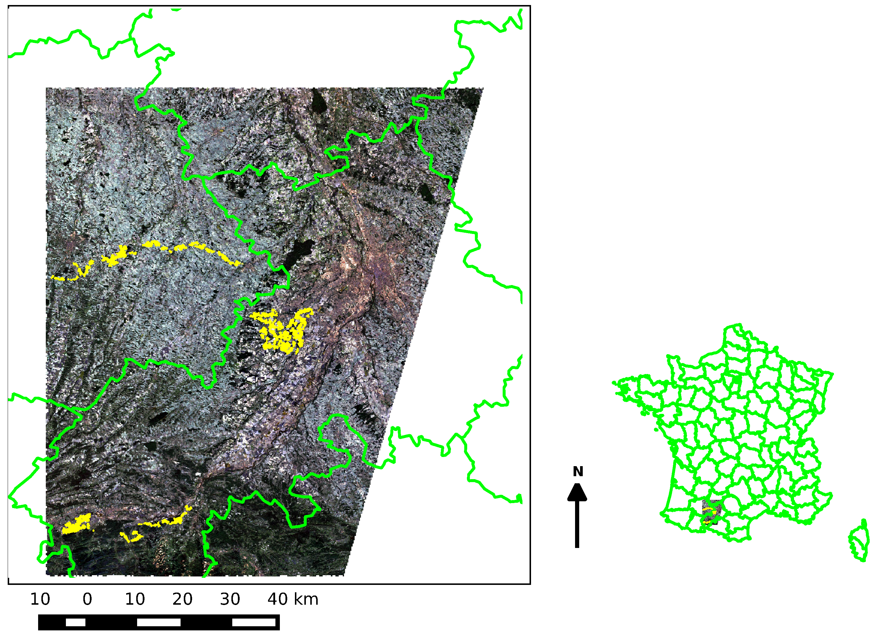
The paper is organized as follows. Section 2 introduces the study site and the data sets used. Section 3 describes the methodology applied and the different configurations used to assess the contribution of SAR time series to the crop type mapping quality. Section 4 presents the detailed results and discusses them. Finally, Section 5 draws final conclusion and suggests further research to improve the approach.

2. Data and Study Site

2.1. Reference Data

The study site is located in the south-west of France near Toulouse (Figure 1). The area is characterized by a temperate climate with an annual average temperature over 12 ${}^{\circ }$C, a minimum average for the coldest month over 2 ${}^{\circ }$C, and a maximum average over 10 ${}^{\circ }$C. The crop system is characterized by the use of a single crop per field each season. The annual season spans from October to September with a winter and a summer growing cycles. The 5 main crops in the area are wheat, rapeseed, barley (winter crops) and corn and sunflower (summer crops). Corn is usually used as a mono-culture (no rotation between years), while wheat and barley are grown alternating with rapeseed or sunflower [32].

A set of 1700 fields were surveyed on the ground on three different dates: in autumn before the soil work for the winter crop seeding, end of winter when winter crops were emerging and in mid-spring when summer crops started growing. A total of 1018 fields were kept after consistency checks between the three observations.

The land-cover classes in the reference data were: corn, wheat/barley, grass, bare soil, sunflower, rapeseed, alfalfa, soybean. The bare soil class corresponds to the summer crops which had not emerged at the date of the last survey.

Table 1. Number of fields and associated surfaces for each class in the reference data.

Class	Field Count	Total Surface (ha)	Minimum Field Size (ha)	Maximum (ha)	Median (ha)
Wheat/barley (WB)	302	1513.675	0.193	28.329	3.167
Bare soil (BS)	233	1165.905	0.057	36.035	2.758
Grass (GR)	263	613.315	0.079	19.765	1.575
Corn (CO)	90	387.998	0.114	22.298	3.260
Sunflower (SF)	59	356.543	0.102	30.826	4.495
Rapeseed (RA)	61	325.813	0.561	17.083	3.362
Alfalfa (AL)	7	14.155	0.277	3.805	1.968
Soybean (SO)	3	13.318	3.153	5.945	4.219

gives detailed information about the number of fields surveyed for each class in the reference data together with the total surfaces and statistics about the field sizes. As one can see, alfalfa and soybean are very rare in the area and the results will show that they are not recognized. They are however kept in the analysis in order to understand which are the classes they are confused with.

Non crop classes are not taken into account for the classification. A crop mask is produced using a supervised approach described in [33]. This approach needs samples of the non crop class, which are provided in our case by using the topographic data base of the French National Cartographic Institute.

2.2. Satellite Imagery

A set of 11 Landsat 8 [34] acquisitions were used as a surrogate of Sentinel-2 image time series. These images were processed to level 2A (i.e., surface reflectance values with masks for clouds, cloud shadows, snow and water) as described in [35].

Table 2. Landsat8 imagery used for this study.

Date	Path/Rows	${\mathrm{\Delta }}_{\mathit{days}}$	Cloud Cover (%)
01-09-2014	198/9-30		1.5
26-10-2014	199/29-30	55	0.4
20-11-2014	198/29-30	25	29.4
29-12-2014	199/29-30	39	7.1
14-01-2015	199/29-30	16	39.1
08-02-2015	198/29-30	25	73.3
12-03-2015	198/29-30	32	76.7
19-03-2015	199/29-30	7	58.6
13-04-2015	198/29-30	25	0.2
20-04-2015	199/29-30	7	60.1
29-04-2015	198/29-30	9	57.6

gives the list of the Landsat8 images used for this study together with the time gap between 2 consecutive acquisitions and the percentage of cloudy pixels on the study area.

Only 6 out of the 8 spectral bands at 30 m resolution were used (blue, green, red, NIR, SWIR1, SWIR2), since the coastal and the aerosol bands are not pertinent for vegetation mapping.

A set of 9 Sentinel-1 VV/VH SAR images (Interferometric Wide Swath, Ground Range Detected, IWS-GRD [36]) were radiometrically (antenna pattern correction) and geometrically corrected using the S1TBX software [37]. They were orthorectified on top of the Landsat imagery with a geometric accuracy estimated to be better than 30 m (1 Landsat pixel). No multi-looking was applied since the IWS-GRD products have an equivalent number of looks equal to 4.

Table 3. Sentinel-1 imagery used for this study.

Date	${\mathrm{\Delta }}_{\mathit{days}}$	Incidence Angle	Orbit
06-11-2014		39.047	DESCENDING
01-12-2014	25	38.821	ASCENDING
29-01-2015	59	38.965	DESCENDING
28-02-2015	30	38.909	ASCENDING
24-03-2015	24	38.939	ASCENDING
12-04-2015	19	38.886	ASCENDING
23-04-2015	11	39.000	DESCENDING
23-05-2015	30	38.913	ASCENDING
30-05-2015	7	38.968	ASCENDING

lists the acquisition dates, the time gap between two consecutive images, the incidence mean angle and the orbit type (ascending or descending). As one can see, one of the main features of Sentinel-1 is its acquisition plan with a main mode (Interferometric Wide Swath) which provides consistent time series in terms of incidence angles. The data set used for this study was acquired during the ramp-up phase of Sentinel-1 A and therefore, the full capacity of a 12 day revisit cycle with one satellite was not available yet.

Table 4. Acquisition dates and sensor type for the data used in this study.

Date	Sensor	${\mathrm{\Delta }}_{\mathit{days}}$
01-09-2014	Landsat8
26-10-2014	Landsat8	55
06-11-2014	Sentinel-1	11
20-11-2014	Landsat8	14
01-12-2014	Sentinel-1	11
29-12-2014	Landsat8	28
14-01-2015	Landsat8	16
29-01-2015	Sentinel-1	15
08-02-2015	Landsat8	10
28-02-2015	Sentinel-1	20
12-03-2015	Landsat8	12
19-03-2015	Landsat8	7
24-03-2015	Sentinel-1	5
12-04-2015	Sentinel-1	19
13-04-2015	Landsat8	1
20-04-2015	Landsat8	7
23-04-2015	Sentinel-1	3
29-04-2015	Landsat8	6
23-05-2015	Sentinel-1	24
30-05-2015	Sentinel-1	7

lists the available imagery for this study showing that the use of both sensors allows to reduce the average time gap between acquisitions from about 25 days (25.6 for Sentinel- and 24 for Landsat8) to 14.26 days. This revisit cycle will be very much improved when both Sentinel-1 and Sentinel-2 systems reach their full acquisition capabilities.

3. Methodology

As stated in the introduction, the goal of this study is to assess the usefulness of Sentinel-1 SITS for early crop type classification in complement to high resolution optical SITS. With this objective, several issues were analysed and are described below.

3.1. Incremental Classification

In order to perform crop type identification early in the agricultural season, an incremental classification procedure is used. It consists of performing a supervised classification every time that a new image acquisition is available using all the previously available imagery. In the case of this work, every new acquisition, either optical or SAR, triggers a new classification.

This set-up allows to analyze the evolution of the mapping quality as a function of time and therefore determine at which point in time the crop identification reaches an acceptable quality.

The validation protocol uses 50% of the reference data for training and the rest for the validation. The split between the 2 sets is performed at the field (polygon) level in order to ensure that a pixel from a field used for the training step is not used for the validation. Ten random splits are performed in order to perform 10 trainings and 10 corresponding validations, allowing to compute average performances with confidence intervals. In this paper the values of the κ coefficient [38] for the different settings will be reported.

The supervised classifier used is the Random Forest algorithm available in the Orfeo Toolbox (version 5.0) free software [39]. The rationale for this choice is described in [9] and can be summarised by the fact that Random Forests yield high quality mapping for a different variety of crop type systems for a much faster computation when compared to other state of the art classifiers as for instance Support Vector Machines with Gaussian kernels [40].

Rodríguez Galiano et al. [41] have showed that Random Forests classifiers have low sensitivity to parameters once the number of trees and their depth is large enough. In our case, the number of trees was set to 100 and their maximum depth to 25 (although most of the trees yield smaller values). The node splitting is done using the Gini impurity index evaluated on a random subset of features of size equal to the square root of the total number of features. Nodes are split if they contain more than 25 samples. This set of parameters was selected using a grid search approach.

3.2. Feature Selection

One of the critical issues for the use of SAR SITS is the choice of the features used for the classification. Tso et al. [42] found that SAR-based textures (ERS1) contributed little to crop discrimination, while filtered images produced the best result. We chose to reproduce this kind of analysis in order to investigate the contribution of polarimetric information which was absent in Tso’s work.

3.2.1. Evaluated Features

The main drawback of texture features is the computational complexity involved, which can be very important for SITS. Therefore, the feature selection has to take into account the trade-off between quality and computation time. Three families of texture measures were selected: statistical moments computed in a neighbourhood of each pixel, Haralik textures [43] and the Structural Feature Set [44] .

These texture features were added to the image intensity for each polarimetric channel as well as the ratio between the intensities of the VH and VV polarizations, $I_{VH}/I_{VV}$.

Table 5. SAR textures computed for every date in the time series.

Family	Feature Name
Local moments	mean
$3\times 3$ pixel window	variance
	skewness
	kurtosis
Haralik [43]	energy
$5\times 5$ pixel window	entropy
1 pixel offset in both directions	correlation
	inverse difference moment (IDM)
	inertia
	cluster shade
	cluster prominence
	Haralik’s correlation
SFS [44]	length
	width
	PSI
	w-mean
	ratio
	sd

gives the complete list of SAR image features computed for each available date.

For the optical data, the feature selection analysis was done in [9] and showed that the spectral reflectances, the NDVI (normalised difference between near-infrared and red [45]), the NDWI (normalised difference between green and near-infrared [46]) and the brightness index were able to grasp the most important information in the optical time series. Therefore, in this work, the feature selection method was only performed for the SAR features.

3.2.2. Feature Selection Method

The feature selection algorithm is based on the variable importance of the Random Forest classifier [47]: in every tree grown in the forest, the out of bag samples are classified using random permutations of each variable and computing the increase of classification errors with respect to the case without permutation. The average of this number over all trees in the forest is the importance score for each variable. This indicator has been found to be a reliable one [48,49], although it can yield to over-estimations for highly correlated variables [50]. The implementation in the Scikit-Learn software version 0.17 [51] was used.

Similar results were obtained using an uni-variate approach based on the analysis of the variances, but are not reported here for the sake of brevity. Recursive feature elimination [52] was not considered because of its computational complexity for a very high number of features, which was the case in this study.

In addition, since the classifier is chosen, using a selection method which is based on the same classifier allows to select features which will perform well with it.

One important point to bear in mind is that no date selection is performed. As stated in the introduction, in the frame of an operational system, all available information has to be taken into account. Also, in the case of crop monitoring, different dates are key for different crops. Finally, since the crop calendar changes across eco-climatic regions, conclusions about date selection may not be general.

Therefore, the contribution of a feature is analyzed as a whole in the time series. Furthermore, in order to take into account the trade-off between computational time and quality, textures will be selected per families. Indeed, the computational cost of Haralik features lies mostly in the computation of the grey-level co-occurrence matrices which are computed once for all textures. In the same way, the SFS computational cost comes from the construction of the directional histograms which are computed once for all the features of the family. Finally, statistical moments can also be computed with an efficient approach when several orders are needed [53].

3.3. Image Resolution and Speckle Filtering

Since the 2 sensors being used have different spatial resolutions (30 m for Landsat and 20 m × 22 m resampled to 10 m for Sentinel-1), a common resampling grid needs to be chosen for the joint use of the image time series. Both time series were ortho-rectified to the same cartographic projection (RGF93/Lambert-93, EPSG:2154) with an accuracy better than 30 m. Both the Landsat 30 m ground sampling and the Sentinel-1 10 m one were compared. These configurations are specific to the coupling of Sentinel-1 and Landsat8 SITS, but the conclusions may be applicable also to the case of Sentinel-1 with Sentinel-2, since the latter has spectral bands with different spatial resolutions ranging from 10 m to 60 m.

SAR images are contaminated by speckle noise. The use of speckle filtering applied to the Sentinel-1 data was therefore evaluated. A simple Lee with a filter $3\times 3$ pixel window was applied [54]. Contextual classification approaches robust to speckle for SAR imagery exist [55,56,57] but they are computationally expensive and have not been assessed in high dimensionality, as it is the case of SITS. Indeed, in our case, the number of features in the classification can easily exceed 100 (20 dates and several image features per date).

Although McNairn et al. [16] showed that multi-temporal speckle filtering improved crop classification, it was not used in this work because of 2 reasons:

• we use ascending and descending orbits and therefore opposite geometries between two subsets of images;
• except for two images, time gaps between consecutive images are greater than 19 days (see Table 3), and therefore, important evolutions of the back-scatter coefficient can occur.

3.4. Temporal Gap-Filling

One of the expected contributions of SAR SITS is the availability when optical data suffers from cloud cover. In the optical processing chain described in [9], a temporal gap-filling of the cloudy pixels was performed. Although the Random Forest classifier is known for its robustness to noisy data, the presence of clouds impacts the quality of the classification.

The last column of Table 2 shows that in some periods of the year, the cloud cover can be important. SAR imagery is expected to be useful in these periods, but a comparison with a simple gap-filling approach applied to optical time series has to be assessed. The same approach used in [9], which consists of a linear interpolation of the cloudy pixels using the previous and following cloud-free dates, was used here. On the other hand the gap-filling in itself can produce artefacts as it relies on the quality of the cloud screening approach.

4. Results and Discussion

In this section, we report the results of the experiments described in Section 3.

4.1. Feature Selection

The feature selection approach described in Section 3.2 was applied in order to sort the different SAR features by importance. The reader must bear in mind that no feature selection is applied on the features extracted from the optical images, but that all features (optical and SAR) are used in the importance computation. This allows to select the SAR features as a complement to the optical SITS. The use of SAR features alone might yield different results.

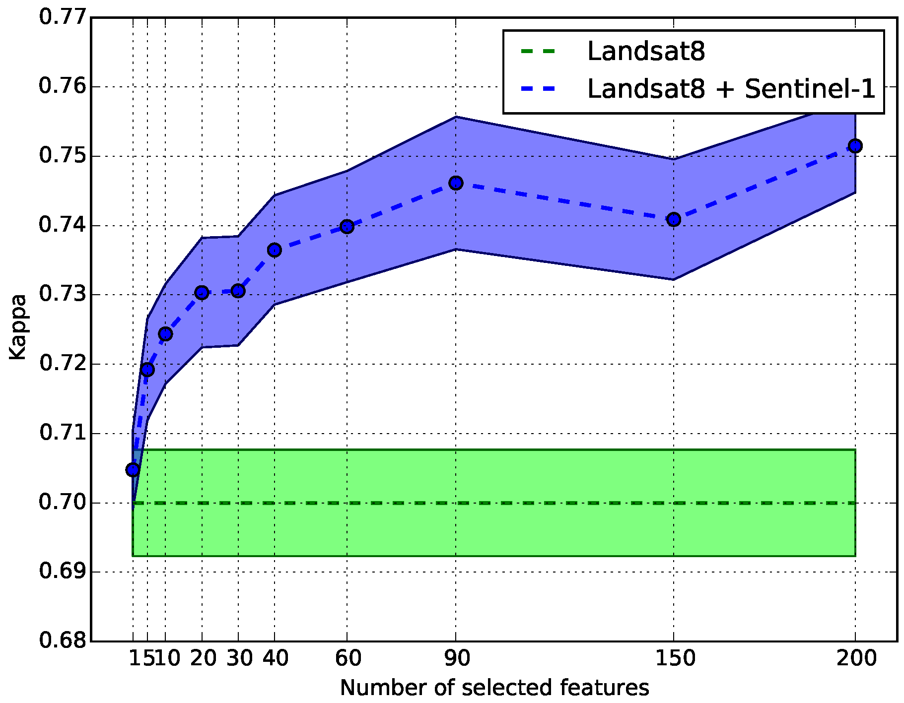
Figure 2 shows the evolution of the classification accuracy as a function of the number of SAR features selected. For this experiment, the complete time series was used and features were added in decreasing order of importance. One can observe that the first 20 most important features allow to achieve an increase of about 3 percentage points of κ. The improvement continues up to 60 features, although slowly and stabilizes afterwards.

As a trade-off between accuracy and computational cost, we choose to keep the 40 most important features in the following experiments.

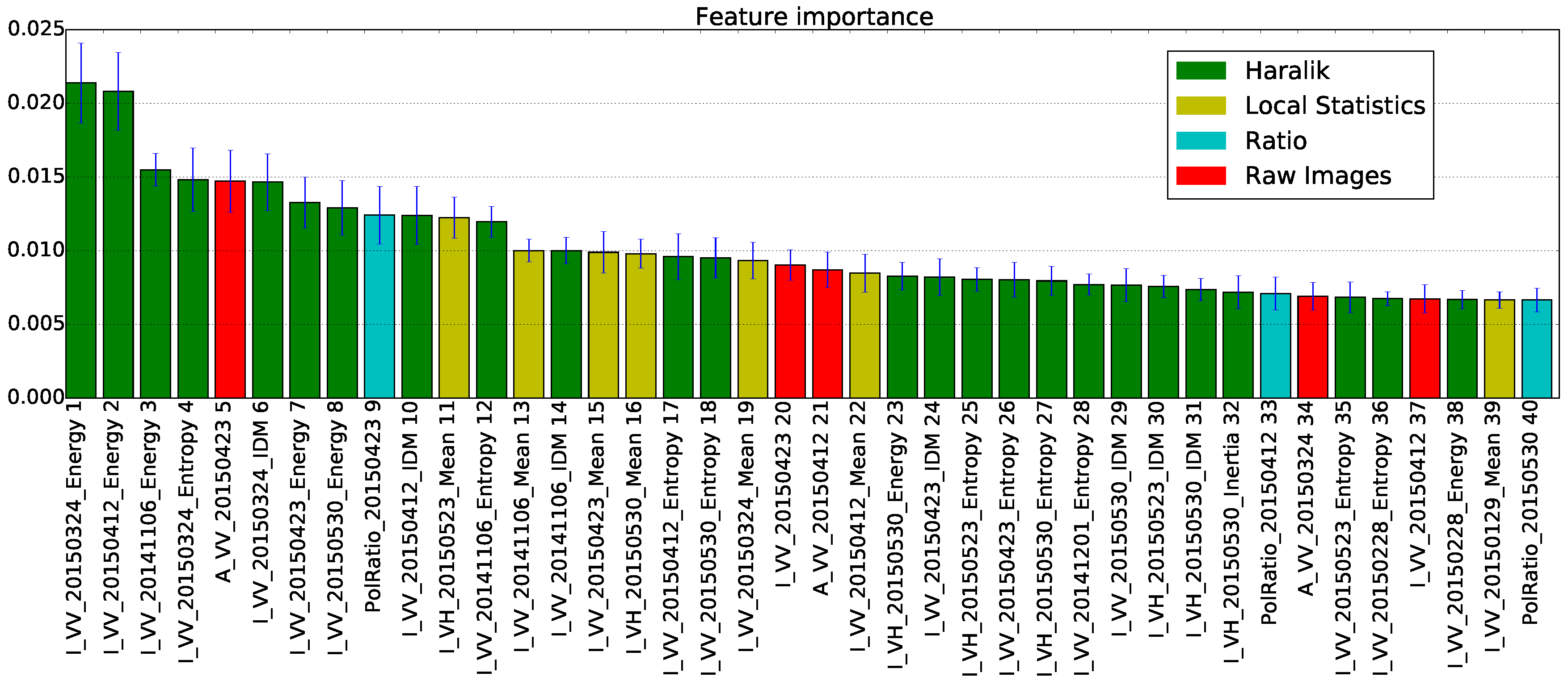
In order to study the most pertinent features for the classification, feature importance is computed for each time point in the time series using all the available images up to the given time point. The incremental classification set up described in Section 3.1 is used.

Figure 3 presents the 40 first features sorted by decreasing importance when the complete time series is used. A color coding is used in order to group features by family (raw images in red, polarimetry ratios in cyan, Haralik textures in green, local statistics in light brown and SFS textures do not appear among the 40 first features). The horizontal axis is labelled with a key containing whether the image was in intensity (I, the modulus square of the complex pixel) or amplitude (A, the square root of I), its polarization (VV or VH), the acquisition date and the name of the texture computed.

It can be seen that local statistics and Haralik textures are the most frequently present and that SFS do not appear among the first 40 features. Among Haralik textures, the most frequent are Energy, Entropy and Inverse Difference Moment. In terms of local statistics, none of the higher moments appear and only the local mean is present. Finally, there seems to be no significant difference between amplitude or intensity for the raw images. In terms of polarimetric information, VV polarization appears as more important and VH polarization has only 8 occurrences over 37. This result may seem surprising. One could have expected that VH polarization, which contains volume scattering information, would be selected as more important than VV polarization. However, features are selected as a complement to the optical ones, and VH polarization and NDVI can be correlated [11]. Three occurrences of the polarimetric ratio are present among the 40 most important features.

In terms of dates, it is not surprising to see that spring dates are the most present, since most of the evolution of the vegetation happens in this period when winter crops are mature and summer crops are just emerging, but this may be correlated with cloud cover. There is also more cloud cover in February, but this is a vegetation dormancy period in the study area. Some occurrences of dates in November appear when soil work for winter crops takes place in the area.

The analysis of feature importance for other time points (using the incremental classification approach) yields the same results in terms of importance for the different families of features.

In the following experiments, the 40 most important SAR features are kept for every classification performed.

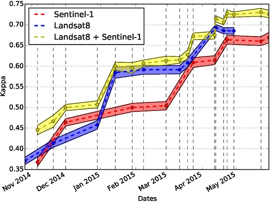
4.2. Impact of SAR Images in the Classification

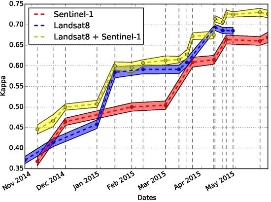
Figure 4 summarizes the accuracy results of the real-time classification simulation for 3 scenarios:

• use of optical imagery alone (blue);
• use of SAR imagery alone (red);
• joint use of optical and SAR imagery (yellow).

The plots show the mean value of κ over 10 random trials together with 95% confidence intervals.

First of all, we observe an expected pattern of increasing accuracy as the season progresses and more data is available. This behavior is the same for the three scenarios. As one can observe, optical data outperforms SAR time series for crop mapping. This is expected, since crop growth is mainly characterized by the time profile of the vegetative activity for which NDVI is a good proxy. There is a short interval in which SAR imagery yields better results during late autumn when ploughing occurs before sowing winter crops. Nevertheless, the red curve shows that SAR image time series alone are able to catch up with optical time series performances at some key dates of the season (April and May).

The joint use of the two types of imagery yields always better results than optical imagery alone (except for one data point in mid April which will be discussed below). Its also remarkable that at the beginning of April, the fusion of the two modalities achieves results which are equivalent to those obtained by the optical imagery alone 1 month later. This an important gain for early crop mapping.

Finally, when the last optical data is available, the gain achieved by the joint use of optical and SAR time series is higher than 0.04 in κ coefficient, with very narrow confidence intervals.

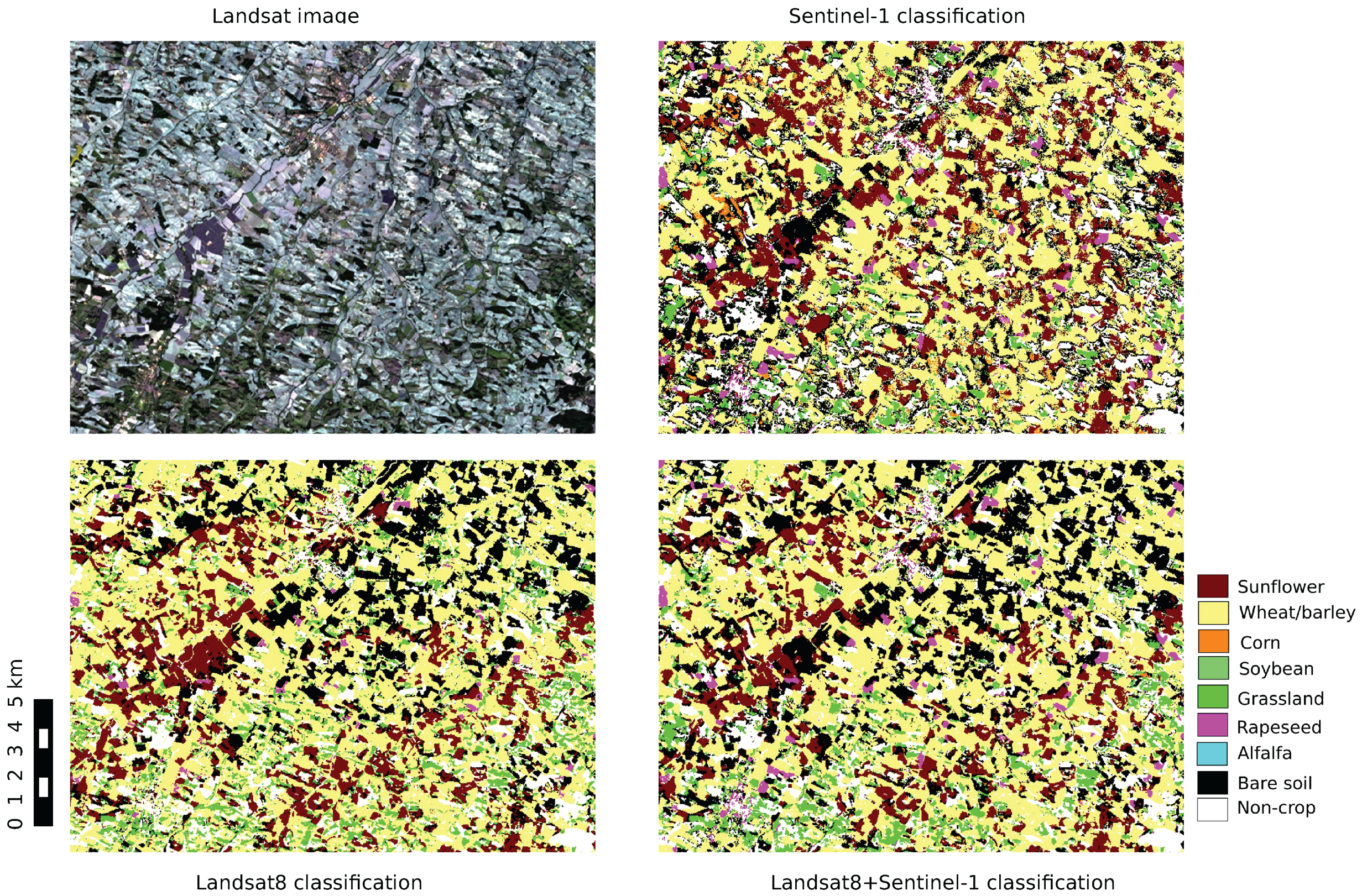
Figure 5 shows an extract of the land cover maps obtained at the end of each time series (Sentinel-1 only, Landsat8 only and both). One can observe that the Sentinel-1 map is noisier than the maps produced using Landsat8 images. Globally, the maps are consistent, but they do not allow a precise interpretation of the differences of behavior between the different configurations.

We analyze in detail the results looking at the confusion matrices. These present the reference class labels in rows and the labels predicted by the classifier in columns. The results are expressed in percentages with respect to the reference labels, and therefore, values in the diagonal represent Producers Accuracy. User Accuracy (UA) values are presented in the bottom row of each matrix. The κ coefficient is given in the legend of each matrix.

Table 6. Confusion matrix for 29-01-2015 using Sentinel-1 alone (3 images). κ = 0.49.

	SF	WB	BS	CO	SO	GR	RA	AL
SF	55.42	20.44	10.72	8.67	0.0	2.21	2.53	0.0
WB	0.73	82.11	12.96	1.13	0.0	1.31	1.76	0.0
BS	4.33	22.2	58.26	4.15	0.0	7.93	3.12	0.0
CO	14.3	12.0	31.79	35.38	0.0	4.89	1.64	0.0
SO	29.58	58.22	0.2	0.0	0.0	0.0	11.99	0.0
GR	0.02	20.34	20.68	1.83	0.0	55.56	1.58	0.0
RA	6.78	22.05	26.57	1.25	0.0	0.14	43.21	0.0
AL	0.07	5.52	8.41	20.95	0.0	65.05	0.0	0.0
UA	57.23	67.63	54.75	54.7	0.0	68.67	60.99	0.0

,

Table 7. Confusion matrix for 29-01-2015 using Landsat8 alone (4 images). κ = 0.58.

	SF	WB	BS	CO	SO	GR	RA	AL
SF	39.25	29.1	18.72	10.9	0.0	1.97	0.07	0.0
WB	0.78	87.02	7.72	1.87	0.0	1.98	0.63	0.0
BS	3.3	19.23	67.35	3.43	0.0	6.01	0.69	0.0
CO	11.03	13.5	16.9	54.24	0.0	4.27	0.06	0.0
SO	26.75	57.82	15.4	0.0	0.0	0.03	0.0	0.0
GR	0.14	16.65	22.28	1.63	0.0	58.97	0.33	0.0
RA	0.59	23.05	8.93	0.33	0.0	3.63	63.47	0.0
AL	0.7	13.24	0.8	29.96	0.0	55.3	0.0	0.0
UA	57.63	69.49	65.79	63.43	0.0	70.83	91.19	0.0

and

Table 8. Confusion matrix for 29-01-2015 using Sentinel-1 (3 images) and Landsat8 (4 images). κ = 0.59.

	SF	WB	BS	CO	SO	GR	RA	AL
SF	47.96	19.88	19.37	10.93	0.0	1.52	0.35	0.0
WB	0.42	86.27	10.17	1.67	0.0	1.24	0.23	0.0
BS	4.16	17.13	68.9	3.54	0.0	5.92	0.34	0.0
CO	12.53	9.75	19.31	56.42	0.0	1.97	0.03	0.0
SO	42.18	53.87	3.95	0.0	0.0	0.0	0.0	0.0
GR	0.02	17.01	20.07	1.59	0.0	61.11	0.2	0.0
RA	1.12	22.39	14.7	2.43	0.0	0.79	58.58	0.0
AL	0.47	3.39	1.63	30.83	0.0	63.68	0.0	0.0
UA	59.26	72.2	63.61	63.39	0.0	76.08	95.0	0.0

show respectively the confusion matrices using Sentinel-1 alone, Landsat8 alone and the two time series together up to 29-01-2015. At this point in time, there is a very small improvement by the use of radar imagery which is mainly concentrated in the better discrimination of sunflower by decreasing the confusion with wheat/barley. Since sunflower is a summer crop, it is not still present, but SAR imagery allows to characterize soil work which precedes the seeding of the summer crops. However, the use of SAR data introduces a low decrease in the accuracy for rapeseed which is confused with bare soil. As expected, soybean and alfalfa are not recognized by any of the classifications. Soybean is predicted as sunflower (another summer crop) or wheat/barley (in the cases where biomass residues from the previous crop are present in the fields). Alfalfa is mostly predicted as grass, which is expected because of the similarity between these two classes.

Table 9. Confusion matrix for 24-03-2015 using Sentinel-1 (5 images). κ = 0.61.

	SF	WB	BS	CO	SO	GR	RA	AL
SF	62.75	3.42	15.34	11.6	0.0	1.52	5.37	0.0
WB	1.26	85.59	9.85	1.03	0.0	1.31	0.95	0.0
BS	4.83	11.8	73.46	3.72	0.0	3.45	2.74	0.0
CO	14.48	1.39	32.67	48.88	0.0	1.35	1.24	0.0
SO	47.79	17.09	34.37	0.07	0.0	0.0	0.69	0.0
GR	0.15	17.03	22.15	1.79	0.0	57.09	1.79	0.0
RA	5.37	6.57	31.35	0.73	0.0	1.31	54.67	0.0
AL	0.0	18.96	15.2	8.41	0.0	57.43	0.0	0.0
UA	58.5	81.92	59.71	62.52	0.0	80.76	68.09	0.0

,

Table 10. Confusion matrix for 24-03-2015 using Landsat8 (7 images). κ = 0.61.

	SF	WB	BS	CO	SO	GR	RA	AL
SF	51.24	26.37	9.02	11.81	0.0	1.43	0.12	0.0
WB	0.97	84.54	9.06	2.8	0.0	2.26	0.37	0.0
BS	2.36	16.0	72.22	4.74	0.0	4.17	0.51	0.0
CO	14.07	7.46	14.05	61.36	0.0	3.02	0.04	0.0
SO	22.85	67.5	9.66	0.0	0.0	0.0	0.0	0.0
GR	0.24	15.74	24.59	2.02	0.0	57.03	0.38	0.0
RA	0.98	24.08	9.56	0.09	0.0	3.63	61.67	0.0
AL	0.0	14.73	0.12	32.57	0.0	52.58	0.0	0.0
UA	63.3	72.06	67.32	60.44	0.0	74.63	93.1	0.0

and

Table 11. Confusion matrix for 24-03-2015 using Sentinel-1 (5 images) and Landsat8 (7 images). κ = 0.67.

	SF	WB	BS	CO	SO	GR	RA	AL
SF	66.84	4.3	15.34	11.78	0.0	1.55	0.2	0.0
WB	1.31	86.32	8.44	2.2	0.0	1.67	0.07	0.0
BS	2.75	10.16	78.41	5.48	0.0	2.99	0.22	0.0
CO	18.0	1.87	16.08	62.4	0.0	1.64	0.01	0.0
SO	41.34	34.73	23.93	0.0	0.0	0.0	0.0	0.0
GR	0.03	14.19	17.79	2.1	0.0	65.75	0.14	0.0
RA	4.41	8.79	22.97	1.86	0.0	2.31	59.67	0.0
AL	0.0	12.1	2.02	17.6	0.0	68.28	0.0	0.0
UA	62.34	83.21	67.83	60.38	0.0	81.82	97.34	0.0

show the confusion matrices for 24-03-2015 using Sentinel-1 alone, Landsat8 alone and both time series together respectively. This date is particularly interesting since the use of SAR data allows a significant increase of κ.

Again, there is an important improvement for sunflower strongly decreasing the confusion with wheat/barley still present in the case of Landsat8. The other noticeable improvement appears on the grass class, which has the same accuracy for each of the two sensors used independently, and its good classification increases about 8% when the two sensors are used together.

It is interesting to note the behavior of the soybean class. While the optical classification makes the same confusions as in the previous studied date, the SAR classification assigns many pixels to the bare soil class. This is due to the fact that, in March, soil work for the summer crops has started. This behavior also appears when the two sensors are used together.

Finally we analyse the confusion matrices for 23-04-2015 (

Table 12. Confusion matrix for 23-04-2015 using Sentinel-1 (7 images). κ = 0.66.

	SF	WB	BS	CO	SO	GR	RA	AL
SF	52.2	4.49	31.02	11.56	0.0	0.22	0.51	0.0
WB	0.53	90.57	5.75	0.5	0.0	1.42	1.23	0.0
BS	5.26	4.86	85.59	2.15	0.0	1.27	0.86	0.0
CO	11.3	2.39	45.0	39.94	0.0	0.87	0.51	0.0
SO	54.51	15.56	29.9	0.03	0.0	0.0	0.0	0.0
GR	0.05	16.14	26.09	1.15	0.0	55.28	1.29	0.0
RA	0.86	6.23	15.38	0.28	0.0	1.29	75.97	0.0
AL	0.0	10.87	29.19	5.85	0.0	54.09	0.0	0.0
UA	60.35	86.79	61.94	65.9	0.0	86.49	85.97	0.0

,

Table 13. Confusion matrix for 23-04-2015 using Landsat8 (9 images). κ = 0.69.

	SF	WB	BS	CO	SO	GR	RA	AL
SF	55.82	10.34	14.44	17.95	0.0	1.25	0.2	0.0
WB	1.05	89.72	4.01	1.94	0.0	2.94	0.35	0.0
BS	2.58	9.75	78.7	4.51	0.0	4.29	0.17	0.0
CO	14.15	5.19	16.18	61.0	0.0	3.39	0.09	0.0
SO	51.44	12.12	35.15	1.29	0.0	0.0	0.0	0.0
GR	0.17	18.45	8.88	1.88	0.0	70.35	0.27	0.0
RA	2.04	19.73	5.79	0.14	0.0	4.34	67.96	0.0
AL	0.22	11.45	0.07	16.65	0.0	71.61	0.0	0.0
UA	63.34	79.17	77.74	60.45	0.0	75.93	95.64	0.0

and

Table 14. Confusion matrix for 23-04-2015 using Sentinel-1 (7 images) and Landsat8 (9 images). κ = 0.73.

	SF	WB	BS	CO	SO	GR	RA	AL
SF	58.33	8.64	14.28	17.62	0.0	0.89	0.24	0.0
WB	0.53	92.39	3.42	1.34	0.0	2.08	0.24	0.0
BS	2.33	7.6	82.61	4.65	0.0	2.53	0.28	0.0
CO	13.9	3.83	16.76	62.42	0.0	3.04	0.04	0.0
SO	48.83	15.66	35.02	0.5	0.0	0.0	0.0	0.0
GR	0.01	17.47	10.97	1.45	0.0	69.49	0.61	0.0
RA	1.46	9.44	8.06	0.24	0.0	3.17	77.63	0.0
AL	0.0	7.09	0.18	14.94	0.0	77.79	0.0	0.0
UA	67.4	83.3	77.72	62.68	0.0	81.24	95.58	0.0

for Sentinel-1, Landsat8 and both sensors together respectively). For this case, we observe a degradation of the accuracy in sunflower with respect to the previous period, which is mainly due to an increasing confusion in the SAR case with bare soil, since at this point in time sunflower has emerged in some fields and not in others. There is also a decrease in the Landsat8 case, where the confusion with corn increases (both are summer crops starting to emerge at this point in time).

The increase in κ observed for this date in Figure 4 are distributed among all the classes and it is difficult to point out a particular class.

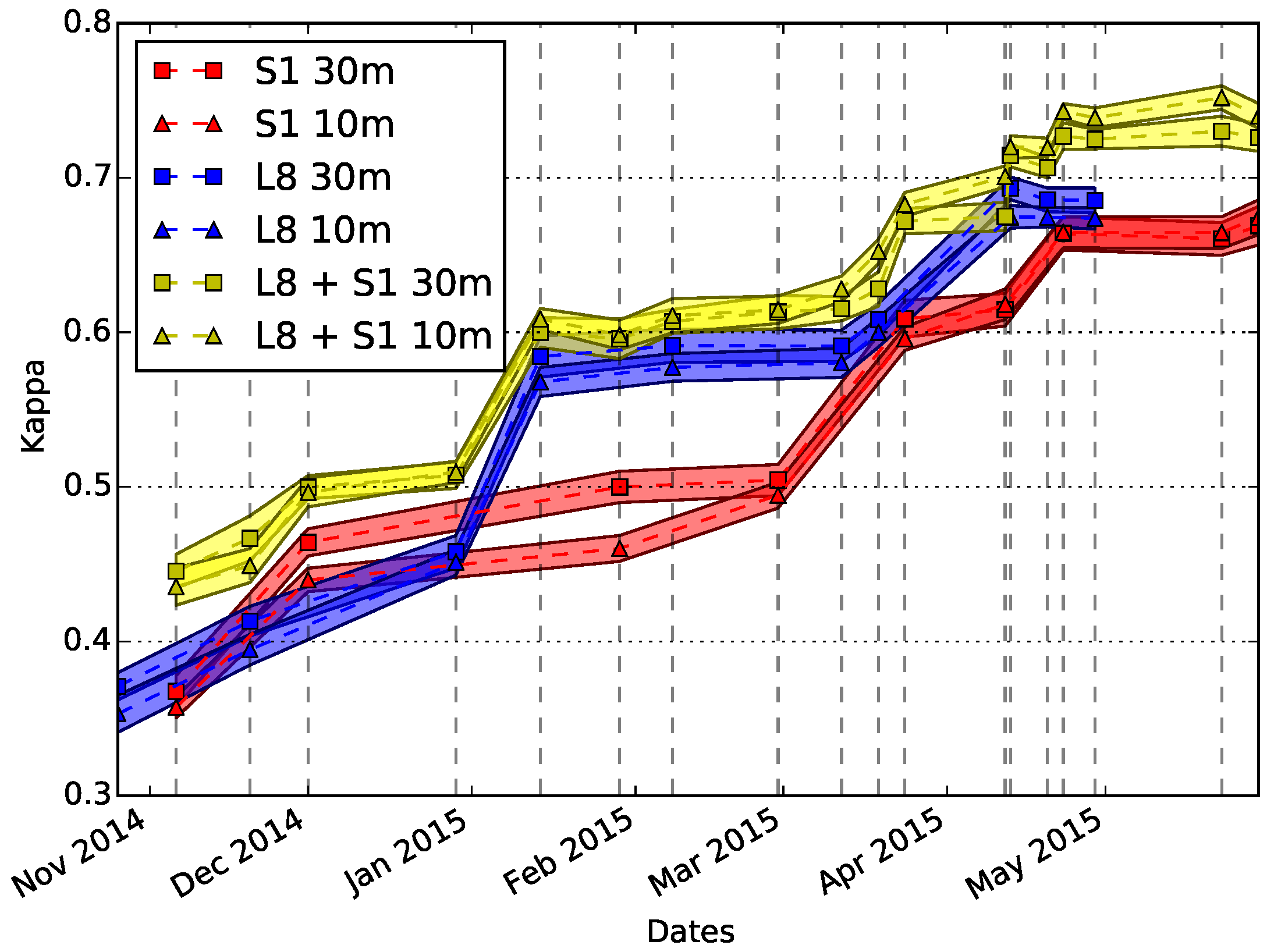
4.3. Impact of Image Resolution and Speckle Filtering

In this section, the influence of the spatial resolution (30 m or 10 m) is investigated. Figure 6 compares the two resolution scenarios: SAR imagery resampled to the Landsat8 pixel size, and optical imagery resampled to the Sentinel-1 10 m pixel size. We see that there is no significant difference from a statistical point of view (overlapping confidence intervals) between the two resolutions, except for the winter period in the case where only SAR data is used. In this case, the 30 m resolution seems more appropriate, probably due to the despeckling effect of the averaging performed by the resampling at 30 m This result can be explained by the field size in the study area which, as Table 1, is larger than 2 ha for most of the classes.

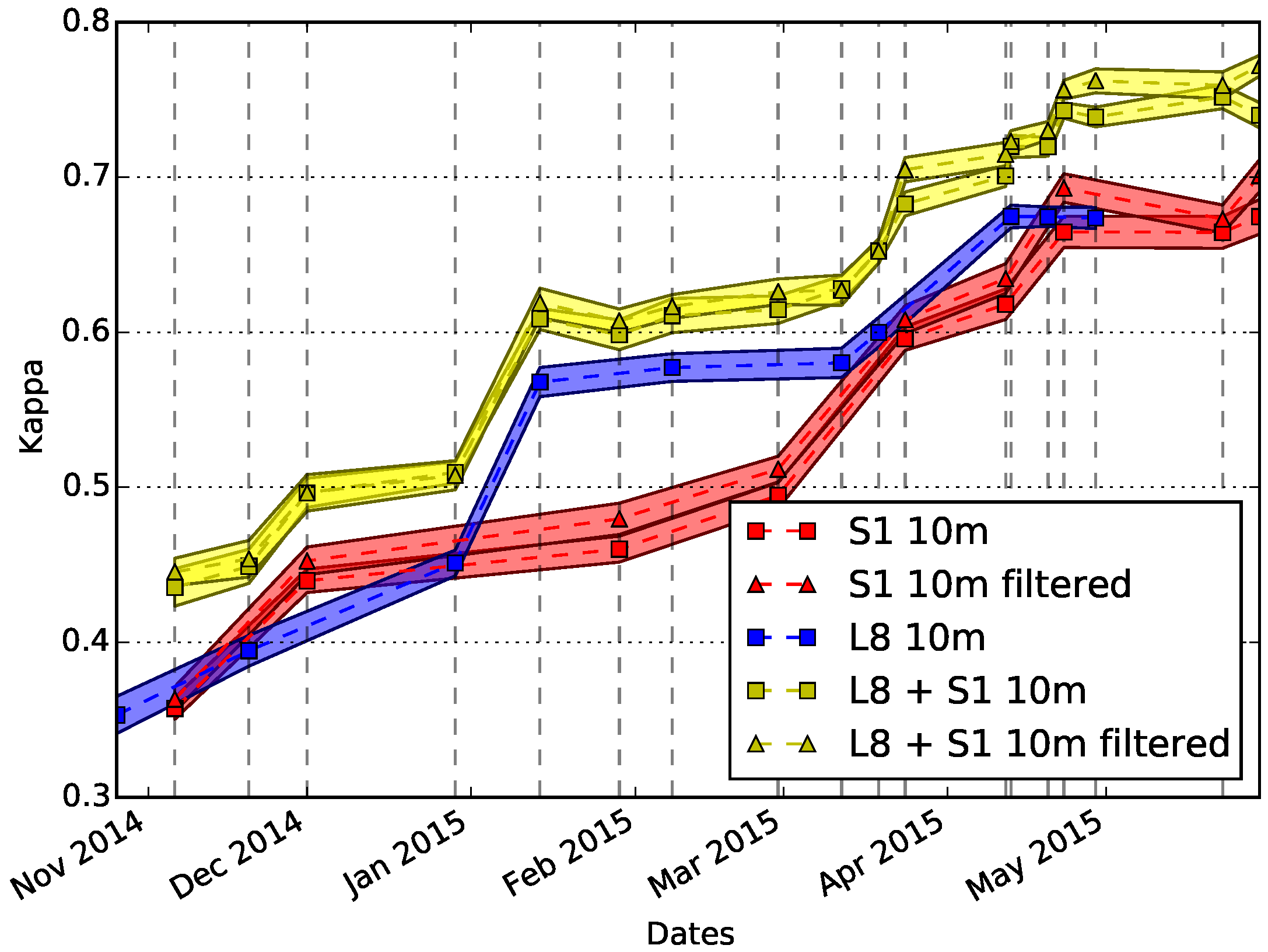
Figure 7 shows the classification accuracy for the data resampled to 10 m and shows the influence of speckle filtering. One can observe that, when SAR and optical data are used together, the speckle filtering introduces a statistically significant small improvement towards the end of the season.

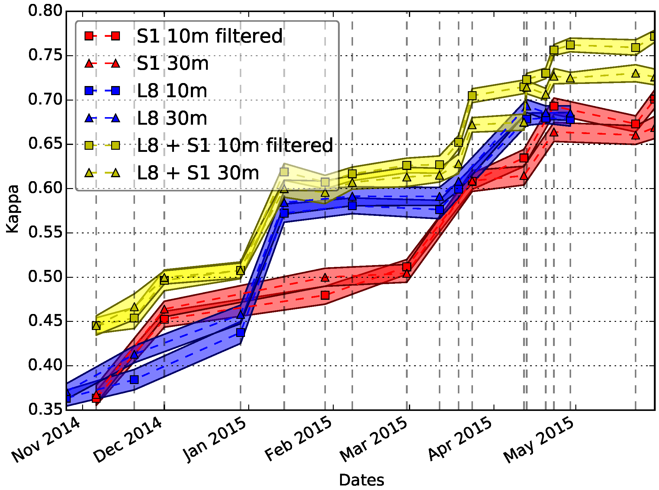
Resampling all the data to a 10 m grid involves high computational times due to the resampling itself, but also to the larger volumes of data to be processed. Figure 8 shows the plots of classification accuracy for the case of data at 10 m and speckle filtering and data at 30 m without speckle filtering. Better performances are obtained by working at the finer resolution and using the speckle filtering. As in the previous case, the improvement is observed even in the case where optical and SAR data are jointly used. The largest improvement is observed at the end of the season.

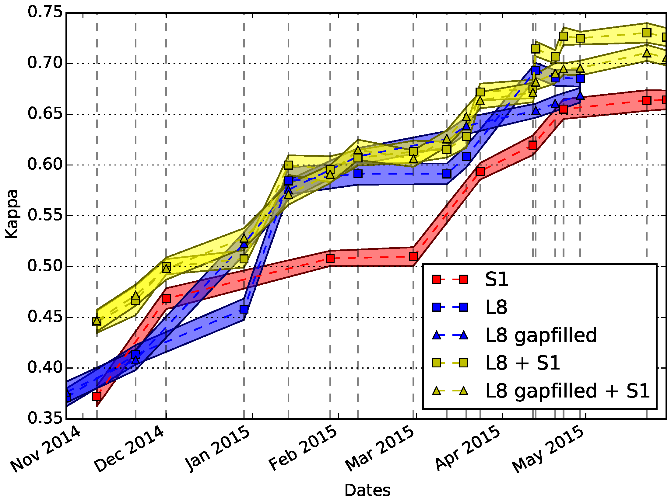
4.4. Impact of Gap-Filling

This section presents the evaluation of the gap-filling applied to the optical SITS to clean cloudy pixels as described in Section 3.4.

Figure 9 summarizes the results of the experiment. First of all, it is interesting to note that for the optical data alone, the gap-filled time series yields better results than the series without gap-filling until the image acquired on April 13th. An investigation in the data set showed that errors in the cloud screening procedure masked a large extent of the reference data for this date and missed some clouds in the following dates producing incorrect interpolated values, which strongly affected the quality of the classifier. The trend of the curves for the optical data indicate that this error may be compensated by the additional images acquired later. However, this kind of error can have an important impact in the classification. Before this date, one can observe that gap-filled optical data yields performances statistically equivalent to those of the joint use of optical and SAR data. Nevertheless, at the beginning of the season, using the two time series together has still a positive impact on the crop type identification. In the case of the joint use of the two time series, one can observe that the gap-filling does not bring any improvement even for the periods on which the gap-filling was useful for the optical data alone. After the dates where the gap-filling artifact is present, as in the optical SITS alone, the non gap-filled case allows to achieve better performances.

Therefore, we can conclude that the joint use of SAR and optical time series does not benefit from a temporal gap-filling processing. This simplifies the processing chain and reduces the computational cost, which is a key element of an operational land cover map production system.

5. Conclusions

In this paper, the impact of high temporal resolution SAR satellite image time series (SITS) as a complement to high temporal and spatial resolution optical imagery for early crop type mapping has been studied.

Sentinel-1 SAR image time series were used with Landsat8 SITS showing that a significant improvement in classification accuracy can be achieved allowing to obtain land cover mapping earlier in the season with respect to the case where optical imagery is used alone.

The most pertinent features derived from SAR imagery where analyzed, showing that Haralik textures (Entropy, Inertia), the polarization ratio and the local mean together with the VV imagery contain most of the information needed for an accurate classification.

The influence of image resolution and speckle filtering where also investigated, leading to the conclusion that working at 10 m resolution and using speckle filtering improves the results.

Finally, the effect of temporal gap-filling of the optical SITS was investigated, revealing that errors in the cloud screening procedure can have high impact in the classification accuracy if they coincide with ground reference data used for the classifier training. The use of SAR imagery allows to use optical data without gap-filling yielding results which are equivalent to the use of gap-filling in the case of perfect cloud screening, and better results in the case of cloud screening errors.

These results are relevant for the upcoming availability of Sentinel-1 and Sentinel-2 dense image time series which will provide respectively a 6-day and 5-day revisit cycle during their full capacity operational phase.

References

1. Foley, J.A.; Ramankutty, N.; Brauman, K.A.; Cassidy, E.S.; Gerber, J.S.; Johnston, M.; Mueller, N.D.; O’Connell, C.; Ray, D.K.; West, P.C.; et al. Solutions for a cultivated planet. Nature 2011, 478, 337–342. [Google Scholar] [CrossRef] [PubMed]
2. Godfray, H.C.J.; Beddington, J.R.; Crute, I.R.; Haddad, L.; Lawrence, D.; Muir, J.F.; Pretty, J.; Robinson, S.; Thomas, S.M.; Toulmin, C. Food security: The challenge of feeding 9 billion people. Science 2010, 327, 812–818. [Google Scholar] [CrossRef] [PubMed]
3. Rounsevell, M.; Ewert, F.; Reginster, I.; Leemans, R.; Carter, T. Future scenarios of European agricultural land use: II. Projecting changes in cropland and grassland. Agric. Ecosyst. Environ. 2005, 107, 117–135. [Google Scholar] [CrossRef]
4. Searchinger, T.; Heimlich, R.; Houghton, R.A.; Dong, F.; Elobeid, A.; Fabiosa, J.; Tokgoz, S.; Hayes, D.; Yu, T.H. Use of U.S. croplands for biofuels increases greenhouse gases through emissions from land-use change. Science 2008, 319, 1238–1240. [Google Scholar] [CrossRef] [PubMed]
5. Green, R.E.; Cornell, S.J.; Scharlemann, J.P.W.; Balmford, A. Farming and the fate of wild nature. Science 2005, 307, 550–555. [Google Scholar] [CrossRef] [PubMed]
6. Tilman, D. Forecasting agriculturally driven global environmental change. Science 2001, 292, 281–284. [Google Scholar] [CrossRef] [PubMed]
7. Torres, R.; Snoeij, P.; Geudtner, D.; Bibby, D.; Davidson, M.; Attema, E.; Potin, P.; Rommen, B.; Floury, N.; Brown, M.; et al. GMES Sentinel-1 mission. Remote Sens. Environ. 2012, 120, 9–24. [Google Scholar] [CrossRef]
8. Drusch, M.; Bello, U.D.; Carlier, S.; Colin, O.; Fernandez, V.; Gascon, F.; Hoersch, B.; Isola, C.; Laberinti, P.; Martimort, P.; et al. Sentinel-2: ESA’s optical high-resolution mission for GMES operational services. Remote Sens. Environ. 2012, 120, 25–36. [Google Scholar] [CrossRef]
9. Inglada, J.; Arias, M.; Tardy, B.; Hagolle, O.; Valero, S.; Morin, D.; Dedieu, G.; Sepulcre, G.; Bontemps, S.; Defourny, P.; et al. Assessment of an operational system for crop type map production using high temporal and spatial resolution satellite optical imagery. Remote Sens. 2015, 7, 12356–12379. [Google Scholar] [CrossRef]
10. Skriver, H.; Svendsen, M.; Thomsen, A. Multitemporal C-and L-band polarimetric signatures of crops. IEEE Trans. Geosci. Remote Sens. 1999, 37, 2413–2429. [Google Scholar] [CrossRef]
11. Schotten, C.G.J.; Rooy, W.W.L.V.; Janssen, L.L.F. Assessment of the capabilities of multi-temporal ERS-1 SAR data to discriminate between agricultural crops. Int. J. Remote Sens. 1995, 16, 2619–2637. [Google Scholar] [CrossRef]
12. Balzter, H.; Cole, B.; Thiel, C.; Schmullius, C. Mapping CORINE land cover from Sentinel-1a SAR and SRTM digital elevation model data using random forests. Remote Sens. 2015, 7, 14876–14898. [Google Scholar] [CrossRef]
13. Skriver, H. Crop classification by multitemporal C-and L-band single-and dual-polarization and fully polarimetric SAR. IEEE Trans. Geosci. Remote Sens. 2012, 50, 2138–2149. [Google Scholar] [CrossRef]
14. Moran, M.S.; Alonso, L.; Moreno, J.F.; Mateo, M.P.C.; de la Cruz, D.F.; Montoro, A. A RADARSAT-2 quad-polarized time series for monitoring crop and soil conditions in Barrax, Spain. IEEE Trans. Geosci. Remote Sens. 2012, 50, 1057–1070. [Google Scholar] [CrossRef]
15. Skriver, H.; Mattia, F.; Satalino, G.; Balenzano, A.; Pauwels, V.R.N.; Verhoest, N.E.C.; Davidson, M. Crop classification using short-revisit multitemporal SAR data. IEEE J. Sel. Top. Appl. Earth Observ. Remote Sens. 2011, 4, 423–431. [Google Scholar] [CrossRef]
16. McNairn, H.; Kross, A.; Lapen, D.; Caves, R.; Shang, J. Early season monitoring of corn and soybeans with TerraSAR-X and RADARSAT-2. Int. J. Appl. Earth Observ. Geoinf. 2014, 28, 252–259. [Google Scholar] [CrossRef]
17. Zhang, J. Multi-source remote sensing data fusion: Status and trends. Int. J. Image Data Fusion 2010, 1, 5–24. [Google Scholar] [CrossRef]
18. McNairn, H.; Champagne, C.; Shang, J.; Holmstrom, D.; Reichert, G. Integration of optical and Synthetic Aperture Radar (SAR) imagery for delivering operational annual crop inventories. ISPRS J. Photogramm. Remote Sens. 2009, 64, 434–449. [Google Scholar] [CrossRef]
19. Zhu, L.; Tateishi, R. Fusion of multisensor multitemporal satellite data for land cover mapping. Int. J. Remote Sens. 2006, 27, 903–918. [Google Scholar] [CrossRef]
20. Blaes, X.; Vanhalle, L.; Defourny, P. Efficiency of crop identification based on optical and SAR image time series. Remote Sens. Environ. 2005, 96, 352–365. [Google Scholar] [CrossRef]
21. Hegarat-Mascle, S.L.; Quesney, A.; Vidal-Madjar, D.; Taconet, O.; Normand, M.; Loumagne, C. Land cover discrimination from multitemporal ERS images and multispectral Landsat images: A study case in an agricultural area in France. Int. J. Remote Sens. 2000, 21, 435–456. [Google Scholar] [CrossRef]
22. Chust, G.; Ducrot, D.; Pretus, J.L. Land cover discrimination potential of radar multitemporal series and optical multispectral images in a Mediterranean cultural landscape. Int. J. Remote Sens. 2004, 25, 3513–3528. [Google Scholar] [CrossRef]
23. Forkuor, G.; Conrad, C.; Thiel, M.; Ullmann, T.; Zoungrana, E. Integration of optical and Synthetic Aperture Radar imagery for improving crop mapping in Northwestern Benin, West Africa. Remote Sens. 2014, 6, 6472–6499. [Google Scholar] [CrossRef]
24. Skakun, S.; Kussul, N.; Shelestov, A.Y.; Lavreniuk, M.; Kussul, O. Efficiency assessment of multitemporal C-band Radarsat-2 intensity and Landsat-8 surface reflectance satellite imagery for crop classification in Ukraine. IEEE J. Sel. Top. Appl Earth Observ. Remote Sens. 2015. [Google Scholar] [CrossRef]
25. Villa, P.; Stroppiana, D.; Fontanelli, G.; Azar, R.; Brivio, P. In-Season Mapping of Crop Type with Optical and X-Band SAR Data: A Classification Tree Approach Using Synoptic Seasonal Features. Remote Sens. 2015, 7, 12859–12886. [Google Scholar] [CrossRef]
26. Reiche, J.; Verbesselt, J.; Hoekman, D.; Herold, M. Fusing Landsat and SAR time series to detect deforestation in the tropics. Remote Sens. Environ. 2015, 156, 276–293. [Google Scholar] [CrossRef]
27. Lehmann, E.A.; Caccetta, P.; Lowell, K.; Mitchell, A.; Zhou, Z.S.; Held, A.; Milne, T.; Tapley, I. SAR and optical remote sensing: Assessment of complementarity and interoperability in the context of a large-scale operational forest monitoring system. Remote Sens. Environ. 2015, 156, 335–348. [Google Scholar] [CrossRef]
28. Reiche, J.; de Bruin, S.; Hoekman, D.; Verbesselt, J.; Herold, M. A Bayesian approach to combine Landsat and ALOS PALSAR time series for near real-time deforestation detection. Remote Sens. 2015, 7, 4973–4996. [Google Scholar] [CrossRef]
29. Lehmann, E.A.; Caccetta, P.A.; Zhou, Z.S.; McNeill, S.J.; Wu, X.; Mitchell, A.L. Joint processing of Landsat and ALOS-PALSAR data for forest mapping and monitoring. IEEE Trans. Geosci. Remote Sens. 2012, 50, 55–67. [Google Scholar] [CrossRef]
30. Laurin, G.V.; Liesenberg, V.; Chen, Q.; Guerriero, L.; Frate, F.D.; Bartolini, A.; Coomes, D.; Wilebore, B.; Lindsell, J.; Valentini, R. Optical and SAR sensor synergies for forest and land cover mapping in a tropical site in West Africa. Int. J. Appl. Earth Observ. Geoinf. 2013, 21, 7–16. [Google Scholar] [CrossRef]
31. Schuster, C.; Schmidt, T.; Conrad, C.; Kleinschmit, B.; Förster, M. Grassland habitat mapping by intra-annual time series analysis–Comparison of RapidEye and TerraSAR-X satellite data. Int. J. Appl. Earth Observ. Geoinf. 2015, 34, 25–34. [Google Scholar] [CrossRef]
32. Osman, J.; Inglada, J.; Dejoux, J.F. Assessment of a Markov logic model of crop rotations for early crop mapping. Comput. Electron. Agric. 2015, 113, 234–243. [Google Scholar] [CrossRef] [Green Version]
33. Valero, S.; Morin, D.; Inglada, J.; Sepulcre, G.; Arias, M.; Hagolle, O.; Dedieu, G.; Bontemps, S.; Defourny, P.; Koetz, B. Production of a dynamic cropland mask by processing remote sensing image series at high temporal and spatial resolutions. Remote Sens. 2016, 8, 55. [Google Scholar] [CrossRef]
34. Irons, J.R.; Dwyer, J.L.; Barsi, J.A. The next Landsat satellite: The Landsat data continuity mission. Remote Sens. Environ. 2012, 122, 11–21. [Google Scholar] [CrossRef]
35. Hagolle, O.; Sylvander, S.; Huc, M.; Claverie, M.; Clesse, D.; Dechoz, C.; Lonjou, V.; Poulain, V. SPOT4 (Take5): Simulation of Sentinel-2 time series on 45 large sites. Remote Sens. 2015, 7, 12242–12264. [Google Scholar] [CrossRef]
36. Sentinel-1 Team. Sentinel-1 User Handbook; European Space Agency: Rome, Italy, 2013. [Google Scholar]
37. The Sentinel-1 Toolbox. Available online: https://sentinel.esa.int/web/sentinel/toolboxes/sentinel-1 (accessed on 8 December 2015).
38. Congalton, R.G. A review of assessing the accuracy of classifications of remotely sensed data. Remote Sens. Environ. 1991, 37, 35–46. [Google Scholar] [CrossRef]
39. Michel, J.; Grizonnet, M. State of the Orfeo Toolbox. In Proceedings of the 2015 IEEE International Geoscience and Remote Sensing Symposium (IGARSS), Milan, Italy, 26–31 July 2015; pp. 1336–1339.
40. Burges, C.J. A tutorial on support vector machines for pattern recognition. Data Min. Knowl. Discov. 1998, 2, 121–167. [Google Scholar] [CrossRef]
41. Rodriguez-Galiano, V.; Ghimire, B.; Rogan, J.; Chica-Olmo, M.; Rigol-Sanchez, J. An assessment of the effectiveness of a random forest classifier for land-cover classification. ISPRS J. Photogramm. Remote Sens. 2012, 67, 93–104. [Google Scholar] [CrossRef]
42. Tso, B.; Mather, P.M. Crop discrimination using multi-temporal SAR imagery. Int. J. Remote Sens. 1999, 20, 2443–2460. [Google Scholar] [CrossRef]
43. Haralik, R. Statistical and structured approaches to the description of textures. TIIRE 1979, 5, 98–118. [Google Scholar]
44. Huang, X.; Zhang, L.; Li, P. Classification and extraction of spatial features in urban areas using high-resolution multispectral imagery. IEEE Geosci. Remote Sens. Lett. 2007, 4, 260–264. [Google Scholar] [CrossRef]
45. Tucker, C.J. Red and photographic infrared linear combinations for monitoring vegetation. Remote Sens. Environ. 1979, 8, 127–150. [Google Scholar] [CrossRef]
46. McFeeters, S. The use of the Normalized Difference Water Index (NDWI) in the delineation of open water features. Int. J. Remote Sens. 1996, 17, 1425–1432. [Google Scholar] [CrossRef]
47. Breiman, L. Random forests. Mach. Learn. 2001, 45, 5–32. [Google Scholar] [CrossRef]
48. Genuer, R.; Poggi, J.M.; Tuleau-Malot, C. Variable selection using random forests. Pattern Recognit. Lett. 2010, 31, 2225–2236. [Google Scholar] [CrossRef]
49. Strobl, C.; Boulesteix, A.L.; Zeileis, A.; Hothorn, T. Bias in random forest variable importance measures: Illustrations, sources and a solution. BMC Bioinf. 2007, 8, 25. [Google Scholar] [CrossRef] [PubMed] [Green Version]
50. Strobl, C.; Boulesteix, A.L.; Kneib, T.; Augustin, T.; Zeileis, A. Conditional variable importance for random forests. BMC Bioinf. 2008, 9, 307. [Google Scholar] [CrossRef] [PubMed] [Green Version]
51. Pedregosa, F.; Varoquaux, G.; Gramfort, A.; Michel, V.; Thirion, B.; Grisel, O.; Blondel, M.; Prettenhofer, P.; Weiss, R.; Dubourg, V.; et al. Scikit-learn: Machine learning in Python. J. Mach. Learn. Res. 2011, 12, 2825–2830. [Google Scholar]
52. Guyon, I.; Weston, J.; Barnhill, S.; Vapnik, V. Gene selection for cancer classification using support vector machines. Mach. Learn. 2002, 46, 389–422. [Google Scholar] [CrossRef]
53. Inglada, J.; Mercier, G. A new statistical similarity measure for change detection in multitemporal SAR images and its extension to multiscale change analysis. IEEE Trans. Geosci. Remote Sens. 2007, 45, 1432–1445. [Google Scholar] [CrossRef]
54. Lee, J.S. Speckle suppression and analysis for synthetic aperture radar images. Opt. Eng. 1986, 25, 255636. [Google Scholar] [CrossRef]
55. Fjortoft, R.; Delignon, Y.; Pieczynski, W.; Sigelle, M.; Tupin, F. Unsupervised classification of radar images using hidden Markov chains and hidden Markov random fields. IEEE Trans. Geosci. Remote Sens. 2003, 41, 675–686. [Google Scholar] [CrossRef]
56. Melgani, F.; Serpico, S. A Markov random field approach to spatio-temporal contextual image classification. IEEE Trans. Geosci. Remote Sens. 2003, 41, 2478–2487. [Google Scholar] [CrossRef]
57. Tison, C.; Nicolas, J.M.; Tupin, F.; Maitre, H. A new statistical model for Markovian classification of urban areas in high-resolution SAR images. IEEE Trans. Geosci. Remote Sens. 2004, 42, 2046–2057. [Google Scholar] [CrossRef]
Figure 1. Study site located in the south-west of France. Field survey data is displayed in yellow on top of a Landsat8 image.
Remotesensing 08 00362 g001
Figure 2. Kappa coefficient of the classification using both Landsat8 and Sentinel-1 images as a function of the number of SAR features sorted by importance. The results with Landsat8 data alone are plotted as a baseline. Line width indicates 95% confidence intervals.
Remotesensing 08 00362 g002
Figure 3. 40 first features sorted by importance. Error bars indicate 95% confidence intervals.
Remotesensing 08 00362 g003
Figure 4. Kappa coefficient of the real-time classification simulation for 3 scenarios with 95% confidence intervals.
Remotesensing 08 00362 g004
Figure 5. Land-cover maps at the end of the time series (extract). Landsat8 image (upper left), Sentinel-1 map (upper right), Landsat8 map (lower left), Sentinel-1 and Landsat8 map (lower right).
Remotesensing 08 00362 g005
Figure 6. Comparison of classification accuracy between data resampled to 30 m and data resampled to 10 m.
Remotesensing 08 00362 g006
Figure 7. Comparison of classification accuracy with data resampled to 10 m with and without speckle filtering.
Remotesensing 08 00362 g007
Figure 8. Comparison of classification accuracy with data resampled to 10 m with speckle filtering and data at 30 m without speckle filtering.
Remotesensing 08 00362 g008
Figure 9. Analysis of the influence of the use of temporal gap-filling in the optical time series
Remotesensing 08 00362 g009