
A Combined Satellite-Derived Drought Indicator to Support Humanitarian Aid Organizations

 , ,
, ,  ,
,  ,
,
Abstract
:
1. Introduction
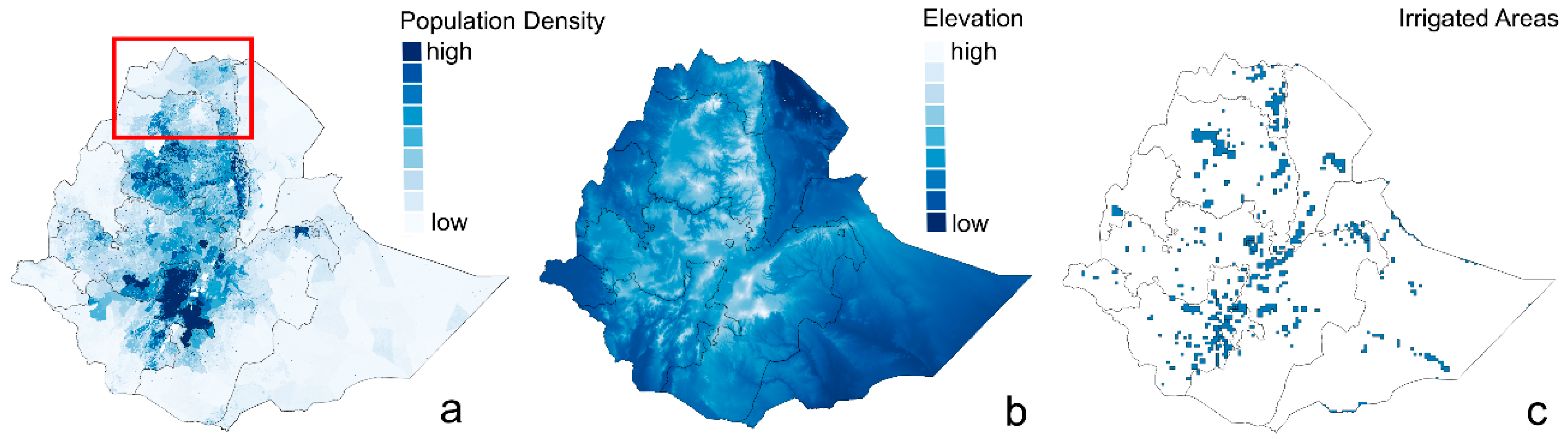
2. Study Area
3. Data and Methods
3.1. Satellite Data and Drought Indices
3.1.1. Satellite-Derived Soil Moisture
3.1.2. Advanced NDVI Products
3.1.3. Benchmark Drought Indices
- the self-calibrated Palmer Drought Severity Index (scPDSI); and
- the Standardized Precipitation Evapotranspiration Index (SPEI).
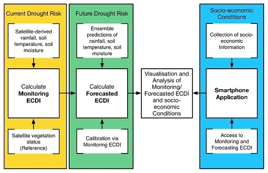
3.2. Methods
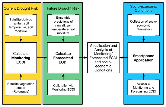
3.2.1. Computation of the Monitoring ECDI
- PDI is the Precipitation Drought Index (an individual index is calculated for precipitation, land surface temperature and soil moisture)
- P* is the decadal precipitation average
- RL*(P*) maximum number of successive decades below long term average rainfall in the interest period (run-length)
- IP interest period (longer IPs detect more severe drought events)
- RL* is the Run Length parameter
- n number of years with data
- j summation running parameter covering the interest period (IP)
- k summation running parameter covering the years where data are available
- d time unit (decade or month)
- y year
- PDI is the Precipitation Drought Index
- IP interest period
- T* is modified Temperature
- P* is modified precipitation
- RL* is modified run length
- PDIscaled is the new scaled value
- PDImin is the minimum value of the decade compared to all decades available
- PDImax is the maximum value of the decades compared to all decades available
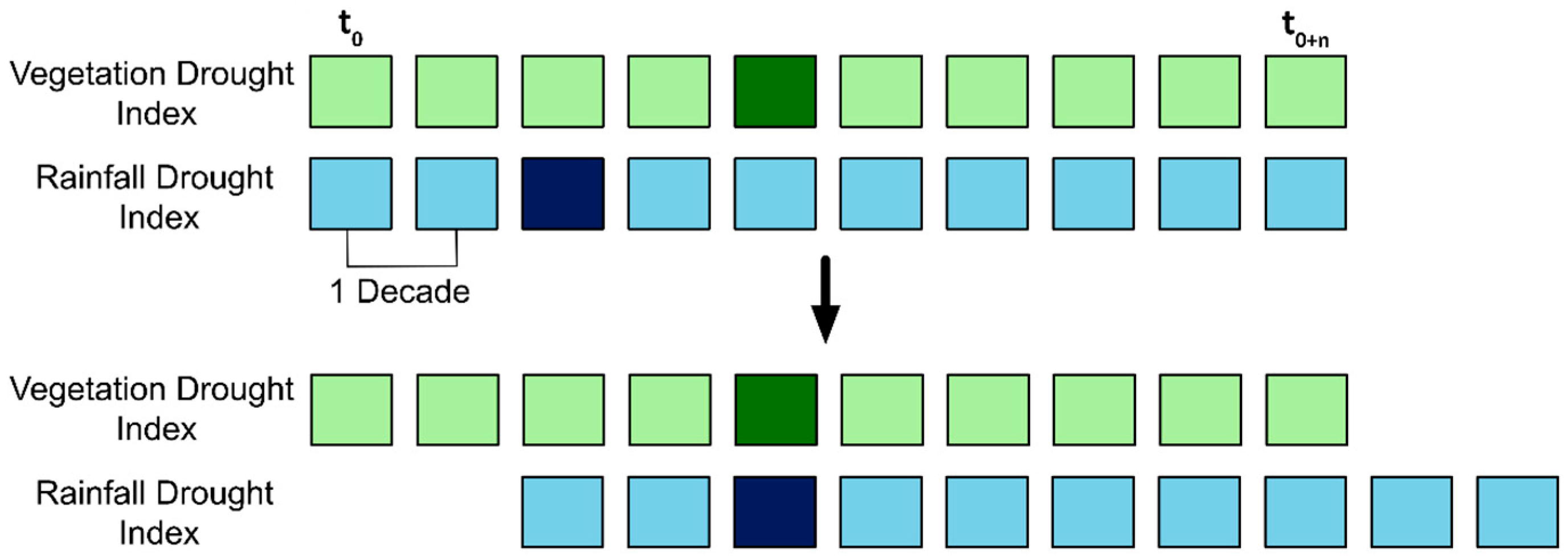
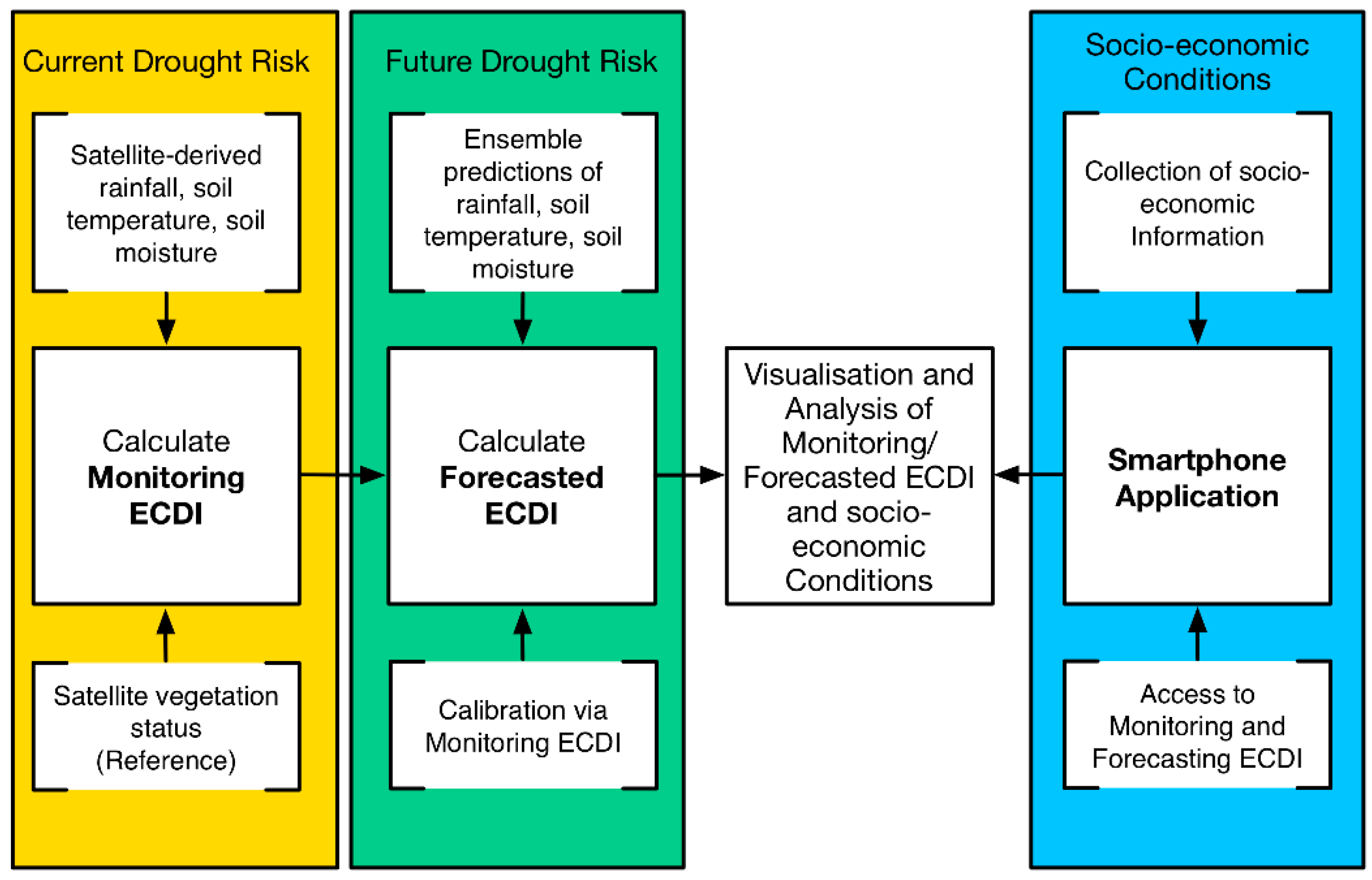
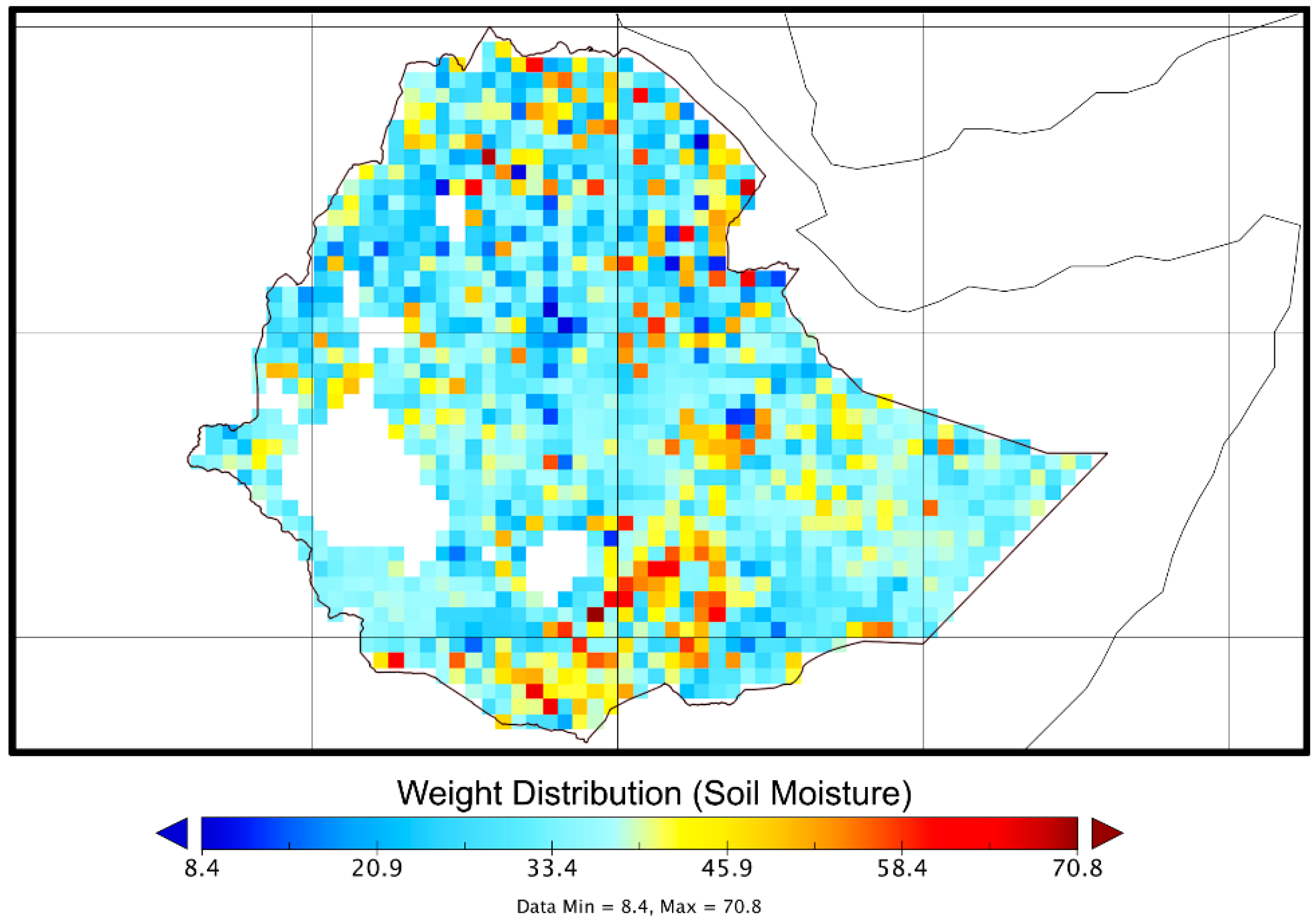
3.2.2. Adjustment of Weights
- ECDI Enhanced Combined Drought Index
- w Weight for each individual drought index (e.g., rainfall)
- DI Individual drought index
- n number of drought indices used to calculate the CDI
- i running parameter covering the number of drought indices
- w weight for the respective drought index
- lag* modified time lag for the respective parameter
- corr* modified correlation coefficient for the respective parameter
- i index for the respective parameter/drought index
- j running parameter covering all parameters used for the ECDI calculation
- n number of individual drought indices used for the ECDI calculation
3.2.3. Drought Risk Warning Levels
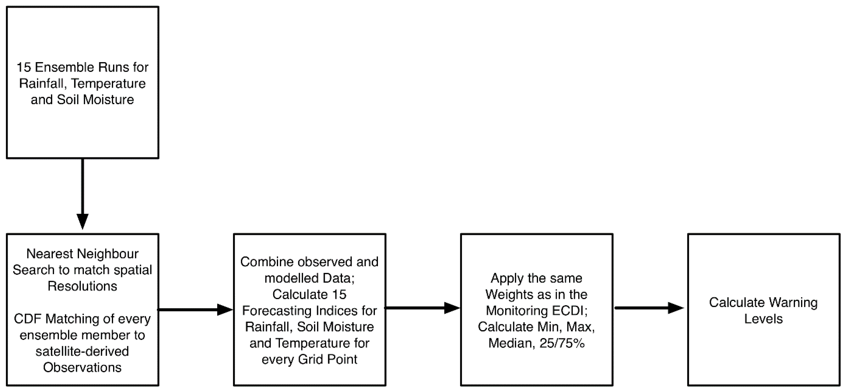
3.2.4. Computation of the Forecasted ECDI
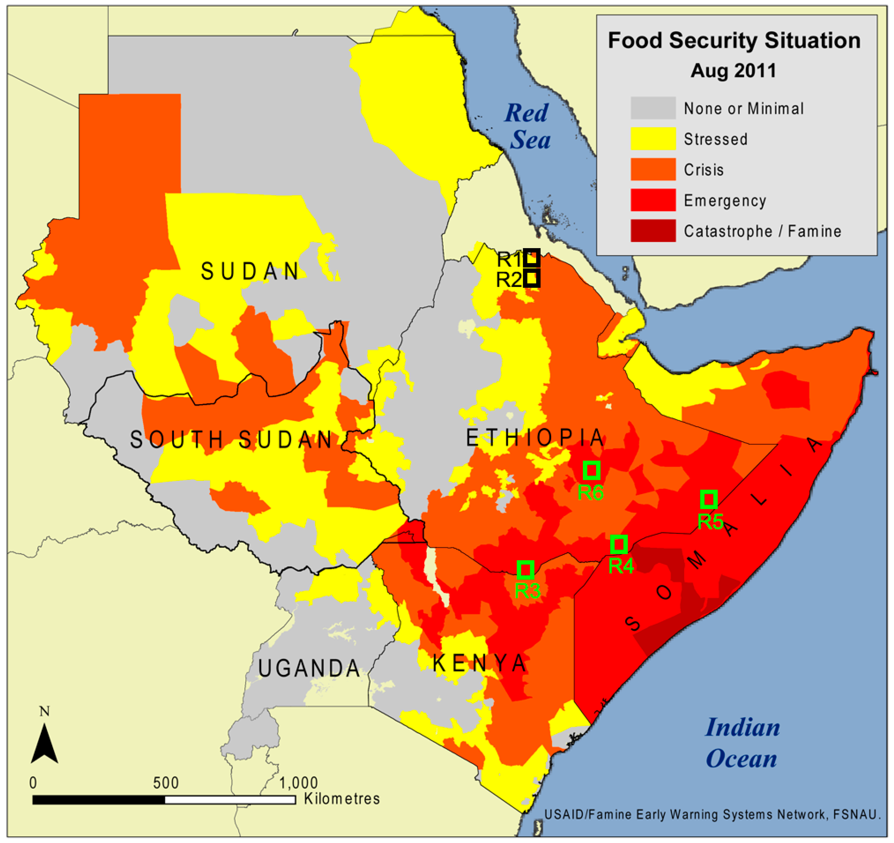
3.3. Comparison and Validation
- -
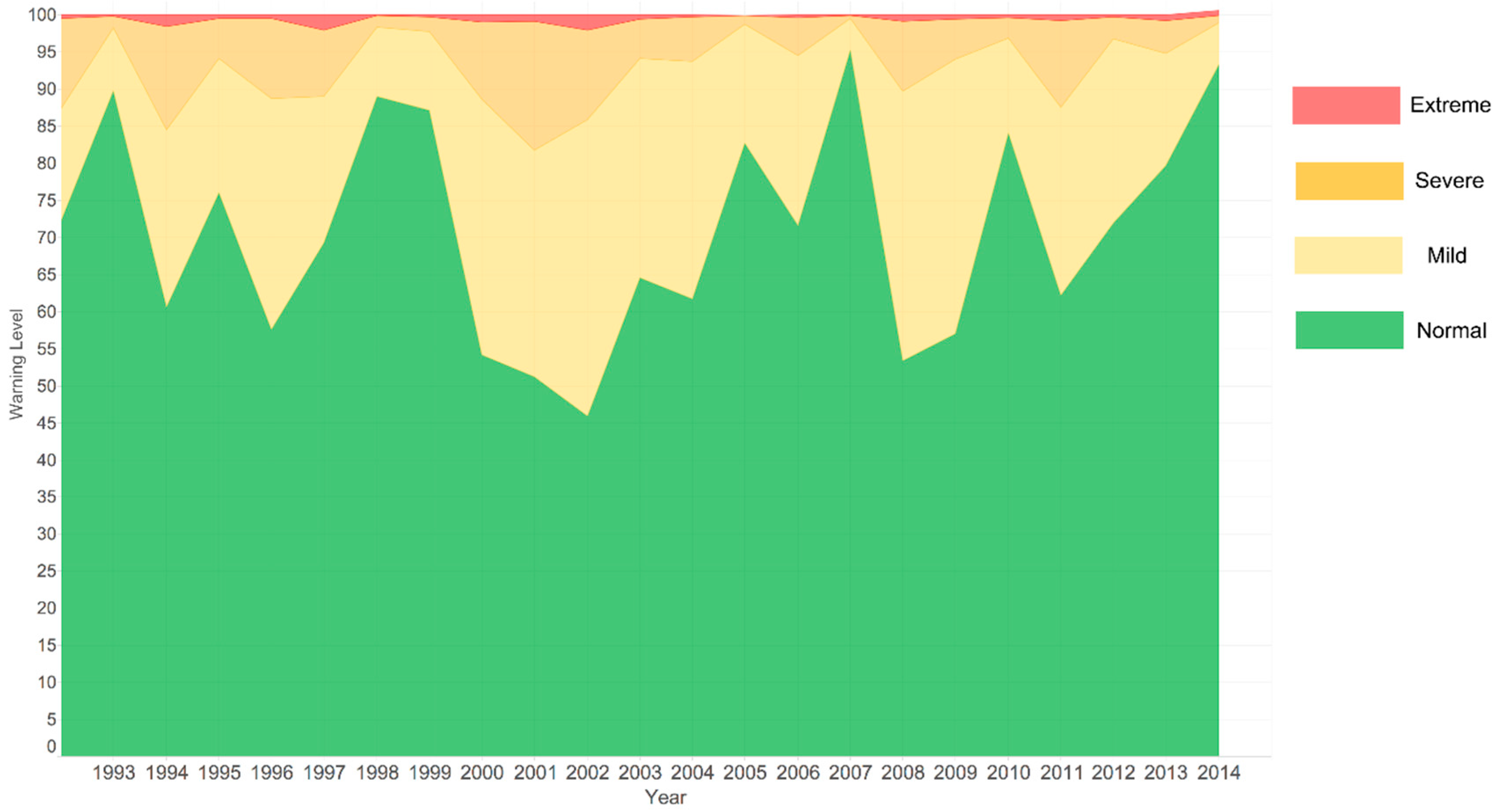
- We analyze the frequency of drought risk warning levels for each grid point and rank years according to the annual distribution of warning levels (Section 4.1).
- -
- We compare the ECDI-based drought risk warning levels to other (benchmark) drought monitoring indices (SPEI and scPDSI; Section 3.1.3), which are updated monthly. For this purpose, we resample the decadal warning levels to a monthly temporal resolution. Differences in spatial resolution are overcome via a nearest neighbor search. Afterwards, we analyze the agreement between the warning levels and the SPEI as well between the SPEI and the scPDSI (Section 4.2).
- -
- We validate the time series of all ECDI input variables, the corresponding climatology-based anomalies and the ECDI-based warning levels via reports of farmers in the Tigray region (Section 4.3). The farmers had reported moisture deficiencies during the start of season (SOS) in 2007, 2013, 2014 and 2015 which delayed the sowing/germination, and during the end of season (EOS) in 2007, which prohibited the development of fruits. All data were provided by the International Research Institute for Climate and Society (Columbia University).
4. Results and Discussion
4.1. Ranking Drought Years according to ECDI Warning Levels
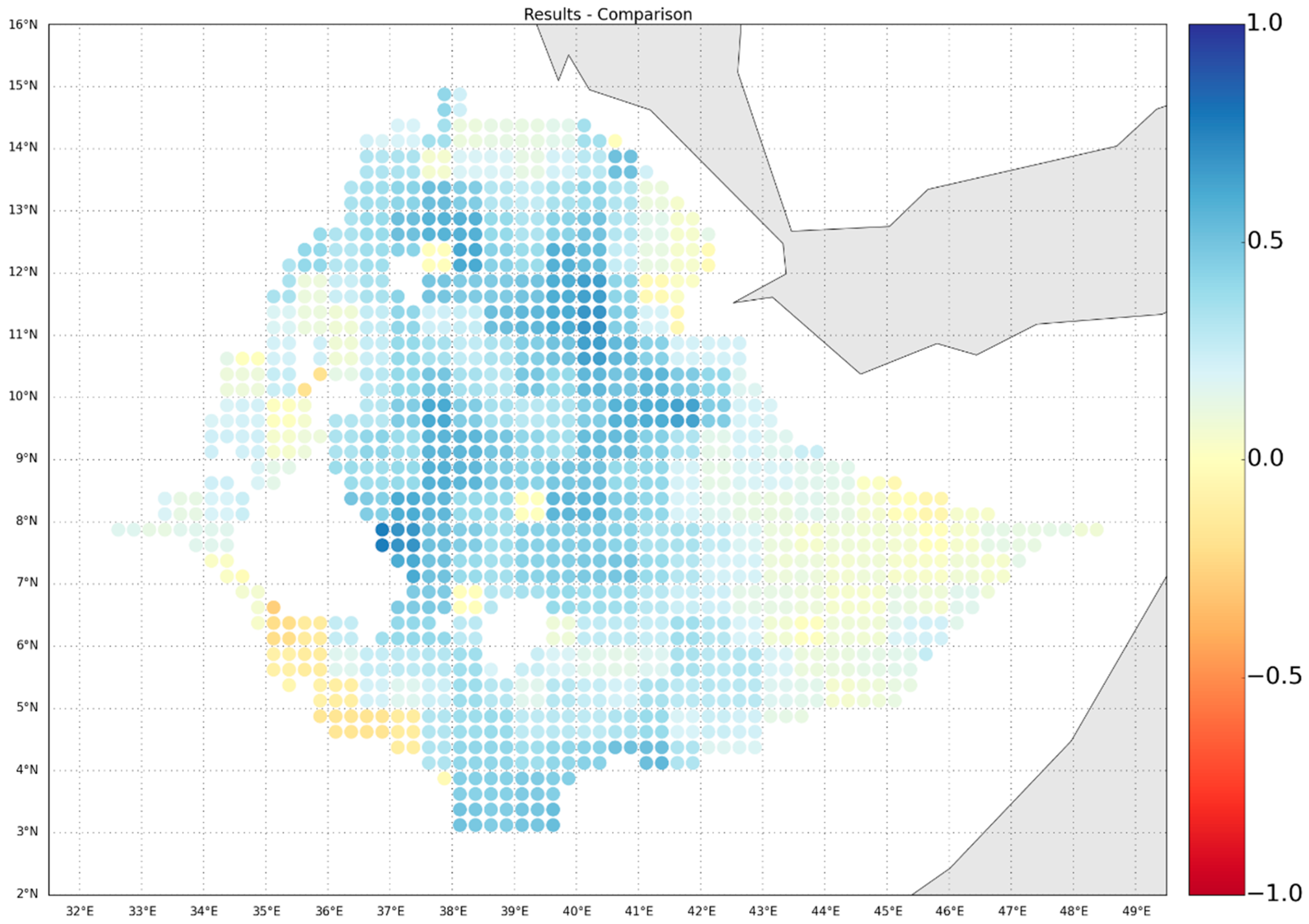
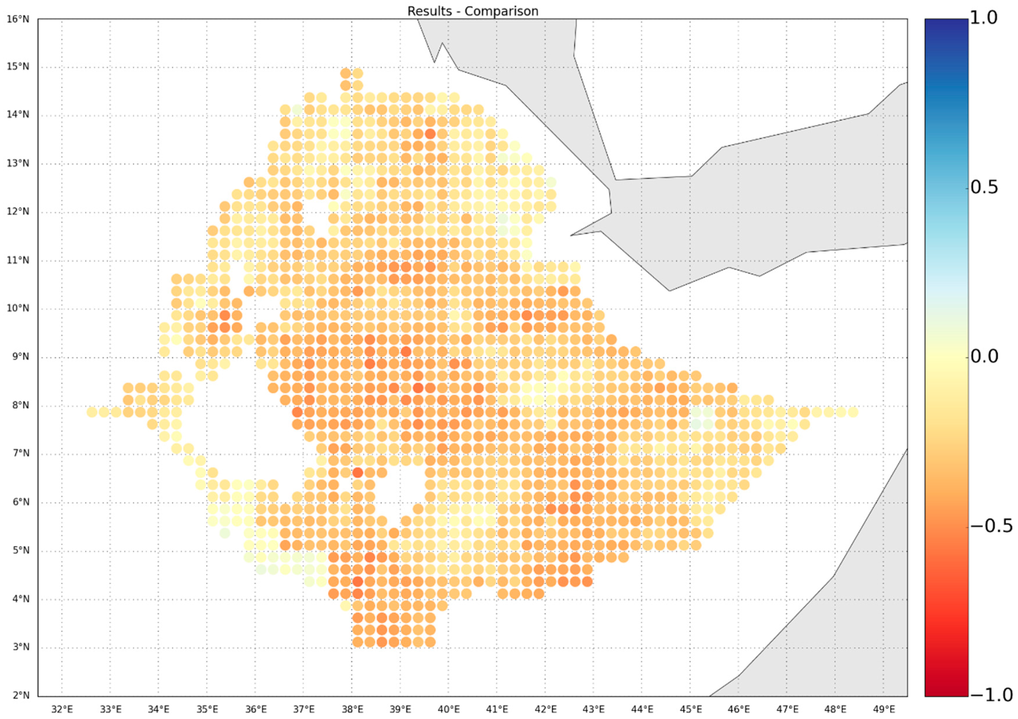
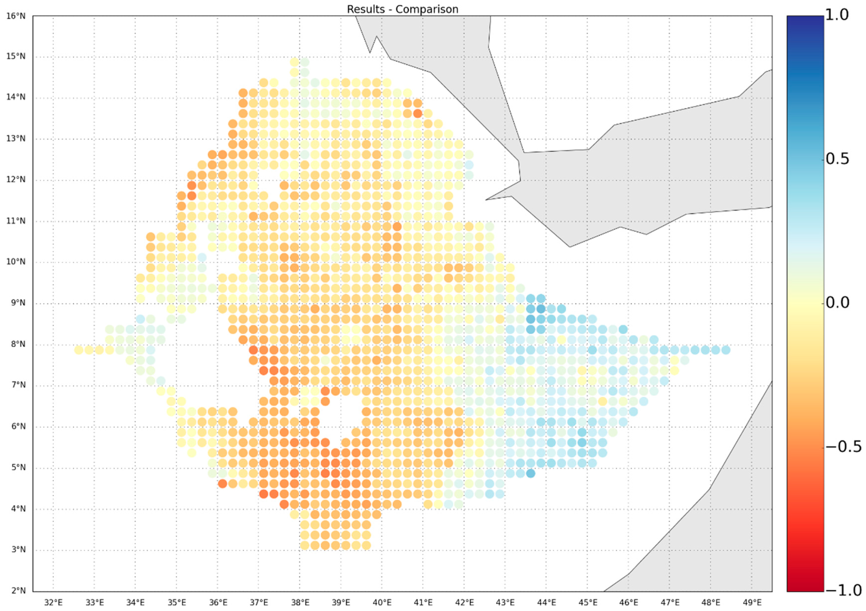
4.2. Large-Scale Comparison to SPEI and sc-PDSI
- -
- ScPDSI vs. SPEI (1992 to 2015);
- -
- ECDI-based warning levels vs. scPDSI (1992 to 2012); and
- -
- ECDI-based warning levels vs. SPEI (1992 to 2015).
4.3. Ground Truthing
4.3.1. Analysis of Raw Data and Anomalies
4.3.2. Drought Index Performance Metrics
4.3.3. Analysis of Warning Levels
4.4. Drought Forecasting
5. Conclusions and Outlook
Supplementary Materials
Acknowledgments
Author Contributions
Conflict of Interest
References
- Belal, A.-A.; El-Ramady, H.R.; Mohamed, E.S.; Saleh, A.M. Drought risk assessment using remote sensing and GIS techniques. Arab. J. Geosci. 2012, 7, 35–53. [Google Scholar] [CrossRef]
- Lloyd-Hughes, B. The impracticality of a universal drought definition. Theor. Appl. Climatol. 2014, 117, 607–611. [Google Scholar] [CrossRef]
- Overseas Development Institute Poverty and Poverty Reduction in Sub-Saharan Africa: An Overview of the Issues. Available online: http://www.odi.org/sites/odi.org.uk/files/odi-assets/publications-opinion-files/860.pdf (accessed on 14 October 2015).
- UN Food and Agriculture Organization. The State of Food Insecurity in the World—Meeting the 2015 International Hunger Targets: Taking Stock of Uneven Progress; UN Food and Agriculture Organization: Rome, Italy, 2015. [Google Scholar]
- UN Food and Agriculture Organization of the United Nations. The State of Food Insecurity in the World. High Food Prices and Food Security—Threats and Opportunities; UN Food and Agriculture Organization: Rome, Italy, 2008. [Google Scholar]
- Brown, M.E.; Funk, C.C. Food security under climate change. Science 2008, 319, 580–581. [Google Scholar] [CrossRef] [PubMed]
- Funk, C.C.; Brown, M.E. Declining global per capita agricultural production and warming oceans threaten food security. Food Secur. 2009, 1, 271–289. [Google Scholar] [CrossRef]
- United Nations Office for Disaster Risk Reduction (UNISDR). United Nations General Assembly Sendai Framework for Disaster Risk Reduction 2015–2030. In Proceedings of the Third United Nations World Conference on Disaster Risk Reduction, Sendai, Japan, 14–18 March 2015.
- Space-based Information for Disaster-Risk Reduction. Available online: http://www.un-spider.org/sites/default/files/Two_Pager_WCDRR_0.pdf (accessed on 22 June 2015).
- Verdin, J.; Funk, C.; Senay, G.; Choularton, R. Climate science and famine early warning. Philos. Trans. R. Soc. Lond. B Biol. Sci. 2005, 360, 2155–2168. [Google Scholar] [CrossRef] [PubMed]
- Rashid, A. Global Information and Early Warning System on Food and Agriculture: Appropriate Technology and Institutional Development Challenges. In Early Warning Systems for Natural Disaster Reduction; Zschau, P.D.J., Küppers, A., Eds.; Springer Berlin Heidelberg: Berlin, Germany; Heidelberg, Germany, 2003; pp. 337–344. [Google Scholar]
- Sheffield, J.; Wood, E.F.; Chaney, N.; Guan, K.; Sadri, S.; Yuan, X.; Olang, L.; Amani, A.; Ali, A.; Demuth, S.; et al. A Drought Monitoring and Forecasting System for Sub-Sahara African Water Resources and Food Security. Bull. Am. Meteorol. Soc. 2014, 95, 861–882. [Google Scholar] [CrossRef]
- Brown, M. Famine Early Warning Systems and Remote Sensing Data; Springer Berlin Heidelberg: Berlin, Germany; Heidelberg, Germany, 2008. [Google Scholar]
- Coughlan de Perez, E.; van den Hurk, B.; van Aalst, M.; Jongman, B.; Klose, T.; Suarez, P. Forecast-based financing: An approach for catalyzing humanitarian action based on extreme weather and climate forecasts. Nat. Hazards Earth Syst. Sci. Discuss 2014, 2, 3193–3218. [Google Scholar] [CrossRef]
- Kull, D.; Mechler, R.; Hochrainer-Stigler, S. Probabilistic cost-benefit analysis of disaster risk management in a development context. Disasters 2013, 37, 374–400. [Google Scholar] [CrossRef] [PubMed]
- Kellett, J.; Caravani, A. Financing Disaster Risk Reduction—A 20 Year Story of International Aid. Available online: http://www.odi.org/sites/odi.org.uk/files/odi-assets/publications-opinion-files/8574.pdf (accessed on 14 October 2015).
- Bachmair, S.; Kohn, I.; Stahl, K. Exploring the link between drought indicators and impacts. Nat. Hazards Earth Syst. Sci. 2015, 15, 1381–1397. [Google Scholar] [CrossRef]
- Wilhite, D.A.; Svoboda, M.D.; Hayes, M.J. Understanding the complex impacts of drought: A key to enhancing drought mitigation and preparedness. Water Resour. Manag. 2007, 21, 763–774. [Google Scholar] [CrossRef]
- United Nations Statistics Division UN Data Country Profiles 2014. Available online: http://data.un.org/CountryProfile.aspx (accessed on 14 October 2015).
- US Agency for International Development Ethiopia Agriculture and Food Security 2015. Available online: https://www.usaid.gov/ethiopia/agriculture-and-food-security (accessed on 14 October 2015).
- Peel, M.C.; Finlayson, B.L.; McMahon, T.A. Updated world map of the Köppen-Geiger climate classification. Hydrol. Earth Syst. Sci. 2007, 11, 1633–1644. [Google Scholar] [CrossRef]
- Alliance Development Works and United Nations University. World Risk Report 2014; Alliance Development Works: Berlin, Germany; United Nations University: Bonn, Germany, 2014. [Google Scholar]
- Naumann, G.; Barbosa, P.; Garrote, L.; Iglesias, A.; Vogt, J. Exploring drought vulnerability in Africa: An indicator based analysis to be used in early warning systems. Hydrol. Earth Syst. Sci. 2014, 18, 1591–1604. [Google Scholar] [CrossRef]
- Funk, C.; Dettinger, M.D.; Michaelsen, J.C.; Verdin, J.P.; Brown, M.E.; Barlow, M.; Hoell, A. Warming of the Indian Ocean threatens eastern and southern African food security but could be mitigated by agricultural development. Proc. Natl. Acad. Sci. USA 2008, 105, 11081–11086. [Google Scholar] [CrossRef] [PubMed]
- Clay, J.W.; Holcomb, B.K. Politics and the Ethiopian Famine: 1984–1985; Transaction Publishers: Cambridge, MA, USA, 1985. [Google Scholar]
- Hillbruner, C.; Moloney, G. When early warning is not enough—Lessons learned from the 2011 Somalia Famine. Glob. Food Secur. 2012, 1, 20–28. [Google Scholar] [CrossRef]
- Funk, C. We thought trouble was coming. Nat. News 2011, 476. [Google Scholar] [CrossRef] [PubMed]
- Maidment, R.I.; Grimes, D.; Allan, R.P.; Tarnavsky, E.; Stringer, M.; Hewison, T.; Roebeling, R.; Black, E. The 30 year TAMSAT African Rainfall Climatology and Time series (TARCAT) data set. J. Geophys. Res. Atmos. 2014, 119. [Google Scholar] [CrossRef]
- Tarnavsky, E.; Grimes, D.; Maidment, R.; Black, E.; Allan, R.P.; Stringer, M.; Chadwick, R.; Kayitakire, F. Extension of the TAMSAT Satellite-Based Rainfall Monitoring over Africa and from 1983 to Present. J. Appl. Meteorol. Climatol. 2014, 53, 2805–2822. [Google Scholar] [CrossRef]
- Wan, Z. New refinements and validation of the MODIS Land-Surface Temperature/Emissivity products. Remote Sens. Environ. 2008, 112, 59–74. [Google Scholar] [CrossRef]
- Balint, Z.; Mutua, F.M.; Muchiri, P. Drought Monitoring with the Combined Drought Index; FAO-SWALIM: Nairobi, Kenya, 2011. [Google Scholar]
- Palmer, W.C. Meteorological Drought; US Department of Commerce: Washington, DC, USA, 1965.
- Wells, N.; Goddard, S.; Hayes, M.J. A Self-Calibrating Palmer Drought Severity Index. J. Clim. 2004, 17, 2335–2351. [Google Scholar] [CrossRef]
- Vicente-Serrano, S.M.; Beguería, S.; López-Moreno, J.I. A Multiscalar Drought Index Sensitive to Global Warming: The Standardized Precipitation Evapotranspiration Index. J. Clim. 2010, 23, 1696–1718. [Google Scholar] [CrossRef]
- AghaKouchak, A. A baseline probabilistic drought forecasting framework using Standardized Soil Moisture Index: Application to the 2012 United States drought. Hydrol. Earth Syst. Sci. 2014, 18, 2485–2492. [Google Scholar] [CrossRef]
- Qiu, J.; Crow, W.T.; Nearing, G.S.; Mo, X.; Liu, S. The impact of vertical measurement depth on the information content of soil moisture times series data. Geophys. Res. Lett. 2014. [Google Scholar] [CrossRef]
- El Sharif, H.; Wang, J.; Georgakakos, A.P. Modeling Regional Crop Yield and Irrigation Demand Using SMAP Type of Soil Moisture Data. J. Hydrometeorol. 2015, 16, 904–916. [Google Scholar] [CrossRef]
- Kumar, S.V.; Harrison, K.W.; Peters-Lidard, C.D.; Santanello, J.A.; Kirschbaum, D. Assessing the Impact of L-Band Observations on Drought and Flood Risk Estimation: A Decision-Theoretic Approach in an OSSE Environment. J. Hydrometeorol. 2014, 15, 2140–2156. [Google Scholar] [CrossRef]
- McKee, T.B.; Doesken, N.J.; Kleist, J. The Relationship of Drought Frequency and Duration to time Scales. In Proceedings of the Eighth Conference on Applied Climatology, Anaheim, CA, USA, 17–22 January 1993.
- Tucker, C.J. Red and photographic infrared linear combinations for monitoring vegetation. Remote Sens. Environ. 1979, 8, 127–150. [Google Scholar] [CrossRef]
- Dai, A. Characteristics and trends in various forms of the Palmer Drought Severity Index during 1900–2008. J. Geophys. Res. 2011, 116. [Google Scholar] [CrossRef]
- Otkin, J.A.; Anderson, M.C.; Hain, C.; Mladenova, I.E.; Basara, J.B.; Svoboda, M. Examining Rapid Onset Drought Development Using the Thermal Infrared–Based Evaporative Stress Index. J. Hydrometeorol. 2013, 14, 1057–1074. [Google Scholar] [CrossRef]
- Anderson, M.C.; Zolin, C.A.; Sentelhas, P.C.; Hain, C.R.; Semmens, K.; Tugrul Yilmaz, M.; Gao, F.; Otkin, J.A.; Tetrault, R. The Evaporative Stress Index as an indicator of agricultural drought in Brazil: An assessment based on crop yield impacts. Remote Sens. Environ. 2016, 174, 82–99. [Google Scholar] [CrossRef]
- Dinku, T.; Ceccato, P.; Grover-Kopec, E.; Lemma, M.; Connor, S.J.; Ropelewski, C.F. Validation of satellite rainfall products over East Africa’s complex topography. Int. J. Remote Sens. 2007, 28, 1503–1526. [Google Scholar] [CrossRef]
- Thiemig, V.; Rojas, R.; Zambrano-Bigiarini, M.; Levizzani, V.; De Roo, A. Validation of Satellite-Based Precipitation Products over Sparsely Gauged African River Basins. J. Hydrometeorol. 2012, 13, 1760–1783. [Google Scholar] [CrossRef]
- The World Bank Turn down the Heat. Why a 4 °C Warmer World Must Be Avoided; The World Bank: Washington, DC, USA, 2012. [Google Scholar]
- Liu, Y.Y.; Dorigo, W.A.; Parinussa, R.M.; de Jeu, R.A.M.; Wagner, W.; McCabe, M.F.; Evans, J.P.; van Dijk, A.I.J.M. Trend-preserving blending of passive and active microwave soil moisture retrievals. Remote Sens. Environ. 2012, 123, 280–297. [Google Scholar] [CrossRef]
- Liu, Y.; Parinussa, R.M.; Dorigo, W.A.; De Jeu, R.A.M.; Wagner, W.; van Dijk, A.I.J.M.; McCabe, M.F.; Evans, J.P. Developing an improved soil moisture dataset by blending passive and active microwave satellite-based retrievals. Hydrol. Earth Syst. Sci. 2011, 15, 425–436. [Google Scholar] [CrossRef]
- Wagner, W.; Dorigo, W.; De Jeu, R.A.M.; Fernandez, D.; Benveniste, J.; Haas, E.; Ertl, M. Fusion of Active and Passive Microwave Observations to create an Essential Climate Variable Data Record on Soil Moisture. In ISPRS Annals of the Photogrammetry, Remote Sensing and Spatial Information Sciences; ISPRS: Melbourne, Australia, 2012; Volume I-7. [Google Scholar]
- McNally, A.; Shukla, S.; Arsenault, K.R.; Wang, S.; Peters-Lidard, C.D.; Verdin, J.P. Evaluating ESA CCI soil moisture in East Africa. Int. J. Appl. Earth Obs. Geoinf. 2016, 48, 96–109. [Google Scholar] [CrossRef]
- Li, X.; Zhang, L.; Weihermuller, L.; Jiang, L.; Vereecken, H. Measurement and Simulation of Topographic Effects on Passive Microwave Remote Sensing Over Mountain Areas: A Case Study From the Tibetan Plateau. IEEE Trans. Geosci. Remote Sens. 2014, 52, 1489–1501. [Google Scholar] [CrossRef]
- Wagner, W.; Hahn, S.; Kidd, R.; Melzer, T.; Bartalis, Z.; Hasenauer, S.; Figa-Saldaña, J.; de Rosnay, P.; Jann, A.; Schneider, S.; et al. The ASCAT Soil Moisture Product: A Review of its Specifications, Validation Results, and Emerging Applications. Meteorol. Z. 2013, 22, 5–33. [Google Scholar] [CrossRef]
- Anyamba, A.; Tucker, C.J. Analysis of Sahelian vegetation dynamics using NOAA-AVHRR NDVI data from 1981–2003. J. Arid Environ. 2005, 63, 596–614. [Google Scholar] [CrossRef]
- Rembold, F.; Atzberger, C.; Savin, I.; Rojas, O. Using Low Resolution Satellite Imagery for Yield Prediction and Yield Anomaly Detection. Remote Sens. 2013, 5, 1704–1733. [Google Scholar] [CrossRef]
- Atzberger, C. Advances in Remote Sensing of Agriculture: Context Description, Existing Operational Monitoring Systems and Major Information Needs. Remote Sens. 2013, 5, 949–981. [Google Scholar] [CrossRef]
- De Leeuw, J.; Vrieling, A.; Shee, A.; Atzberger, C.; Hadgu, K.M.; Biradar, C.M.; Keah, H.; Turvey, C. The Potential and Uptake of Remote Sensing in Insurance: A Review. Remote Sens. 2014, 6, 10888–10912. [Google Scholar] [CrossRef]
- Tadesse, T.; Demisse, G.B.; Zaitchik, B.; Dinku, T. Satellite-based hybrid drought monitoring tool for prediction of vegetation condition in Eastern Africa: A case study for Ethiopia. Water Resour. Res. 2014, 50, 2176–2190. [Google Scholar] [CrossRef]
- Nicholson, S.E.; Davenport, M.L.; Malo, A.R. A comparison of the vegetation response to rainfall in the Sahel and East Africa, using normalized difference vegetation index from NOAA AVHRR. Clim. Chang. 1990, 17, 209–241. [Google Scholar] [CrossRef]
- Herrmann, S.M.; Anyamba, A.; Tucker, C.J. Recent trends in vegetation dynamics in the African Sahel and their relationship to climate. Glob. Environ. Chang. 2005, 15, 394–404. [Google Scholar] [CrossRef]
- D’Odorico, P.; Caylor, K.; Okin, G.S.; Scanlon, T.M. On soil moisture–vegetation feedbacks and their possible effects on the dynamics of dryland ecosystems. J. Geophys. Res. Biogeosci. 2007, 112. [Google Scholar] [CrossRef]
- Jamali, S. Investigating Temporal Relationships between Rainfall, Soil Moisture and MODIS-Derived NDVI and EVI for Six Sites in Africa. Available online: http://www.isprs.org/proceedings/2011/ISRSE-34/211104015Final00443.pdf (accessed on 14 October 2015).
- Wang, J.; Rich, P.M.; Price, K.P. Temporal responses of NDVI to precipitation and temperature in the central Great Plains, USA. Int. J. Remote Sens. 2003, 24, 2345–2364. [Google Scholar] [CrossRef]
- Schnur, M.T.; Xie, H.; Wang, X. Estimating root zone soil moisture at distant sites using MODIS NDVI and EVI in a semi-arid region of southwestern USA. Ecol. Inform. 2010, 5, 400–409. [Google Scholar] [CrossRef]
- Ji, L.; Peters, A.J. Lag and seasonality considerations in evaluating AVHRR NDVI response to precipitation. Photogramm. Eng. Remote Sens. 2005, 71, 1053–1061. [Google Scholar] [CrossRef]
- Nandintsetseg, B.; Shinoda, M.; Kimura, R.; Ibaraki, Y. Relationship between Soil Moisture and Vegetation Activity in the Mongolian Steppe. Sci. Online Lett. Atmos. SOLA 2010, 6, 29–32. [Google Scholar] [CrossRef]
- Zribi, M.; Paris Anguela, T.; Duchemin, B.; Lili, Z.; Wagner, W.; Hasenauer, S.; Chehbouni, A. Relationship between soil moisture and vegetation in the Kairouan plain region of Tunisia using low spatial resolution satellite data. Water Resour. Res. 2010, 46, 823–835. [Google Scholar] [CrossRef]
- Atkinson, P.M.; Jeganathan, C.; Dash, J.; Atzberger, C. Inter-comparison of four models for smoothing satellite sensor time-series data to estimate vegetation phenology. Remote Sens. Environ. 2012, 123, 400–417. [Google Scholar] [CrossRef]
- Rembold, F.; Meroni, M.; Urbano, F.; Royer, A.; Atzberger, C.; Lemoine, G.; Eerens, H.; Haesen, D. Remote sensing time series analysis for crop monitoring with the SPIRITS software: New functionalities and use examples. Environ. Inform. 2015, 3, 1–11. [Google Scholar] [CrossRef]
- Atzberger, C.; Eilers, P.H.C. A time series for monitoring vegetation activity and phenology at 10-daily time steps covering large parts of South America. Int. J. Digit. Earth 2011, 4, 365–386. [Google Scholar] [CrossRef]
- Eilers, P.H.C. A Perfect Smoother. Anal. Chem. 2003, 75, 3631–3636. [Google Scholar] [CrossRef] [PubMed]
- Klisch, A.; Atzberger, C.; Luminari, L. Satellite-based drought monitoring in Kenya in an operational setting. ISPRS Int. Arch. Photogramm. Remote Sens. Spat. Inf. Sci. 2015, XL-7/W3, 433–439. [Google Scholar] [CrossRef]
- Vuolo, F.; Mattiuzzi, M.; Klisch, A.; Atzberger, C. Data Service Platform for MODIS Vegetation Indices Time Series Processing at BOKU Vienna: Current Status and Future Perspectives; Michel, U., Civco, D.L., Ehlers, M., Schulz, K., Nikolakopoulos, K.G., Habib, S., Messinger, D., Maltese, A., Eds.; SPIE: Vienna, Austria, 2012. [Google Scholar]
- Atzberger, C.; Eilers, P.H.C. Evaluating the effectiveness of smoothing algorithms in the absence of ground reference measurements. Int. J. Remote Sens. 2011, 32, 3689–3709. [Google Scholar] [CrossRef]
- Klisch, A.; Atzberger, C. Operational Drought Monitoring in Kenya Using MODIS NDVI Time Series. Remote Sens. 2016, 8. [Google Scholar] [CrossRef]
- Mistelbauer, T.; Enenkel, M.; Wagner, W. POETS—Python Open Earth Observation Tools, Poster: GIScience 2014. Available online: http://pub-geo.tuwien.ac.at/showentry.php?ID=231873&lang=6&nohtml=1 (accessed on 14 October 2015).
- Balint, Z.; Mutua, F.; Muchiri, P.; Omuto, C.T. Monitoring Drought with the Combined Drought Index in Kenya. In Developments in Earth Surface Processes; Elsevier B.V.: Amsterdam, The Netherlands, 2013; Volume 16, pp. 341–356. [Google Scholar]
- Berhan, G.; Tadesse, T.; Atnafu, S.; Hill, S. Drought Monitoring in Food-Insecure Areas of Ethiopia by Using Satellite Technologies. In Experiences of Climate Change Adaptation in Africa; Leal Filho, W., Ed.; Springer Berlin Heidelberg: Berlin, Germany; Heidelberg, Germany, 2011; pp. 183–200. [Google Scholar]
- UK Met Office How to Use Our Long-Range Predictions. Available online: http://www.metoffice.gov.uk/research/climate/seasonal-to-decadal/long-range/user-guide (accessed on 31 July 2014).
- Molteni, F.; Stockdale, T.; Balmaseda, M.; Balsamo, G.; Buizza, R.; Ferranti, L.; Magnusson, L.; Mogensen, K.; Palmer, T.; Vitard, F. The New ECMWF Seasonal Forecasting System (System 4). In ECMWF Technical Memorandum (Technical Report), No. 656; European Centre for Medium-Range Weather Forecasts: Reading, UK, 2011. [Google Scholar]
- Gneiting, T. Calibration of Medium-Range Weather Forecasts, ECMWF Technical Memorandum; European Centre for Medium-Range Weather Forecasts: Reading, UK, 2014; Volume 719. [Google Scholar]
- Reliefweb Ethiopia Drought Fact Sheet #1 (FY200). Available online: http://reliefweb.int/report/ethiopia/ethiopia-drought-fact-sheet-1-fy-2000 (accessed on 14 October 2015).
- UN Food and Agriculture Organization. Special Report FAO/FWP Crop and Food Supply Assessment Mission to Ethiopia 2001. Available online: http://www.fao.org/docrep/004/x9320e/x9320e00.HTM (accessed on 14 October 2015).
- UN Food and Agriculture Organization Ethiopia. Drought-Hit Farmers Receive Emergency Aid—Pre-Famine Conditions in Pockets of the Country. 2003. Available online: http://www.fao.org/english/newsroom/news/2003/18548-en.html (accessed on 5 May 2015).
- Meze-Hausken, E. Contrasting climate variability and meteorological drought with perceived drought and climate change in northern Ethiopia. Clim. Res. 2004, 27, 19–31. [Google Scholar] [CrossRef]
- UN Food and Agriculture Organization Ethiopia. El Niño-Southern Oscillation (ENSO) and the Main Kiremt Rainy Season—An Assessment Using FAO’s Agriculture Stress Index System (ASIS); UN Food and Agriculture Organization Ethiopia: Bole Subcity, Ethiopia, 2014. [Google Scholar]
- Zhao, H.; Gao, G.; An, W.; Zou, X.; Li, H.; Hou, M. Timescale differences between SC-PDSI and SPEI for drought monitoring in China. Phys. Chem. Earth Parts ABC 2015, in press. [Google Scholar] [CrossRef]
- Hane, D.C.; Pumphrey, F.V. Crop Water Use Curves for Irrigation Scheduling; Agricultural Experiment, Station, Oregon State University: Corvallis, OR, USA, 1984. [Google Scholar]
- UN Emergencies Unit for Ethiopia. Livelihood disruption in cash crop and surplus producing areas—A situation analysis July 2002. Available online: http://reliefweb.int/sites/reliefweb.int/files/resources/FD6A0E2619E3ECBD85256C0C00642F45-undpeue-eth-31jul.pdf (accessed on 14 October 2015).
- Tucker, C.; Pinzon, J.; Brown, M.; Slayback, D.; Pak, E.; Mahoney, R.; Vermote, E.; El Saleous, N. An extended AVHRR 8-km NDVI dataset compatible with MODIS and SPOT vegetation NDVI data. Int. J. Remote Sens. 2005, 26, 4485–4498. [Google Scholar] [CrossRef]


| Food Security Level | Generally Food Secure | Borderline Food Insecure | Acute Food Crisis | Food/Humanitarian Emergency | Famine/Humanitarian Catastrophe |
|---|---|---|---|---|---|
| Sample Parameter (Food Access) | Adequate and stable | Borderline adequate/seasonal Variations | Lack of sources (food, labor, cash) to ensure food access | Severe lack of sources; unable to meet food needs | Extreme lack of sources, starvation |
| Drought Risk Level | Normal Conditions | Increased Drought Risk | Severe Drought Risk | Extreme Drought Risk | |
| ECDI Warning Level | <−0.5 | −0.5 to −1.5 | −1.5 to −2.5 | >−2.5 STDV | |
| Indices | Period | Average Pearson’s R |
|---|---|---|
| scPDSI–SPEI | January–December | 0.28 |
| ECDI WL–scPDSI | January–December | −0.09 |
| ECDI WL–SPEI | January–December | −0.27 |
| scPDSI–SPEI | January–March | 0.34 |
| ECDI WL–scPDSI | January–March | −0.21 |
| ECDI WL–SPEI | January–March | −0.40 |
| scPDSI–SPEI | March–May (Belg season) | 0.34 |
| ECDI WL–scPDSI | March–May (Belg season) | −0.1 |
| ECDI WL–SPEI | March–May (Belg season) | −0.31 |
| scPDSI–SPEI | June–September (Kirempt season) | 0.24 |
| ECDI WL–scPDSI | June–September (Kirempt season) | −0.03 |
| ECDI WL–SPEI | June–September (Kirempt season) | −0.21 |
| scPDSI–SPEI | October–December | 0.25 |
| ECDI WL–scPDSI | October–December | −0.08 |
| ECDI WL–SPEI | October–December | −0.23 |
| Region | Drought Index 1 | Drought Index 2 | Location | R | R (June–September) | S | S (June–September) |
|---|---|---|---|---|---|---|---|
| R1 | scPDSI | SPEI | 39.72E/13.85N 39.59E/13.79N | 0.23 | 0.20 | 0.02 | 0.19 |
| R1 | ECDI WL | scPDSI | 39.72E/13.85N 39.59E/13.79N | −0.06 | 0.12 | 0.08 | 0.32 |
| R1 | ECDI WL | SPEI | 39.72E/13.85N 39.59E/13.79N | −0.38 | −0.30 | −0.43 | −0.36 |
| R2 | scPDSI | SPEI | 39.56E/14.1N | 0.15 | 0.10 | 0.09 | 0.21 |
| R2 | ECDI WL | scPDSI | 39.56E/14.1N | −0.21 | −0.08 | −0.23 | −0.14 |
| R2 | ECDI WL | SPEI | 39.56E/14.1N | −0.16 | −0.19 | −0.25 | −0.23 |
| R3 | scPDSI | SPEI | 39.5E/4.00N | 0.47 | 0.38 | 0.42 | 0.38 |
| R3 | ECDI WL | scPDSI | 39.5E/4.00N | −0.45 | -0.44 | −0.46 | −0.40 |
| R3 | ECDI WL | SPEI | 39.5E/4.00N | −0.41 | −0.53 | −0.43 | −0.45 |
| R4 | scPDSI | SPEI | 42.75E/4.75N | 0.25 | 0.36 | 0.30 | 0.15 |
| R4 | ECDI WL | scPDSI | 42.75E/4.75N | 0.23 | 0.42 | 0.26 | 0.47 |
| R4 | ECDI WL | SPEI | 42.75E/4.75N | −0.44 | −0.32 | −0.26 | −0.30 |
| R5 | scPDSI | SPEI | 46.0E/6.5N | 0.26 | 0.12 | 0.14 | −0.12 |
| R5 | ECDI WL | scPDSI | 46.0E/6.5N | 0.01 | −0.16 | 0.10 | −0.11 |
| R5 | ECDI WL | SPEI | 46.0E/6.5N | −0.18 | 0.05 | −0.07 | 0.01 |
| R6 | scPDSI | SPEI | 41.5E/7.5N | 0.40 | 0.07 | 0.42 | 0.05 |
| R6 | ECDI WL | scPDSI | 41.5E/7.5N | 0.0 | −0.06 | −0.02 | −0.04 |
| R6 | ECDI WL | SPEI | 41.5E/7.5N | −0.34 | −0.35 | −0.37 | −0.42 |
© 2016 by the authors; licensee MDPI, Basel, Switzerland. This article is an open access article distributed under the terms and conditions of the Creative Commons Attribution (CC-BY) license (http://creativecommons.org/licenses/by/4.0/).
Share and Cite
Enenkel, M.; Steiner, C.; Mistelbauer, T.; Dorigo, W.; Wagner, W.; See, L.; Atzberger, C.; Schneider, S.; Rogenhofer, E. A Combined Satellite-Derived Drought Indicator to Support Humanitarian Aid Organizations. Remote Sens. 2016, 8, 340. https://doi.org/10.3390/rs8040340
Enenkel M, Steiner C, Mistelbauer T, Dorigo W, Wagner W, See L, Atzberger C, Schneider S, Rogenhofer E. A Combined Satellite-Derived Drought Indicator to Support Humanitarian Aid Organizations. Remote Sensing. 2016; 8(4):340. https://doi.org/10.3390/rs8040340
Chicago/Turabian StyleEnenkel, Markus, Caroline Steiner, Thomas Mistelbauer, Wouter Dorigo, Wolfgang Wagner, Linda See, Clement Atzberger, Stefan Schneider, and Edith Rogenhofer. 2016. "A Combined Satellite-Derived Drought Indicator to Support Humanitarian Aid Organizations" Remote Sensing 8, no. 4: 340. https://doi.org/10.3390/rs8040340
APA StyleEnenkel, M., Steiner, C., Mistelbauer, T., Dorigo, W., Wagner, W., See, L., Atzberger, C., Schneider, S., & Rogenhofer, E. (2016). A Combined Satellite-Derived Drought Indicator to Support Humanitarian Aid Organizations. Remote Sensing, 8(4), 340. https://doi.org/10.3390/rs8040340