
Evaluating the Diurnal Cycle of Upper Tropospheric Humidity in Two Different Climate Models Using Satellite Observations


Abstract
:
1. Introduction
2. Satellite Data and Models
2.1. Satellite Data
2.2. Climate Models
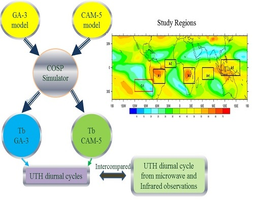
3. Methodology
3.1. Diurnal Cycle from Microwave Measurements
3.2. Diurnal Cycle from IR Measurements
3.3. Diurnal Cycle from Models
4. Results and Discussion
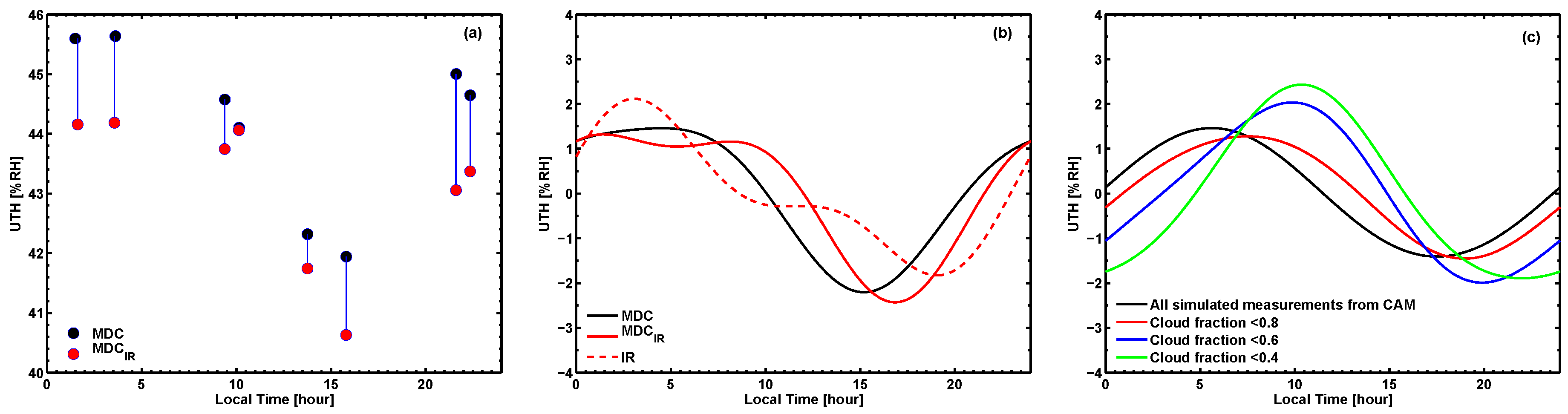
4.1. Differences between IR and Microwave Diurnal Cycle
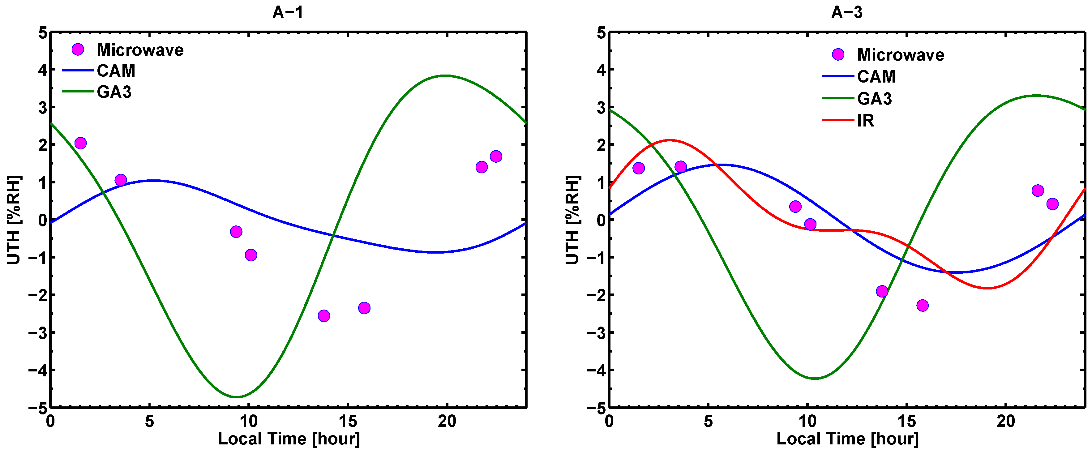
4.2. Diurnal Cycle in Models and Observations
5. Conclusions
Acknowledgments
Author Contributions
Conflicts of Interest
References
- Yang, G.Y.; Slingo, J. The diurnal cycle in the tropics. Mon. Weather Rev. 2000, 129, 784–801. [Google Scholar] [CrossRef]
- Soden, B.J. The diurnal cycle of convection, clouds, and water vapor in the tropical upper troposphere. Geophys. Res. Lett. 2000, 27, 2173–2176. [Google Scholar] [CrossRef]
- Soden, B.J. The impact of tropical convection and cirrus an upper tropospheric humidity: A lagrangian analysis of satellite measurements. Geophys. Res. Lett. 2004, 31. [Google Scholar] [CrossRef]
- Seidel, D.J.; Free, M.; Wang, J. Diurnal cycle of upper-air temperature estimated from radiosondes. J. Geophys. Res. (Atmos.) 2005, 110, D09102. [Google Scholar] [CrossRef]
- Miloshevich, L.M.; Vömel, H.; Whiteman, D.N.; Leblanc, T. Accuracy assessment and correction of vaisala RS92 radiosonde water vapor measurements. J. Geophys. Res. 2009, 114, D11305. [Google Scholar] [CrossRef]
- Kottayil, A.; Buehler, S.A.; John, V.O.; Miloshevich, L.M.; Milz, M.; Holl, G. On the importance of Vaisala RS92 radiosonde humidity corrections for a better agreement between measured and modeled satellite radiances. J. Atmos. Oceanic Technol. 2012, 29, 248–259. [Google Scholar] [CrossRef]
- Soden, B.J.; Bretherton, F.P. Interpretation of TOVS water vapor radiances in terms of layer-average relative humidities: Method and climatology for the upper, middle, and lower troposphere. J. Geophys. Res. 1996, 101, 9333–9343. [Google Scholar] [CrossRef]
- Buehler, S.A.; Kuvatov, M.; John, V.O.; Milz, M.; Soden, B.J.; Jackson, D.L.; Notholt, J. An upper tropospheric humidity data set from operational satellite microwave data. J. Geophys. Res. 2008, 113, D14110. [Google Scholar] [CrossRef]
- John, V.O.; Soden, B.J. Temperature and humidity biases in global climate models and their impact on climate feedbacks. Geophys. Res. Lett. 2007, 34, L18704. [Google Scholar] [CrossRef]
- Iacono, M.J.; Delamere, J.S.; Mlawer, E.J.; Clough, S.A. Evaluation of upper tropospheric water vapor in the NCAR Community Climate Model (CCM3) using modeled and observed HIRS radiances. J. Geophys. Res.: Atmos. 2003, 108, 4037. [Google Scholar] [CrossRef]
- Allan, R.P.; Ringer, M.A.; Slingo, A. Evaluation of moisture in the Hadley Centre climate model using simulations of HIRS water-vapor channel radiances. Q. J. R. Meteorol. Soc. 2003, 129, 3371–3389. [Google Scholar] [CrossRef]
- Gettelman, A.; Collins, W.D.; Fetzer, E.J.; Eldering, A.; Irion, F.W.; Duffy, P.B.; Bala, G. Climatology of upper-tropospheric relative humidity from the atmospheric infrared sounder and implications for climate. J. Clim. 2006, 19, 6104–6121. [Google Scholar] [CrossRef]
- Spangenberg, D.A.; Mace, G.G.; Ackerman, T.P.; Seaman, N.L.; Soden, B.J. Evaluation of model-simulated upper troposphere humidity using 6.7 μm satellite observations. J. Geophys. Res. 1997, 102, 25737–25749. [Google Scholar] [CrossRef]
- Tian, B.; Fetzer, E.J.; Kahn, B.H.; Teixeira, J.; Manning, E.; Hearty, T. Evaluating CMIP5 models using AIRS tropospheric air temperature and specific humidity climatology. J. Geophys. Res.: Atmos. 2013, 118, 114–134. [Google Scholar] [CrossRef]
- Jiang, J.H.; Su, H.; Zhai, C.; Perun, V.; del Genio, A.D.; Nazarenko, L.S.; Donner, L.J.; Horowitz, L.W.; Seman, C.J.; Cole, J. Evaluation of cloud and water vapor simulations in CMIP5 climate models using NASA A-Train satellite observations. J. Geophys. Res.: Atmos. 2012, 117, D14105. [Google Scholar] [CrossRef]
- Slingo, A.; Hodges, K.I.; Robinson, G.J. Simulation of the diurnal cycle in a climate model and its evaluation using data from Meteosat 7. Q. J. R. Meteorol. Soc. 2004, 130, 1449–1467. [Google Scholar] [CrossRef]
- MacKenzie, I.A.; Tett, S.F.B.; Lindfors, A.V. Climate model-simulated diurnal cycles in HIRS clear-sky brightness temperatures. J. Clim. 2012, 25, 5845–5863. [Google Scholar] [CrossRef]
- Zhang, Y.; Klein, S.A.; Liu, C.; Tian, B.; Marchand, R.T.; Haynes, J.M.; McCoy, R.B.; Zhang, Y.; Ackerman, T.P. On the diurnal cycle of deep convection, high-level cloud, and upper troposphere water vapor in the Multiscale Modeling Framework. J. Geophys. Res. 2008, 113, D16105. [Google Scholar] [CrossRef]
- Eriksson, P.; Rydberg, B.; Johnston, M.; Murtagh, D.P.; Struthers, H.; Ferrachat, S.; Lohmann, U. Diurnal variations of humidity and ice water content in the tropical upper troposphere. Atmos. Chem. Phys. 2010, 10, 11519–11533. [Google Scholar] [CrossRef]
- Chung, E.-S.; Soden, B.J.; Sohn, B.J.; Schmetz, J. An assessment of the diurnal variation of upper tropospheric humidity in reanalysis data sets. J. Geophys. Res.: Atmos. 2013, 118, 3425–3430. [Google Scholar] [CrossRef]
- Eriksson, P.; Rydberg, B.; Sagawa, H.; Johnston, M.S.; Kasai, Y. Overview and sample applications of SMILES and Odin-SMR retrievals of upper tropospheric humidity and cloud ice mass. Atmos. Chem. Phys. 2014, 14, 12613–12629. [Google Scholar] [CrossRef]
- Saunders, R.W.; Hewison, T.J.; Stringer, S.J.; Atkinson, N.C. The radiometric characterization of AMSU-B. IEEE Trans. Microw. Theory 1995, 43, 760–771. [Google Scholar] [CrossRef]
- Bonsignori, R. The Microwave Humidity Sounder (MHS): In-orbit performance assessment. Proc. SPIE 2007. [Google Scholar] [CrossRef]
- John, V.O.; Holl, G.; Atkinson, N.; Buehler, S.A. Monitoring scan asymmetry of microwave humidity sounding channels using simultaneous all angle collocations (SAACs). J. Geophys. Res. 2013. [Google Scholar] [CrossRef]
- Brogniez, H.; Roca, R.; Picon, L. A clear-sky radiance archive from Meteosat “water vapor” observations. J. Geophys. Res. 2006, 111, D21109. [Google Scholar] [CrossRef]
- Gettelman, A.; Morrison, H.; Ghan, S.J. A new two-moment bulk stratiform cloud microphysics scheme in the Community Atmosphere Model, version 3 (CAM3). Part II: Single-column and global results. J. Clim. 2008, 21, 3660. [Google Scholar] [CrossRef]
- Gettelman, A.; Liu, X.; Ghan, S.J.; Morrison, H.; Park, S.; Conley, A.J.; Klein, S.A.; Boyle, J.; Mitchell, D.L.; Li, J.-L.F. Global simulations of ice nucleation and ice supersaturation with an improved cloud scheme in the community atmosphere model. J. Geophys. Res. 2010, 115. [Google Scholar] [CrossRef]
- Neale, R.B.; Richter, J.H.; Conley, A.J.; Park, S.; Lauritzen, P.H.; Gettelman, A.; Williamson, D.L.; Rasch, P.J.; Vavrus, S.J.; Taylor, M.A.; et al. Description of the NCAR Community Atmosphere Model (CAM 5.0); NCAR Technical Note; NCAR: Boulder, CO, USA, 2010. [Google Scholar]
- Walters, D.N.; Best, M.J.; Bushell, A.C.; Copsey, D.; Edwards, J.M.; Falloon, P.D.; Harris, C.M.; Lock, A.P.; Manners, J.C.; Morcrette, C.J.; et al. The met office unified model global atmosphere 3.0/3.1 and jules global land 3.0/3.1 configurations. Geosci. Model Dev. 2011, 4, 919–941. [Google Scholar] [CrossRef]
- Taylor, K.E.; Stouffer, R.J.; Meehl, G.A. An Overview of CMIP5 and the Experiment Design. Bull. Am. Meteorol. Soc. 2012, 93, 485–498. [Google Scholar] [CrossRef]
- Kottayil, A.; John, V.O.; Buehler, S.A. Correcting diurnal cycle aliasing in satellite microwave humidity sounder measurements. J. Geophys. Res. 2013, 118, 101–113. [Google Scholar] [CrossRef]
- Buehler, S.A.; Kuvatov, M.; Sreerekha, T.R.; John, V.O.; Rydberg, B.; Eriksson, P.; Notholt, J. A cloud filtering method for microwave upper tropospheric humidity measurements. Atmos. Chem. Phys. 2007, 7, 5531–5542. [Google Scholar] [CrossRef]
- Buehler, S.A.; John, V.O. A simple method to relate microwave radiances to upper tropospheric humidity. J. Geophys. Res. 2005, 110, D02110. [Google Scholar] [CrossRef]
- John, V.O.; Buehler, S.A.; Courcoux, N. A cautionary note on the use of gaussian statistics in satellite based UTH climatologies. IEEE Geosci. Remote Sens. Lett. 2006, 3, 130–134. [Google Scholar] [CrossRef]
- Lindfors, A.V.; MacKenzie, I.A.; Tett, S.F.B.; Shi, L. Climatological diurnal cycles in clear-sky brightness temperatures from the High-Resolution Infrared Radiation Sounder (HIRS). J. Atmos. Ocean. Technol. 2011, 28, 1199–1205. [Google Scholar] [CrossRef]
- John, V.O.; Allan, R.P.; Bell, B.; Buehler, S.A.; Kottayil, A. Assessment of inter-calibration methods for satellite microwave humidity sounders. J. Geophys. Res. 2013, 118, 1–13. [Google Scholar] [CrossRef]
- John, V.O.; Holl, G.; Allan, R.P.; Buehler, S.A.; Parker, D.E.; Soden, B.J. Clear-sky biases in satellite infra-red estimates of upper tropospheric humidity and its trends. J. Geophys. Res. 2011, 116, D14108. [Google Scholar] [CrossRef]
- Holl, G.; Buehler, S.A.; Rydberg, B.; Jiménez, C. Collocating satellite-based radar and radiometer measurements—Methodology and usage examples. Atmos. Meas. Tech. 2010, 3, 693–708. [Google Scholar] [CrossRef]
- Roca, R.; Brogniez, H.; Picon, L.; Desbois, M. High resolution observations of free tropopsheric humidity from METEOSAT over the indian ocean. In Proceedings of the 2nd MEGHA-TROPIQUES Scientific Workshop, Paris, France, 2–6 July 2001.
- Bodas-Salcedo, A.; Webb, M.J.; Bony, S.; Chepfer, H.; Dufresne, J.-L.; Klein, S.A.; Zhang, Y.; Marchand, R.; Haynes, J.M.; Pincus, R.; et al. COSP: Satellite simulation software for model assessment. Bull. Amer. Met. Soc. 2011, 92, 1023–1043. [Google Scholar] [CrossRef] [Green Version]
- Sohn, B.J.; Schmetz, J.; Tjemkes, S.; Koenig, M.; Lutz, H.; Arriaga, A.; Chung, E.S. Intercalibration of the Meteosat-7 water vapor channel with SSM/T-2. J. Geophys. Res.: Atmos. 2000, 105, 15673–15680. [Google Scholar] [CrossRef]
- Chung, E.S.; Sohn, B.J.; Schmetz, J.; Koenig, M. Diurnal variation of upper tropospheric humidity and its relations to convective activities over tropical africa. Atmos. Chem. Phys. 2007, 7, 2489–2502. [Google Scholar] [CrossRef]
- Tan, J.; Jakob, C. A three-hourly data set of the state of tropical convection based on cloud regimes. Geophys. Res. Lett. 2013, 40, 1415–1419. [Google Scholar] [CrossRef]
- Millan, L.; Read, W.; Kasai, Y.; Lambert, A.; Livesey, N.J.; Mendrok, A.; Sagawa, H.; Sano, T.; Shiotani, D.L.; Wu, M. SMILES ice cloud products. J. Geophys. Res.: Atmos. 2013, 118. [Google Scholar] [CrossRef]
- Jiang, J.H.; Su, H.; Zhai, C.; Shen, T.J.; Wu, T.; Zhang, J.; Cole, J.N.S.; von Salzen, K.; Donner, L.J.; Seman, C.; et al. Evaluating the diurnal cycle of Upper-tropospheric ice clouds in climate models using SMILES observations. J. Atmos. Sci. 2015, 72, 1022–1044. [Google Scholar] [CrossRef]
- Pierrehumbert, R.T.; Roca, R. Evidence for control of Atlantic subtropical humidity by large scale advection. Geophys. Res. Lett. 1998, 25, 4537–4540. [Google Scholar] [CrossRef]
- Kottayil, A.; Satheesan, K. Enhancement in the upper tropospheric humidity associated with aerosol loading over tropical pacific. Atmos. Environ. 2015, 122, 148–153. [Google Scholar] [CrossRef]
- Hoareau, C.; Keckhut, P.; Baray, J.-L.; Robert, L.; Courcoux, Y.; Porteneuve, J.; Vömel, H.; Morel, B. A Raman lidar at La Reunion (20.8°S, 55.5°E) for monitoring water vapor and cirrus distributions in the subtropical upper troposphere: Preliminary analyses and description of a future system. Atmos. Meas. Tech. 2012, 5, 1333–1348. [Google Scholar] [CrossRef]
- Hoareau, C.; Keckhut, P.; Noel, V.; Chepfer, H.; Baray, J.-L. A decadal cirrus clouds climatology from ground-based and spaceborne lidars above the south of France (43.9°N–5.7°E). Atmos. Chem. Phys. 2013, 13, 6951–6963. [Google Scholar] [CrossRef] [Green Version]


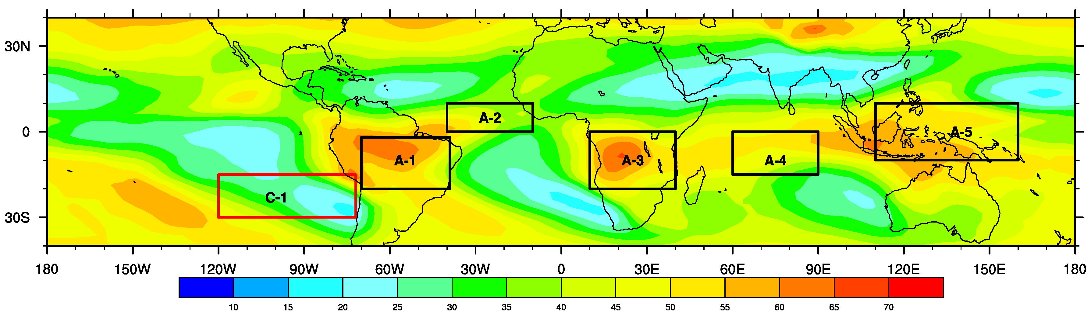
| Region | Location |
|---|---|
| South America (A-1) | 40W–70W; 5S–20S |
| Atlantic (A-2) | 10W–40W; 0–10N |
| Africa (A-3) | 10E–40E; 0–20S |
| Indian Ocean (A-4) | 60E–90E; 0–15S |
| West Pacific (A-5) | 110E–160E; 10N–10S |
| South East Pacific (C-1) | 70W–120W; 15S–30S |
| Region | Measured lag (h) | Model cf Threshold |
|---|---|---|
| A-1 | 1.2 | 0.72 |
| A-2 | 1.15 (3.50) | 0.52 |
| A-3 | 1.65 (3.00) | 0.78 |
| A-4 | 0.1 | 0.98 |
| A-5 | 0.1 | 0.76 |
| Tropics (25S–25N) | 1.55 | 0.56 |
| Region | Observation | GA-3 | CAM-5 | ||||||
|---|---|---|---|---|---|---|---|---|---|
| DUR | LTMAX | LTMIN | DUR | LTMAX | LTMIN | DUR | LTMAX | LTMIN | |
| A-1 | 4.5 | 2 | 14 | 7.5 | 20 | 9 | 2 | 5 | 19 |
| A-2 | 2 | 2 | 14 | 0.8 | 2 | 17 | 1.5 | 5 | 18 |
| A-3 | 3.5 | 2 | 16 | 7 | 22 | 10 | 2 | 5 | 18 |
| A-4 | 2 | 2 | 14 | 0.8 | 2 | 10 | 1.5 | 4 | 18 |
| A-5 | 2 | 22 | 14 | 1.2 | 2 | 11 | 2 | 7 | 18 |
© 2016 by the authors; licensee MDPI, Basel, Switzerland. This article is an open access article distributed under the terms and conditions of the Creative Commons by Attribution (CC-BY) license (http://creativecommons.org/licenses/by/4.0/).
Share and Cite
Kottayil, A.; John, V.O.; Buehler, S.A.; Mohanakumar, K. Evaluating the Diurnal Cycle of Upper Tropospheric Humidity in Two Different Climate Models Using Satellite Observations. Remote Sens. 2016, 8, 325. https://doi.org/10.3390/rs8040325
Kottayil A, John VO, Buehler SA, Mohanakumar K. Evaluating the Diurnal Cycle of Upper Tropospheric Humidity in Two Different Climate Models Using Satellite Observations. Remote Sensing. 2016; 8(4):325. https://doi.org/10.3390/rs8040325
Chicago/Turabian StyleKottayil, Ajil, Viju O. John, Stefan A. Buehler, and Kesavapillai Mohanakumar. 2016. "Evaluating the Diurnal Cycle of Upper Tropospheric Humidity in Two Different Climate Models Using Satellite Observations" Remote Sensing 8, no. 4: 325. https://doi.org/10.3390/rs8040325