Spatial Estimation of Classification Accuracy Using Indicator Kriging with an Image-Derived Ambiguity Index

Abstract

Traditional classification accuracy assessments based on summary statistics from a confusion matrix furnish a global (location invariant) view of classification accuracy. To estimate the spatial distribution of classification accuracy, a geostatistical integration approach is presented in this paper. Indicator kriging with local means is combined with logistic regression to integrate an image-derived ambiguity index with classification accuracy values at reference data locations. As for the ambiguity measure, a novel discrimination capability index (DCI) is defined from per class posteriori probabilities and then calibrated via logistic regression to derive soft probabilities. Integration of indicator-coded reference data with soft probabilities is finally carried out for mapping classification accuracy. It is demonstrated via a case study involving classification of multi-temporal and multi-sensor SAR datasets, that the proposed approach can provide a map of locally-varying accuracy values, while respecting the overall accuracy derived from the confusion matrix. It can also highlight areas where the benefit of data fusion was significant. It is expected that the indicator approach presented in this paper could be a useful methodology for assessing the spatial quality of classification results in a probabilistic way.

1. Introduction

Thematic mapping through classification of remote sensing data has been regarded as one of the most important application fields of remote sensing. Classification-derived area class maps, such as land use/cover and crop type maps, are routinely used as input data for various environmental modeling tasks, such as natural disaster prediction modeling, crop yield assessment, and spatial estimation of air pollution [1,2,3]. Since class maps are used as inputs into environmental models, any errors arising during classification may propagate to the applied model outputs, hence leading to error propagation problems [4]. Therefore, it is of critical importance to generate reliable classification results for further analysis. Many efforts have been made to improve classification accuracy by either developing advanced classification algorithms or using multi-source/sensor data [5,6,7,8,9,10,11,12,13]. The classification procedure for thematic mapping can also be regarded as the prediction of target classes prevailing at unsampled locations. Therefore, the development of methods for the accuracy assessment of classification results should be considered to be an equally important task in the classification procedure as the development of advanced classification algorithms.

Classification accuracy is traditionally reported in terms of several statistical measures derived from a confusion matrix, also called an error matrix [14,15]. Several accuracy statistics, such as overall accuracy, user’s accuracy, producer’s accuracy, and the Kappa coefficient, can be derived from the confusion matrix and have been widely used for evaluating the quality of classification results. However, such accuracy measures are global class-specific statistics; they pertain to all pixels of a given class and do not reveal any within-class spatial variation. It is, therefore, very difficult, or even impossible, to pinpoint areas where detailed ground surveys are needed within the limits of a particular class.

Several approaches have been proposed for spatial accuracy assessment or mapping classification accuracy distributions. The first approach uses the byproducts of soft classification directly as measures of map quality. Exaggeration and ignorance uncertainties based on fuzzy logic were proposed in [16]. Exaggeration uncertainty was defined as the deviation from unity of the membership values of the assigned class. Ignorance uncertainty quantified by an entropy measure was regarded as the degree of ignorance of other class memberships due to class assignment or hardening [16]. Although these two uncertainty measures are related to the spatial variation of classification uncertainty, they do not provide information on classification accuracy because reference data are not involved in the estimation procedure. Steele et al. [17] estimated misclassification probabilities by interpolating bootstrap estimates at training data locations via kriging. Reference data that are independent of the classification procedure are invaluable sources for accuracy assessment. Such data, however, were not used for estimating misclassification probabilities in this case. Kyriakidis and Dungan [18] presented two local indices of map quality, termed confusion and inaccuracy indices, by integrating reference data with soft probabilities computed from the user’s accuracy within an indicator geostatistical framework [19]. Since soft probabilities were derived based on the user’s accuracy, a global statistic, varying degrees of classification reliability and actual classification results (i.e., correct or incorrect classification) at reference data locations were not accounted for in the map quality indices.

In this study, a simple but efficient geostatistical approach is presented for the spatial estimation of classification accuracy by combining correct or incorrect classification results at reference data locations with exhaustive image-derived ambiguity information. The spatial distribution of classification accuracy is defined in this study as the probability of correct classification at any image pixel. That probability attains a binary value (1 or 0) at reference pixels, where true class labels are available and, hence, a pixel can be either correctly (1) or incorrectly classified. Other pixels, except the reference pixels, have the probability between 0 and 1. The term “classification accuracy probability” will be used as above probability of correct classification throughout this paper. Under the assumption that classification accuracy probability is related to ambiguity or uncertainty involved in the class assignment, a discrimination capability index (DCI) is first defined as an image-derived ambiguity measure from class-specific posteriori probabilities. The DCI is then calibrated into soft probabilities via logistic regression and it is finally integrated with indicator-coded reference data using indicator kriging with local means. The main difference from the previous study of Kyriakidis and Dungan [18] lies in the integration of all available information related to classification accuracy. Classification accuracy can be measured only at reference data locations. Meanwhile, the image-derived ambiguity index, available at all locations, provides indirect information about classification accuracy. By combining these datasets with different information content and availability, the classification accuracy probability can be estimated at all locations in the area of interest. Methodological developments are illustrated through a case study of the fusion of multi-temporal and multi-sensor SAR datasets for land-cover classification.

2. Study Area and Data

The case study was conducted in Dangjin, Korea where multi-temporal C-band SAR datasets, including Radarsat-1 (HH polarization) and ENVISAT ASAR (VV polarization), were acquired (Figure 1).

From the multi-temporal SAR datasets used in Park and Chi [20], the northern portion was selected as the study area and nine Radarsat-1 and seven ENVISAT ASAR backscattering coefficient images were used as the input features for land-cover classification (

Table 1. List of SAR data sets used in this study.

Sensor	Acquisition Date	Mode (Incidence Angle)	Polarization
Radarsat-1	1 April 2005	Ascending F2 (40°)	HH
	24 April 2005
	19 May 2005
	12 June 2005
	6 July 2005
	30 July 2005
	23 August 2005
	16 September 2005
	10 October 2005
ENVISAT ASAR	20 Mar 2005	Descending IS2 (23°)	VV
	24 Apr 2005
	29 May 2005
	3 July 2005
	7 August 2005
	11 September 2005
	16 October 2005

). After pre-processing, all of the features consist of 360,000 pixels at a 25 m spatial resolution. Detailed descriptions on SCL-format data pre-processing can be found in Park and Chi [20].

Five land-cover types including paddy fields, dry fields, forest, water, and built-up regions were identified in the study area and then considered for supervised classification. In particular, paddy fields are widely distributed in the center of the study area. Ground truth data collected by field survey were randomly partitioned and some pixels extracted by visual interpretation from input data sets were added to the training data. Finally, 1458 training and 906 reference pixels were prepared for supervised classification and accuracy assessment, respectively (Figure 1 and

Table 2. The number of training and reference data.

Class	Training Data	Reference Data
Paddy fields	940	489
Dry fields	182	154
Forest	136	91
Water	81	53
Built-up	119	119
Total	1458	906

).

3. Methodology

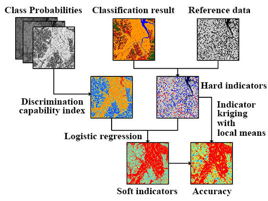
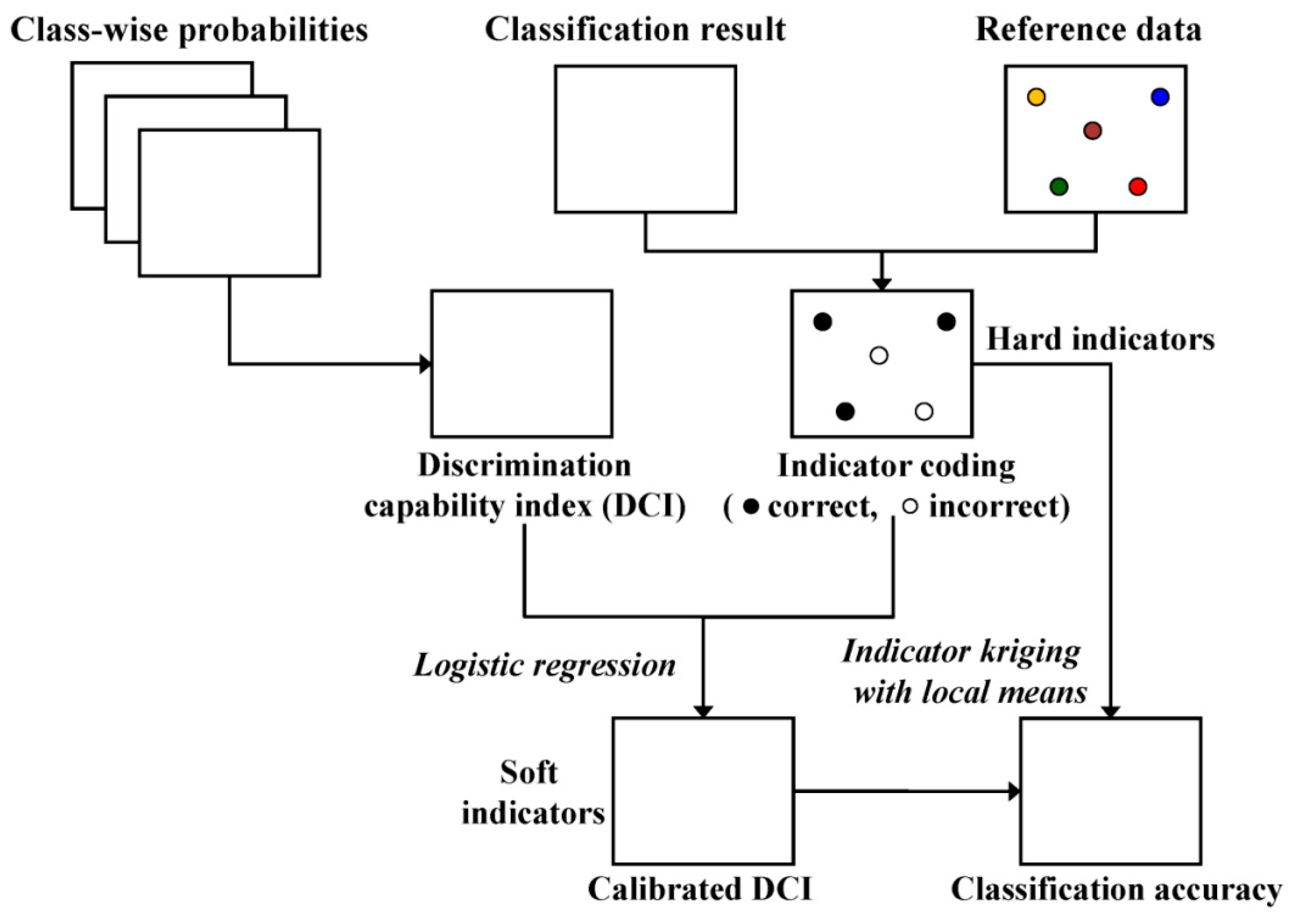
The geostatistical approach proposed in this paper for the spatial estimation of classification accuracy probability consists of three steps (Figure 2): (1) generation of class-wise probabilities for land-cover classes by applying any probabilistic classification algorithm (probabilistic classification); (2) computation of DCI values (defining ambiguity level); and (3) application of indicator kriging with local means combined with logistic regression (integration and mapping). A detailed description on each of the steps is given hereafter.

3.1. Probabilistic Classification

In the first processing step, any probabilistic algorithm capable of generating class-wise posteriori probabilities can be adopted. Bayesian probabilistic classifiers or machine learning algorithms can be applied to obtain class-wise probabilities, although some machine learning algorithms, such as support vector machines, require further post-processing to generate such posteriori probabilities. In this study, a multilayer neural network (MLP) was adopted as the main classifier, on the basis of our previous study [20].

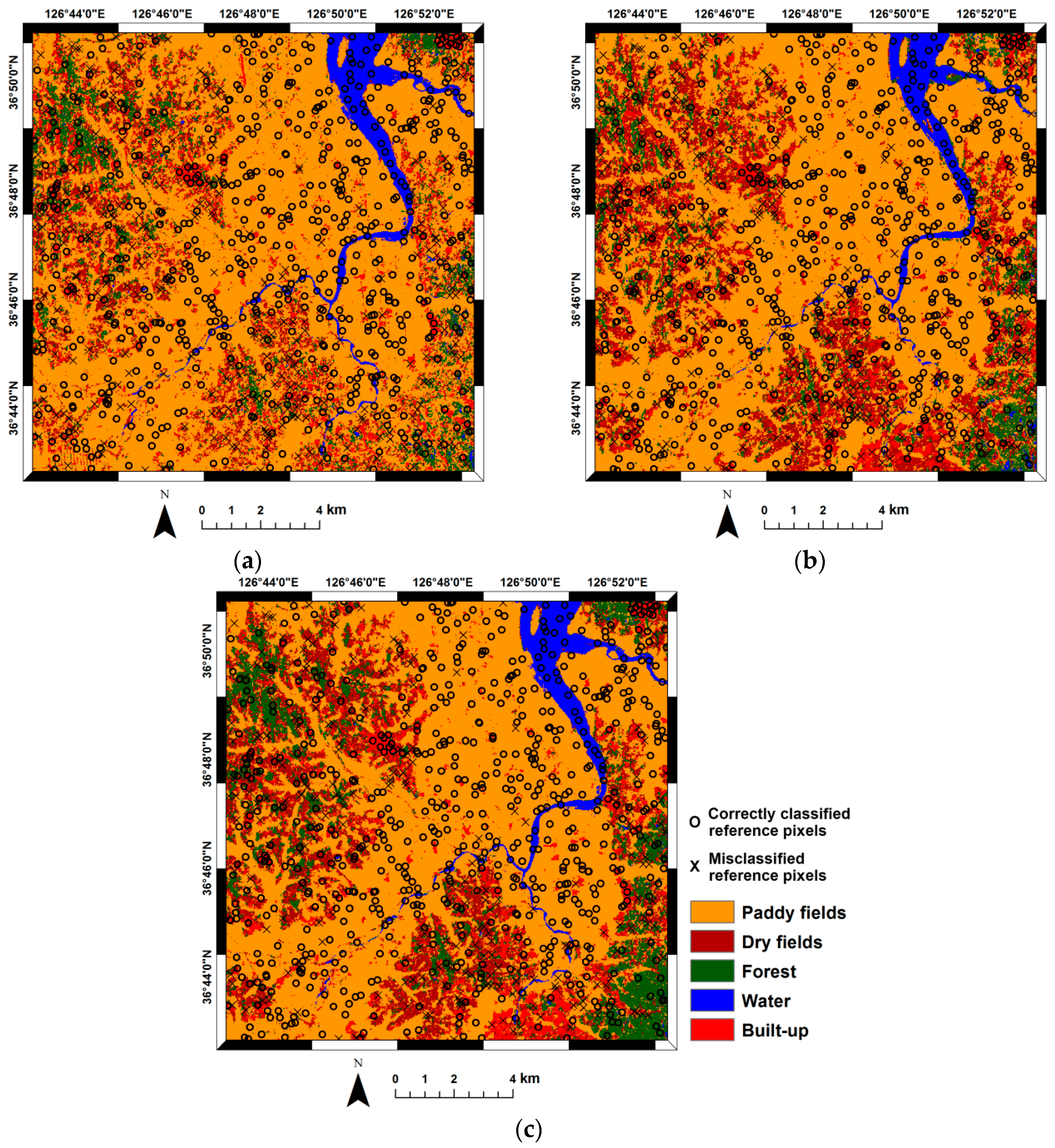
For comparison purposes, the following three classification scenarios were considered, based on: (1) Radarsat-1 features only; (2) ENVISAT ASAR features only; and (3) fusion of (1) and (2). The reason for choosing these scenarios is to highlight the effects of data fusion on classification performance by comparing the spatial distributions of classification accuracy. A concatenating fusion approach was adopted to combine the Radarsat-1 and ENVISAT ASAR features and, thereafter, the stacked multi-sensor features were used as inputs for MLP-based classification. Note that any advanced feature- or decision-level fusion technique could be applied for data fusion. However, the simple concatenating approach was selected in this study, because the main purpose here is to demonstrate the effectiveness of the proposed approach, not to select the best classifier or fusion technique.

For traditional pixel-based accuracy assessment, accuracy statistics including overall accuracy, user’s accuracy, producer’s accuracy, and the Kappa coefficient were computed from the confusion matrix. The statistical significance of the differences in classification accuracy was evaluated using the McNemar test [21].

3.2. Defining Ambiguity Level

To quantify the ambiguity in class assignment, a DCI is derived from the class-wise posteriori probabilities. In this study, the DCI is defined as the difference between the largest and the second largest posteriori probabilities as:

$$\text{DCI}\left(\mathbf{u}\right)=p\left({\omega }_{\text{max}1}\right|z\left(\mathbf{u}\right))\hspace{0.17em}-\hspace{0.17em}p({\omega }_{\text{max}2}\left|z\right(\mathbf{u}\left)\right)$$

(1)

where $\omega$ is one among the K possible land-cover classes and $z\left(\mathbf{u}\right)$ is a feature set at a certain pixel u in the study area. ${\omega }_{\text{max}1}\hspace{0.17em}=\hspace{0.17em}{\text{argmax}}_{\omega \in K}\left\{p\right(\omega \left|z\right(\mathbf{u}\left)\right)\}$ and ${\omega }_{\text{max}2}\hspace{0.17em}=\hspace{0.17em}{\text{argmax}}_{\omega \in K\backslash {\omega }_{\text{max}1}}\left\{p\right(\omega \left|z\right(\mathbf{u}\left)\right)\}$ are the most probable and the second most probable classes, respectively.

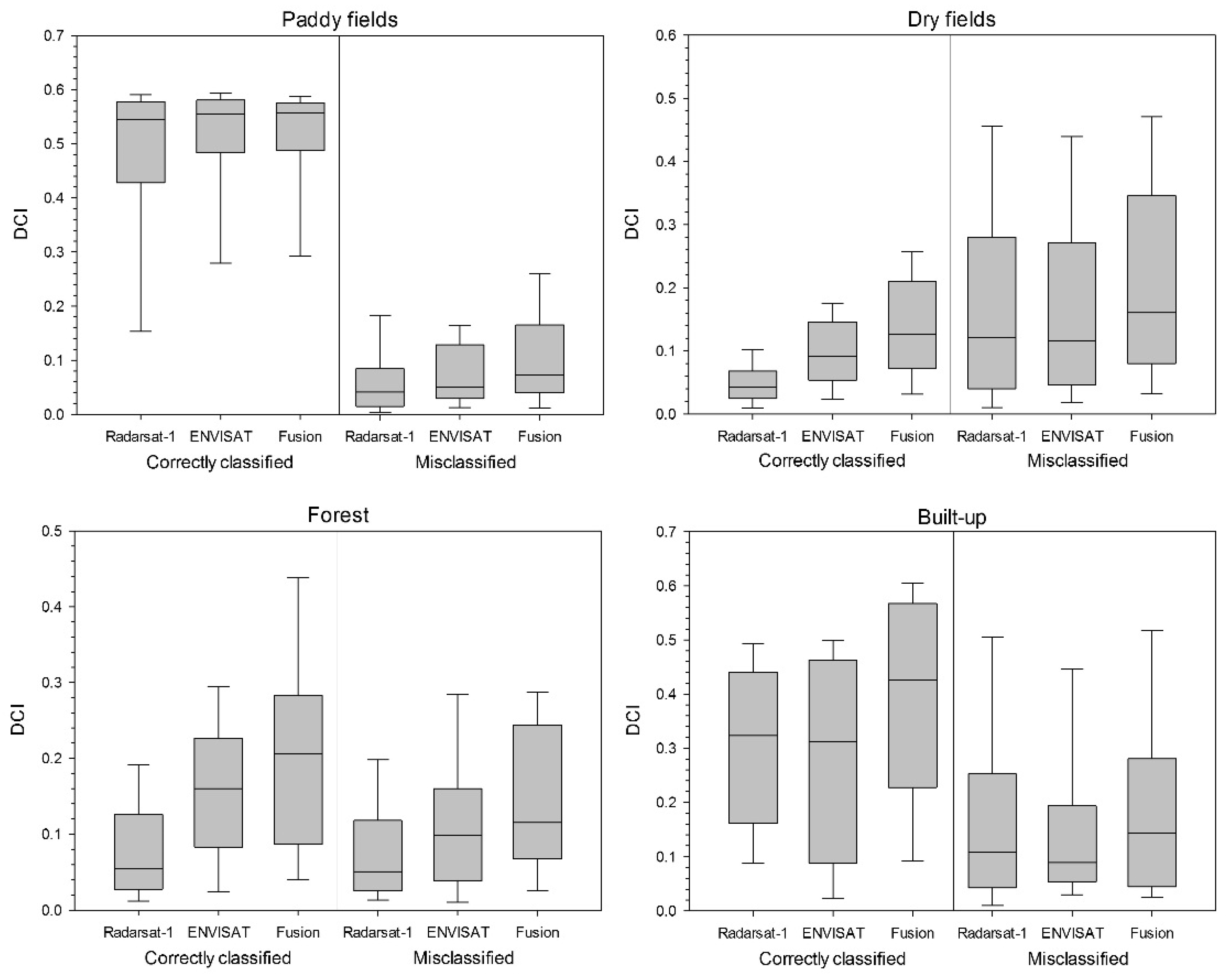
A large DCI value indicates that the class was assigned more unambiguously. The basic assumption adopted in this study is that any locations with larger DCI values are likely to have a higher accuracy level. However, the DCI provides information only on the quality of classification based on a certain input feature set and the classification algorithm used, not on the classification accuracy that can only be quantified from reference data. Therefore, another processing step is required to link the DCI values to the classification results obtained using reference data that provide actual classification accuracy (i.e., 1 or 0).

3.3. Integration and Mapping

This step involves the incorporation of classification accuracy probabilities derived at a small number of reference pixels into the image-derived exhaustive DCI values for estimating the spatial distribution of classification accuracy probabilities across the entire image.

Suppose that there are n reference pixels $\{{\mathbf{u}}_{\alpha },\hspace{0.17em}\alpha =1,\hspace{0.17em}2,\cdots ,\hspace{0.17em}n\}$ where true land-cover types are known and the DCI values are available at all pixels in the study area. The binary information on classification accuracy (correct or incorrect) at the reference pixels amounts to direct (hard) measurements of classification accuracy. Meanwhile, the DCI values provide indirect (soft) information on classification accuracy. Using both direct and indirect information, the unknown classification accuracy probabilities are estimated over the study area within an indicator framework [19]. Applications of the indicator geostatistical framework for remote sensing data classification have been previously reported in the literature [22,23,24].

The indicator approach begins with indicator coding of the available information. The binary indicators at the reference pixels ($i\left({\mathbf{u}}_{\alpha }\right)$) are defined as:

$$i({\mathbf{u}}_{\alpha })=\{\begin{array}{l}1\mathrm{correctly}\mathrm{classified}\hfill \\ 0\mathrm{misclassified}\hfill \end{array}$$

(2)

The DCI values are then calibrated or transformed into soft indicators (probabilities) to be used as local means in kriging of the above indicator-coded hard data. The soft indicator probabilities are derived from quantitative relationships between the DCI values and the hard indicator data at the reference pixels. In this study, logistic regression is adopted for calibrating the DCI values, as it is suitable for regression with a binary dependent variable [25]. In the context of this case study, the data on the dependent and independent variables are the hard indicator data and the DCI values at the reference pixels, respectively. More specifically, the calibrated DCI value at a certain pixel u in the study area (DCI_cal(u)) is defined by the following formula [25]:

$$\text{DCI\_cal}\left(\mathbf{u}\right)=1/[1+\text{Exp}[-(\mathrm{a}+\mathrm{b}\times \text{DCI}(\mathbf{u}\left)\right)]$$

(3)

where a and b are the intercept and the regression coefficient of DCI in the linear logistic model, respectively.

As logistic model predictions, the calibrated DCI values range between 0 and 1 and can, thus, be regarded as soft probabilities. Calibrated DCI values, however, need not revert to 0 or 1 at the reference pixels; hence, do not fully reproduce the corresponding hard indicator data on classification accuracy. It is, therefore, necessary to integrate both the hard indicator data and the soft DCI-derived probabilities (soft indicators) for estimating classification accuracy over the entire image.

In this work, hard and soft indicators are integrated via simple indicator kriging with local means. The constant mean in simple kriging is replaced by the soft indicators (i.e., calibrated DCI). The classification accuracy probability ($p_{acc}^{*}\left(\mathbf{u}\right)$) at an arbitrary pixel in the study area is estimated as the conditional expectation of an indicator random variable ($I\left(\mathbf{u}\right)$) from of nearby hard and soft indicator data as:

$$p_{acc}^{*}(\mathbf{u})=E\{I(\mathbf{u})|(\text{info})\}=j(\mathbf{u})+{\displaystyle \sum _{\alpha =1}^{n(\mathbf{u})}\hspace{0.17em}{\lambda }_{\alpha }(\mathbf{u})}[i({\mathbf{u}}_{\alpha })-j({\mathbf{u}}_{\alpha })]$$

(4)

where j(u) is the soft probability derived from the DCI (i.e., calibratd DCI), ${\lambda }_{\alpha }(\mathbf{u})$ is a simple kriging weight, and n(u) is the number of hard indicators within a predefined search window. The neighboring hard and soft indicators are denoted as (info).

The simple kriging weight (${\lambda }_{\alpha }\left(\mathbf{u}\right)$) is obtained by solving the following simple indicator kriging system [24]:

$${\displaystyle \sum _{\beta =1}^{n(\mathbf{u})}{\lambda }_{\beta }(\mathbf{u})C_r({\mathbf{u}}_{\alpha }-{\mathbf{u}}_{\beta })\hspace{0.17em}=}\hspace{0.17em}{C}_r({\mathbf{u}}_{\alpha }-\mathbf{u}),\forall \alpha =1,\cdots ,n(\mathbf{u})$$

(5)

where $C_r$ is the covariance function of the residuals ($r\left(\mathbf{u}\right)=i\left(\mathbf{u}\right)-j\left(\mathbf{u}\right)$).

As denoted in Equations (4) and (5), the estimate of simple indicator kriging with local means is a weighted sum of the soft indicators available at all pixels and the simple kriging estimate of residuals. By interpolating the residuals through kriging, the difference or discrepancy between hard and soft indicators can be accounted for in the classification accuracy probability estimates. The accuracy value (1 or 0) at the reference pixels is reproduced because of the exactitude property of kriging [26]. At other locations, the accuracy probability is affected by both the soft probabilities and residuals at the nearby reference pixels. As the estimation location gets farther away from the reference pixels, the impact of the soft probability becomes dominant and the estimated classification accuracy, thus, approaches to soft probability [26]. Since kriging is a non-convex interpolator [27], indicator kriging estimates that should be valued between 0 and 1 might have values less than 0 or greater than 1. These values are reset to the closest bound, 0 and 1 by adopting the common correction procedure [26,27].

4. Results and Discussion

4.1. Classification and Accuracy Assessment

MLP neural network supervised classification was employed under three scenarios, using: (1) Radarsat-1 features only; (2) ENVISAT ASAR features only; and (3) fusion of (1) and (2). For each scenarios, the MLP neural network consists of an input layer with neurons corresponding to the size of the features, one hidden layer, and an output layer with five neurons. The optimal number of neurons in the hidden layer was selected through four-fold cross validation and the conjugate gradient algorithm was used to train the network. The DTREG software [28] was used to implement MLP neural network supervised classification.

Once the posteriori probability for each class was obtained, the classification result was generated by applying a maximum a posteriori decision rule (Figure 3). From the visual inspection, paddy fields in the central region and water are well identified in all classification scenarios. However, the three classification scenarios, except for these two classes, showed different classification results, particularly in the northwestern region of the study area. In that region, more fragmented classification patterns and decreased dry fields are observed in the classification result using Radarsat-1 features (Figure 3a), in comparison to other classification results. Meanwhile, the respective increase and decrease of forest and dry fields in that region are shown in the classification result using ENVISAT ASAR features (Figure 3b). The fusion of all features from each sensor displays mixed patterns of above two classification results from both sensors, particularly more clustered dry fields and forest classes (Figure 3c). In addition, most pixels in the bottom right corner of the study area were classified as forest, unlike the classification result from each single sensor. These different classification results indicate the different classification performance or accuracy between the three classification scenarios.

The confusion matrices with related accuracy statistics for the three classification scenarios are listed in

Table 3. Confusion matrix and accuracy statistics for classification using Radarsat-1 features.

	Reference	Paddy Fields	Dry Fields	Forest	Water	Built-up	User’s Accuracy
Classification
Paddy fields		445	84	30	5	38	73.92%
Dry fields		22	51	17	1	9	51.00%
Forest		11	11	32	0	9	50.79%
Water		2	2	1	47	0	90.38%
Built-up		9	6	11	0	63	70.79%
Producer’s accuracy		91.00%	33.12%	35.16%	88.68%	52.94%
Overall accuracy: 70.42%
Kappa coefficient: 0.51

,

Table 4. Confusion matrix and accuracy statistics for classification using ENVISAT ASAR features.

	Reference	Paddy Fields	Dry Fields	Forest	Water	Built-up	User’s Accuracy
Classification
Paddy fields		443	61	19	8	35	78.27%
Dry fields		31	71	36	3	46	37.97%
Forest		8	18	33	2	8	47.83%
Water		2	0	1	40	0	93.02%
Built-up		5	4	2	0	30	73.17%
Producer’s accuracy		90.59%	46.10%	36.26%	75.47%	25.21%
Overall accuracy: 68.10%
Kappa coefficient: 0.48

and

Table 5. Confusion matrix and accuracy statistics for classification using fusion of all features.

	Reference	Paddy Fields	Dry Fields	Forest	Water	Built-up	User’s Accuracy
Classification
Paddy fields		445	49	7	3	21	84.76%
Dry fields		25	79	22	3	20	53.02%
Forest		8	22	61	0	14	58.10%
Water		1	0	0	47	0	97.92%
Built-up		10	4	1	0	64	81.01%
Producer’s accuracy		91.00%	51.30%	67.03%	88.68%	53.78%
Overall accuracy: 76.82%
Kappa coefficient: 0.63

. When comparing the accuracy statistics of each single sensor feature set, the overall accuracy and Kappa coefficient based on the Radarsat-1 features were slightly higher than those of using ENVISAT ASAR features. However, the McNemar test revealed that the difference in the overall accuracy between these two classification results is not statistically significant at the 5% significance level. The fusion of multi-sensor features showed the best accuracy statistics. Increases of about 6.4 and 8.7 percentage points in overall accuracy were achieved, compared with the classification results from Radarsat-1 and ENVISAT ASAR features, respectively. These differences in the classification accuracy are statistically significant at the 5% significance level.

The different classification accuracies between the three classification scenarios were further highlighted by comparing class-wise accuracy statistics. As expected from the visual inspection of the classification results shown in Figure 3, the accuracies of dry fields and forest are relatively low. In the classification using Radarsast-1 features, most of the dry fields and forest were misclassified as paddy fields and exaggerated paddy fields thus exist in the northwestern region, as shown in Figure 3a. Using ENVISAT ASAR features also yields misclassification of dry fields and forest. In particular, the forest class was misclassified mainly as dry fields, which results in the decreased forest in the northwestern region of Figure 3b. It is noteworthy that most built-up reference pixels were misclassified as paddy fields and dry fields, showing the lowest producer’s accuracy. The built-up areas typically exhibit high backscattering coefficients, but the backscattering signatures depend on the orientation and density of structures. The study area is a rural area that consists mainly of low-rise houses and structures with low density. The backscattering signatures from VV polarization with the steep incidence angle may have a wide range in some of the built-up areas and, thus, overlap with those of other classes. The fusion of all features leads to the improvement in the accuracy statistics in all classes. Although dry fields and forest still have relatively lower classification accuracies than those of other classes, confusion between these classes is reduced. In particular, the contribution of a combination of multiple polarization features is significant in forest.

4.2. Classificaion Ambiguity Analysis

As a quantitative measure of classification ambiguity, the DCI was computed from class-wise posteriori probabilities using Equation (1). As shown in Figure 4, the highest DCI values are observed in both paddy fields and water, regardless of the classification scenario. Relatively low DCI values in all classification scenarios are observed in other regions classified as dry fields and forest, indicating the high ambiguity or uncertainty in class assignment of these classes. The fusion of all features showed a slight increase of the mean of DCI values at all pixels (0.36), in comparison to those of Radarsat-1 and ENVISAT features (0.32 and 0.34, respectively).

To investigate the relationships between DCI values and the classification results at reference pixels, summary statistics of the DCI values at correctly and incorrectly classified reference pixels were computed and are listed in

Table 6. Summary statistics of DCI values at the correctly and incorrectly classified reference pixels for different classification scenarios.

Class	Data	Mean	Std. dev.	Lower Quartile	Median	Upper Quartile
Correctly classified	Radarsat-1	0.405	0.205	0.214	0.512	0.569
	ENVISAT ASAR	0.424	0.197	0.269	0.530	0.578
	Fusion	0.424	0.189	0.269	0.533	0.573
Misclassified	Radarsat-1	0.137	0.153	0.030	0.077	0.176
	ENVISAT ASAR	0.146	0.146	0.043	0.093	0.185
	Fusion	0.185	0.157	0.058	0.136	0.281

. The overall DCI values at the correctly classified reference pixels are much greater than those at the misclassified reference pixels, regardless of the classification scenario. This distinctive difference in the distributions of the DCI values between correct and incorrect classification implies that the DCI can be used as a good discrimination index in class assignment and, thus, used as indirect information on classification accuracy at areas where true land-cover types are not available.

However, the paddy fields class, which is a major land-cover type in the study area (about 54% in reference data) and was also classified correctly for the most part, may affect the distribution of DCI values at the correctly classified reference pixels. To further investigate this issue, the distributions of the DCI values for each class were also generated (Figure 5). The water class was excluded from the analysis because its small number of misclassified reference pixels was not suitable for statistical analysis. As expected, the distributions of the DCI values between the correctly and incorrectly classified reference pixels are well separated in paddy fields. Despite some overlap between the distributions, the built-up class also exhibits distinct differences. The fusion of all features shows an increase in the DCI values at correctly classified reference pixels, which indicates that complimentary information could be obtained from the fusion of multiple polarization features resulting into improved classification accuracy. On the contrary, DCI values for dry fields and forest, classes exhibiting relatively low classification accuracies, show significant overlapping distributions at both correctly and incorrectly classified reference pixels, unlike paddy fields and built-up. Much greater variance and range values are also observed in the distributions of DCI values at misclassified reference pixels, regardless of the classification scenario. In particular, using Radarsat-1 features results in much smaller DCI values at correctly classified dry fields pixels than at misclassified dry fields pixels. This poor distinction of dry fields and forest indicates that some pixels of those two classes were confidently assigned to the incorrect class due to the lack of proper information from input features. This result implies that such discrepancies between the DCI values and the classification accuracy at the reference pixels should be calibrated or accounted for when used as indirect soft information for the estimation of the spatial distribution of classification accuracy.

4.3. Spatial Estimation of Classification Accuracy

4.3.1. Logistic Regression

Once the DCI values for all classification scenarios were prepared, they were calibrated via logistic regression with indicator-coded reference data. By definition, the mean of the calibrated DCI values corresponds to the proportion of correctly classified reference pixels (i.e., overall accuracy), while the residuals, which are the differences between the hard indicators and the logistic model predictions, have a zero mean. The overall fit of logistic regression was quantified using the Nagelkerke R-squared, with values of 0.364, 0.419, and 0.370 for Radarsat-1, ENVISAT ASAR, and fusion, respectively. To consider the different distributions of DCI values at the correctly and incorrectly classified reference pixels in Figure 5, the land-cover classification results at reference pixels were used as data on another independent variable in logistic regression. By including land-cover classes at reference pixels with DCI values, the Nagelkerke R-squared values increased, i.e., 0.397, 0.430, and 0.377 for Radarsat-1, ENVISAT ASAR, and fusion, respectively. However, not all logistic regression coefficients were statistically significant at the 5% significance level. For example, when both DCI and land-cover classes were used for logistic regression modeling of the Radarsat-1 dataset and the reference class for categorical land-cover classes was set to water, only DCI was statistically significant at the 5% significance level. Even though slightly lower R-squared values are obtained from logistic regression using only the DCI values, the variability unexplained by logistic regression is included in the residuals and could affect the estimation of classification accuracy via kriging of the residuals. Thus, land-cover classes were not used as additional independent variables for logistic regression. However, the use of other variables, such as the dimension of land-cover patches and the proximity to the border, may affect logistic regression modeling. The effects of those variables should be further investigated in future research.

Figure 6 presents the distributions of residuals at the reference pixels. The positive and negative residuals, which are associated with correctly and incorrectly classified reference pixels, respectively, are separated reasonably well for all classification scenarios. The relatively large residuals of misclassified hard data indicate that the logistic model fits better to the correctly classified hard data than the misclassified hard data with much greater variance and a wide range of DCI values. Since the residuals that were not accounted for by the DCI could not be ignored, they were incorporated into the estimation of the accuracy probability.

4.3.2. Integration and Mapping

To estimate residuals at any pixel in the study area, experimental variograms were first computed and fitted visually. The variogram model type and its associated parameters are given in

Table 7. Model type and associated parameters for the variogram of residuals.

Data	Model Type	Nugget Effect	Partial Sill	Range (m)
Radarsat-1	Spherical	0.11	0.03	830
ENVISAT ASAR	Spherical	0.10	0.04	614
Fusion	Spherical	0.07	0.06	614

. After variogram modeling of residuals, the residuals were estimated over the entire image using simple kriging and the variogarm model of the residuals. The estimated residuals were then added to the calibrated DCI values to obtain the final accuracy probability values at all pixels in the study area.

Figure 7 presents three classification accuacy probability maps obtained using simple indicator kriging with local means. The bull’s eye effects around misclassified reference pixels are mainly due to the short range structure of the variogram model of residuals. The mean of all accuracy probability values in the study area corresponds to overall accuracy; in other words, locally varying degrees of accuracy can be estimated while maintaining the overall global accuracy statistics corresponding to the reference data. The distributions of the accuracy probability for each class of the different classification scenarios are also presented in Figure 8. From Figure 7 and Figure 8, paddy fields and water showed the largest accuracy probability in all classification scenarios. The fusion of all features resulted in an increase in the accuracy probability in other classes that showed relatively low classification accuracy when features from a single sensor were used for classification; this result confirms the benefit of data fusion for land-cover classification.

The difference maps between the classification scenarios were also generated to identify the area where a significant increase in the accuracy probability was obtained by data fusion (Figure 9). The effects of data fusion are well presented in the areas classified as dry fields and forest (red color in Figure 9). In particular, an increase in the accuracy probability was observed in some built-up areas at the center of the study area that were misclassified as other classes in the classfication using ENVISAT ASAR features (Figure 9b). Despite an overall improvement in accuracy estimation by data fusion, there are still some areas exhibiting a decrease in the accuracy probability (blue color in Figure 9). These areas are mainly located near the misclassfied reference data, but were correctly classified when using features from a single sensor. Some paddy fields also showed a slight decrease in accuracy probability values for the data fusion scenario. These results indicate that the fusion of features from multiple polarization data did not always lead to an improvement in the classfication accuracy at all locations. Therefore, a detailed ground survey or an investigation of the intrinsic characteristics of input features and/or the MLP classifier may be required in those regions. The low classification accuracy in dry fields and forest implies a necessity to use other features that were not considered for the current classification, but can provide more discriminative information to improve the classification accuracy for those classes. In this type of further investigation, the spatial distribution of classification accuracy can still be a primary information source.

5. Conclusions

An indicator geostatistical approach incorporating quantitative ambiguity measures derived from probabilistic classifiers was presented in this study to estimate the spatial distribution of classification accuracy. Unlike traditional accuracy statistics from a confusion matrix, the proposed approach can furnish classification accuracy probability values in areas where true land-cover types are not available and, hence, provide a useful source of information for assessing map quality and guiding additional ground surveys. A case study using multi-temporal and multi-sensor SAR datasets for land-cover classification demonstrated the applicability of the presented approach, while also highlighting the benefit of data fusion.

From a methodological viewpoint, the main novelty of the proposed approach lies in the derivation and integration of the DCI that provides indirect information about varying degrees of classification ambiguity or uncertainty. Logistic regression and interpolation of residuals are also combined to calibrate the DCI so as to reflect the actual classification results (correct or incorrect classification) at a small number of reference pixels, respectively. Through this integration approach, overall accuracy from a confusion matrix can be still estimated while also providing per pixel accuracy probability values. The simplicity of the integration procedure via indicator kriging with local means is other advantage of the proposed approach. If data on other indirect information are available, logistic regression can be easily applied to the entire set of indirect information and only one variogram model for the residuals is required, unlike co-kriging that calls for time-consuming variogram modeling.

The output of the indicator approach in this study provides estimated classification accuracy probability values quantifying the degree of correct classification for all land-cover classes. In practice, however, this probability may not be sufficient for the investigation of the misclassification characteristics of a certain class of interest. For example, one may be interested in the misclassification probability of dry fields into forest or paddy fields. To derive this kind of information, another source, for example, the user’s accuracy from the confusion matrix, should be defined and integrated. Future research along these lines is required to extend the proposed approach for furnishing additional interpretable probabilistic products.

References

1. Lee, S. Application of logistic regression model and its validation for landslide susceptibility mapping using GIS and remote sensing. Int. J. Remote Sens. 2005, 26, 1477–1491. [Google Scholar] [CrossRef]
2. Doraiswamy, P.C.; Sinclair, T.R.; Hollinger, S.; Akhmedov, B.; Stern, A.; Prueger, J. Application of MODIS derived parameters for regional crop yield assessment. Remote Sens. Environ. 2005, 97, 192–202. [Google Scholar] [CrossRef]
3. Hoek, G.; Beelen, R.; de Hoogh, K.; Vienneau, D.; Gulliver, J.; Fischer, P.; Briggs, D. A review of land-use regression models to assess spatial variation of outdoor air pollution. Atmos. Environ. 2008, 42, 7561–7578. [Google Scholar] [CrossRef]
4. Heuvelink, G.B.M. Error Propagation in Environmental Modeling with GIS; Taylor & Francis: London, UK, 1998. [Google Scholar]
5. Solaiman, B.; Pierce, L.E.; Ulaby, F.T. Multisensor data fusion using fuzzy concepts: Application to land-cover classification using ERS-1/JERS-1 SAR composites. IEEE Trans. Geosci. Remote Sens. 1999, 37, 1316–1326. [Google Scholar] [CrossRef]
6. Bruzzone, L.; Prieto, D.F.; Serpico, S.B. A neural-statistical approach to multitemporal and multisource remote-sensing image classification. IEEE Trans. Geosci. Remote Sens. 1999, 37, 1350–1359. [Google Scholar] [CrossRef]
7. Briem, G.J.; Benediktsson, J.A.; Sveinsson, J.R. Multiple classifiers applied to multisource remote sensing data. IEEE Trans. Geosci. Remote Sens. 2002, 40, 2291–2299. [Google Scholar] [CrossRef]
8. Gislason, P.O.; Benediktsson, J.A.; Sveinsson, J.A. Random forests for land cover classification. Pattern Recogn. Lett. 2006, 27, 294–300. [Google Scholar] [CrossRef]
9. Waske, B.; Benediktsson, J.A. Fusion of support vector machines for classification of multisensory data. IEEE Trans. Geosci. Remote Sens. 2007, 45, 3858–3866. [Google Scholar] [CrossRef]
10. Gong, B.; Im, J.; Mountrakis, G. An artificial immune network approach to multi-sensor land use/cover classification. Remote Sens. Environ. 2011, 115, 600–614. [Google Scholar] [CrossRef]
11. Moser, G.; Serpico, S.B. Combining support vector machines and Markov random fields in an integrated framework for contextual image classification. IEEE Trans. Geosci. Remote Sens. 2013, 51, 2734–2752. [Google Scholar] [CrossRef]
12. Chen, C.; Li, W.; Su, H.; Liu, K. Spectral-spatial classification of hyperspectral image based on kernel extreme learning machine. Remote Sens. 2014, 6, 5795–5814. [Google Scholar] [CrossRef]
13. Liu, X.; Bo, Y. Object-based crop species classification based on the combination of airborne hyperspectral images and LiDAR data. Remote Sens. 2015, 7, 922–950. [Google Scholar] [CrossRef]
14. Lillesand, T.; Kiefer, R.W.; Chipman, J. Remote Sensing and Image Interpretation, 6th ed.; Wiley: New York, NY, USA, 2007. [Google Scholar]
15. Congalton, R.G.; Green, K. Assessing the Accuracy of Remotely Sensed Data: Principles and Practices, 2nd ed.; CRC Press: New York, NY, USA, 2008. [Google Scholar]
16. Zhu, A.X. Measuring uncertainty in class assignment for natural resource maps under fuzzy logic. Photogramm. Eng. Remote Sens. 1997, 63, 1195–1202. [Google Scholar]
17. Steele, B.M.; Winne, J.C.; Redmond, R.L. Estimation and mapping of misclassification probabilities for thematic land cover mapping. Remote Sens. Environ. 1998, 66, 192–202. [Google Scholar] [CrossRef]
18. Kyriakidis, P.C.; Dungan, J.L. A geostatistical approach for mapping thematic classification accuracy and evaluating the impact of inaccurate spatial data on ecological model predictions. Environ. Ecol. Stat. 2001, 8, 311–330. [Google Scholar] [CrossRef]
19. Journel, A.G. Non-parametric estimation of spatial distribution. Math. Geol. 1983, 15, 445–468. [Google Scholar] [CrossRef]
20. Park, N.-W.; Chi, K.-H. Integration of multitemporal/polarization C-band SAR data sets for land-cover classification. Int. J. Remote Sens. 2008, 29, 4667–4688. [Google Scholar] [CrossRef]
21. Foody, G.M. Thematic map comparison: Evaluating the statistical significance of differences in classification accuracy. Photogramm. Eng. Remote Sens. 2004, 70, 627–633. [Google Scholar] [CrossRef]
22. Van der Meer, F. Classification of remotely-sensed imagery using an indicator kriging approach: Application to the problem of calcite-dolomite mineral mapping. Int. J. Remote Sens. 1996, 17, 1233–1249. [Google Scholar] [CrossRef]
23. Goovaerts, P. Geostatistical incorporation of spatial corrdinates into supervised classification of hyperspectral data. J. Geograph. Syst. 2002, 4, 99–111. [Google Scholar] [CrossRef]
24. Chiang, J.-L.; Liou, J.-J.; Wei, C.; Cheng, K.-S. A feature-space indicator kriging approach for remote sensing image classification. IEEE Trans. Geosci. Remote Sens. 2014, 52, 4046–4055. [Google Scholar] [CrossRef]
25. Hilbe, J.M. Logistic Regression Models; CRC Press: New York, NY, USA, 2009. [Google Scholar]
26. Goovaerts, P. Geostatistics for Natural Resources Evaluation; Oxford University Press: New York, NY, USA, 1997. [Google Scholar]
27. Deutsch, C.V.; Journel, A.G. GSLIB: Geostatistical Software Library and User’s Guide, 2nd ed.; Oxford University Press: New York, NY, USA, 1998. [Google Scholar]
28. Sherrod, P.H. DTREG Predictive Modeling Software. Available online: http://www.dtreg.com (accessed on 25 November 2015).
Figure 1. Location of the study area and the Radarsat-1 average backscattering coefficient image with training data (red dots) and reference data (blue dots).
Remotesensing 08 00320 g001
Figure 2. Flowchart of the processing steps presented in this study.
Remotesensing 08 00320 g002
Figure 3. Classification maps with classification results at reference pixels: (a) Radarsat-1; (b) ENVISAT ASAR; and (c) fusion.
Remotesensing 08 00320 g003
Figure 4. DCI maps: (a) Radarsat-1; (b) ENVISAT ASAR; and (c) fusion.
Remotesensing 08 00320 g004
Figure 5. Box plot of DCI values per each class at the correctly and incorrectly classified reference pixels for different classification scenarios. For each box plot, whiskers above and below the box indicate the 90th and 10th percentiles, respectively. The top and bottom boundaries of the box indicate upper and lower quartiles, respectively. The line within the box corresponds to the median.
Remotesensing 08 00320 g005
Figure 6. Box plots of residuals at correctly and incorrectly classified reference pixels.
Remotesensing 08 00320 g006
Figure 7. Classification accuracy probability maps: (a) Radarsat-1; (b) ENVISAT ASAR; and (c) fusion.
Remotesensing 08 00320 g007
Figure 8. Box plots of accuracy probability values per class for different classification scenarios. R, E, and F on the x-axis stand for Radarsat-1, ENVISAT ASAR, and fusion, respectively. Numbers next to abbreviations indicate class codes (1: paddy fields, 2: dry fields, 3: forest, 4: water, 5: built-up).
Remotesensing 08 00320 g008
Figure 9. Difference maps of estimated classification accuracy probability: (a) fusion-Radsarsat-1; and (b) fusion-ENVISAT ASAR.
Remotesensing 08 00320 g009