
Scaling of FAPAR from the Field to the Satellite


Abstract
:
1. Introduction
2. Study Area and Data
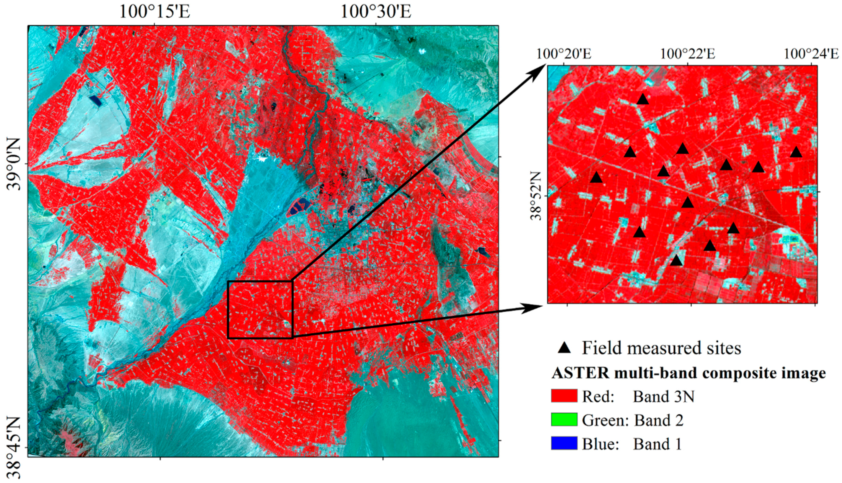
2.1. Study Area
2.2. Measurement and Data Preparation
2.2.1. In-situ Measurement
2.2.2. Satellite Data and Preprocessing
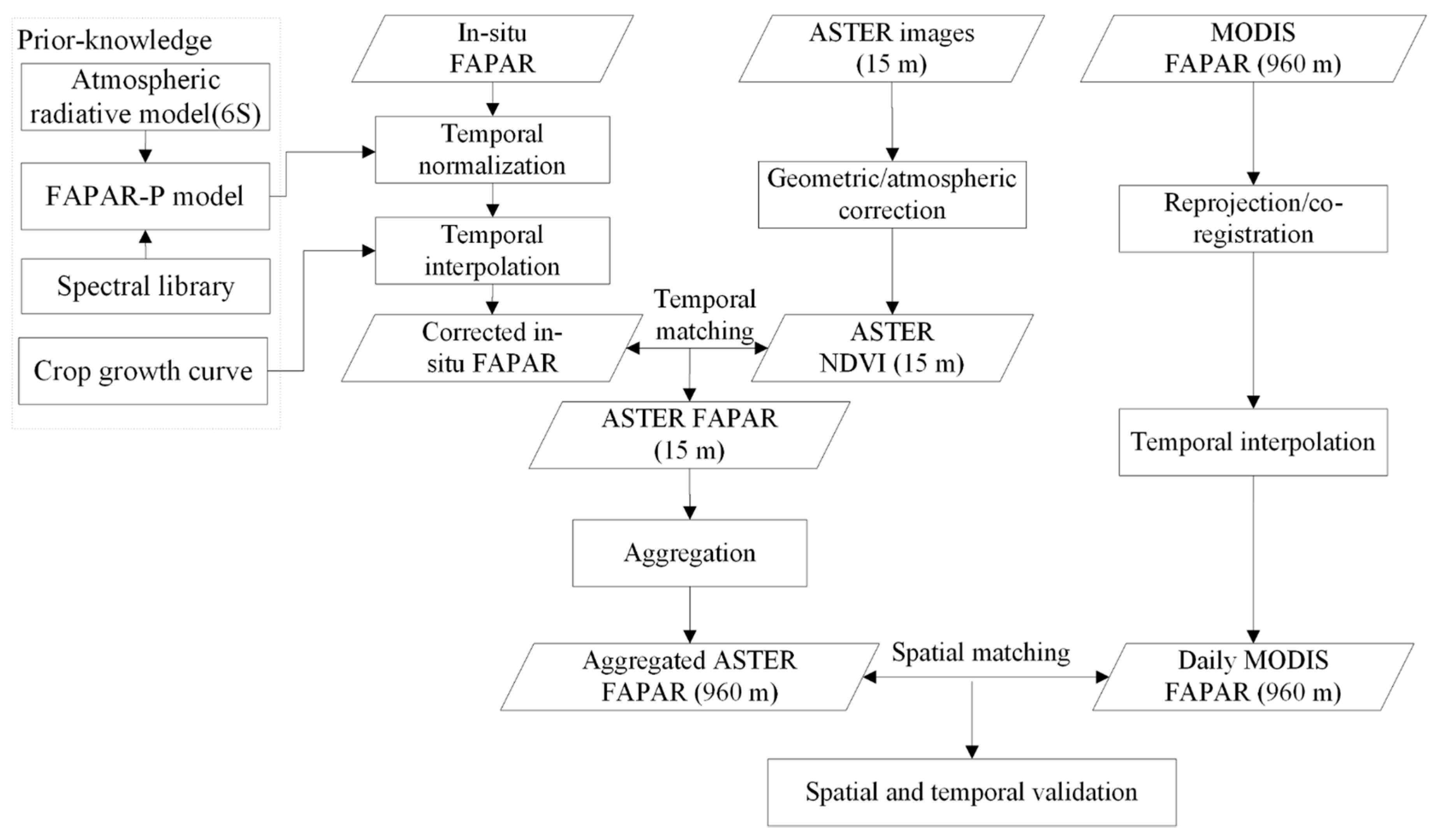
3. Methodology
3.1. FAPAR Definition
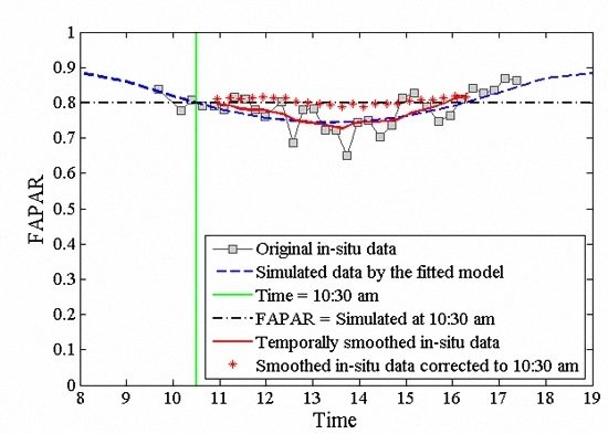
3.2. Temporal Normalization
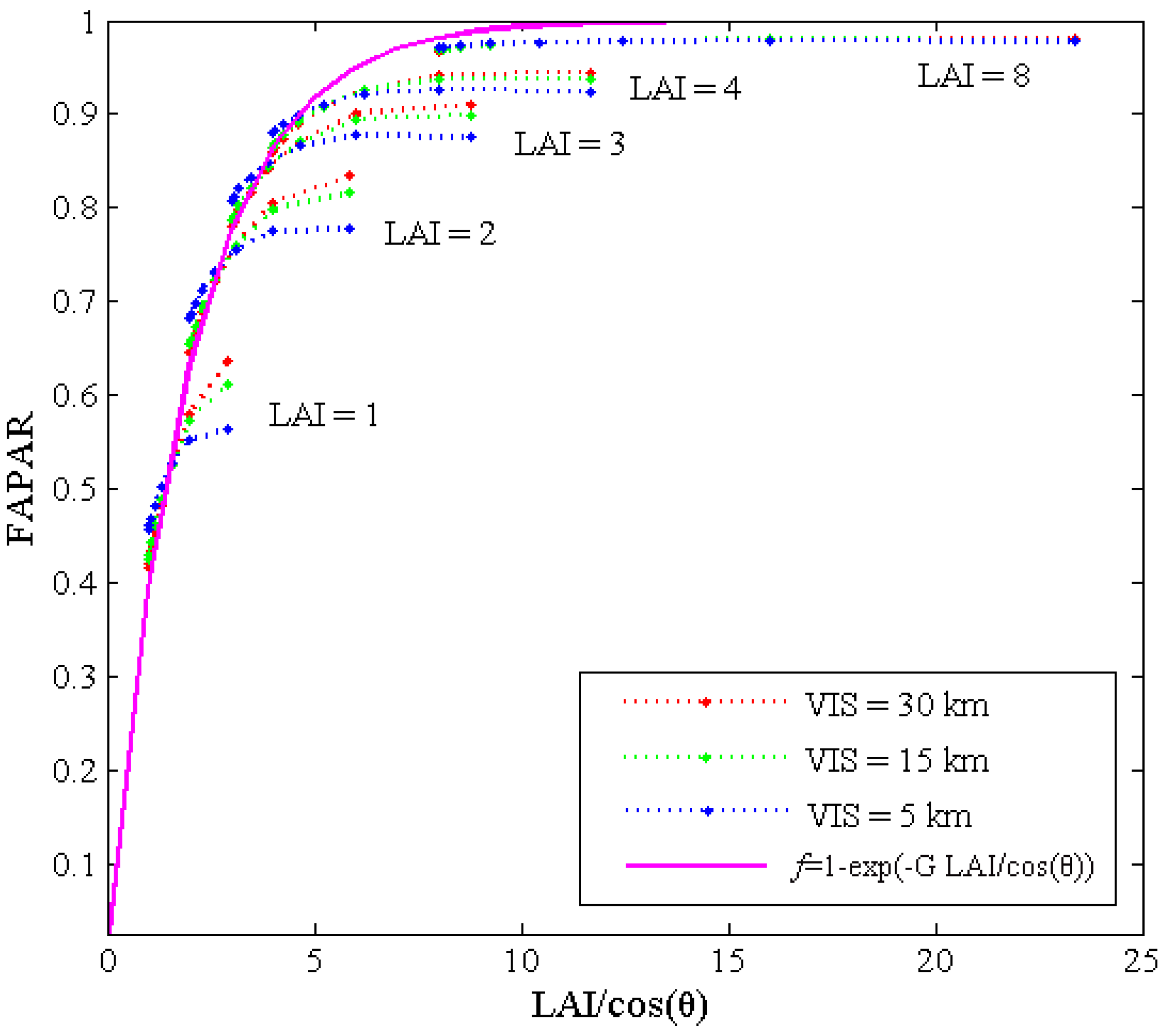
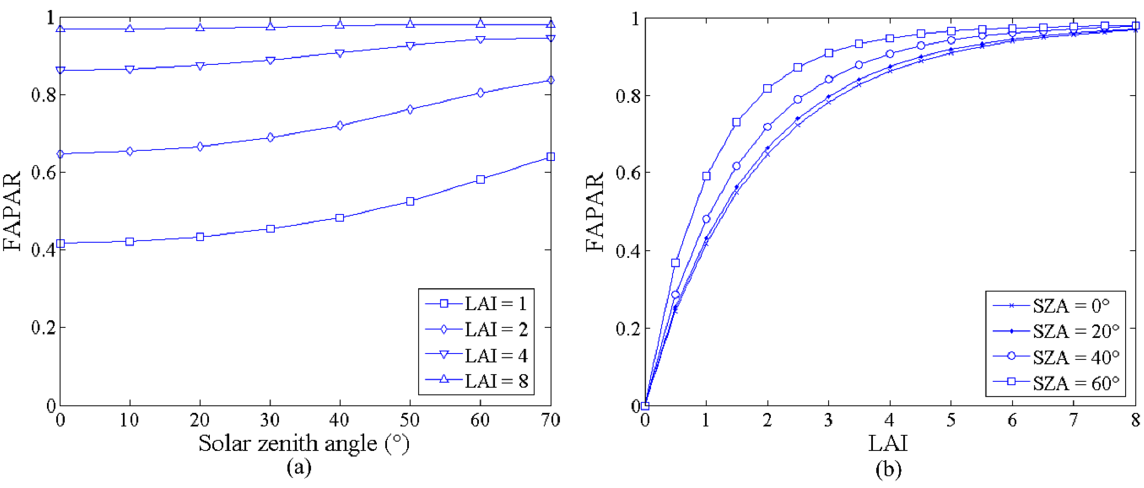
3.2.1. FAPAR-P Model
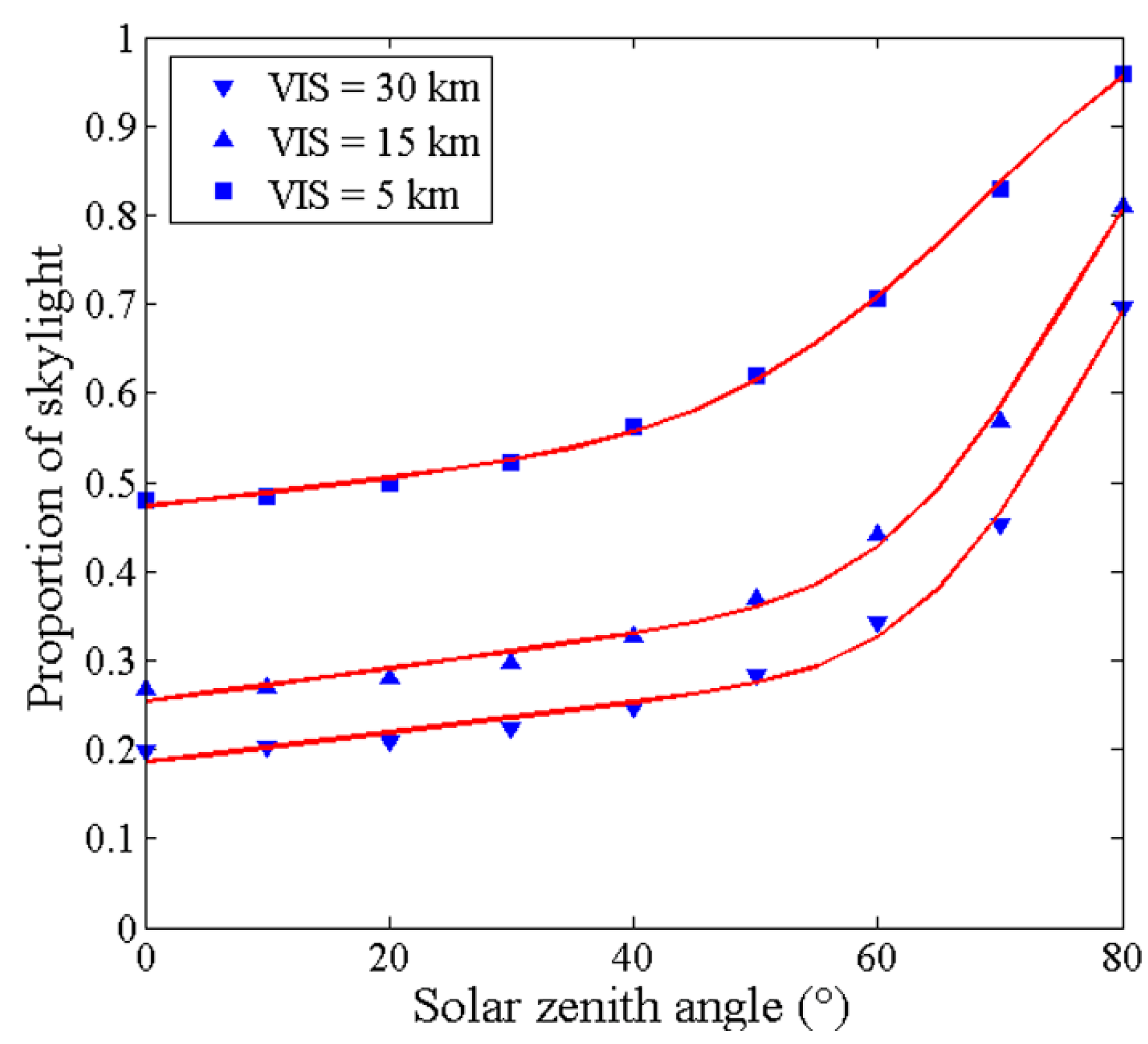
3.2.2. Estimation of Skylight Proportion
3.2.3. FAPAR Model Integrating FAPAR-P and 6S Models
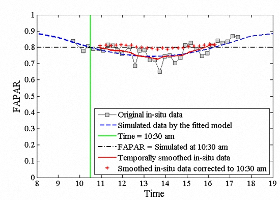
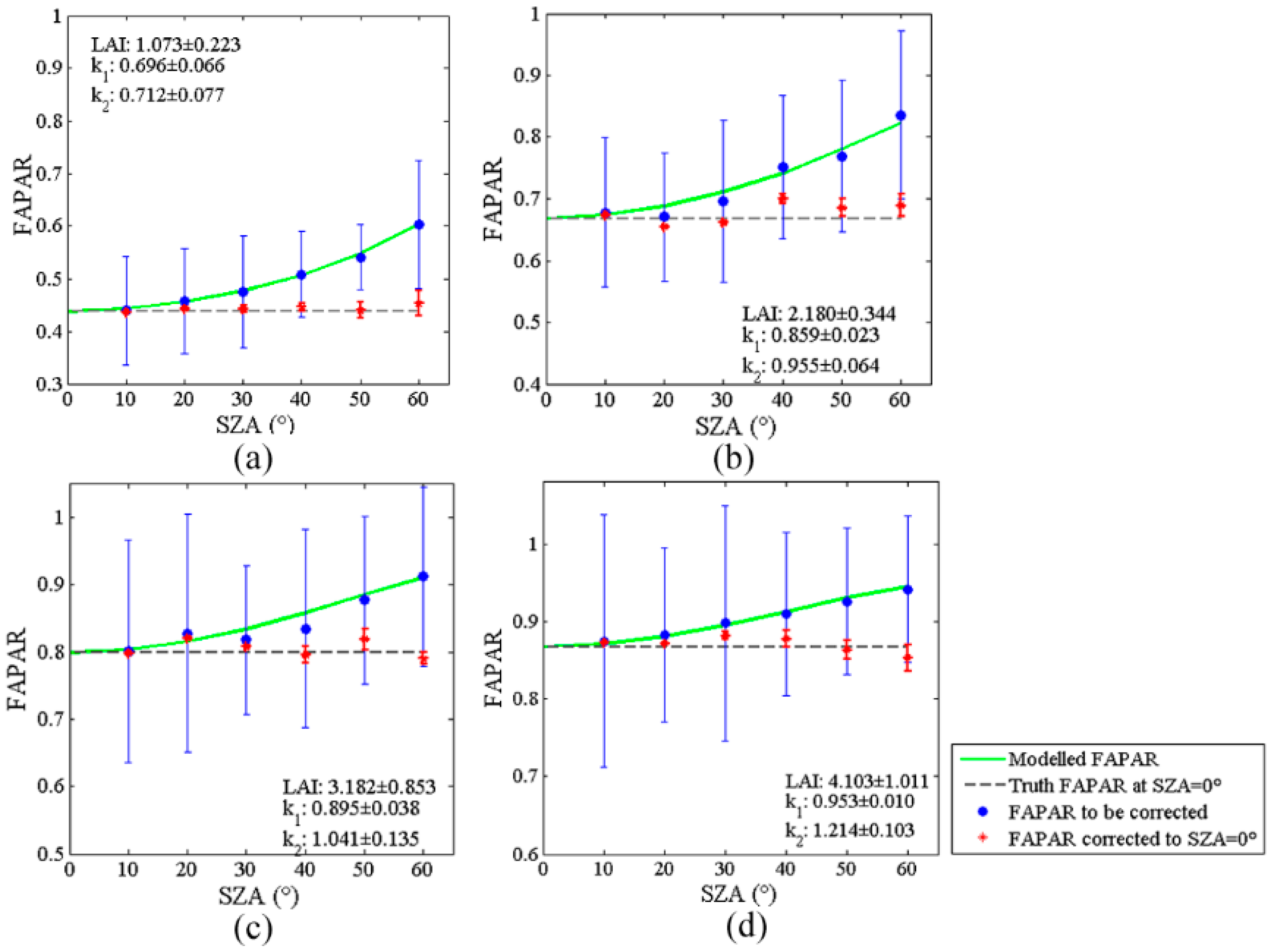
3.2.4. Simplified SZA Correction Model
3.3. Temporal Interpolation
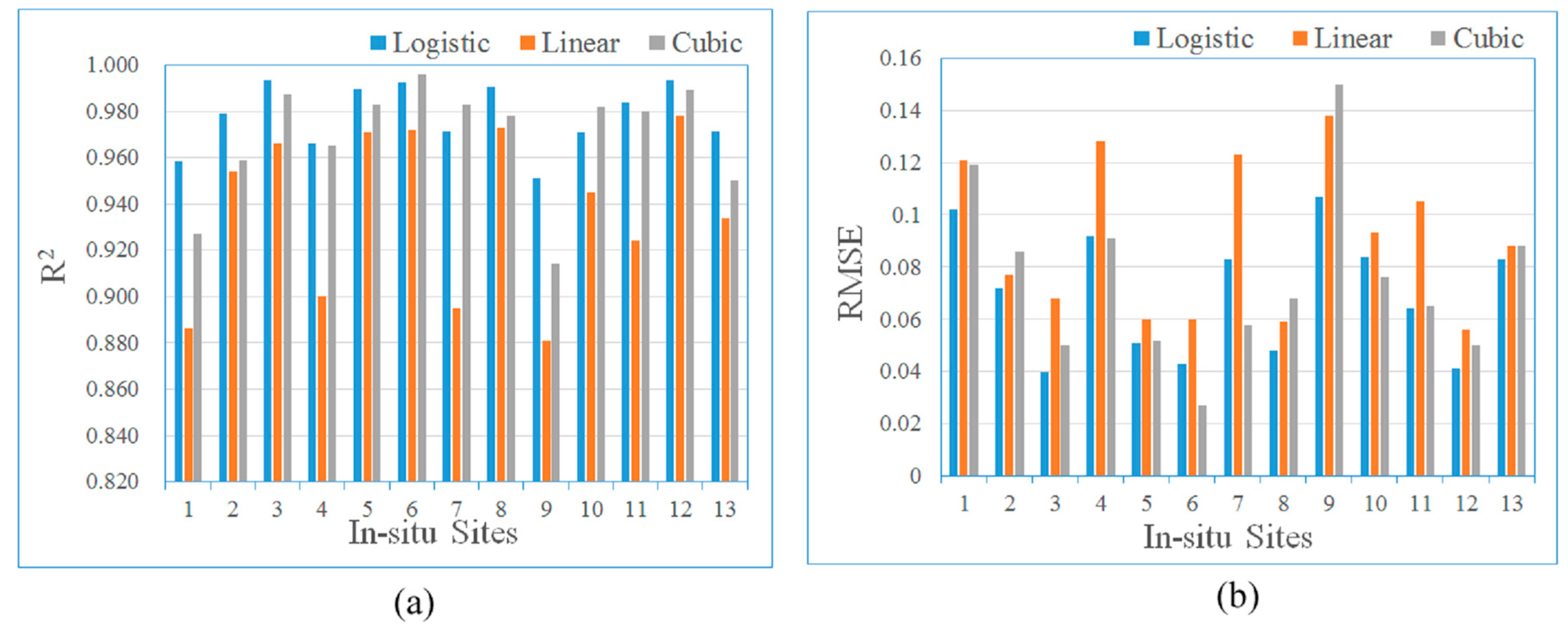
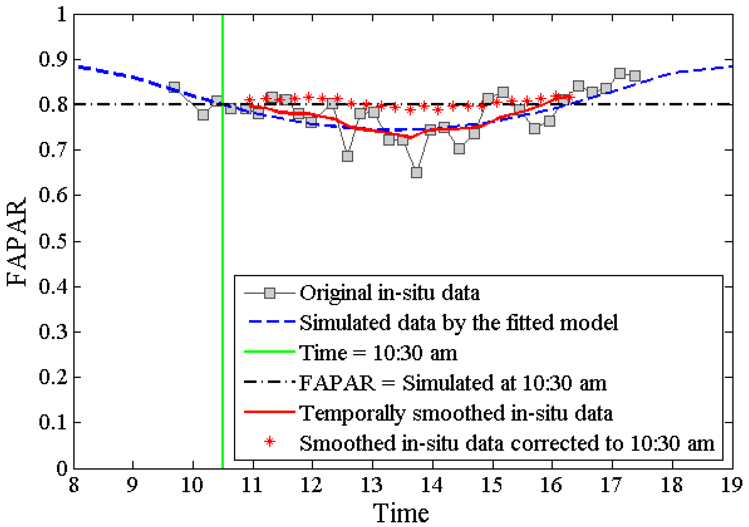
3.3.1. Interpolating in-Situ Measurements to ASTER Dates
3.3.2. Interpolating MODIS FAPAR to ASTER Dates
3.4. Multi-Scale FAPAR Truth Data
3.4.1. Estimating Fine-Resolution FAPAR
3.4.2. Coarse-Resolution FAPAR
4. Results and Analysis
4.1. Temporal Corrections
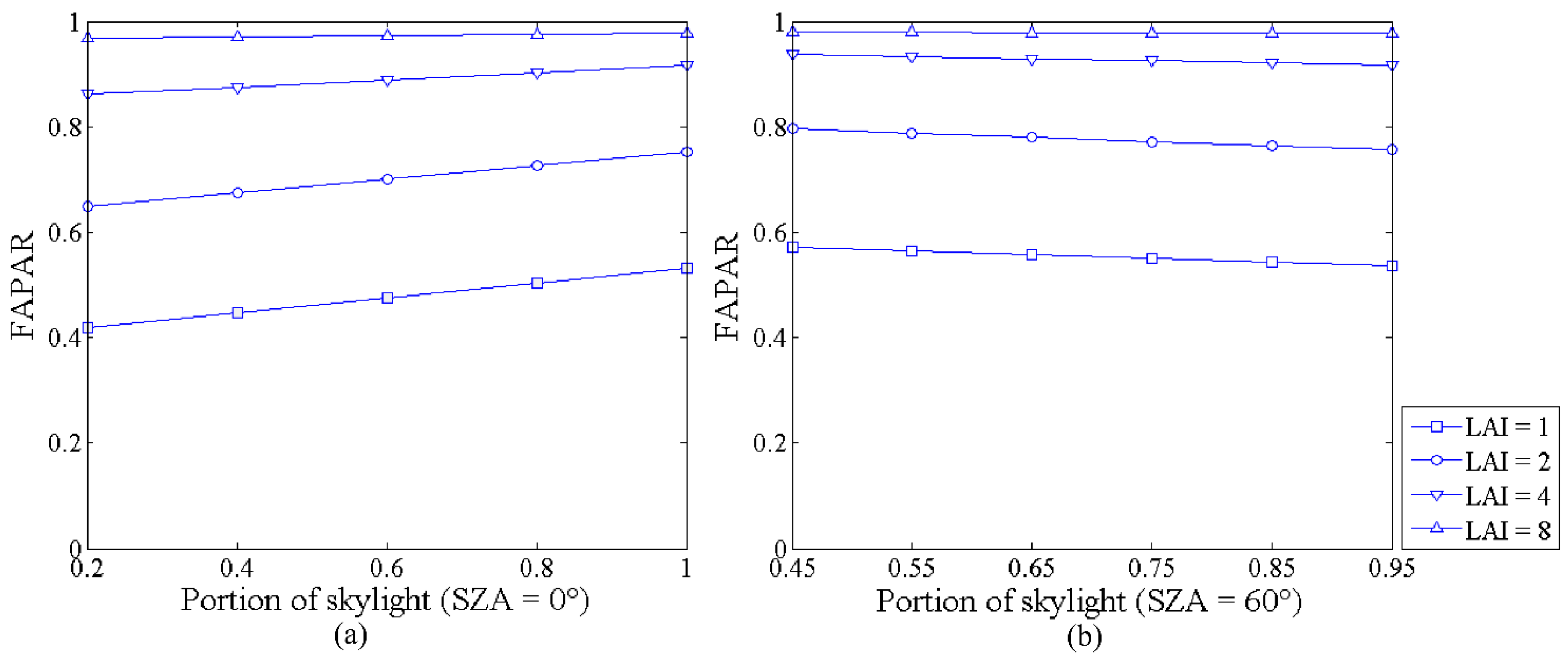
4.1.1. Sensitivities of FAPAR to Extra Skylight Proportions
4.1.2. Validating Temporal Normalization Method
4.1.3. Comparing Temporal Interpolation Methods
4.2. Estimating Fine-Resolution FAPAR and Spatial Scaling
4.3. Validating MODIS Product
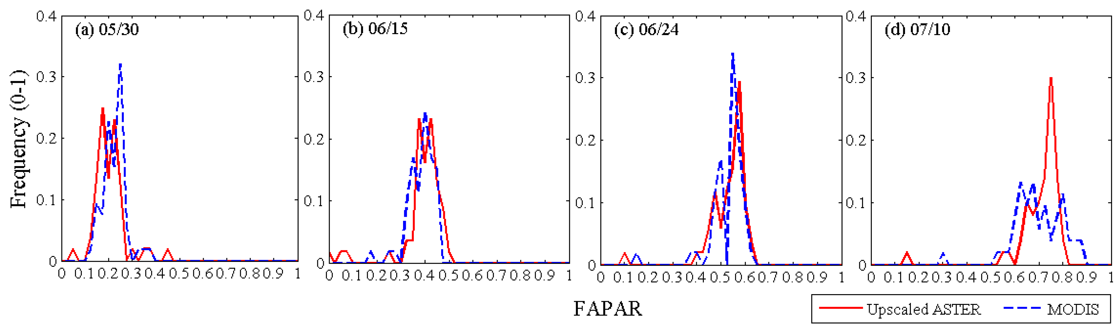
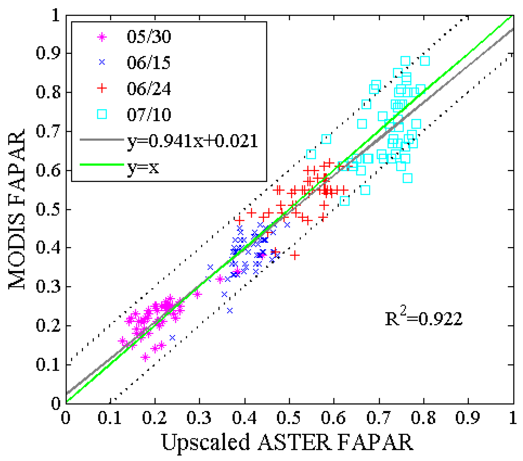
4.3.1. Spatial Comparison
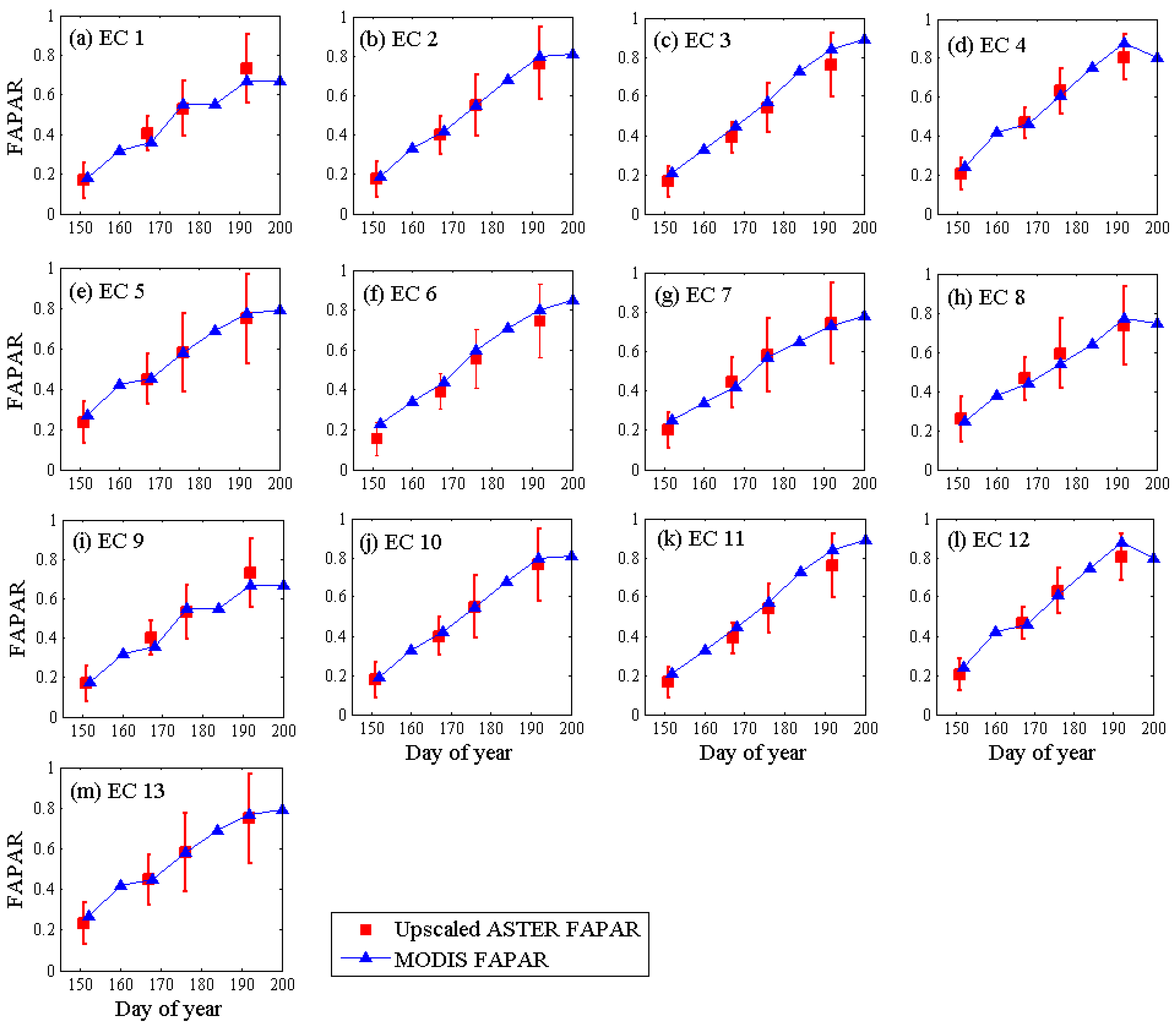
4.3.2. Temporal Validation
4.4. Discussion
5. Conclusions
Acknowledgments
Author Contributions
Conflicts of Interest
References
- Sellers, P.J.; Berry, J.A.; Collatz, G.J.; Field, C.B.; Hall, F.G. Canopy reflectance, photosynthesis, and transpiration, III. A reanalysis using improved leaf models and a new canopy integration scheme. Remote Sens. Environ. 1992, 42, 187–216. [Google Scholar] [CrossRef]
- Majasalmi, T.; Rautiainen, M.; Stenberg, P. Modeled and measured FPAR in a boreal forest: Validation and application of a new model. Agric. For. Meteorol. 2014, 189–190, 118–124. [Google Scholar] [CrossRef]
- Weiss, M.; Baret, F.; Garrigues, S.; Lacaze, R. LAI and FAPAR cyclopes global products derived from vegetation. Part 2: Validation and comparison with MODIS collection 4 products. Remote Sens. Environ. 2007, 110, 317–331. [Google Scholar] [CrossRef]
- Garrat, J.R. Sensitivity of climate simulations to land-surface and atmospheric boundary-layer treatments—A review. J. Clim. 1993, 6, 419–448. [Google Scholar] [CrossRef]
- McCallum, I.; Wagner, W.; Schmullius, C.; Shvidenko, A.; Obersteiner, M.; Fritz, S.; Nilsson, S. Comparison of four global FAPAR datasets over northern Eurasia for the year 2000. Remote Sens. Environ. 2010, 114, 941–949. [Google Scholar] [CrossRef]
- Fan, W.; Liu, Y.; Xu, X.; Chen, G.; Zhang, B. A new FAPAR analytical model based on the law of energy conservation: A case study in China. IEEE J. Sel. Top. Appl. Earth Obs. Remote Sens. 2014, 7, 3945–3955. [Google Scholar] [CrossRef]
- Cao, R.Y.; Shen, M.G.; Chen, J.; Tang, Y.H. A simple method to simulate diurnal courses of PAR absorbed by grassy canopy. Ecol. Indic. 2014, 46, 129–137. [Google Scholar] [CrossRef]
- Myneni, R.B.; Hoffman, S.; Knyazikhin, Y.; Privette, J.L.; Glassy, J.; Tian, Y.; Wang, Y.; Song, X.; Zhang, Y.; Smith, G.R.; et al. Global products of vegetation leaf area and fraction absorbed PAR from year one of MODIS data. Remote Sens. Environ. 2002, 83, 214–231. [Google Scholar] [CrossRef]
- Gobron, N.; Pinty, B.; Aussedat, O.; Chen, J.M.; Cohen, W.B.; Fensholt, R.; Gond, V.; Huemmrich, K.F.; Lavergne, T.; Méline, F.; et al. Evaluation of fraction of absorbed photosynthetically active radiation products for different canopy radiation transfer regimes: Methodology and results using joint research center products derived from Sea-WIFS against ground-based estimations. J. Geophys. Res. 2006, 111, 1–15. [Google Scholar] [CrossRef]
- Baret, F.; Hagolle, O.; Geiger, B.; Bicheron, P.; Miras, B.; Huc, M.; Berthelot, B.; Weiss, M.; Samain, O.; Roujean, J.L.; et al. LAI, FAPAR and FCOVER cyclopes global products derived from vegetation. Part 1: Principles of the algorithm. Remote Sens. Environ. 2007, 110, 275–286. [Google Scholar] [CrossRef]
- Gobron, N.; Pinty, B.; Aussedat, O.; Taberner, M. Uncertainty estimates for the FAPAR operational products derived from MERIS—Impact of top-of-atmosphere radiance uncertainties and validation with field data. Remote Sens. Environ. 2008, 112, 1871–1883. [Google Scholar] [CrossRef]
- GCOS. Systematic Observation Requirements for Satellite-Based Products for Climate; World Meteorological Organization: Geneva, Switzerland, 2011; p. 138. [Google Scholar]
- Fensholt, R.; Sandholt, I.; Rasmussen, M.S. Evaluation of MODIS LAI, FAPAR and the relation between FAPAR and NDVI in a semi-arid environment using in situ measurements. Remote Sens. Environ. 2004, 91, 490–507. [Google Scholar] [CrossRef]
- Tao, X.; Liang, S.L.; Wang, D.D. Assessment of five global satellite products of fraction of absorbed photosynthetically active radiation: Intercomparison and direct validation against ground-based data. Remote Sens. Environ. 2015, 163, 270–285. [Google Scholar] [CrossRef]
- Pickett-Heaps, C.A.; Canadell, J.G.; Briggs, P.R.; Gobron, N.; Haverd, V.; Paget, M.J.; Pinty, B.; Raupach, M.R. Evaluation of six satellite-derived fraction of absorbed photosynthetic active radiation (FAPAR) products across the australian continent. Remote Sens. Environ. 2014, 140, 241–256. [Google Scholar] [CrossRef]
- Martinez, B.; Camacho, F.; Verger, A.; Garcia-Haro, F.J.; Gilabert, M.A. Intercomparison and quality assessment of MERIS, MODIS and SEVIRI FAPAR products over the Iberian Peninsula. Int. J. Appl. Earth Obs. Geoinform. 2013, 21, 463–476. [Google Scholar] [CrossRef]
- D’Odorico, P.; Gonsamo, A.; Pinty, B.; Gobron, N.; Coops, N.; Mendez, E.; Schaepman, M.E. Intercomparison of fraction of absorbed photosynthetically active radiation products derived from satellite data over Europe. Remote Sens. Environ. 2014, 142, 141–154. [Google Scholar] [CrossRef]
- Meroni, M.; Atzberger, C.; Vancutsem, C.; Gobron, N.; Baret, F.; Lacaze, R.; Eerens, H.; Leo, O. Evaluation of agreement between space remote sensing SPOT-vegetation FAPAR time series. IEEE Trans. Geosci. Remote Sens. 2013, 51, 1951–1962. [Google Scholar] [CrossRef]
- FAO. Development of Standards for Essential Climate Variables: Fraction of Absorbed Photosynthetically Active Radiation (FAPAR). Available online: http://www.Fao.Org/gtos/doc/ecvs/t10/ecv-t10-fapar-report-v02.Doc (accessed on 2 August 2007).
- Goward, S.N.; Huemmrich, K.F. Vegetation canopy PAR absorptance and the normalized difference vegetation index—An assessment using the SAIL model. Remote Sens. Environ. 1992, 39, 119–140. [Google Scholar] [CrossRef]
- Yang, W.; Huang, D.; Tan, B.; Stroeve, J.; Shabanov, N.; Knyazikhin, Y.; Nemani, R.R.; Myneni, R.B. Analysis of leaf area index and fraction of PAR absorbed by vegetation products from the Terra MODIS sensor: 2000–2005. IEEE Trans. Geosci. Remote Sens. 2006, 44, 1829–1842. [Google Scholar] [CrossRef]
- Justice, C.; Tucker, C. Coarse resolution optical sensors. In The Sage Handbook of Remote Sensing; SAGE Publications Limited: London, UK, 2009; pp. 139–151. [Google Scholar]
- Iwata, H.; Ueyama, M.; Iwama, C.; Harazono, Y. Variations in fraction of absorbed photosynthetically active radiation and comparisons with MODIS data in burned black spruce forests of Interior Alaska. Pol. Sci. 2013, 7, 113–124. [Google Scholar] [CrossRef]
- Yang, F.; Ren, H.Y.; Li, X.Y.; Hu, M.G.; Yang, Y.P. Assessment of MODIS, MERIS, GEOV1 FPAR products over northern China with ground measured data and by analyzing residential effect in mixed pixel. Remote Sens. 2014, 6, 5428–5451. [Google Scholar] [CrossRef]
- Morisette, J.T.; Baret, F.; Privette, J.L.; Myneni, R.B.; Nickeson, J.E.; Garrigues, S.; Shabanov, N. V.; Weiss, M.; Fernandes, R.A.; Leblanc, S.G.; et al. Validation of global moderate-resolution LAI products: A framework proposed within the ceos land product validation subgroup. IEEE Trans. Geosci. Remote Sens. 2006, 44, 1804–1817. [Google Scholar] [CrossRef]
- Serbin, S.P.; Ahl, D.E.; Gower, S.T. Spatial and temporal validation of the MODIS LAI and FPAR products across a boreal forest wildfire chronosequence. Remote Sens. Environ. 2013, 133, 71–84. [Google Scholar] [CrossRef]
- Olofsson, P.; Eklundh, L. Estimation of absorbed PAR across Scandinavia from satellite measurements. Part II: Modeling and evaluating the fractional absorption. Remote Sens. Environ. 2007, 110, 240–251. [Google Scholar] [CrossRef]
- Huemmrich, K.F.; Privette, J.L.; Mukelabai, M.; Myneni, R.B.; Knyazikhin, Y. Time-series validation of MODIS land biophysical products in a Kalahari woodland, Africa. Int. J. Remote Sens. 2005, 26, 4381–4398. [Google Scholar] [CrossRef]
- Claverie, M.; Vermote, E.F.; Weiss, M.; Baret, F.; Hagolle, O.; Demarez, V. Validation of coarse spatial resolution LAI and FAPAR time series over cropland in southwest France. Remote Sens. Environ. 2013, 139, 216–230. [Google Scholar] [CrossRef]
- Wang, Y.; Xie, D.; Li, X. Universal scaling methodology in remote sensing science by constructing geographic trend surface. J. Remote Sens. 2014, 18, 1139–1146. [Google Scholar]
- Wang, Y.; Xie, D.; Li, Y. Downscaling remotely sensed land surface temperature over urban areas using trend surface of spectral index. J. Remote Sens. 2014, 18, 1169–1181. [Google Scholar]
- Li, X.; Cheng, G.; Liu, S.; Xiao, Q.; Ma, M.; Jin, R.; Che, T.; Liu, Q.; Wang, W.; Qi, Y.; et al. Heihe watershed allied telemetry experimental research (HiWATER): Scientific objectives and experimental design. Bull. Am. Meteorol. Soc. 2013, 94, 1145–1160. [Google Scholar] [CrossRef]
- Myneni, R.B.; Nemani, R.R.; Running, S.W. Estimation of global leaf area index and absorbed PAR using radiative transfer models. IEEE Trans. Geosci. Remote Sens. 1997, 35, 1380–1393. [Google Scholar] [CrossRef]
- Wang, J.F.; Christakos, G.; Hu, M.G. Modeling spatial means of surfaces with stratified nonhomogeneity. IEEE Trans. Geosci. Remote Sens. 2009, 47, 4167–4174. [Google Scholar] [CrossRef]
- Mu, X.; Huang, S.; Ren, H.; Yan, G.; Song, W.; Ruan, G. Validating GEOV1 fractional vegetation cover derived from coarse-resolution remote sensing images over croplands. IEEE J. Sel. Top. Appl. Earth Obs. Remote Sens. 2014, PP, 439–446. [Google Scholar] [CrossRef]
- Decagon Devices. Accupar PAR/LAI Ceptometer Model lp-80 Operator’s Manual (Version 1.0); Decagon Devices: Pullman, WA, USA, 2014. [Google Scholar]
- Xie, D.; Wang, Y.; Chen, Y.; Zhao, J. Hiwater: Dataset of Vegetation FPAR in the Middle Reaches of the Heihe River Basin; Heihe Plan Science Data Center: Lanzhou, China, 2013. [Google Scholar]
- Cheng, Y.-B.; Zhang, Q.; Lyapustin, A.I.; Wang, Y.; Middleton, E.M. Impacts of light use efficiency and FPAR parameterization on gross primary production modeling. Agric. For. Meteorol. 2014, 189–190, 187–197. [Google Scholar] [CrossRef]
- Vermote, E.F.; Tanr´e, D.; Deuze, J.L.; Herman, M.; Morcette, J.J. Second simulation of the satellite signal in the solar spectrum, 6S: An overview. IEEE Trans. Geosci. Remote Sens. 1997, 35, 675–686. [Google Scholar] [CrossRef]
- Zhang, M.; Ma, M.; Wang, X. Hiwater: Land Cover Map in the Core Experimental Area of Flux Observation Matrix; Heihe Plan Science Data Center: Lanzhou, China, 2014. [Google Scholar]
- Gobron, N.; Verstraete, M. Ecv t10: Fraction of Absorbed Photosynthetically Active Radiation (FAPAR). Essential Climate Variables; Global Terrestrial Observing System Rome: Rome, Italy, 2008; p. 23. [Google Scholar]
- Steinberg, D.C.; Goetz, S.J.; Hyer, E.J. Validation of MODIS F-PAR products in boreal forests of Alaska. IEEE Trans. Geosci. Remote Sens. 2006, 44, 1818–1828. [Google Scholar] [CrossRef]
- Weiss, M.; Baret, F.; Smith, G.J.; Jonckheere, I. Methods for in situ leaf area index measurement, part II: From gap fraction to leaf area index: Retrieval methods and sampling strategies. Agric. For. Meteorol. 2004, 121, 17–53. [Google Scholar]
- Smolander, S.; Stenberg, P. Simple parameterizations of the radiation budget of uniform broadleaved and coniferous canopies. Remote Sens. Environ. 2005, 94, 355–363. [Google Scholar] [CrossRef]
- Ruimy, A.; Kergoat, L.; Bondeau, A. Comparing global models of terrestrial net primary productivity (NPP): Analysis of differences in light absorption and light-use efficiency. Glob. Chang. Biol. 1999, 5, 56–64. [Google Scholar] [CrossRef]
- Zhang, X.; Friedl, M.A.; Schaaf, C.B.; Strahler, A.H.; Hodges, J.C.F.; Gao, F.; Reed, B.C.; Huete, A. Monitoring vegetation phenology using MODIS. Remote Sens. Environ. 2003, 84, 471–475. [Google Scholar] [CrossRef]
- Mu, X.; Liu, Y.; Yan, G.; Yao, Y. Fractional vegetation cover retrieval using multi-spatial resolution data and plant growth model. IGARSS 2010, 2010, 241–244. [Google Scholar]
- Knyazikhin, Y.; Glassy, J.; Privette, J.L.; Tian, Y.; Lotsch, A.; Zhang, Y.; Wang, Y.; Morisette, J.T.; Votava, P.; Myneni, R.B.; et al. MODIS Leaf Area Index (LAI) and Fraction of Photosynthetically Active Radiation Absorbed by Vegetation (FPAR) Product (MOD15) Algorithm Theoretical Basis Document. Available online: http://eospso.gsfc.nasa.gov/atbd/modistables.html (accessed on 10 September 2015).
- Myneni, R.B.; Hall, F.G.; Sellers, P.J.; Marshak, A.L. The interpretation of spectral vegetation indexes. IEEE Trans. Geosci. Remote Sens. 1995, 33, 481–486. [Google Scholar] [CrossRef]
- Prince, S.D.; Goward, S.N. Global primary production: A remote sensing approach. J. Biogeogr. 1995, 22, 815–835. [Google Scholar] [CrossRef]
- Begue, A. Leaf area index, intercepted photosynthetically active radiation, and spectral vegetation indices: A sensitivity analysis for regular-clumped canopies. Remote Sens. Environ. 1993, 46, 45–59. [Google Scholar] [CrossRef]
- Carlson, T.N.; Ripley, D.A. On the relation between NDVI, fractional vegetation cover, and leaf area index. Remote Sens. Environ. 1997, 62, 241–252. [Google Scholar] [CrossRef]
- Myneni, R.B.; Williams, D.L. On the relationship between FAPAR and NDVI. Remote Sens. Environ. 1994, 49, 200–211. [Google Scholar] [CrossRef]
- Holland, P.W.; Welsch, R.E. Robust regression using iteratively reweighted least-squares. Commun. Stat. Theory Methods 1977, A6, 813–827. [Google Scholar] [CrossRef]
- Robustfit. Available online: http://cn.mathworks.com/help/stats/robustfit.html (accessed on 12 December 2015).
- Kotchenova, S.Y.; Vermote, E.F.; Levy, R.; Lyapustin, A. Radiative transfer codes for atmospheric correction and aerosol retrieval: Intercomparison study. Appl. Opt. 2008, 47, 2215–2226. [Google Scholar] [CrossRef] [PubMed]
- Evaluation of Measurement Data—Guide to the Expression of Uncertainty in Measurement. Available online: http://www.iso.org/sites/JCGM/GUM/JCGM100/C045315e-html/C045315e.html?csnumber=50461 (accessed on 12 December 2015).
- Torres, G.; Vossenkemper, J.; Raun, W.; Taylor, R. Maize (Zea mays) leaf angle and emergence as affected by seed orientation at planting. Exp. Agric. 2011, 1, 1–14. [Google Scholar] [CrossRef]
- Fang, F. The Retrieval of Leaf Inclination Angle and Leaf Area Index in Maize. Master’s Thesis, University of Twente, Enschede, The Netherlands, 2015. [Google Scholar]
- Camacho, F.; Cemicharo, J.; Lacaze, R.; Baret, F.; Weiss, M. GEOV1: LAI, FAPAR essential climate variables and FCOVER global time series capitalizing over existing products. Part 2: Validation and intercomparison with reference products. Remote Sens. Environ. 2013, 137, 310–329. [Google Scholar] [CrossRef]
- Baret, F.; Weiss, M.; Lacaze, R.; Camacho, F.; Makhmara, H.; Pacholcyzk, P.; Smets, B. Geov1: LAI and FAPAR essential climate variables and Fcover global time series capitalizing over existing products. Part1: Principles of development and production. Remote Sens. Environ. 2013, 137, 299–309. [Google Scholar] [CrossRef]


| Categories | Temporal Info. | Spatial Info. | Description |
|---|---|---|---|
| In-situ measurement | 30 May 2012–18 July 2012 | 13 sites | Mobile measurement for 12 sites at approximate 5-day intervals and continuous stationary measurement for the left 1 site |
| MODIS FAPAR | 24 May 2012–10 July 2012 at 8-day intervals | scene h25v05 at 1 km resolution | MOD15A2 C5; ISIN projection |
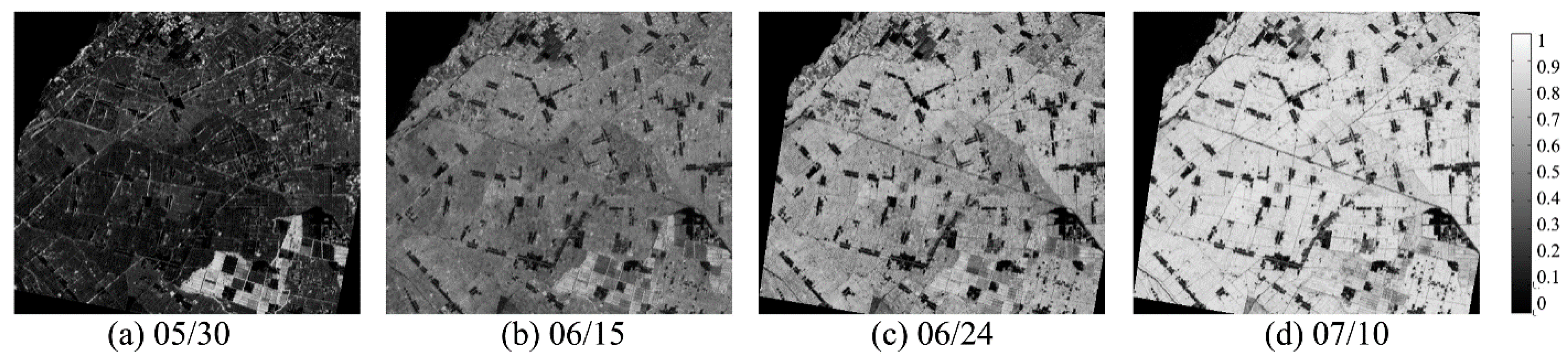
| ASTER images | 30 May 2012, 15 June 2012, 24 June 2012, 10 July 2012 | 15 m resolution | L1B product; UTM projection |
| SPOT-5 image | 10 August 2008 | 10 m resolution | Ancillary for geometric registration |
| Land cover classification | 25 June 2012 | 1 m resolution | Ancillary for geometric registration |
| Parameters | Symbol | Values or Data Sources |
|---|---|---|
| Leaf reflectance | LOPEX93 corresponding to maize | |
| Leaf transmittance | ||
| Soil reflectance | Field measurement | |
| Recollision probability | p | , where , and [44] |
| Projection of leaves per unit ground area on the plane perpendicular to the incident solar beam | G | 0.5 |
| Solar zenith angle (SZA) | 0~70 at 10° interval | |
| Effective leaf area index | LAI | 0~8 at interval of 1 |
| Portion of diffused skylight in total incident radiation | β | 0~1 |
| LAI | Fitted | RMSE of FAPAR from the Fitted k vs. | LAI | Fitted | RMSE of FAPAR from the Fitted k vs. | ||||
|---|---|---|---|---|---|---|---|---|---|
| k1 | k2 | Fitted FAPAR | Modelled FAPAR | k1 | k2 | Fitted FAPAR | Modelled FAPAR | ||
| 0.2 | 0.256 | 0.248 | 0.0007 | 0.0006 | 3 | 0.913 | 1.094 | 0.0010 | 0.0016 |
| 0.4 | 0.408 | 0.408 | 0.0084 | 0.0084 | 4 | 0.947 | 1.214 | 0.0010 | 0.0012 |
| 0.6 | 0.525 | 0.529 | 0.0050 | 0.0054 | 5 | 0.964 | 1.307 | 0.0010 | 0.0013 |
| 0.8 | 0.615 | 0.623 | 0.0009 | 0.0013 | 6 | 0.972 | 1.382 | 0.0000 | 0.0004 |
| 1 | 0.685 | 0.697 | 0.0080 | 0.0076 | 7 | 0.977 | 1.445 | 0.0000 | 0.0003 |
| 2 | 0.847 | 0.936 | 0.0009 | 0.0016 | 8 | 0.979 | 1.499 | 0.0010 | 0.0012 |
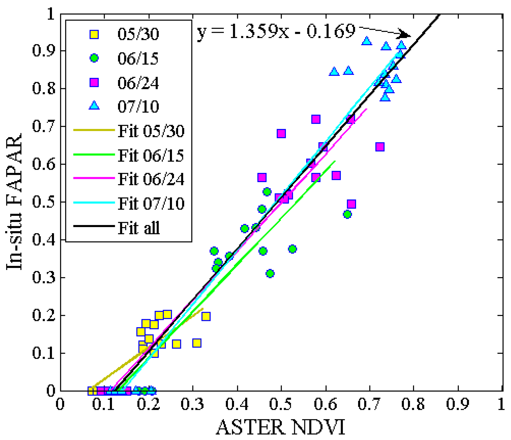
| Date | c1 * | c2 * | R2 | RMSE | p (c1) | p (c2) |
|---|---|---|---|---|---|---|
| 30 May | 0.839 | −0.055 | 0.619 | 0.052 | 0.000 | 0.148 |
| 15 June | 1.241 | −0.164 | 0.816 | 0.094 | 0.000 | 0.017 |
| 24 June | 1.290 | −0.148 | 0.896 | 0.095 | 0.000 | 0.013 |
| 10 July | 1.436 | −0.204 | 0.967 | 0.079 | 0.000 | 0.000 |
| All | 1.359 | −0.169 | 0.934 | 0.077 | 0.000 | 0.000 |
| Dates | Mean | Mean Absolute Difference | Standard Deviation of Difference |
|---|---|---|---|
| 30 May 2012 | 0.015 | 0.031 | 0.015 |
| 15 June 2012 | −0.025 | 0.039 | 0.011 |
| 24 June 2012 | −0.004 | 0.035 | 0.013 |
| 30 July 2012 | −0.022 | 0.072 | 0.034 |
© 2016 by the authors; licensee MDPI, Basel, Switzerland. This article is an open access article distributed under the terms and conditions of the Creative Commons by Attribution (CC-BY) license (http://creativecommons.org/licenses/by/4.0/).
Share and Cite
Wang, Y.; Xie, D.; Liu, S.; Hu, R.; Li, Y.; Yan, G. Scaling of FAPAR from the Field to the Satellite. Remote Sens. 2016, 8, 310. https://doi.org/10.3390/rs8040310
Wang Y, Xie D, Liu S, Hu R, Li Y, Yan G. Scaling of FAPAR from the Field to the Satellite. Remote Sensing. 2016; 8(4):310. https://doi.org/10.3390/rs8040310
Chicago/Turabian StyleWang, Yiting, Donghui Xie, Song Liu, Ronghai Hu, Yahui Li, and Guangjian Yan. 2016. "Scaling of FAPAR from the Field to the Satellite" Remote Sensing 8, no. 4: 310. https://doi.org/10.3390/rs8040310
APA StyleWang, Y., Xie, D., Liu, S., Hu, R., Li, Y., & Yan, G. (2016). Scaling of FAPAR from the Field to the Satellite. Remote Sensing, 8(4), 310. https://doi.org/10.3390/rs8040310