Article

Climatology Analysis of Aerosol Effect on Marine Water Cloud from Long-Term Satellite Climate Data Records

1
National Centers for Environmental Information (NCEI), NOAA/NESDIS, Asheville, NC 28801, USA
2
Center for Satellite Applications and Research (STAR), NOAA/NESDIS, Madison, WI 53706, USA
3
Cooperative Institute for Meteorological Satellite Studies (CIMSS), UW-Madison, Madison, WI 53706, USA
*
Author to whom correspondence should be addressed.
Remote Sens. 2016, 8(4), 300; https://doi.org/10.3390/rs8040300
Submission received: 27 January 2016 / Revised: 18 March 2016 / Accepted: 29 March 2016 / Published: 2 April 2016
(This article belongs to the Special Issue Satellite Climate Data Records and Applications)

Abstract

:
Satellite aerosol and cloud climate data records (CDRs) have been used successfully to study the aerosol indirect effect (AIE). Data from the Advanced Very High Resolution Radiometer (AVHRR) now span more than 30 years and allow these studies to be conducted from a climatology perspective. In this paper, AVHRR data are used to study the AIE on water clouds over the global oceans. Correlation analysis between aerosol optical thickness (AOT) and cloud parameters, including cloud droplet effective radius (CDER), cloud optical depth (COD), cloud water path (CWP), and cloud cover fraction (CCF), is performed. For the first time from satellite observations, the long-term trend in AIE over the global oceans is also examined. Three regimes have been identified: (1) AOT < 0.08, where CDER increases with AOT; (2) 0.08 < AOT < 0.3, where CDER generally decreases when AOT increases; and (3) AOT > 0.3, where CDER first increases with AOT and then levels off. AIE is easy to manifest in the CDER reduction in the second regime (named Regime 2), which is identified as the AIE sensitive/effective regime. The AIE manifested in the consistent changes of all four cloud variables (CDER, COD, CWP, and CCF) together is located only in limited areas and with evident seasonal variations. The long-term trend of CDER changes due to the AIE of AOT changes is detected and falls into three scenarios: Evident CDER decreasing (increasing) with significant AOT increasing (decreasing) and evident CDER decreasing with limited AOT increasing but AOT values fall in the AIE sensitive Regime 2.

Graphical Abstract

1. Introduction

Cloud microphysical structures and properties play an important role in the cloud-radiative-precipitation feedbacks and provide a critical link between the energy and hydrological cycles of Earth’s climate system. Atmospheric aerosol in the accumulation mode is the major source of cloud condensation nuclei and is therefore critical for the formation of cloud microphysical structures and properties [1,2,3]. Hygroscopic aerosol particles are called condensation nuclei (CN). A CN that can be activated by growth into the sub-micron size regime by absorption of water vapor in the cloud environment are called cloud condensation nuclei (CCN). Changes in atmospheric aerosols due to anthropogenic emissions will result in the modification of CCN and cloud microphysical properties, which will further change the cloud effect on the radiation budget and precipitation efficiency. This entire process is named as the aerosol indirect effect (AIE) [4,5,6,7,8,9,10].
Two types of aerosol indirect effect have been identified. The first type is called the first indirect effect (also named “Twomey effect” or “albedo effect”), which refers to the increase of cloud albedo due to cloud particle number increase and size reduction associated with the increase of aerosols under the assumption of constant cloud liquid water amount [4,5,6,9,11]. The second type is called the second indirect effect (also named “lifetime effect”), which refers to the prolonged cloud lifetime and cloud reflectance enhancement due to the reduction of precipitation efficiency resulted from cloud droplet number increase and size reduction induced from the increase of aerosols [7,10,12,13,14,15].
The first indirect effect has strong observational and modeling support. However, large ambiguities and uncertainties remain in the understanding of the second indirect effect. This is because the aerosol induced changes in cloud microphysical/optical properties (such as cloud liquid water amount, cloud optical depth, precipitation efficiency, etc.) are entangled with the changes in the cloud macrophysical properties (such as cloud height, cloud vertical motion, cloud lifetime, etc.) caused by cloud dynamics. These factors may suppress or amplify each other depending on the specific meteorological conditions and cloud regimes [10,16,17].
There have been many satellite observations, in-situ measurements and field campaigns of aerosol indirect effect in the past three decades trying to narrow the uncertainties of aerosol effect on cloud and precipitation. The in-situ and field measurements were mainly focused on process study of aerosol indirect effect for specific regions, seasons, and cloud types (e.g., [12,16,18,19,20,21,22,23,24]), while satellite observations were used either for studying the AIE for different aerosol loading scenarios in selected regions (e.g., [6,13,15,25,26,27,28,29,30]) or for determining the correlation relationships between the aerosol loading and cloud microphysical properties, such as cloud droplet size, liquid water amount, and cloud optical depth, in broader areas (such as over the ocean, land, or globe) by using limit length of satellite data records (e.g., [28,31,32,33,34,35,36,37]). Both field measurements and satellite observations of AIE have been used to develop databases for parameterization, initialization, and validation of regional and global climate models (e.g., [38,39,40,41,42,43,44,45,46]), which makes it possible to more accurately simulate the AIE processes and perform climatological analysis of the AIE on both regional and global scales (e.g., [46,47,48,49,50,51,52,53,54,55]). Due to the complexity of the AIE issues, remote sensing observation, in-situ measurement, and model simulation are often used together in the AIE investigation (e.g., [52,56,57]).
In this study, we analyze the correlation relationships between aerosol loading and cloud microphysical properties over global ocean for marine water clouds (mainly stratus and stratocumulus) from a climatology perspective by using more than 30-year climate data records (CDRs) of aerosols and clouds derived from the National Ocean and Atmospheric Administration (NOAA) operational satellite observations of the Advanced Very High Resolution Radiometer (AVHRR). Identifying the aerosol indirect effect signatures contained in the long-term AVHRR satellite observation and examining the changing trend of the AIE signatures are the two major objectives of this study. The results will benefit the determination of global AIE climatology, which, so far, is mainly based on long-term model simulations. The content of the paper is arranged as follows: AVHRR satellite aerosol and cloud climate data record (CDR) datasets used in our analyses are introduced in the next section, the AIE climatology analysis and results are provided in Section 3, summary and conclusions are given in the closing section.

2. Satellite Data

This study uses version 3 of NOAA operational satellite AVHRR aerosol optical thickness (AOT) CDR product and version 5.3 NOAA Pathfinder Atmospheres-Extended (PATMOS-x) AVHRR cloud CDR products. The AVHRR data comprise the longest operational global satellite observation of the Earth’s atmosphere and surface. Observed radiances/reflectances have been widely used to derive long-term products of atmospheric variables, such as cloud and aerosol. AVHRR radiances have been carefully re-calibrated recently using more accurate Moderate Resolution Imaging Spectroradiometer (MODIS) radiances to achieve a quality suitable for long-term trend studies [58,59,60]. For example, an examination of cloud amount and cloud optical depth time series demonstrated that the resultant AVHRR inter-satellite biases are less than 1% after cross-calibration with MODIS and retrospectively inter-calibrated among AVHRR sensors from NOAA-6, -7, -8, -9, -10, -11, -12, -14, -15, -16, -17, -18, and -19 satellites [61]. The newly calibrated AVHRR global area coverage (GAC) radiances in 1 km × 4 km spatial resolution are subsampled rather than averaged to 0.1° × 0.1° degree equal angle orbital grid in the PATMOS-x Level-2b CDR data [61].
PATMOS-x cloud products used in our analysis are cloud droplet effective radius (CDER), cloud optical depth (COD), cloud water path (CWP), and cloud cover fraction (CCF) for marine water clouds (mainly stratus and stratocumulus). Different algorithms [61,62] were used to derive these cloud products for daytime and nighttime, respectively, by using the inter-calibrated AVHRR GAC radiance data. They are output together with the inter-calibrated radiances and selected ancillary data (e.g., surface types) as the Level-2b daily CDR products, which allow other applications and CDRs to be generated from the PATMOS-x CDR data. PATMOS-x CDR data span from 1978 to present and should extend past 2020. Only the data after 1980 will be used in the current study in view of many missing observations in the first three years (1978–1980) of AVHRR data records. PATMOS-x cloud products also include five cloud types: warm liquid water, supercooled water-mixed phase, opaque ice, nonopaque high ice (cirrus), and cloud overlap (multiple cloud layers). The cloud types are determined using a multispectral algorithm developed for AVHRR using a series of cloud phase threshold tests from the infrared and near-infrared channels. Specifically, three sequential tests are involved in the determination of warm liquid water type: (1) brightness temperature of 11 µm channel larger than 273.16 K (the melting point of pure water); (2) cloud overlap test; and (3) cirrus test. A detailed description of the algorithm and its performance can be found in Pavolonis et al. [63]. Both warm liquid water cloud type and ocean surface type contained in the PATMOS-x CDR products are used to identify the marine water cloud in the current analysis.
AVHRR AOT CDR is derived over global water (or ocean) surface from the 0.63 µm channel using a two-channel AVHRR aerosol retrieval algorithm [64] from AVHRR clear-sky reflectance, which is determined from the PATMOS-x AVHRR all-sky reflectance and cloud probability products contained in version 5.3 PATMOS-x AVHRR reflectance/cloud CDRs. Due to the limited channels of AVHRR instrument, only aerosol retrievals over water can be obtained and only the AOT retrieved from 0.63 µm channel achieves climate quality. The retrievals from the spectrally wider 0.86 µm channel are contaminated by water vapor absorption, which is difficult to be accurately quantified, especially in the context of AOT trend. The AVHRR AOT retrieval algorithm had been carefully validated by comparing its results with those from the AERONET ground AOT measurement [64,65] and the MODIS satellite AOT observations [66]. It had been applied to the previous versions of PATMOS-x reflectance to generate long-term AOT data for the study of AOT long-term trend over global and regional scales [67,68,69]. Residual cloud contamination on AOT has been greatly reduced in version 3 AVHRR AOT CDR product compared to the previous versions. It is more reliable for trend studies due to improvement in the accurate cloud detection algorithm. The cloud detection used for the AOT CDR comes from version 5.3 PATMOS-x AVHRR cloud CDR products [70].
Global AVHRR AOT (at 0.63 µm channel) CDR daily products along with the corresponding Level-2b PATMOS-x AVHRR cloud CDR products are used in the current study. The data period spans from 1981 to 2011 and the spatial resolution is 0.1° × 0.1° degree on an equal angle orbital grid. AVHRR AOT retrieval can be problematic at larger solar zenith angles [71,72] beyond 60°N and 60°S latitudes (especially for the winter months), which may result in poor data sampling in monthly AOT averages in these regions. At the same time, cloud detection is degraded over bright snow and ice surfaces at polar latitudes. Thus, we will confine our analysis to within 60°S and 60°N over the global oceans. For a trend analysis, two-and-a-half years of data after the major volcano eruptions of El Chichón in March 1982 and Mt. Pinatubo in June 1991 were discarded to avoid the abrupt AOT perturbations [67].

3. Climatology Analysis and Results

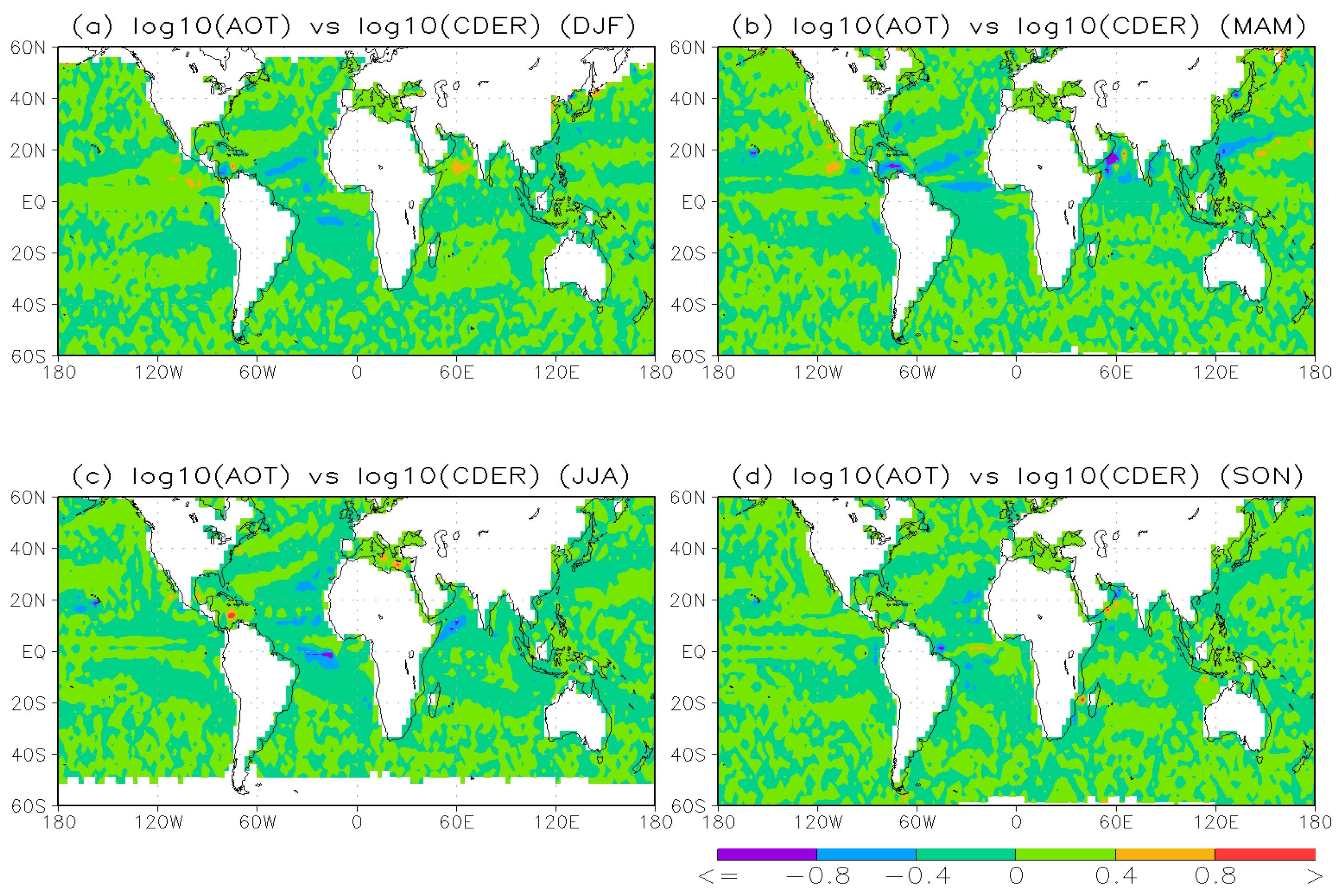
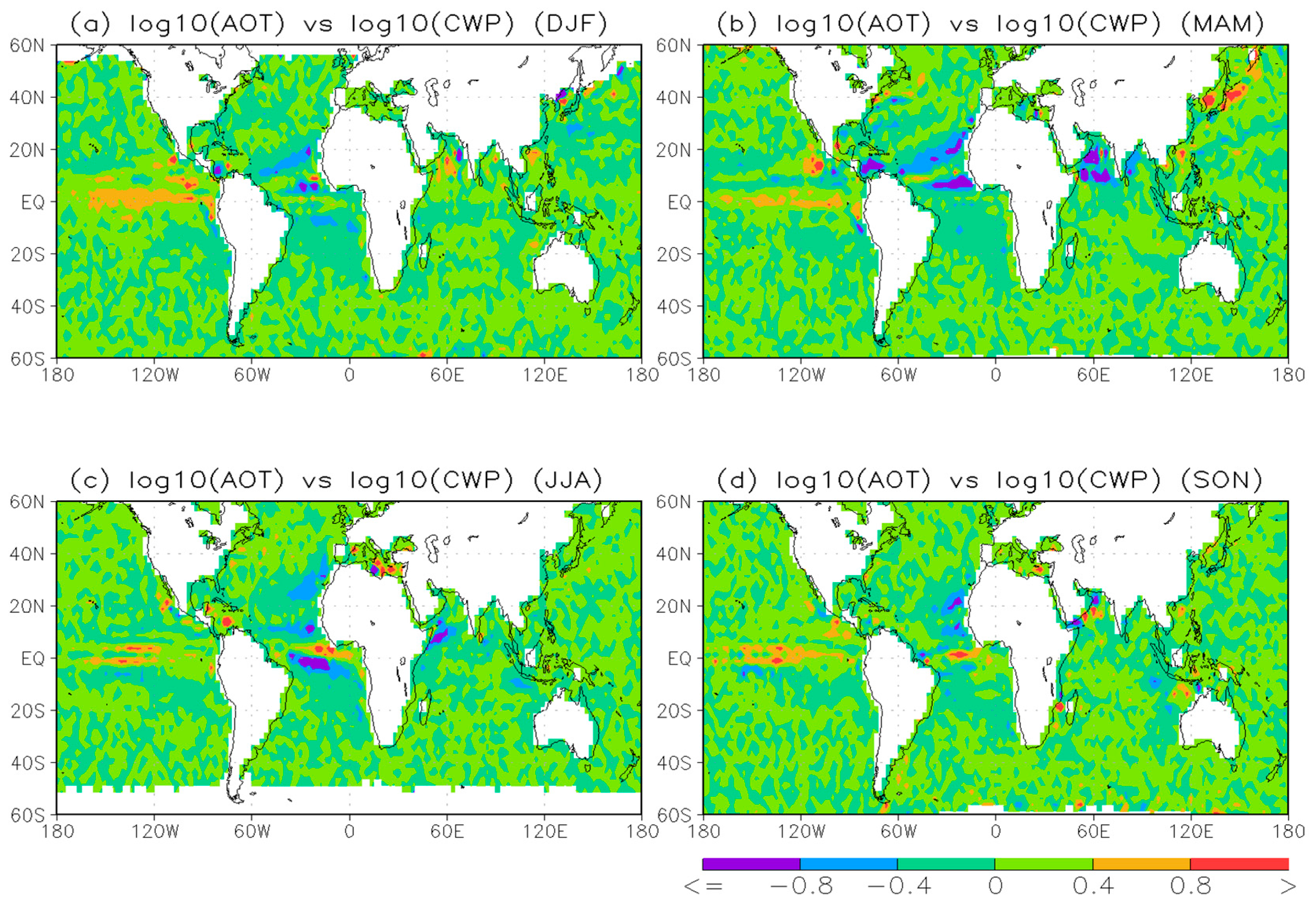
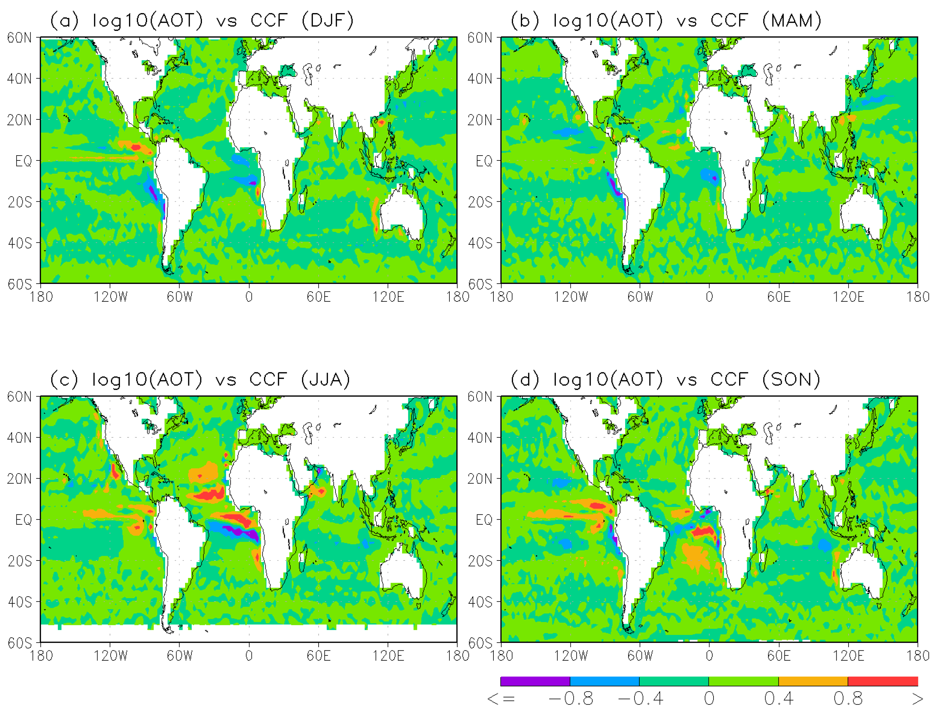
3.1. Analysis Methodology

In order to evaluate AIE of water clouds over global ocean using the satellite observation, we analyze the correlations between AOT (or τ), which is considered as a proxy of column aerosol concentration [9,28,33,36,37,73], and cloud parameters, including CDER (or re), COD (or τc), CWP, and CCF. CDER and COD are retrieved directly from the satellite radiances while CWP is computed from CDER and COD. Their relationship can be expressed by the following equation [74,75]:
r e = 9 5 × C W P ρ τ c
where ρ is the density of liquid water. When aerosol concentration increases (or AOT increases) and the cloud base is coupled with the marine boundary layer, more aerosols will be transported into the cloud layer to become activated CCN and grow to cloud droplets with smaller CDER given fixed cloud liquid water content (or constant CWP) [76,77]. Then COD will increase according to Equation (1). This chain of changes triggered by aerosol loading increase and described by Equation (1) with fixed CWP is the conventional first AIE mentioned in the introduction. Reduced CDER may further suppress precipitation efficiency and increase cloud lifetime and CCF along with the increase in CWP, which is the aforementioned conventional second AIE. Since CWP is derived from CDER and COD in our satellite observations, we hesitate to use CWP as an independent variable to detect the lifetime effect. However, CCF can be used as an independent variable to detect the cloud lifetime aerosol effect because it is derived independently from CDER and COD. A cloud detection algorithm based on the naïve Bayesian probabilistic methodology was used to determine PATMOS-x AVHRR cloud cover fraction. The algorithm was trained and validated by using CALIPSO (Cloud-Aerosol Lidar and Infrared Pathfinder Satellite Observations) lidar observations. For an AVHRR GAC pixel (~5 km in size), its cloud fraction was computed from five pixels of CALIPSO that were closest to the center of the AVHRR GAC pixel. Detailed description of the cloud detection algorithm can be found in Heidinger et al. [70].
Since the assumption of constant CWP in Equation (1) holds only occasionally for some scenarios in the real world due to the influence of cloud dynamics and meteorological circumstances, the conventional correlation changes of COD, CWP, and CCF with CDER (caused by increased aerosol loading) described in the first and second AIEs only hold for specific meteorological circumstances and cloud regimes [10]. Shao and Liu [73] found that the response of CDER, COD, CWP, and CCF to the increased aerosol loading for marine stratocumulus off the coast of California can be variable, which is determined by the coupled effects of aerosol loading and macro-scale cloud depth (or cloud dynamics) on cloud droplet size due to their coherent pattern. As a result, satellite derived correlation between AOT and CDER, COD, CWP, and CCF can be either negative, or positive, or neutral depending on the location and regime of the clouds [10,35,73]. Therefore, for the regions where AOT is negatively correlated with CDER from satellite observations, the AIE is manifested and detectable by the satellite observation. If positive correlations of AOT with COD, CWP, and CCF are also observed simultaneously in the same regions where AOT negatively correlated with CDER, the AIE detected by CDER reduction in the satellite observation is further manifested in the satellite observed changes in COD, CWP, and CCF. For the regions with positive or no correlation between AOT and CDER, the AIE may still happen but it is overridden by the cloud dynamic effect as suggested by Shao and Liu [73]. In this case, the AIE cannot be detected by the satellite observation.

3.2. Results

The analysis of the satellite AIE climatology, based on the long-term AVHRR cloud and aerosol climate data records, is presented in the following subsections.

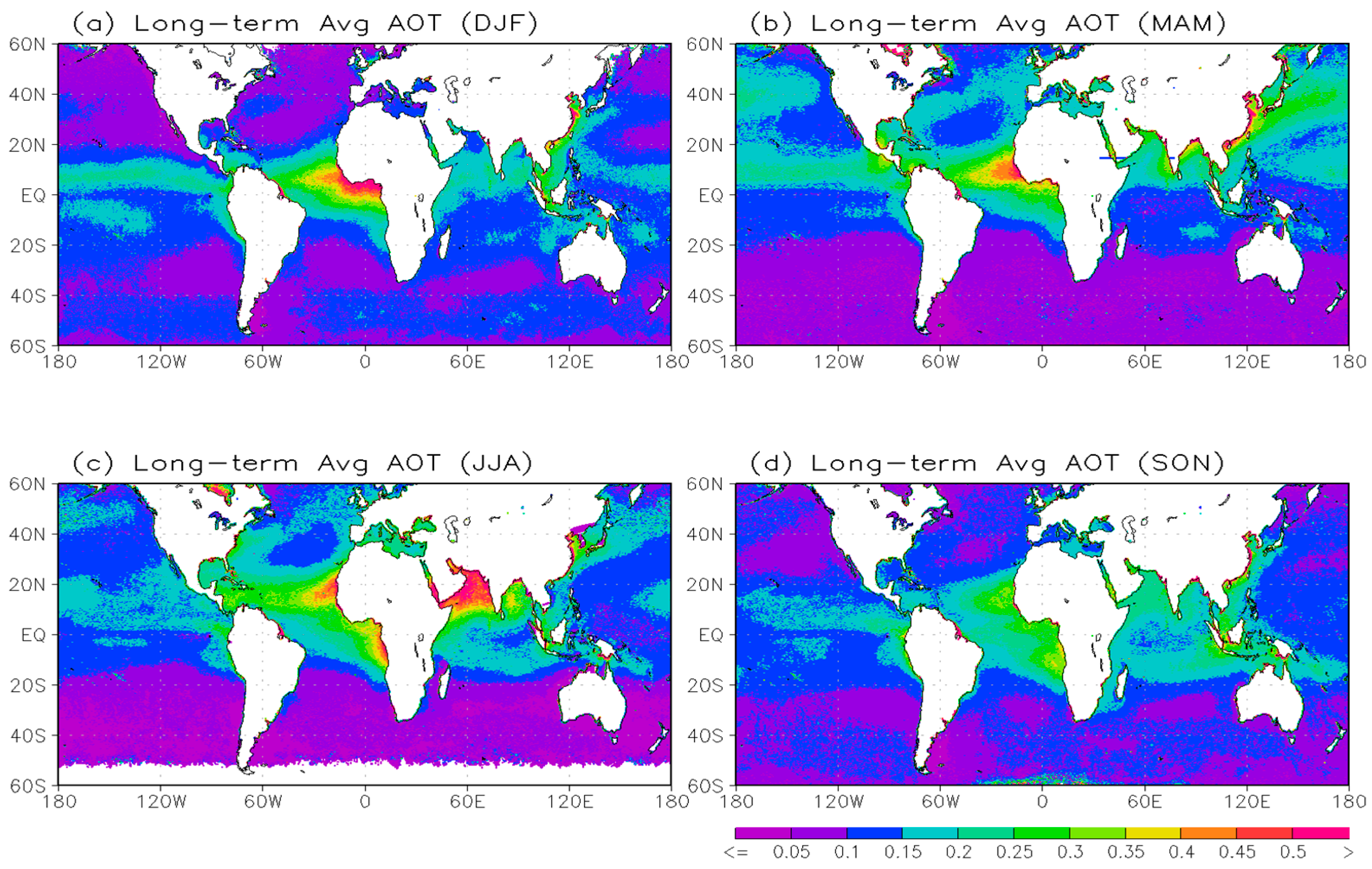
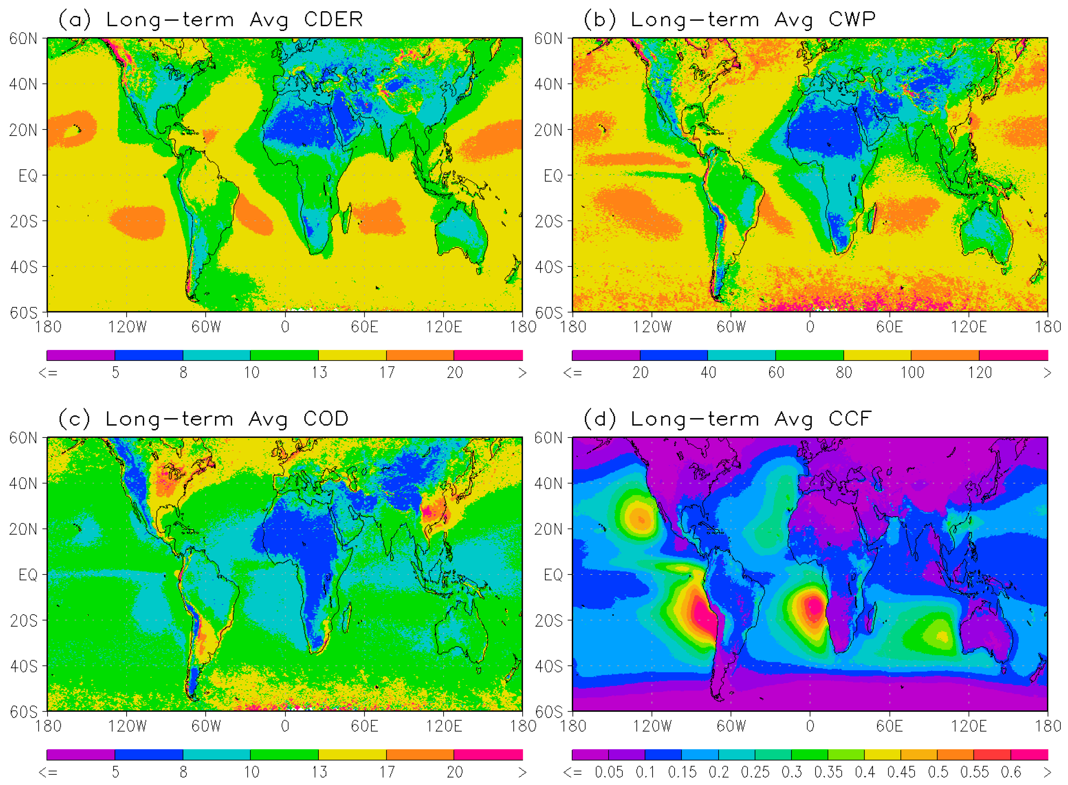
3.2.1. Long-Term Averages

Figure 1 shows the distribution of long-term (1981–2011) averaged monthly mean AOT over the global ocean. The 21 red boxes (see Table 1 also) mark the locations selected for regional survey studies shown later. It is seen the AOT values over the coastal oceanic regions are generally higher than those over the remote oceans due to the abundant continental aerosols flowing out from their source regions over land. For example these continental aerosols can include dust aerosols over the west coast of North Africa, biomass burning aerosols over the west coast of Central/South Africa, and industrial pollution and dust over Arabian Sea and the northeast coast of China. Most of these aerosols with continental origin are hygroscopic and can be transported into the cloud layer, especially in the coupled boundary condition [76], to become activated CCN and modify the cloud microphysical properties. AOT values over the northern hemisphere (NH) are generally higher than over the southern hemisphere (SH) due to the greater abundance of continental aerosols in the NH. Thus, it is not hard to imagine that the AIE should be more active in the NH than in the SH, which will be confirmed in the analysis below.
Global maps for long-term (1981–2011) averaged monthly mean CDER, CWP, COD, and CCF of water clouds are shown in Figure 2. It is seen in Figure 2a that CDER values are generally below 10 µm over land and larger than 10 µm and 13 µm over the coastal and remote oceans, respectively. This is because aerosol loadings over land source regions are generally higher than over oceanic regions so that the AIE is more active over land than over ocean. The AIE is also more active over the coastal oceans than over the remote oceans due to abundant continental aerosols outflow from land (see Figure 1). This land and ocean contrast of CDER due to the AIE was also noticed by some previous global studies based on relatively short-length of satellite observations [9,31,52]. It was found by Sekiguchi et al. [35] that reduced CDER can only be identified along coastal regions where abundant continental aerosols flow out from land rather than in remote oceanic regions. This is corroborated by the gradual CDER increase from the coastal oceanic regions (with the values in the range of 10–13 µm) to the remote oceanic regions (with the values larger than 13 µm) seen in Figure 2a. Mean AOT over NH oceans (~0.16) is also higher than its SH counterpart (~0.10) due to more continental aerosols in the NH. Correspondingly, CDER also shows consistent hemispheric contrast with a mean value of 12.5 µm in the NH and 14.2 µm in the SH. AIE emerges not only in the reduction of CDER but also in the increase of CWP and COD (see Figure 2b,c) over the east coastal regions of China and North America, Bolivia, Argentina, and North Atlantic Ocean (>40°N). It is hard to see any aerosol indirect effects in the distribution of CCF displayed in Figure 2d. However, it is worth mentioning some interesting features of CCF distribution, which may facilitate the CCF related AIE discussions later. Regions with higher CCF of water clouds are located in several oceanic areas near the west coasts of the continents (including California/Mexico, central South America, South Europe/North Africa, South Africa, and Australia) along with Arabian Sea and the southeast coast of China.
The zonal distribution of CDER for long-term averaged monthly mean data is displayed in Figure 3. It is seen CDER values over land are systemically lower than over ocean due to the AIE, which is consistent with the finding by Han et al. [31], Bréon et al. [9], and Suzuki et al. [52]. However, land and ocean contrast is not manifested in zonal mean COD, CWP, and CCF as in CDER (not shown).
Figure 4 shows the correlation plot between AOT and the logarithm of CDER for long-term averaged global monthly mean data. Three regimes can be identified: (1) AOT < 0.08, where CDER increases with AOT; (2) 0.08 < AOT < 0.3, where CDER generally decreases when AOT increases; and (3) AOT > 0.3, where CDER first increases with AOT and then levels off. A majority of the sample points falls in the second regime (named Regime 2 hereafter). When aerosol loading is low and falls in the first regime (named Regime 1 hereafter), the supersaturation is probably sufficient to maintain the activation of aerosols and their continuous growth to larger cloud droplets. Thus, CDER and AOT increase together. When aerosol loading reaches into Regime 2, more activated aerosols participate in the intense competition for the water vapor so that their growth to larger cloud droplets is suppressed. As a result, CDER decreases with AOT increases in Regime 2 (the first AIE), which becomes saturation in the negative response when AOT approaches to about 0.3. If aerosol loading further increases to the third regime (named Regime 3 hereafter), intense competition for water vapor evaporates the smaller droplets while the larger droplets will continue to grow at the expense of the smaller droplets until a new equilibrium is established. As a result, CDER increases first with AOT and levels off gradually in the Regime 3. Thus, the conventional AIE is only manifested in the form of CDER decreasing with AOT increasing in Regime 2.
A similar correlation feature in Regime 2 along with the AOT saturation threshold (~0.3) has been noticed in some previous global correlation studies based on limited-length of satellite observations (e.g., [27,33,35]). Even though the correlation features in Regimes 1 and 3 haven’t been reported in the previous observational studies, theoretic analysis and analytical model simulations (e.g., [3,27,78]) did find the correlation features similar to those identified in Regimes 1 and 3. Thus, it is worth to further exploring these two new regimes from both aspects of cloud microphysics and dynamics in future studies using model simulations, in-situ measurements and satellite observations.
The expected increase of COD associated with the decrease of CDER in Regime 2 due to the conventional AIE is not observed for the current long-term averaged monthly mean data. Sekiguchi et al. [35] pointed out that averaging procedures with shorter temporal periods (e.g., one day) in the satellite data analysis of aerosol–cloud interaction may produce different results from the averaging procedures with longer temporal periods (e.g., one month). The averaging process with longer temporal periods may obscure the cloud-aerosol interaction signature (such as the COD increase due to AIE). They suggested the daily averaging is more suitable for capturing the AIE signature than the monthly averaging for COD. By looking at the global maps of long-term averaged monthly mean CDER, COD, and CWP in Figure 2, we can see the AIE signature in the change of CDER is evident from land to coastal oceans and further to remote oceans while the AIE signature in the change of COD and CWP are only noticeable in limited locations. Thus, it is not hard to imagine the global statistics based on the long-term averaged monthly mean COD and CWP may damp or obscure the AIE signature contained in the COD (or CWP) change more than for CDER. At the same time, the averaging process may make some features associated with the cloud dynamic effect more distinct, which can also smear the AIE signature in the long-term averaged satellite observations.
To better identify the oceanic regions with clear manifestation of AIE in CDER, COD, CWP, and CCF, linear correlations between AOT and CDER, COD, CWP, and CCF have been calculated for 2.5° × 2.5° spatial grid over global oceans using their long-term averaged monthly mean values in 0.1° × 0.1° spatial resolution. Thus, the correlation coefficients reflect the relationship between AOT and each cloud variable in the spatial space.
Figure 5 shows global distribution of linear correlation slope for log10(AOT) vs. log10(CDER), log10(COD), log10(CWP), and CCF, respectively. The AIE manifested with distinct negative linear correlation slope of log10(AOT) vs. log10(CDER) is observed in Figure 5a over several oceanic areas: (a) a swath extending from the east coast of China to the North Pacific Ocean at about 20°N–40°N latitudes; (b) a swath extending from the east coast of USA to the North Atlantic Ocean at about 25°N–40°N latitudes; (c) Arabian Sea; (d) tropical and subtropical Atlantic Ocean (extending from the west coast of North and Central Africa to the east coast of Central America); (e) a belt area at about ~10°S of tropical South Pacific Ocean extending from the west coast of South America to about 130°W longitude; and (f) the west coast of central South America. These six areas extending from the coastal oceans with offshore continental aerosol influence to the remote oceans will be mentioned several times in the following discussions so that they are named hereafter as area “CH-NPO”, “US-NAO”, “AS”, “Tro-AO”, “Tro-SPO”, and “WcSAm”, respectively.
The AIE should manifest itself correspondingly as a positive linear correlation slope of log10(AOT) vs. log10(X) where X is any one of the cloud products used here (COD, CWP and CCF). The AIE signal in COD is seen only over three of the above six areas, CH-NPO, US-NAO, and WcSAm (see Figure 5b), with reduced spatial coverage. The AIE signal in CWP is only observed in CH-NPO and US-NAO areas but with much more reduced spatial coverage (see Figure 5c). The AIE signal in CCF is observed in CH-NPO and AS areas with much more reduced spatial coverage and magnitude (see Figure 5d). Distinct positive correlation between AOT and CCF is also observed in the west costal oceans of several continents (such as central South America, South Africa, and Australia), where higher cloud fraction of marine water clouds are expected (see Figure 2d) but the corresponding AIE signature is only somewhat noticeable in the AOT and CDER correlation (see Figure 5a) and is not observed in the correlation of AOT vs. COD and CWP (see Figure 5b,c). This is probably a signature of the second AIE (lifetime effect) but needs to be confirmed by future research. The distinct positive (or negative) correlation feature observed in the tropical uplifting zone of the atmospheric circulation (or the corresponding subsidence zones over the south and north subtropical oceans) may be a signature of the cloud dynamic effect rather than the signature of AIE, which also warrants a future investigation.

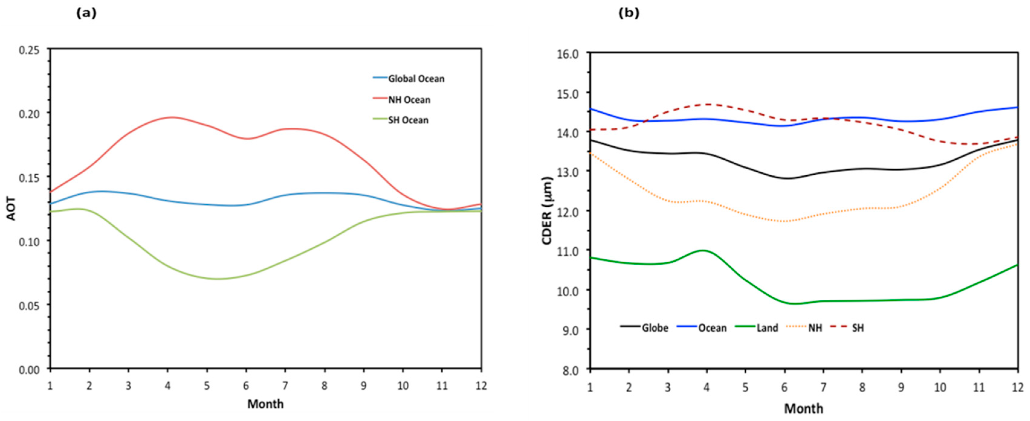
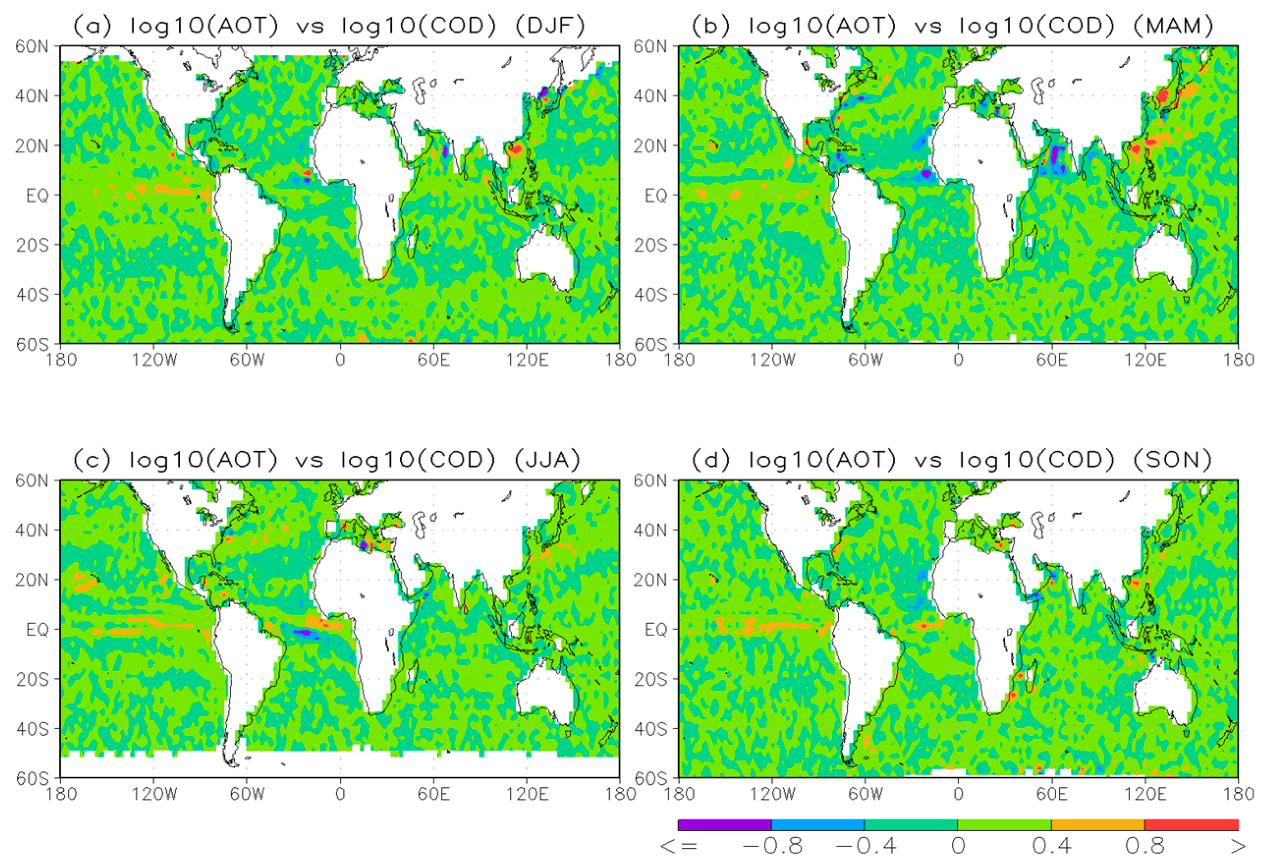
3.2.2. Seasonal Features

Long-term averaged AOT and CDER for each month are shown in Figure 6. AOT values averaged for NH oceans are evidently higher than that averaged for SH oceans in MAM (March, April, May), JJA (June, July, August), and early SON (September, October, November) but close to each other in late SON and early DJF (December, January, February). CDER over ocean is about 4 µm larger than over land for all months and the NH values are systemically lower than their SH counterparts for nearly all the months due to the AIE.
Global distribution maps of the long-term averaged AOT for each season are shown in Figure 7. There are distinct seasonal variations in AOT, especially in the oceanic regions influenced by continental aerosols due to dynamic transport. The outflow of continental aerosols to downstream coastal oceanic regions is the strongest in MAM and JJA, weakest in SON, and moderate in DJF.
The global maps of the linear correlation slope for log10(AOT) vs. log10(CDER), log10(COD), log10(CWP), and CCF in each season are shown in Figure 8, Figure 9, Figure 10 and Figure 11, respectively. For CDER (see Figure 8), the AIE manifested in CH-NPO, US-NAO, and AS areas (defined above in Figure 5) is most evident in MAM. The AIE in Tro-AO area is a year round feature with some changes in the exact location and intensity. The AIE in Tro-SPO and WcSAm areas is moderate and with less seasonal variations. The corresponding AIE manifested in COD appears only in CH-NPO area (maximal in both intensity and coverage in MAM) and US-NAO area (maximal in both intensity and coverage in JJA) in Figure 9. The AIE manifested in CWP enhancement, when considered together with the AIE of CDER and COD, is only noticeable for CH-NPO area in MAM and somewhat noticeable for US-NAO area in JJA (see Figure 10).
The AIE manifested in CCF enhancement in CH-NPO and AS areas (identified in Figure 5d) is more evident (see Figure 11) in MAM and JJA, respectively. MAM and JJA are the season that AOTs are also in the highest values, respectively, over the two areas (see Figure 7). The AIE manifested in CCF enhancement over the west coast of central South America is more evident in SON, which is consistent with the seasonal variations of AOT values in the region. The AIE manifested in CCF enhancement over the west coast of South Africa is more evident in JJA and SON, which are also the seasons that AOTs are in the highest values in the region. Thus, the AIE manifested clearly for all four cloud variables (CDER, COD, CWP, and CCF) together are in limited locations and with evident seasonal variations, but are generally consistent with the AOT seasonal variations.
It is noticed that the AIE signatures observed in the correlation analysis for all months in Figure 5 seem to be more evident and consistent than for individual seasons in Figure 8, Figure 9, Figure 10 and Figure 11. As we pointed out above, the averaging processes involved in deriving long-term averaged data may damp AIE signatures as well as boost the effect of cloud dynamics. We suspect the cloud dynamic effect is more prominent in the seasonal scale than in the monthly scale while the AIE signature is reversed. As a result, the AIE signature is less clear and consistent in the correlation based on the seasonal mean values than that based on the monthly mean values. More in-depth studies in the future are needed to confirm this hypothesis.

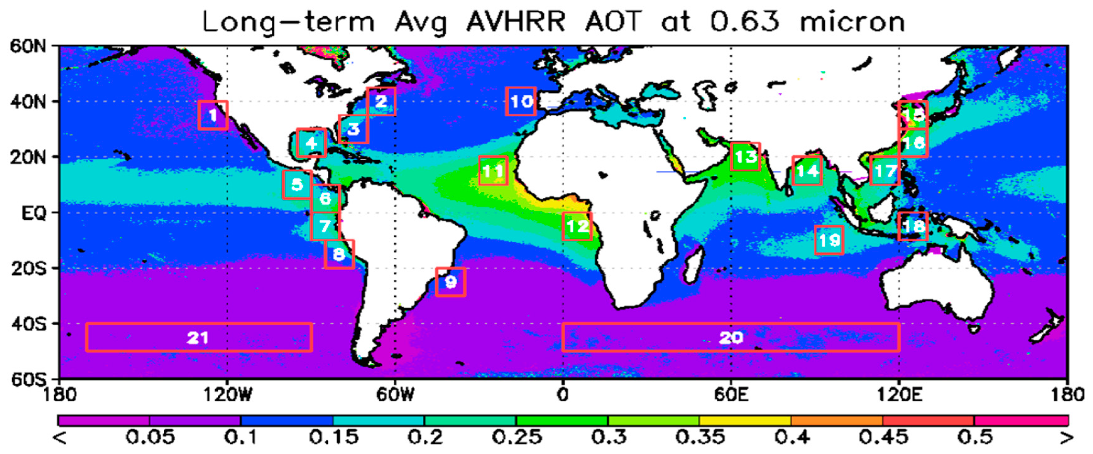
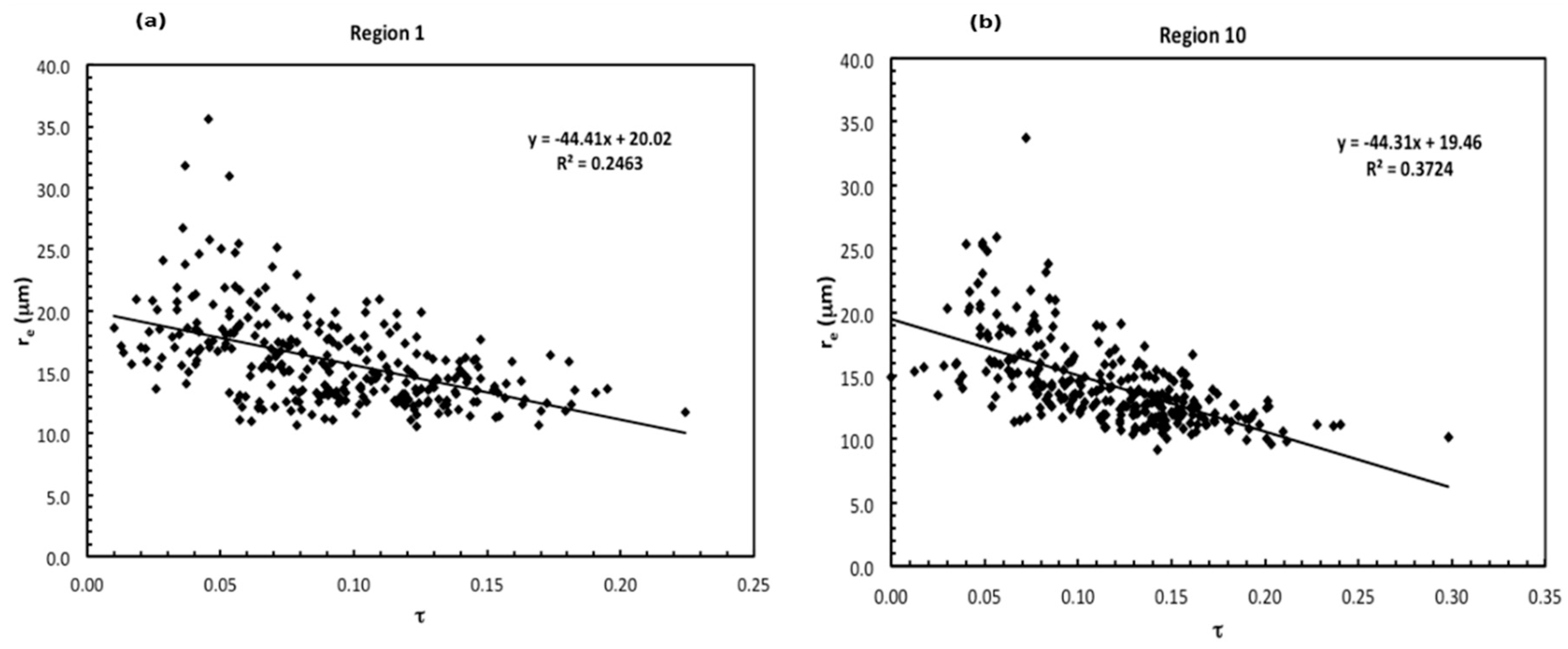
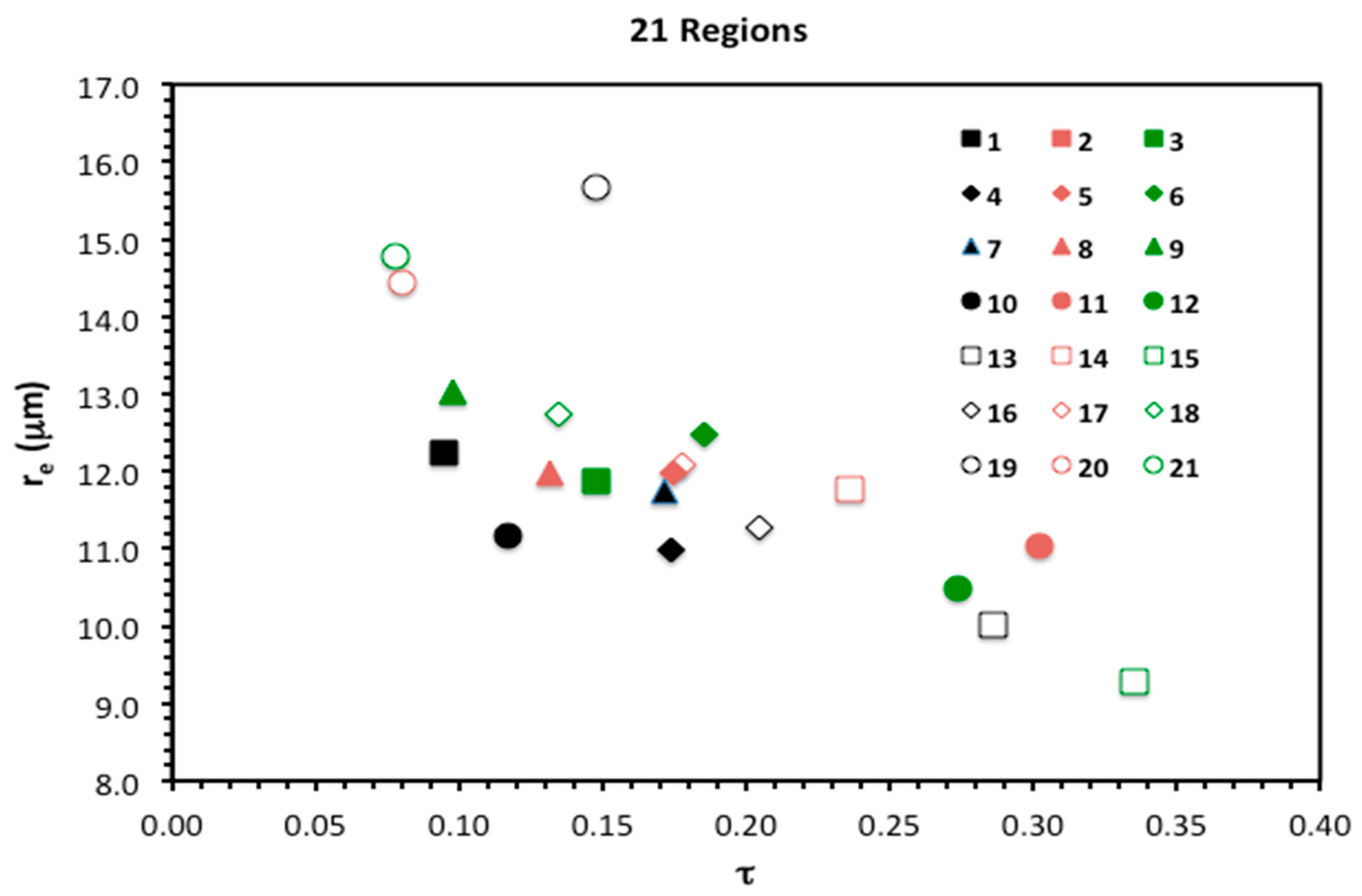
3.2.3. Regional Survey
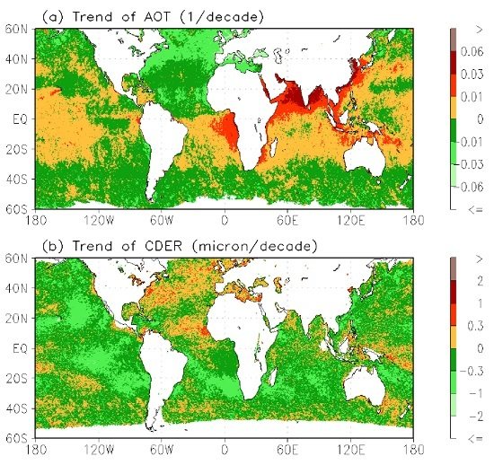
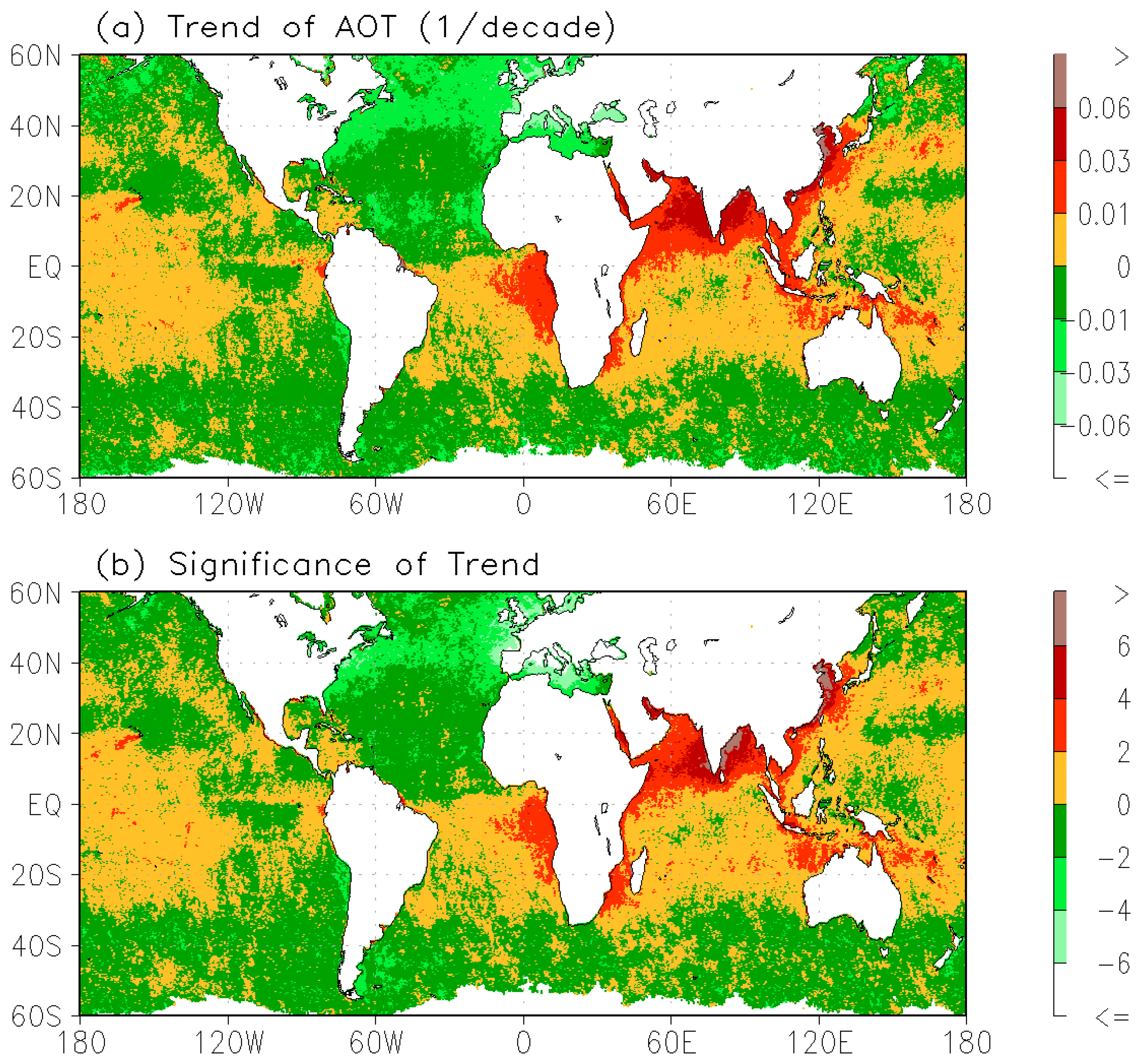
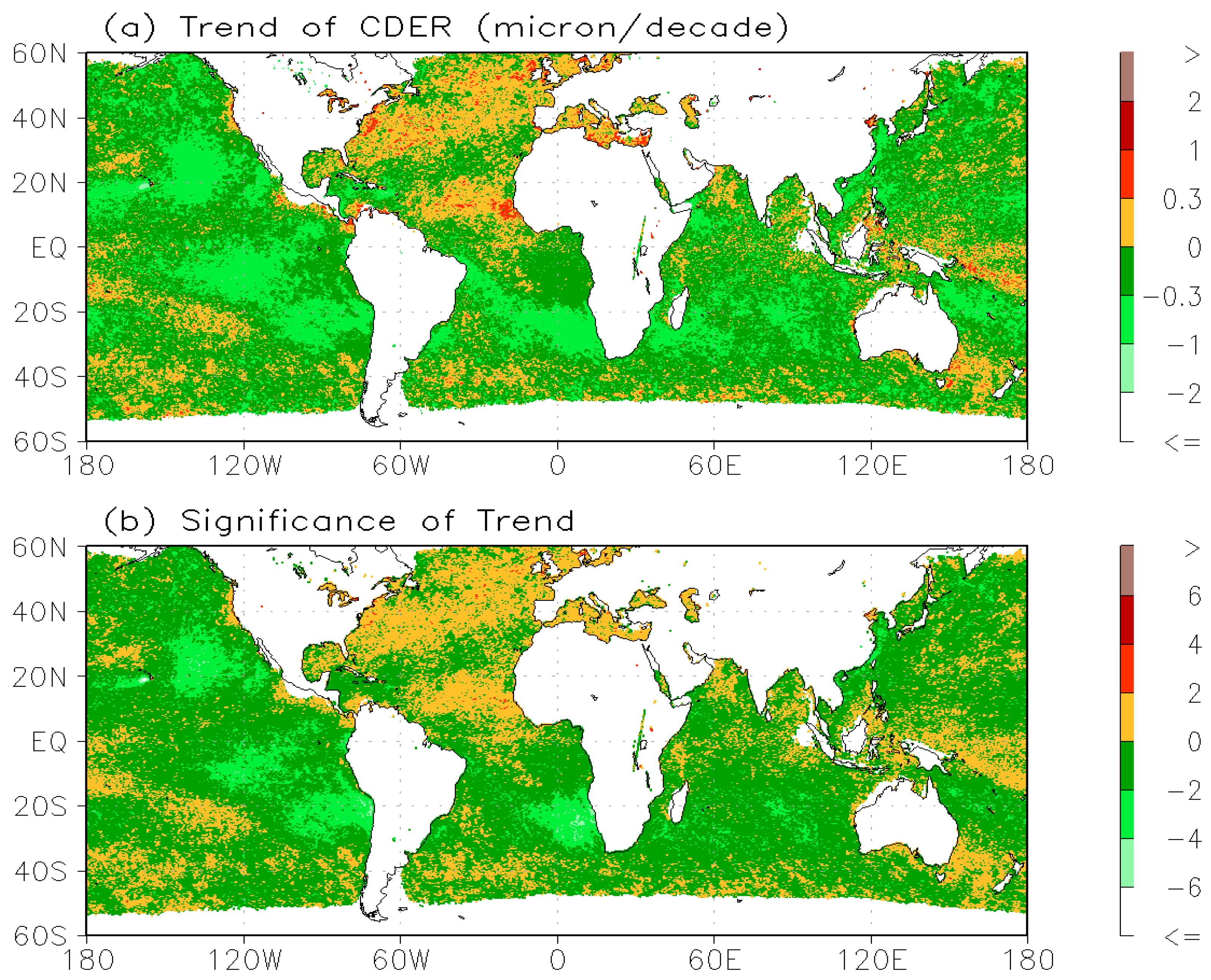
Twenty-one regions in both coastal and remote oceans marked by the red boxes in Figure 1 are selected for a regional survey study of AIE. These regions are listed in Table 1 for their geographic bounds. Regions 1–19 (coastal oceans), 20 (remote ocean), and 21 (remote ocean) cover an area of 10° (latitude) × 10° (longitude), 10° (latitude) × 120° (longitude), and 10° (latitude) × 80° (longitude), respectively. Figure 12 shows the regional averages of CDER vs. AOT for long-term averaged monthly mean values in the 21 regions. It is seen CDER systematically decreases with AOT increases from the remote marine regions (19, 20, 21) with relatively clean air to the offshore regions under the strong influence of continental aerosols, such as the dust in Region 11 (west coast of north Africa), the biomass burning in Region 12 (west coast of central Africa), and the industrial pollution and dust in Region 13 (Arabian Sea) and Region 15 (northeast coast of China). The AOT values in these regions also fall in the AIE sensitive Regime 2 identified above. Unlike long-term averaged monthly mean CDER, no monotonic changes of COD, CWP, and CCF with AOT are observed in these twenty-one regions.
Persistent marine stratus and stratus-cumulus cloud decks are frequently observed off the coasts of California (Region 1) and Southwest Europe (Region 10) and the intensive campaign studies of aerosol and cloud interaction have been performed in these two regions [16,23,28,79,80,81]. Figure 13 shows AOT vs. CDER for the monthly mean data averaged for Regions 1 and 10 over the time period from 1981 to 2011. The AOT values for the two regions indeed fall in AIE sensitive Regime 2 and there is clearly a decreasing trend of CDER along with AOT increase due to AIE. The negative correlation observed in Figure 13 is the AIE signature in the temporal space while the negative correlation observed in Figure 12 is the AIE signature in the spatial space.
In addition to the two coastal oceanic regions shown in Figure 13, we only find another four coastal oceanic regions among the 21 selected regions that show evident negative correlation between AOT and CDER. There is no evident positive correlation between AOT and COD (CWP, CCF) being found in the 21 regions. The linear correlation slope and correlation coefficient between AOT and CDER for the six coastal oceanic regions with evident negative correlation between AOT and CDER along with the typical aerosol types in the six regions are listed in Table 2.

3.2.4. Trend

The prominent advantage of using the long-term satellite CDR products for the correlation studies on the aerosol and cloud interaction is that we can examine the temporal trends of aerosol and cloud variables and investigate AIE in the context of long-term trend, which is not possible using satellite observations over shorter time periods. We will focus our trend study on the statistical linear tendency of CDER corresponding to AOT due to their evident correlation over global oceans identified in the above sections. The real tendencies of AOT and CDER may be much more complex than the statistical linear model. However, the linear trend allows for a simple approximation of the direction and magnitude of the changes in the data and may be adequate for many practical purposes. Results from the linear trend studies are not only commonly used by scientists but are also familiar to policy makers and the public. Thus, it is important to examine the climate change issues under such a linear model. We have successfully applied this linear trend analysis on the investigation of global and regional AOT changes and trends in some previous studies [67,68,69,82].
Here, we give a brief description on the linear trend analysis used in this study and a detailed description of linear trend analysis can be found in the literature (e.g., [83,84,85]). The linear change of a variable, such as CDER, is often measured with the linear trend (LT) in the unit of absolute (or percentage) changes per decade. CDER LT is the slope of linear regression line for the time series of monthly averaged CDER. We adopt the commonly used decision rule that a detectable trend is indicated at the 5% significance level or 95% confidence level, when |LT/σ| > 2 [85]. Here, σ is the standard deviation of CDER LT. It is difficult to determine σ from the observational data directly so that, as a first order approximation, we use the standard deviation (ε) of monthly averaged LT as σ after adjusting the unit of ε to match the unit of LT. We further name LT/σ ratio as the “significance” of CDER LT in this paper. A significance >+2 (or <−2) indicates the increasing (or decreasing) tendency detected is above 95% confidence level.
Figure 14 shows the global distribution of AOT linear trend (top panel) and the significance (bottom panel). It is seen that AOT increases evidently over the past three decades in the east coast of China, Arabian Sea, Bay of Bengal due to the industrial pollutions associated with fast economic growth in China and India. Evident AOT increases also observed over the west coast of central Africa and Southeast Asia due to the biomass burning. The AOT increase in these regions is above 95% confidence level. Distinct AOT reduction is observed over nearly the whole North Atlantic Ocean, especially over the east coast of USA and the coastal regions of Europe due to more rigid emission control in the developed countries. The AOT contributed from dust particles over the west coast of Sahara also tends to decrease in the past 30 years.
The corresponding global distribution of CDER linear trend (top panel) and the significance (bottom panel) is shown in Figure 15. Evident CDER decreasing trend is observed over the east coast of China due to enhanced AIE from AOT increase in the region. CDER increasing trend is observed over nearly the whole North Atlantic Ocean, especially over the east coast of USA, the coastal regions of Europe, and the west coast of Sahara. CDER increasing trend over these regions is due to the AIE compression since evident AOT decreasing is also observed over these regions. It is interesting to note that evident CDER decreasing trend is also observed over the broad oceanic regions extending from the west coasts of South/North America to the remote east oceanic regions of South/North Atlantic Ocean, which probably is also caused by the AIE enhancement since AOT increasing tendency (even though below 95% confidence level) is dominant in these regions (see Figure 14). Although AOT increasing trend is not significant in these regions but the AOT values (see Figure 1) are in the AIE sensitive Regime 2, which may still trigger active AIE and produce clear CDER decreasing trend. Likewise, evident CDER decreasing trend is also observed in the latitude belt between 20°S and 40°S of Indian and Atlantic Oceans, where AOT increasing trend is the dominant feature but below 95% confidence level. Since AOT values in these regions also fall in the AIE sensitive Regime 2, a minor AOT enhancement also produces intensive AIE and distinct CDER decreasing trend.

4. Summary and Conclusions

More than 30-year of satellite aerosol and cloud climate data records have been used to study the aerosol indirect effect of marine water clouds (mainly stratus and stratocumulus) over the global ocean from a climatology perspective. Correlation studies between aerosol optical thickness and cloud parameters (CDER, COD, CWP, and CCF) are performed and the long-term trend of AIE over the global ocean is examined for the first time using satellite observations. Three regimes of global AOT have been determined to identify potential AIE manifestation in CDER: (1) AOT < 0.08, where CDER increases with AOT; (2) 0.08 < AOT < 0.3, where CDER generally decreases when AOT increases; and (3) AOT > 0.3, where CDER first increases with AOT and then levels off. The AIE is manifested as CDER decreasing with AOT increasing only in Regime 2, which is the most common regime and defined as the AIE sensitive/effective regime. Although the AIE manifested in CDER is a global phenomenon, it is more evident over land and coastal oceans heavily influenced by continental aerosols arising from wind-blown dust, biomass burning, and industrial emissions. The AIE clearly manifested together in CDER and COD is evident in seasonal variations and located in limited areas: including a swath extending from the east coast of China to the North Pacific Ocean at about 20°N–40°N latitudes (CH-NPO area) and a swath extending from the east coast of USA to the North Atlantic Ocean at about 25°N–40°N latitudes (US-NAO area). The AIE clearly manifested together in all four cloud variables (CDER, COD, CWP, and CCF) is also observed in CH-NPO area. The intensity and spatial coverage are greatly reduced for COD, CWP, and CCF.
For the coastal oceanic areas, such as offshore California and southwest Europe, with persistent marine stratus and stratus-cumulus cloud decks and continent aerosol outflows where AOT is in Regime 2 (0.08 < AOT < 0.3), the AIE manifested in CDER is evident. This finding over ocean is similar to that found by Feingold et al. [27] over land. They noticed the response of CDER to aerosol loading in Brazilian biomass burning regions is the greatest in the region where AOT is relatively small.
A trend analysis based on the 30-year data record is presented. A decreasing (increasing) trend of CDER (AOT) is observed over the east coast of China. An increasing (decreasing) trend of CDER (AOT) is observed over nearly the whole North Atlantic Ocean, especially over the east coast of USA, the coastal regions of Europe, and the west coast of Sahara. A distinct CDER decreasing trend is also observed over the broad oceanic regions of South and North American west coasts and in the latitude belt between 20°S and 40°S of the Indian and Atlantic Oceans even though only a minor AOT increase is identified in these regions, although their AOT values are in the AIE sensitive Regime 2.
There are two caveats in our global statistical analysis based on long-term averaged monthly mean data. The first is the averaging process whose longer temporal period may damp or obscure the cloud-aerosol interaction signatures as well as make some features associated with the cloud dynamic effect more distinct. This enhanced cloud dynamic effect may also smear the AIE signatures in the long-term averaged observations. Thus, the major objective of the current study is to identify AIE signatures retained in the long-term averages and to detect the long-term trend of these AIE signatures. The aim is not to provide the physical mechanisms of AIE from the current global statistical analysis. Even though the analysis of instantaneous observations or short-term averaged data is more suitable for examining the physical mechanisms of AIE, the global statistical analysis and trend detection of AIE signatures are also important elements of the overall climate impact of aerosol–cloud interactions, which depend on long-term global observations. The second is related to the collocation of aerosol and cloud observations. Since aerosol retrievals are performed only for the clear-sky conditions, the collocation error of aerosol and cloud may impact the correlation analysis based on the long-term averaged data. This is especially true for any specific geographic location. Thus, we are very cautious on the interpretation of the strong regional correlation features between AOT and the cloud variables. Only those correlation features consistent for multiple cloud variables are interpreted as possible AIE signatures. Thus, it is important to identify AIE signatures for multiple cloud variables (such as CDER, COD, CWP, and CCF) and check the consistency of these signatures in both global and regional scales as well as in both spatial and temporal spaces.
It is generally agreed that AIE is a local to regional scale process acting on a short time scale. Therefore the instantaneous observations (or the data averaged in a short time period) over a regional scale should retain more AIE signatures than the global data averaged over a long time period. However, the fact that AIE signatures are retained in the global long-term averaged data does suggest that the regional and short time scale aerosol–cloud interaction process does contribute to the long-term global climate signal. Investigations of the physical mechanisms of aerosol–cloud interactions using the instantaneous or short-term observations at regional scales are clearly necessary. However, this paper makes the case that the study of the climate impact of aerosol–cloud interaction using long-term averaged global observations is also necessary. Studying AIE radiative forcing from a climatology perspective also becomes possible by using the AIE climatology identified in the current correlation and trend analysis, which will be our future work. The observational results from the current study will also benefit the modeling studies of aerosol–cloud interaction, especially in the context of the long-term climate effect.

Acknowledgments

This work is supported by the NOAA CDR program managed at the National Centers of Environment Information (NCEI) of NOAA/NESDIS. NCEI internal reviewers helped improve the paper. The constructive comments and suggestions provided by four anonymous reviewers were very helpful for improving the paper. The views, opinions, and findings contained in this paper are those of the author(s) and should not be construed as an official National Oceanic and Atmospheric Administration or U.S. Government position, policy, or decision.

Author Contributions

X. Zhao produced AVHRR aerosol CDR product, performed data analysis, and drafted the paper. A. Heidinger and A. Walther produced PATMOS-x AVHRR reflectance/cloud CDR products, provided help on the data analysis, improved and polished the paper.

Conflicts of Interest

The authors declare no conflict of interest.

Abbreviations

AERONET
Aerosol Robotic Network
AIE
Aerosol Indirect Effect
AOT(s)
Aerosol Optical Thickness(es)
AVHRR
Advanced Very High Resolution Radiometer
CALIPSO
Cloud-Aerosol Lidar and Infrared Pathfinder Satellite Observations
CCN
Cloud Condensation Nuclei
CDER
Cloud Droplet Effective Radius
CDR(s)
Climate Data Record(s)
CIMSS
Cooperative Institute for Meteorological Satellite Studies
CN
Condensation Nuclei
COD
Cloud Optical Depth
CWP
Cloud Water Path
GAC
Global Area Coverage
LT
Linear Trend
NCEI
National Centers for Environmental Information
NESDIS
National Environmental Satellite, Data, and Information Service
NH
Northern Hemisphere
NOAA
National Ocean and Atmospheric Administration
MODIS
Moderate Resolution Imaging Spectroradiometer
PATMOS-x
Pathfinder Atmospheres-Extended
SH
Southern Hemisphere
STAR
Center for Satellite Applications and Research

References

  1. Twomey, S. The nuclei of natural cloud formation, part II, the supersaturation in natural clouds and the variation of cloud droplet concentration. Pure Appl. Geophys. 1959, 43, 243–249. [Google Scholar] [CrossRef]
  2. Verheggen, B.; Cozic, J.; Weingartner, E.; Bower, K.; Mertes, S.; Connolly, P.; Gallagher, M.; Flynn, M.; Choularton, T.; Baltensperger, U. Aerosol partitioning between the interstitial and the condensed phase in mixed-phase clouds. J. Geophys. Res. Atmos. 2007, 112. [Google Scholar] [CrossRef]
  3. Mason, B.J. The Physics of Clouds; Clarendon Press: Oxford, UK, 2010. [Google Scholar]
  4. Twomey, S. Pollution and planetary albedo. Atmos. Environ. 1974, 8, 1251–1256. [Google Scholar] [CrossRef]
  5. Twomey, S.A.; Piepgrass, M.; Wolfe, T.L. An assessment of the impact of pollution on global cloud albedo. Tellus B 1984, 36, 356–366. [Google Scholar] [CrossRef]
  6. Coakley, J.A.; Bernstein, R.L.; Durkee, P.A. Effect of ship-stack effluents on cloud reflectivity. Science 1987, 237, 1020–1022. [Google Scholar] [CrossRef] [PubMed]
  7. Charlson, R.J.; Schwartz, S.E.; Hales, J.M.; Cess, R.D.; Coakley, J.A.; Hansen, J.E.; Hofmann, D.J. Climate forcing by anthropogenic aerosols. Science 1992, 255, 423–430. [Google Scholar] [CrossRef] [PubMed]
  8. Ramanathan, V.; Crutzen, P.J.; Kiehl, J.T.; Rosenfeld, D. Atmosphere—Aerosols, climate, and the hydrological cycle. Science 2001, 294, 2119–2124. [Google Scholar] [CrossRef] [PubMed]
  9. Breon, F.M.; Tanre, D.; Generoso, S. Aerosol effect on cloud droplet size monitored from satellite. Science 2002, 295, 834–838. [Google Scholar] [CrossRef] [PubMed]
  10. Stevens, B.; Feingold, G. Untangling aerosol effects on clouds and precipitation in a buffered system. Nature 2009, 461, 607–613. [Google Scholar] [CrossRef] [PubMed]
  11. Radke, L.F.; Coakley, J.A.; King, M.D. Direct and remote-sensing observations of the effects of ships on clouds. Science 1989, 246, 1146–1149. [Google Scholar] [CrossRef] [PubMed]
  12. Albrecht, B.A. Aerosols, cloud microphysics, and fractional cloudiness. Science 1989, 245, 1227–1230. [Google Scholar] [CrossRef] [PubMed]
  13. Kaufman, Y.J.; Fraser, R.S. The effect of smoke particles on clouds and climate forcing. Science 1997, 277, 1636–1639. [Google Scholar] [CrossRef]
  14. Kaufman, Y.J.; Koren, I. Smoke and pollution aerosol effect on cloud cover. Science 2006, 313, 655–658. [Google Scholar] [CrossRef] [PubMed]
  15. Rosenfeld, D.; Lohmann, U.; Raga, G.B.; O’Dowd, C.D.; Kulmala, M.; Fuzzi, S.; Reissell, A.; Andreae, M.O. Flood or drought: How do aerosols affect precipitation? Science 2008, 321, 1309–1313. [Google Scholar] [CrossRef] [PubMed]
  16. Lu, M.L.; Conant, W.C.; Jonsson, H.H.; Varutbangkul, V.; Flagan, R.C.; Seinfeld, J.H. The marine stratus/stratocumulus experiment (mase): Aerosol-cloud relationships in marine stratocumulus. J. Geophys. Res. Atmos. 2007, 112. [Google Scholar] [CrossRef]
  17. Stevens, B. Why are (precipitation mediated) aerosol effects on clouds so difficult to establish? Geochim. Cosmochim. Acta 2009, 73, A1274. [Google Scholar]
  18. Twohy, C.H.; Hudson, J.G. Measurements of cloud condensation nuclei spectra within maritime cumulus cloud droplets—Implications for mixing processes. J. Appl. Meteorol. 1995, 34, 815–833. [Google Scholar] [CrossRef]
  19. Leaitch, W.R.; Banic, C.M.; Isaac, G.A.; Couture, M.D.; Liu, P.S.K.; Gultepe, I.; Li, S.M.; Kleinman, L.; Daum, P.H.; MacPherson, J.I. Physical and chemical observations in marine stratus during the 1993 North Atlantic regional experiment: Factors controlling cloud droplet number concentrations. J. Geophys. Res. Atmos. 1996, 101, 29123–29135. [Google Scholar] [CrossRef]
  20. Brenguier, J.L.; Pawlowska, H.; Schuller, L.; Preusker, R.; Fischer, J.; Fouquart, Y. Radiative properties of boundary layer clouds: Droplet effective radius vs. number concentration. J. Atmos. Sci. 2000, 57, 803–821. [Google Scholar] [CrossRef]
  21. Pawlowska, H.; Brenguier, J.L. Microphysical properties of stratocumulus clouds during ACE-2. Tellus B 2000, 52, 868–887. [Google Scholar] [CrossRef]
  22. Brenguier, J.L.; Bakan, S. Eucrex-1994: An experimental study of the radiative properties of marine boundary-layer clouds—Preface. Atmos. Res. 2000, 55, 1–2. [Google Scholar] [CrossRef]
  23. Durkee, P.A.; Noone, K.J.; Bluth, R.T. The monterey area ship track experiment. J. Atmos. Sci. 2000, 57, 2523–2541. [Google Scholar] [CrossRef]
  24. Li, Z.Q.; Niu, F.; Fan, J.W.; Liu, Y.G.; Rosenfeld, D.; Ding, Y.N. Long-term impacts of aerosols on the vertical development of clouds and precipitation. Nat. Geosci. 2011, 4, 888–894. [Google Scholar] [CrossRef]
  25. Kaufman, Y.J.; Nakajima, T. Effect of amazon smoke on cloud microphysics and albedo—Analysis from satellite imagery. J. Appl. Meteorol. 1993, 32, 729–744. [Google Scholar] [CrossRef]
  26. Rosenfeld, D. Suppression of rain and snow by urban and industrial air pollution. Science 2000, 287, 1793–1796. [Google Scholar] [CrossRef] [PubMed]
  27. Feingold, G.; Remer, L.A.; Ramaprasad, J.; Kaufman, Y.J. Analysis of smoke impact on clouds in Brazilian biomass burning regions: An extension of Twomey’s approach. J. Geophys. Res. Atmos. 2001, 106, 22907–22922. [Google Scholar] [CrossRef]
  28. Matheson, M.A.; Coakley, J.A.; Tahnk, W.R. Aerosol and cloud property relationships for summertime stratiform clouds in the northeastern atlantic from advanced very high resolution radiometer observations. J. Geophys. Res. Atmos. 2005, 110. [Google Scholar] [CrossRef]
  29. Lin, J.C.; Matsui, T.; Pielke, R.A.; Kummerow, C. Effects of biomass-burning-derived aerosols on precipitation and clouds in the Amazon Basin: A satellite-based empirical study. J. Geophys. Res. Atmos. 2006, 111. [Google Scholar] [CrossRef]
  30. Koren, I.; Martins, J.V.; Remer, L.A.; Afargan, H. Smoke invigoration vs. inhibition of clouds over the amazon. Science 2008, 321, 946–949. [Google Scholar] [CrossRef] [PubMed]
  31. Han, Q.Y.; Rossow, W.B.; Lacis, A.A. Near-global survey of effective droplet radii in liquid water clouds using ISCCP data. J. Clim. 1994, 7, 465–497. [Google Scholar] [CrossRef]
  32. Han, Q.Y.; Rossow, W.B.; Zeng, J.; Welch, R. Three different behaviors of liquid water path of water clouds in aerosol-cloud interactions. J. Atmos. Sci. 2002, 59, 726–735. [Google Scholar] [CrossRef]
  33. Wetzel, M.A.; Stowe, L.L. Satellite-observed patterns in stratus microphysics, aerosol optical thickness, and shortwave radiative forcing. J. Geophys. Res. Atmos. 1999, 104, 31287–31299. [Google Scholar] [CrossRef]
  34. Nakajima, T.; Higurashi, A.; Kawamoto, K.; Penner, J.E. A possible correlation between satellite-derived cloud and aerosol microphysical parameters. Geophys. Res. Lett. 2001, 28, 1171–1174. [Google Scholar] [CrossRef]
  35. Sekiguchi, M.; Nakajima, T.; Suzuki, K.; Kawamoto, K.; Higurashi, A.; Rosenfeld, D.; Sano, I.; Mukai, S. A study of the direct and indirect effects of aerosols using global satellite data sets of aerosol and cloud parameters. J. Geophys. Res. Atmos. 2003, 108. [Google Scholar] [CrossRef]
  36. Kaufman, Y.J.; Koren, I.; Remer, L.A.; Rosenfeld, D.; Rudich, Y. The effect of smoke, dust, and pollution aerosol on shallow cloud development over the Atlantic Ocean. Proc. Natl. Acad. Sci. USA 2005, 102, 11207–11212. [Google Scholar] [CrossRef] [PubMed]
  37. Loeb, N.G.; Schuster, G.L. An observational study of the relationship between cloud, aerosol and meteorology in broken low-level cloud conditions. J. Geophys. Res. Atmos. 2008, 113. [Google Scholar] [CrossRef]
  38. Ghan, S.J.; Chuang, C.C.; Penner, J.E. A parameterization of cloud droplet nucleation part I: Single aerosol type. Atmos. Res. 1993, 30, 198–221. [Google Scholar] [CrossRef]
  39. Menon, S.; Del Genio, A.D.; Koch, D.; Tselioudis, G. GCM simulations of the aerosol indirect effect: Sensitivity to cloud parameterization and aerosol burden. J. Atmos. Sci. 2002, 59, 692–713. [Google Scholar] [CrossRef]
  40. Menon, S.; Brenguier, J.L.; Boucher, O.; Davison, P.; Del Genio, A.D.; Feichter, J.; Ghan, S.; Guibert, S.; Liu, X.H.; Lohmann, U.; et al. Evaluating aerosol/cloud/radiation process parameterizations with single-column models and second aerosol characterization experiment (ACE-2) cloudy column observations. J. Geophys. Res. Atmos. 2003, 108. [Google Scholar] [CrossRef]
  41. Brenguier, J.L.; Pawlowska, H.; Schuller, L. Cloud microphysical and radiative properties for parameterization and satellite monitoring of the indirect effect of aerosol on climate. J. Geophys. Res. Atmos. 2003, 108. [Google Scholar] [CrossRef]
  42. Pawlowska, H.; Brenguier, J.L. An observational study of drizzle formation in stratocumulus clouds for general circulation model (GCM) parameterizations. J. Geophys. Res. Atmos. 2003, 108. [Google Scholar] [CrossRef]
  43. Morrison, H.; Curry, J.A.; Khvorostyanov, V.I. A new double-moment microphysics parameterization for application in cloud and climate models. Part I: Description. J. Atmos. Sci. 2005, 62, 1665–1677. [Google Scholar] [CrossRef]
  44. Morrison, H.; Curry, J.A.; Shupe, M.D.; Zuidema, P. A new double-moment microphysics parameterization for application in cloud and climate models. Part II: Single-column modeling of arctic clouds. J. Atmos. Sci. 2005, 62, 1678–1693. [Google Scholar] [CrossRef]
  45. Rotstayn, L.D.; Liu, Y.G. Sensitivity of the first indirect aerosol effect to an increase of cloud droplet spectral dispersion with droplet number concentration. J. Clim. 2003, 16, 3476–3481. [Google Scholar] [CrossRef]
  46. Rotstayn, L.D.; Liu, Y.G. Cloud droplet spectral dispersion and the indirect aerosol effect: Comparison of two treatments in a GCM. Geophys. Res. Lett. 2009, 36. [Google Scholar] [CrossRef]
  47. Rotstayn, L.D. Indirect forcing by anthropogenic aerosols: A global climate model calculation of the effective-radius and cloud-lifetime effects. J. Geophys. Res. Atmos. 1999, 104, 9369–9380. [Google Scholar] [CrossRef]
  48. Rotstayn, L.D.; Liu, Y.G. A smaller global estimate of the second indirect aerosol effect. Geophys. Res. Lett. 2005, 32. [Google Scholar] [CrossRef]
  49. Lohmann, U.; Feichter, J.; Penner, J.; Leaitch, R. Indirect effect of sulfate and carbonaceous aerosols: A mechanistic treatment. J. Geophys. Res. Atmos. 2000, 105, 12193–12206. [Google Scholar] [CrossRef]
  50. Lohmann, U.; Koren, I.; Kaufman, Y.J. Disentangling the role of microphysical and dynamical effects in determining cloud properties over the Atlantic. Geophys. Res. Lett. 2006, 33. [Google Scholar] [CrossRef]
  51. Lohmann, U.; Feichter, J. Global indirect aerosol effects: A review. Atmos. Chem. Phys. 2005, 5, 715–737. [Google Scholar] [CrossRef]
  52. Suzuki, K.; Nakajima, T.; Numaguti, A.; Takemura, T.; Kawamoto, K.; Higurashi, A. A study of the aerosol effect on a cloud field with simultaneous use of GCM modeling and satellite observation. J. Atmos. Sci. 2004, 61, 179–194. [Google Scholar] [CrossRef]
  53. Cheng, Y.J.; Lohmann, U.; Zhang, J.H. Contribution of changes in sea surface temperature and aerosol loading to the decreasing precipitation trend in southern China. J. Clim. 2005, 18, 1381–1390. [Google Scholar] [CrossRef]
  54. Chou, C.; Neelin, J.D.; Lohmann, U.; Feichter, J. Local and remote impacts of aerosol climate forcing on tropical precipitation. J. Clim. 2005, 18, 4621–4636. [Google Scholar] [CrossRef]
  55. Morrison, H.; Pinto, J.O. Mesoscale modeling of springtime arctic mixed-phase stratiform clouds using a new two-moment bulk microphysics scheme. J. Atmos. Sci. 2005, 62, 3683–3704. [Google Scholar] [CrossRef]
  56. Qian, Y.; Gong, D.Y.; Fan, J.W.; Leung, L.R.; Bennartz, R.; Chen, D.L.; Wang, W.G. Heavy pollution suppresses light rain in China: Observations and modeling. J. Geophys. Res. Atmos. 2009, 114. [Google Scholar] [CrossRef]
  57. Bennartz, R.; Fan, J.W.; Rausch, J.; Leung, L.R.; Heidinger, A.K. Pollution from china increases cloud droplet number, suppresses rain over the east China sea. Geophys. Res. Lett. 2011, 38. [Google Scholar] [CrossRef]
  58. Heidinger, A.K.; Cao, C.Y.; Sullivan, J.T. Using moderate resolution imaging spectrometer (MODIS) to calibrate advanced very high resolution radiometer reflectance channels. J. Geophys. Res. Atmos. 2002, 107. [Google Scholar] [CrossRef]
  59. Cao, C.; Weinreb, M.; Xu, H. Predicting simultaneous nadir overpasses among polar-orbiting meteorological satellites for the intersatellite calibration of radiometers. J. Atmos. Ocean. Technol. 2004, 21, 537–542. [Google Scholar] [CrossRef]
  60. Heidinger, A.K.; Straka, W.C.; Molling, C.C.; Sullivan, J.T.; Wu, X.Q. Deriving an inter-sensor consistent calibration for the AVHRR solar reflectance data record. Int. J. Remote Sens. 2010, 31, 6493–6517. [Google Scholar] [CrossRef]
  61. Heidinger, A.K.; Foster, M.J.; Walther, A.; Zhao, X.P. The pathfinder atmospheres-extended AVHRR climate dataset. Bull. Am. Meteorol. Soc. 2014, 95. [Google Scholar] [CrossRef]
  62. Walther, A.; Heidinger, A.K. Implementation of the daytime cloud optical and microphysical properties algorithm (DCOMP) in PATMOS-x. J. Appl. Meteorol. Clim. 2012, 51, 1371–1390. [Google Scholar] [CrossRef]
  63. Pavolonis, M.J.; Heidinger, A.K.; Uttal, T. Daytime global cloud typing from AVHRR and VIIRS: Algorithm description, validation, and comparisons. J. Appl. Meteorol. 2005, 44, 804–826. [Google Scholar] [CrossRef]
  64. Zhao, X.-P.; Dubovik, O.; Smirnov, A.; Holben, B.N.; Sapper, J.; Pietras, C.; Voss, K.J.; Frouin, R. Regional evaluation of an advanced very high resolution radiometer (AVHRR) two-channel aerosol retrieval algorithm. J. Geophys. Res. 2004, 109, D02204. [Google Scholar] [CrossRef]
  65. Zhao, X.-P.; Laszlo, I.; Holben, B.N.; Pietras, C.; Voss, K.J. Validation of two-channel VIRS retrievals of aerosol optical thickness over ocean and quantitative evaluation of the impact from potential subpixel cloud contamination and surface wind effect. J. Geophys. Res. Atmos. 2003, 108. [Google Scholar] [CrossRef]
  66. Zhao, X.-P.; Laszlo, I.; Minnis, P.; Remer, L. Comparison and analysis of two aerosol retrievals over the ocean in the terra/clouds and the earth’s radiant energy system—Moderate resolution imaging spectroradiometer single scanner footprint data: 1. Global evaluation. J. Geophys. Res. Atmos. 2005, 110. [Google Scholar] [CrossRef]
  67. Zhao, X.-P.; Laszlo, I.; Guo, W.; Heidinger, A.; Cao, C.; Jelenak, A.; Tarpley, D.; Sullivan, J. Study of long-term trend in aerosol optical thickness observed from operational AVHRR satellite instrument. J. Geophys. Res. 2008, 113, D07201. [Google Scholar] [CrossRef]
  68. Zhao, X.-P.; Heidinger, A.K.; Knapp, K.R. Long-term trends of zonally averaged aerosol optical thickness observed from operational satellite AVHRR instrument. Meteorol. Appl. 2011, 18, 440–445. [Google Scholar] [CrossRef]
  69. Zhao, X.P. Satellite observed aerosol optical thickness and trend around megacities in the coastal zone. Adv. Meteorol. 2015, 2015, 170672-7. [Google Scholar] [CrossRef]
  70. Heidinger, A.K.; Evan, A.T.; Foster, M.J. A naive Bayesian cloud-detection scheme derived from Calipso and applied withing PATMOS-x. J. Appl. Meteorol. Clim. 2012. [Google Scholar] [CrossRef]
  71. Stowe, L.L.; Ignatov, A.M.; Singh, R.R. Development, validation, and potential enhancements to the second-generation operational aerosol product at the national environmental satellite, data, and information service of the national oceanic and atmospheric administration. J. Geophys. Res. Atmos. 1997, 102, 16923–16934. [Google Scholar] [CrossRef]
  72. Ignatov, A.; Stowe, L. Aerosol retrievals from individual AVHRR channels. Part I: Retrieval algorithm and transition from dave to 6 s radiative transfer model. J. Atmos. Sci. 2002, 59, 313–334. [Google Scholar] [CrossRef]
  73. Shao, H.F.; Liu, G.S. Why is the satellite observed aerosol’s indirect effect so variable? Geophys. Res. Lett. 2005, 32. [Google Scholar] [CrossRef]
  74. Stephens, G.L. Radiation profiles in extended water clouds. 1. Theory. J. Atmos. Sci. 1978, 35, 2111–2122. [Google Scholar] [CrossRef]
  75. Bennartz, R. Global assessment of marine boundary layer cloud droplet number concentration from satellite. J. Geophys. Res. Atmos. 2007, 112, D02201. [Google Scholar]
  76. Dong, X.Q.; Schwantes, A.C.; Xi, B.K.; Wu, P. Investigation of the marine boundary layer cloud and CCN properties under coupled and decoupled conditions over the azores. J. Geophys. Res. Atmos. 2015, 120, 6179–6191. [Google Scholar] [CrossRef]
  77. Logan, T.; Xi, B.K.; Dong, X.Q. Aerosol properties and their influences on marine boundary layer cloud condensation nuclei at the arm mobile facility over the Azores. J. Geophys. Res. Atmos. 2014, 119, 4859–4872. [Google Scholar] [CrossRef]
  78. Pruppacher, H.R.; Klett, J.D. Microphysics of Clouds and Precipitation; Kluwer Academy: Dordrecht, the Netherlands, 1997. [Google Scholar]
  79. Johnson, D.W.; Osborne, S.; Wood, R.; Suhre, K.; Johnson, R.; Businger, S.; Quinn, P.K.; Wiedensohler, A.; Durkee, P.A.; Russell, L.M.; et al. An overview of the Lagrangian experiments undertaken during the North Atlantic regional aerosol characterisation experiment (ACE-2). Tellus B 2000, 52, 290–320. [Google Scholar] [CrossRef]
  80. Brenguier, J.L.; Chuang, P.Y.; Fouquart, Y.; Johnson, D.W.; Parol, F.; Pawlowska, H.; Pelon, J.; Schuller, L.; Schroder, F.; Snider, J. An overview of the ACE-2 cloudycolumn closure experiment. Tellus B 2000, 52, 815–827. [Google Scholar] [CrossRef] [Green Version]
  81. Raes, F.; Bates, T.; McGovern, F.; Van Liedekerke, M. The 2nd aerosol characterization experiment (ACE-2): General overview and main results. Tellus B 2000, 52, 111–125. [Google Scholar] [CrossRef]
  82. Zhao, T.X.P.; Chan, P.K.; Heidinger, A.K. A global survey of the effect of cloud contamination on the aerosol optical thickness and its long-term trend derived from operational AVHRR satellite observations. J. Geophys. Res. Atmos. 2013, 118, 2849–2857. [Google Scholar] [CrossRef]
  83. Tiao, G.C.; Reinsel, G.C.; Xu, D.M.; Pedrick, J.H.; Zhu, X.D.; Miller, A.J.; Deluisi, J.J.; Mateer, C.L.; Wuebbles, D.J. Effects of autocorrelation and temporal sampling schemes on estimates of trend and spatial correlation. J. Geophys. Res. Atmos. 1990, 95, 20507–20517. [Google Scholar] [CrossRef]
  84. Wilks, D.S. Statistical Methods in the Atmosphere Sciences; Academic Press: San Diego, CA, USA, 1995. [Google Scholar]
  85. Weatherhead, E.C.; Reinsel, G.C.; Tiao, G.C.; Meng, X.L.; Choi, D.S.; Cheang, W.K.; Keller, T.; DeLuisi, J.; Wuebbles, D.J.; Kerr, J.B.; et al. Factors affecting the detection of trends: Statistical considerations and applications to environmental data. J. Geophys. Res. Atmos. 1998, 103, 17149–17161. [Google Scholar] [CrossRef]
Figure 1. Global map for long-term (1981–2011) averaged monthly mean aerosol optical thickness (AOT). The 21 red boxes (see Table 1 also) are locations selected for regional survey study later.
Remotesensing 08 00300 g001
Figure 2. Global maps for long-term (1981–2011) averaged monthly mean: (a) cloud droplet effective radius (CDER); (b) cloud water path (CWP); (c) cloud optical depth (COD); and (d) cloud cover fraction (CCF) of water clouds.
Remotesensing 08 00300 g002
Figure 3. Zonal distribution of CDER for the long-term averaged monthly mean data.
Remotesensing 08 00300 g003
Figure 4. The correlation plot between AOT (τ) and the logarithm of CDER (re) for the long-term averaged global monthly mean data over ocean (dots) along with the number of data samples (line), which is binned according to AOT with a 0.01 increment denoted on the right-hand axis. The error bars indicate one standard deviation.
Remotesensing 08 00300 g004
Figure 5. Global distributions of the linear correlation slope between: (a) log10(AOT) and log10(CDER); (b) log10(AOT) and log10(COD); (c) log10(AOT) and log10(CWP); and (d) log10(AOT) and CCF. The linear correlation is calculated for 2.5° × 2.5° spatial grids over global oceans using the long-term averaged monthly mean values in 0.1° × 0.1° spatial resolution.
Remotesensing 08 00300 g005
Figure 6. Long-term averaged (a) AOT and (b) CDER for each month in several geographical areas.
Remotesensing 08 00300 g006
Figure 7. Global maps of the long-term averaged AOT for four seasons: (a) December, January, February (DJF); (b) March, April, May (MAM); (c) June, July, August (JJA); and (d) September, October, November (SON).
Remotesensing 08 00300 g007
Figure 8. Similar to Figure 5a but shows the global maps of the linear correlation slope for log10(AOT) vs. log10(CDER) in four seasons: (a) DJF; (b) MAM; (c) JJA; and (d) SON. The linear correlation is calculated for 2.5° × 2.5° spatial grids over global oceans using long-term averaged seasonal mean values in 0.1° × 0.1° spatial resolution.
Remotesensing 08 00300 g008
Figure 9. Similar to Figure 8 but shows the global maps of the linear correlation slope for log10(AOT) vs. log10(COD) in four seasons: (a) DJF; (b) MAM; (c) JJA; and (d) SON.
Remotesensing 08 00300 g009
Figure 10. Similar to Figure 8 but shows the global maps of the linear correlation slope for log10(AOT) vs. log10(CWP) in four seasons: (a) DJF; (b) MAM; (c) JJA; and (d) SON.
Remotesensing 08 00300 g010
Figure 11. Similar to Figure 8 but shows the global maps of the linear correlation slope for log10(AOT) vs. CCF in four seasons: (a) DJF; (b) MAM; (c) JJA; and (d) SON.
Remotesensing 08 00300 g011
Figure 12. Scatter plot of regionally averaged AOT vs. CDER for their long-term averaged monthly mean values in the 21 regions listed in Table 1.
Remotesensing 08 00300 g012
Figure 13. Scatter plot of AOT vs. CDER for the monthly mean data averaged for (a) Region 1 (offshore of California) and (b) Region 10 (offshore of Southwest Europe) over the time period from 1981 to 2011. The straight line is the linear regression line and its formula is also provided along with the square value of the correlation coefficient (R2).
Remotesensing 08 00300 g013
Figure 14. Global maps of (a) the linear trend and (b) the significance of the trend for AOT monthly mean values from 1981 to 2011. A significance >+2 (or <−2) indicates the increasing (or decreasing) tendency detected is above 95% confidence level.
Remotesensing 08 00300 g014
Figure 15. Global maps of (a) the linear trend and (b) the significance of the trend for CDER monthly mean values from 1981 to 2011. A significance >+2 (or <−2) indicates the increasing (or decreasing) tendency detected is above 95% confidence level.
Remotesensing 08 00300 g015
Table 1. Latitude/longitude bounds of twenty-one regions selected for a regional survey study and marked by the red box in Figure 1.
RegionLongitude BoundsLatitude BoundsRegionLongitude BoundsLatitude Bounds
1−130.0°, −120.0°30.0°, 40.0°120.0°, 10.0°−10.0°, 0.0°
2−70.0°, −60.0°35.0°, 45.0°1360.0°, 70.0°15.0°, 25.0°
3−80.0°, −70.0°20.0°, 30.0°1482.0°, 92.0°10.0°, 20.0°
4−95.0°, −85.0°20.0°, 30.0°15120.0°, 130.0°30.0°, 40.0°
5−100.0°, −90.0°5.0°, 15.0°16120.0°, 130.0°20.0°, 30.0°
6−90.0°, −80.0°0.0°, 10.0°17110.0°, 120.0°10.0°, 20.0°
7−90.0°, −80.0°−10.0°, 0.0°18120.0°, 130.0°−10.0°, 0.0°
8−85.0°, −75.0°−20.0°, −10.0°1990.0°, 100.0°−15.0°, −5.0°
9−45.0°, −35.0°−30.0°, −20.0°200.0°, 120.0°−50.0°, −40.0°
10−20.0°, −10.0°35.0°, 45.0°21−170.0°, −90.0°−50.0°, −40.0°
11−30.0°, −20.0°10.0°, 20.0°---
Table 2. The linear correlation slope and correlation coefficient for the six coastal oceanic regions with evident negative correlation between AOT and CDER among the 21 regions selected for AIE regional survey study. The typical aerosol types in the six regions are also listed in the last column.
Region Linear SlopeCorrelation CoefficientTypical Aerosol Types
1−44.430.50Pollution
10−44.310.61Pollution
11−14.210.34Dust
13−18.380.57Dust and Pollution
14−5.310.11Pollution
16−9.050.23Pollution

