A Comparison of Multiple Datasets for Monitoring Thermal Time in Urban Areas over the U.S. Upper Midwest

Abstract

Traditional studies of urban climate used air temperature observations from local urban/rural weather stations in order to analyze the general pattern of higher temperatures in urban areas compared with corresponding rural regions, also known as the Urban Heat Island (UHI) effect. More recently, satellite remote sensing datasets of land surface temperature have been exploited to monitor UHIs. While closely linked, air temperature and land surface temperature (LST) observations do not measure the same variables. Here we analyze land surface temperature vs. air temperature-based characterization and seasonality of the UHI and the surface UHI (SUHI) from 2003 to 2012 over the Upper Midwest region of the United States using LST from MODIS, and air temperature from the Daymet modeled gridded daily air temperature dataset, and compare both datasets to ground station data from first-order weather stations of the Global Historical Climatology Network (GHCN) located in eleven urban areas spanning our study region. We first convert the temperature data to metrics of nocturnal, diurnal, and daily thermal time and their annual accumulations to draw conclusions on nighttime vs. daytime and seasonal dynamics of the UHI. In general, the MODIS LST-derived results are able to capture urban–rural differences in daytime, nighttime, and daily thermal time while the Daymet air temperature-derived results show very little urban–rural differences in thermal time. Compared to the GHCN ground station air temperature-derived observations, MODIS LST-derived results are closer in terms of urban–rural differences in nighttime thermal time, while the results from Daymet are closer to the observations from GHCN during the daytime. We also found differences in the seasonal dynamics of UHIs measured by air temperature observations and SUHIs measured by LST observations.

1. Introduction

Global urban population was 746 million in 1950, increasing to 3.9 billion by 2014, and future projections estimate an additional 1.2 billion urban inhabitants by 2030 [1]. Rapid urban population growth drives urbanization. Global urban land area increased by 5.8 M ha from 1970 to 2000, with the highest rates of urban land expansion occurring in India, China, and Africa [2]. However, the greatest change in total urban land occurred in North America [2], with the United States alone accounting for 18.5% of total global urban land cover at the start of the 21st century [3]. Urbanization is projected to increase by 152.7 M ha by 2030 [2].

Urbanization can modify local to regional climate on daily, seasonal, and annual scales [4]. Urban areas alter local atmospheric conditions by modifying surface albedo and run-off, and consequently the surface energy balance, by releasing energy through anthropogenic heating, and by increasing atmospheric aerosols [5]. Perhaps the clearest example of urban climate modification is the Urban Heat Island (UHI) effect, for which urban temperatures are generally warmer than surrounding rural areas, particularly overnight [6]. Combined with urbanization, future climate change is projected to increase UHI temperatures by around 1 °C per decade [7]. Global climate models predict that the combination of future urbanization and climate change will increase the UHI effects by up to 30% with a doubling of atmospheric CO₂ [8]. As more of the global population resides in cities, more people will be exposed to the effects of UHIs, which have been linked to health-related consequences, including decreased quality of living conditions and increased heat-related injuries and fatalities [9,10].

The UHI effect is a result of urban/rural differences in the surface energy budget [5,11]. During the day, impervious surfaces in densely built-up sections of cities absorb more incoming solar radiation than regions of dense green vegetation in rural areas. Building materials have higher heat storage capacity than vegetation and re-radiate part of the stored energy at night as longwave thermal infrared radiation. Impervious surfaces are drier than vegetation, resulting in more net radiation being partitioned to sensible heat flux than to latent heat flux [5,10,12]. Consequently, urbanization can increase the intensity of the UHI effect [13] as a result of land use/land cover changes that often replace cooler, wetter vegetated surfaces with warmer, drier impervious surfaces [14], which ultimately affects both the routing of wind and water and the storage and eventual release of heat and moisture [15]. Urban canopy geometry generally decreases outgoing longwave radiation and increases its re-absorption in nearby buildings [11,16]. The radiative, thermal, moisture, and aerodynamic characteristics of various urban surfaces also influence the spatial, temporal, and intensity patterns of the UHI [11,17]. Anthropogenic heating also contributes to the UHI from the heating, cooling, and lighting of buildings, exhaust from vehicles, outdoor lighting, and industrial processes [11]. Under stable conditions, the UHI is more pronounced during the overnight hours due to reduced cooling rates from late afternoon into the evening, and can even be negative around midday [6]. Cities can act as heat and moisture islands overnight [18]. Urban surfaces store more heat during the day, which is released into the urban environment at night, leading to warmer overnight minimum temperatures in cities [6,19], and consequently the diel (24 h) temperature range is smaller in urban areas than the surrounding rural landscape [11]. Seasonally, the UHI is generally strongest in autumn and winter, and weakest in summer [20].

Early studies observed the UHI effect directly through stationary in situ air temperature measurements from weather instruments at meteorological stations [21,22,23]. Beginning in the 1960s, UHI studies started combining mobile air temperature readings using automobiles and aircraft with weather station air temperature measurements [11,24,25,26,27]. The advent of satellite observations in the 1970s led to the application of thermal infrared (TIR) data being used to identify urban areas [28]. More recently, studies have used land surface temperature (LST) data provided by the Moderate Resolution Imaging Spectroradiometer (MODIS) to monitor the UHI [19,29,30,31]. Satellite-derived TIR data is useful for UHI-related research because of its superior spatial coverage over urban areas when compared to in situ air temperature data [29].

However, satellite-derived TIR data measure something qualitatively different from weather station observations of the air temperature at the nominal height of 2 m. The spaceborne sensor senses the radiometric skin temperature at the land surface. The surface urban heat island, or SUHI, can behave differently from the UHI described by a network of air temperature measurements [32,33]. In general, LST is more variable and often higher than contemporary air temperature [34,35]. An early satellite remote sensing-based study found that SUHI intensity is a function of land cover/land use type and intensity is greater around midday compared to at night, because illuminated surfaces heat and cool more quickly than air [32]. A recent modeling study of major U.S. cities found that maximal differences in urban/rural LST occurs around 11:00 a.m. as urban impervious surfaces warm faster than rural vegetation [36]. Another study found that impervious surface area is the primary driver of SUHI intensity for 38 cities across the United States, and that the average SUHI amplitude is stronger in summer compared to winter [19].

In summary, UHI studies use either air temperature data from measurements at weather stations or remotely sensed LST derived from spaceborne instruments. In situ air temperature observations span a longer record with higher temporal resolution, but suffer from poor spatial coverage; whereas, satellite observations offer better spatial distribution but they are constrained to a shorter period at lower temporal resolution [29]. While both UHI and SUHI characteristics have been studied extensively, this study is the first to use metrics of nocturnal, diurnal, and daily thermal time and their annual accumulation to analyze: (1) urban/rural; and (2) air/land surface temperature differences in thermal climate. Here, we compare and contrast land surface temperature vs. air temperature-based characterization of the (surface) urban heat island by analyzing daytime, nighttime, and daily thermal time as calculated from the MODIS land surface temperature product and the Daymet gridded minimum/maximum daily air temperature dataset and relate the results to corresponding first-order weather station observations from the Global Historical Climatology Network (GHCN) for 11 urban/rural station pairs in the Upper Midwest of the United States from 2003 to 2012.

2. Materials and Methods

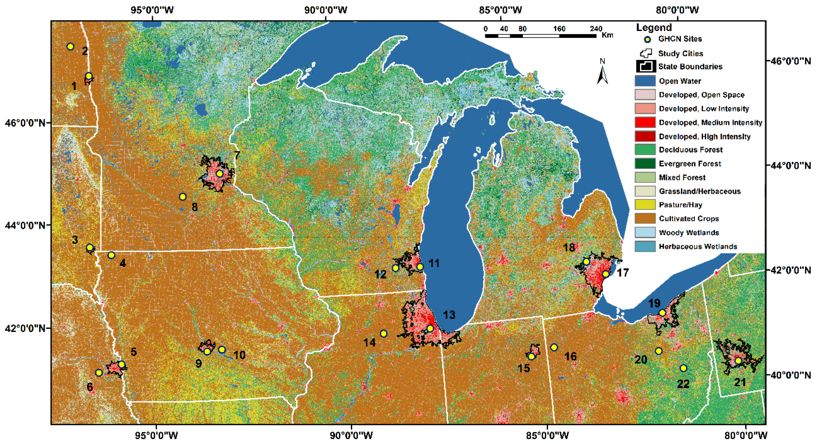
2.1. Study Region

Broadly known as the Upper Midwest, most of the region (78–98°W, 40–48°N) is located on a relatively flat, continental, temperate plain with no major mountain range. However, the U.S. Great Lakes in the northern and eastern ends of the region do present confounding meteorological influences for cities located on or near the Great Lakes. We selected the largest city in each state that is located within the bounds of our study region for a total of 11 cities (

Table 1. Eleven focal cities with population [37], urban extent [39], and population density from 2011 by metropolitan statistical area.

City	2011 Population (Total)	2011 Urban Extent (ha)	2011 Density (pop/ha)
Chicago	9,491,283	274,465	34.6
Detroit	4,287,556	152,077	28.2
Minneapolis-St. Paul	3,388,716	113,889	29.8
Pittsburgh	2,359,783	77,432	30.5
Cleveland	2,068,606	59,608	34.7
Milwaukee	1,561,108	47,261	33.0
Omaha	876,836	37,280	23.5
Des Moines	580,779	22,366	26.0
Fort Wayne	419,609	15,848	26.5
Sioux Falls	232,553	9468	24.6
Fargo	212,695	11,392	18.7

). Each focal city is embedded within a vegetated landscape and is relatively isolated from any other city. The cities range in population from ~0.2 M in Fargo, ND to ~9.5 M in the Chicago, IL metropolitan area [37]. A study of urban climate characterized the “ideal” conditions of UHIs arising from a city with a temperate climate, situated on flat terrain with population greater than 100,000 [11]. With the exception of Pittsburgh, PA, where terrain is relatively hilly, all of the focal cities match the “ideal” UHI criteria. Figure 1 shows the 2011 National Land Cover Database Land Cover Type data product with the eleven focal cities outlined in black [38]. The western and southern portions of the study region are predominantly crop and pasture lands (Figure 1, brown/yellow) compared with increasingly forested regions surrounding the cities to the north and east (Figure 1, shades of green).

2.2. Data

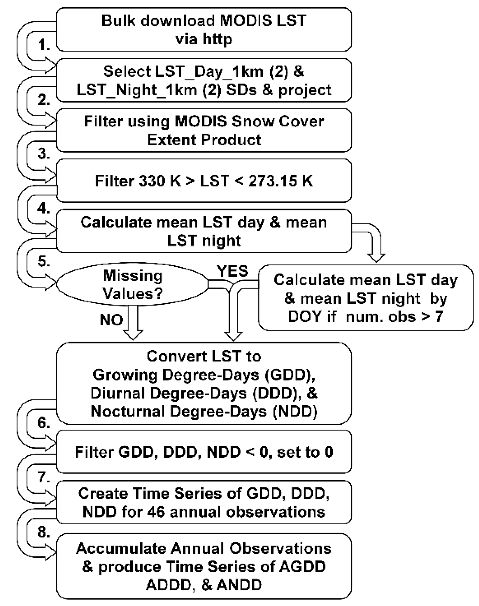
2.2.1. MODIS Land Surface Temperature

The Moderate-resolution Imaging Spectroradiometer (MODIS) is a scientific instrument aboard the NASA Earth Science satellites Aqua and Terra that operates as a part of the Earth Observing System [40,41]. Here, we used the MODIS-Aqua (MYD11A2) and MODIS-Terra (MOD11A2) products, which are level-3 global Land Surface Temperature and Emissivity 8-day composites at 1000 m resolution, provided in sinusoidal grid format as the mean clear-sky LST during an 8-day time frame [42]. The specific scientific datasets we used from the product include “LST_Day_1km” and “LST_Night_1km”, with units in Kelvin [42]. The overpass time for MODIS-Terra “LST_Day_1km” is 1030 local solar time and MODIS-Aqua is 1330 local solar time, and the overpass time for MODIS-Terra “LST_Night_1km” is 2230 local solar time and MODIS-Aqua is 0130 local solar time [43]. We obtained all M{Y|O}D11A2 observations from 2003 to 2012 (46 annually; 460 total) for MODIS tiles h10v04 and h11v04 [42]. We also downloaded the MODIS Aqua (MYD10A2) and Terra (MOD10A2) snow cover products, which contain level-3 global “Maximum Snow Extent” 8-day composites at 500 meter resolution [44].

2.2.2. Daymet Modeled Air Temperature

The Daymet data product provides daily mosaicked gridded estimates of weather parameters for North America [45]. The dataset is calculated from meteorological station observations via extrapolation and interpolation algorithms [45]. The Daymet data product is available as daily 1000 m resolution netCDF files, distributed in 2 degree × 2 degree tiles [45]. We downloaded the maximum and minimum air temperature products covering tiles 11,742–11,751, 11,922–11,929, 12,102–12,108, and 12,282–12,287 (31 tiles total) for years 2003–2012 [46]. The maximum and minimum air temperature parameters are described as the daily maximum and minimum 2-meter air temperature provided in degrees Celsius [45].

2.2.3. Global Historical Climatology Network

The Global Historical Climatology Network (GHCN) provides daily climate observations from ~30 weather station networks [47]. The network includes station-based measurements from more than 90,000 stations globally [47]. The dataset is reconstructed weekly and checked for quality assurance [47]. We used daily maximum and minimum temperature observations (tenths of degrees Celsius) provided by GHCN for 22 stations located in and nearby our study cities from 2003 to 2012 [48]. We selected one GHCN station within each of the eleven cities and an additional GHCN station located outside of each city (Figure 1). Information on the station names and geographic locations can be found in

Table 2. Global Historical Climatology Network study ID, city, type, station names, station ID, geographic location, and elevation [46]. Station ID numbers correspond to numbered labels found in Figure 1.

ID	City	Type	Station Name	Station ID	Lat	Lon	Elevation (m)
1	Fargo	U	Fargo Hector Intl. Airport	W00014914	46.9	−96.8	274
2	Fargo	R	Mayville	C00325660	47.5	−97.4	288
3	Sioux Falls	U	Sioux Falls Foss Field	W00014944	43.6	−96.8	435
4	Sioux Falls	R	Rock Rapids	C00137147	43.4	−96.2	412
5	Omaha	U	Omaha Eppley Airfield	W00014942	41.3	−95.9	299
6	Omaha	R	Mead 6 S	C00255362	41.1	−96.5	352
7	Minneapolis-St. Paul	U	University of Minn St. Paul	C00218450	45.0	−93.2	296
8	Minneapolis-St. Paul	R	Gaylord	C00213076	44.6	−94.2	310
9	Des Moines	U	Des Moines Intl. Airport	W00014933	41.5	−93.7	292
10	Des Moines	R	Neal Smith Iowa	R0000INEA	41.6	−93.3	274
11	Milwaukee	U	Milwaukee Mitchell Intl. Airport	W00014839	43.0	−87.9	204
12	Milwaukee	R	Milwaukee WSFO Dousman	C00478316	43.0	−88.5	284
13	Chicago	U	Chicago Midway Airport 3 SW	C00111577	41.7	−87.8	189
14	Chicago	R	Paw Paw 2 S	C00116661	41.7	−89.0	290
15	Fort Wayne	U	Fort Wayne Intl. Airport	W00014827	41.0	−85.2	252
16	Fort Wayne	R	Paulding	C00336465	41.1	−84.6	221
17	Detroit	U	Detroit City Airport	W00014822	42.4	−83.0	191
18	Detroit	R	White Lake 4 E	C00208941	42.7	−83.5	321
19	Cleveland	U	Cleveland Burke Lakefront Airport	W00004853	41.5	−81.7	178
20	Cleveland	R	Wooster Experimental Station	C00339312	40.8	−81.9	311
21	Pittsburgh	U	Pittsburgh Allegheny Co Airport	W00014762	40.4	−79.9	380
22	Pittsburgh	R	Dennison Water Works	C00332160	40.4	−81.3	262

.

2.3. Methods

2.3.1. Thermal Time

Our study used the MODIS LST, Daymet modeled air temperature, and GHCN air temperature observations in order to calculate three measures of thermal time. The Growing Degree-Day (GDD) measures the amount of heat available for plant development for a given calendar day [49]. In other words, the progress of calendar time is weighted by the daily temperature above a specific threshold: GDD is the maximum of either: (1) the average of the daily maximum (T_max) and minimum temperature (T_min) less the base temperature (T_base); or (2) zero, if the average falls below the base temperature (Equation (1)). Here we also introduce two new measures of thermal time that are constructed similarly to GDD—the Diurnal Degree-Day (DDD) and the Nocturnal Degree-Day (NDD). Whereas the GDD measures the amount of heat available for plant development using the average temperature for a given calendar day (e.g., the simple average of the daily maximum and minimum), DDD (or NDD) measures the amount of heat available during the daytime (or nighttime) associated with satellite overpass periods. Both DDD and NDD can accommodate one or more observations during the specified period, but here we used two daytime and nighttime land surface temperature observations, respectively. Constructed similarly to GDD, DDD (NDD) is the maximum of either: (1) the average land surface temperature from MODIS observations at 1030 (2230) and 1330 (0130) less the base temperature; or (2) zero if the average falls below the base temperature (Equations (2) and (3)). These times correspond to the nominal overpasses for the Terra and Aqua satellites, respectively. There is substantial variation in the exact overpass times, so it may be more appropriate to consider these periods as before noon and before midnight for Terra and after noon and after midnight for Aqua [50]. Moreover, while these overpass times will rarely coincide with the times of day for the temperature extremes, they are a relatively consistent temporal sample of the diel (24 h) temperature cycle. This study used a base temperature of 0 °C for all calculations of thermal time.

$$\text{GDD}= max\left\{\left[\frac{(T_{max}+T_{\text{min})}}{2}\right]-T_{base}, 0\right\}$$

(1)

$$\text{DDD}= max\left\{\left[\frac{(T_{day1}+T_{\text{day}2)}}{2}\right]-T_{base}, 0\right\}$$

(2)

$$\text{NDD}= max\left\{\left[\frac{(T_{night1}+T_{\text{night}2)}}{2}\right]-T_{base}, 0\right\}$$

(3)

We developed an algorithm to filter and convert MODIS LST into GDD, DDD, and NDD (Figure 2). We used the MODIS maximum snow extent product to exclude MODIS LST observations when snow cover was present. We resampled the 500 meter resolution MODIS maximum snow extent data to 1000 m using the nearest neighbor method provided by the Environment for Visualizing Images (ENVI) software in order to align each pixel with the corresponding MODIS LST 1000 m pixel. The MODIS LST observations were additionally filtered to exclude observations that were below freezing (273.15 K), or unreasonably high (330 K). Next, we converted the two daytime and two nighttime LST observations from Kelvin to degrees Celsius. The algorithm also calculates the mean daytime and nighttime LST for each 8-day compositing period (DOY) using the 10 observations (2003–2012) available for each DOY. The mean LST by DOY is only calculated when 8 or more years have available data. The decadal mean daytime and nighttime LST values are later used to fill data gaps where annual observations for a particular DOY have missing values. Next, the script calculates GDD, DDD, and NDD. GDD is calculated as the mean of the mean daytime (T₁₀₃₀ and T₁₃₃₀) and mean nighttime (T₂₂₃₀ and T₀₁₃₀) LST values, subtracted by a base of 0 °C (Equation (4)). DDD is calculated as the mean daytime LST (T₁₀₃₀ and T₁₃₃₀) and a base of 0 °C (Equation (5)). NDD is calculated as the mean nighttime LST (T₂₂₃₀ and T₀₁₃₀) and a base of 0 °C (Equation (6)).

$$\text{GDD}= max\left\{\left[\frac{\left(\text{mean}\left({\text{LST}}_{1030}+ {\text{LST}}_{1330}\right)+\text{mean}\left({\text{LST}}_{2230}+{\text{LST}}_{0130}\right)\right)}{2}\right]-T_{base}, 0\right\}$$

(4)

$$\text{DDD}= max\left\{\left[\frac{\left({\text{LST}}_{1030}+ {\text{LST}}_{1330}\right)}{2}\right]-T_{base}, 0\right\}$$

(5)

$$\text{NDD}= max\left\{\left[\frac{\left({\text{LST}}_{2230}+{\text{LST}}_{0130}\right)}{2}\right]-T_{base}, 0\right\}$$

(6)

The script filters the data to exclude observations where GDD, DDD, or NDD < 0, which signifies that zero Degree-Days (DD) were accumulated during that particular compositing period. The next step creates annual time series of GDD, DDD, and NDD multiplied by 8 to account for the 8-day compositing period of the MODIS products and accumulates each observation (DD in °C) by year. The final products are ten-year time series of Accumulated Growing Degree-Days (AGDD), Accumulated Diurnal Degree-Days (ADDD), and Accumulated Nocturnal Degree-Days (ANDD).

Both the Daymet and GHCN air temperature observations provide daily minimum and maximum temperature observations. Thus, the equations for calculating GDD, DDD, and NDD must differ slightly from the calculations tuned for MODIS LST data. GDD from both the Daymet and GHCN datasets is calculated as the mean daily temperature (T_max and T_min) subtracted by base 0 °C (Equation (7)). DDD (NDD) from both the Daymet and GHCN datasets is calculated as the daily maximum (minimum) temperature subtracted by base 0 °C (Equations (8) and (9)). To distinguish the difference between DDD and NDD calculated from the MODIS LST observations vs. the Daymet and GHCN air temperature observations, DDD and NDD calculated from Daymet and GHCN are referred to as “maxDD” and “minDD”, respectively.

$$\text{GDD}= max\left\{\left[\frac{\left({\mathrm{T}}_{\text{max}}+ {\mathrm{T}}_{\text{min}}\right)}{2}\right]-T_{base}, 0\right\}$$

(7)

$$\text{maxDD}= max\left\{T_{max}-T_{base}, 0\right\}$$

(8)

$$\text{minDD}= max\left\{T_{min}-T_{base}, 0\right\}$$

(9)

2.3.2. Dataset Comparison

To compare the derived thermal time series from the three different products, we calculated the decadal mean thermal time (GDD, DDD, and NDD) and accumulated thermal time (AGDD, ADDD, ANDD) for each dataset by DOY. We aggregated the daily Daymet and GHCN-derived measures to the 8-day compositing period of the MODIS LST-derived DD. This alignment provides the decadal mean GDD, DDD/maxDD, NDD/minDD, AGDD, ADDD/Accumulated T_max Degree-Days (AmaxDD), and ANDD/Accumulated T_min Degree-Days (AminDD) for 46 DOYs. We collected the time series data from the MODIS and Daymet-derived products for the 1000-m pixels where the corresponding 22 GHCN stations are located. We performed linear regression on the relationships between mean decadal DD by dataset for GDD, DDD, and NDD. We also used linear regression to characterize the relationships between each urban and rural station pair to evaluate the ability of each dataset to capture the UHI effect. We analyzed the evolution of the UHI over the course of a year and the differences between urban versus rural and daytime versus nighttime dynamics.

3. Results

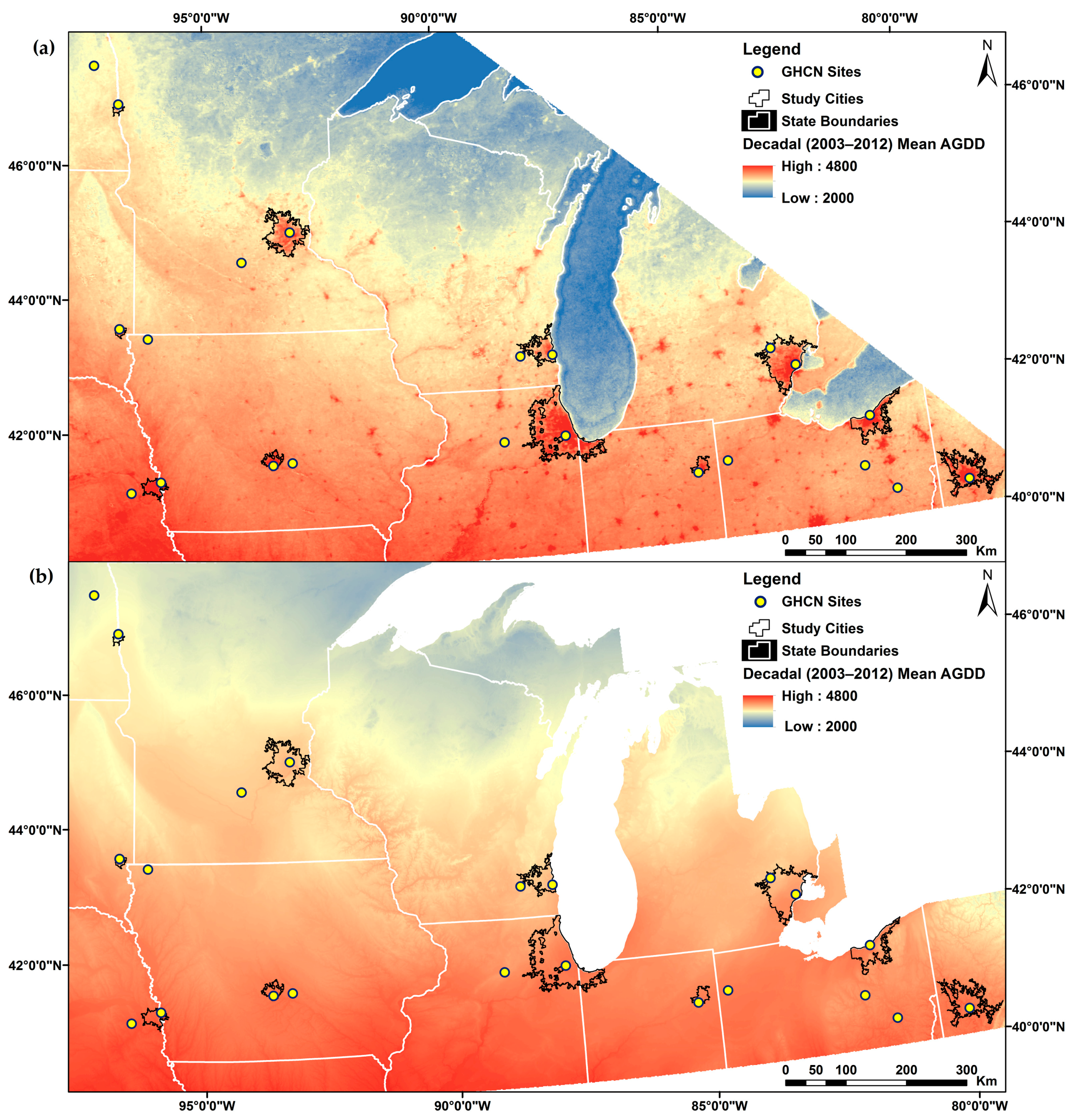
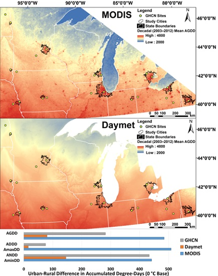
3.1. Regional Characterization of Thermal Regimes

3.1.1. AGDD

Figure 3 shows the decadal (2003–2012) mean total Accumulated Growing Degree-Days over the Upper Midwest as produced using the (a) MODIS and (b) Daymet temperature observations. On a regional scale, the dominant spatial pattern in AGDD is similar when comparing the results from MODIS with those from Daymet. The thermal gradient from southwest to northeast can be seen in both images, where shades of red (blue) indicate higher (lower) AGDD. Daymet results appear smoother with less fine-scale spatial detail than MODIS results. Major river valleys have higher annual AGDD in the results from both datasets. Three of the major river valleys in the Upper Midwest include from west to east: the Missouri River (forming the border between Nebraska and Iowa), the Mississippi River (forming the eastern border of Iowa), and the Illinois River (flowing through central Illinois), and these low-lying river valleys experience higher AGDD than the surrounding areas.

Two major differences are evident between AGDD derived from MODIS land surface temperature and AGDD derived from Daymet modeled air temperature observations. The first and more obvious difference is that Daymet data do not include air temperature over the Great Lakes. The Great Lakes have low AGDD as seen from the MODIS LST-derived results, appearing in shades of blue in Figure 3. Lake Superior has the lowest total AGDD of the study region. Lake Superior is both the deepest and most northerly Great Lake. Located in the center of the region in north-south orientation is Lake Michigan, and farthest east is Lake Erie. Moving farther south in both Lake Michigan and Lake Erie increases the annual AGDD. Lake Erie is the shallowest Great Lake, and the western end of Lake Erie (south of Detroit) is much shallower than Lakes Michigan and Superior; consequently, it shows a much higher annual AGDD in shades of tan.

The second major difference between the AGDD results from MODIS and Daymet is the appearance of local “hotspots” (as shades of red) in the MODIS AGDD (Figure 3a) but not the Daymet AGDD (Figure 3b). The phenomenon is particularly evident in the focal cities of the study region that are outlined in black. Even much smaller cities appear as small “hotspots” throughout the region. In contrast, it is very difficult to distinguish urban from rural areas in the Daymet results (Figure 3b).

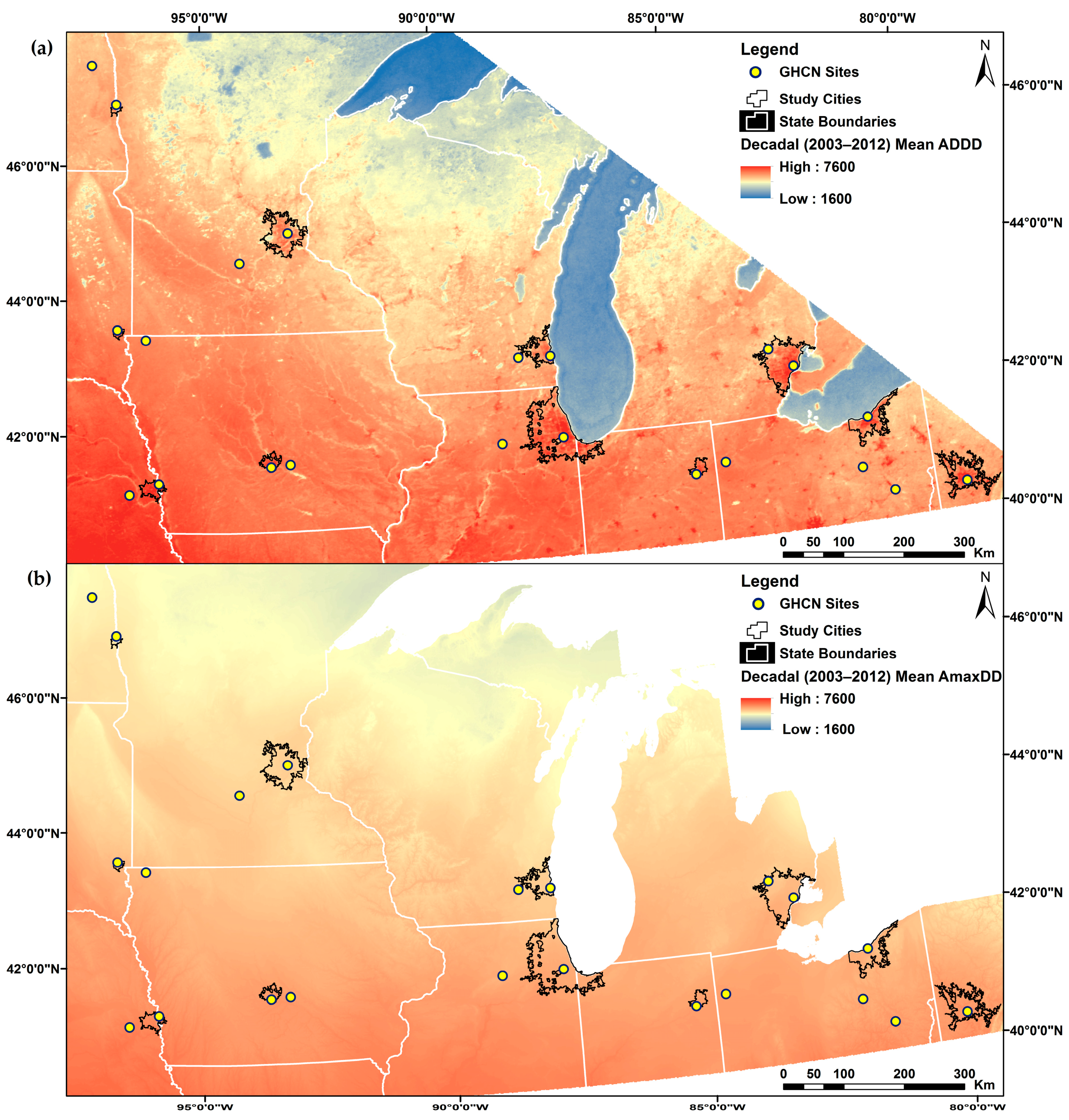
3.1.2. ADDD and AmaxDD

Figure 4 shows the decadal (2003–2012) mean Accumulated Diurnal Degree-Days over the Upper Midwest produced from the (Figure 4a) MODIS LST observations and the decadal (2003–2012) mean Accumulated maximum Degree-Days produced using the (Figure 4b) Daymet air temperature data. The dominant spatial pattern in ADDD/AmaxDD is similar at the regional scale in both sets of results. A gradient from southwest to northeast can be seen in both images. However, the range in Degree-Days from the MODIS results is much greater than in the Daymet results. The dynamic range in the MODIS results is very large, ranging from 1600 ADDD over northern Lake Superior to 7600 in southern Nebraska (Figure 4a). A lower range is evident in the Daymet (Figure 4b), where there is very little contrast, as most of the region appears in a similar shade of light red to tan in color. Again, the Daymet results appear smoother than the MODIS. Major river valleys have higher annual AmaxDD, but they appear lower in ADDD than the surrounding areas.

The Great Lakes have low ADDD, appearing in shades of blue. Similarly, smaller inland lakes also appear to have lower ADDD in the MODIS results, including Lake Mille Lacs north of the Minneapolis-St. Paul, MN region and Lake Winnebago north of Milwaukee, WI (Figure 4a). However, the Daymet results do not show lower AmaxDD over either of these large inland lakes (Figure 4b). Variations in ADDD also appear to be influenced by land cover. In the southern and western portions of the region, ADDD is higher (crop and pasturelands, Figure 1) while the northern and eastern portions of the region have lower ADDD (forests and wetlands, Figure 1). In the MODIS LST-derived results (Figure 4a), cities again appear as local “hotspots” (shades of red) compared to the surrounding rural landscape, although the contrast is less striking than in the AGDD (Figure 3a). Again, it is very difficult to distinguish urban from rural areas with the mean annual AmaxDD derived from Daymet air temperature data (Figure 4b).

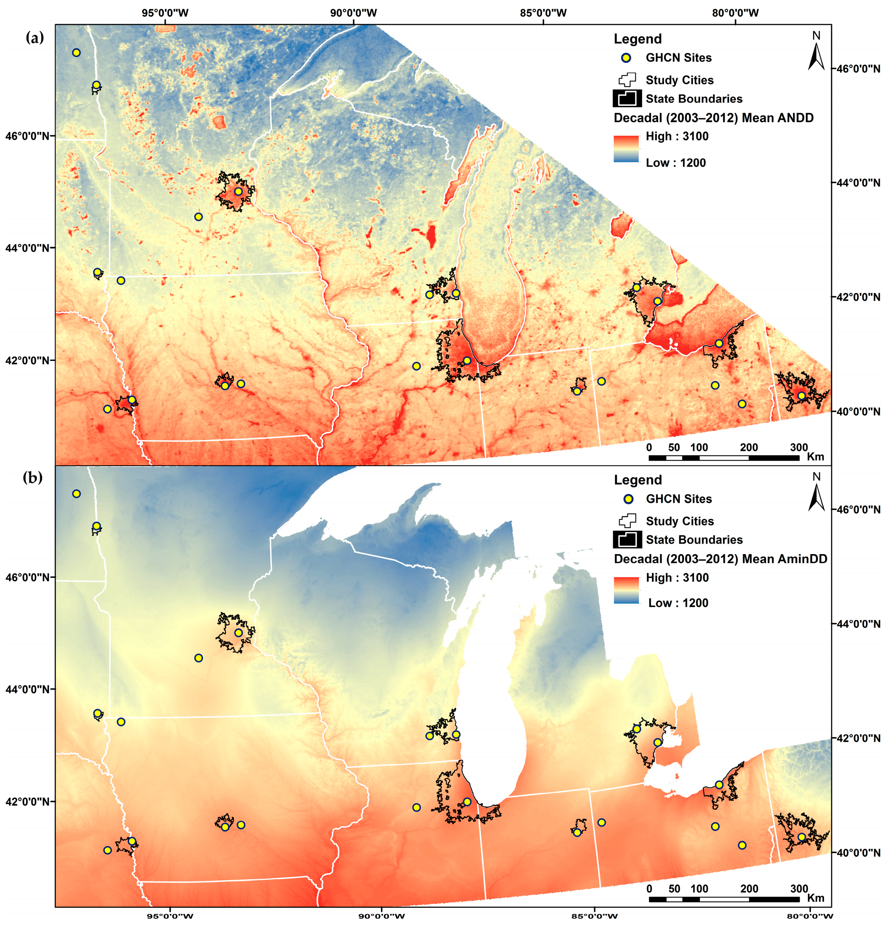
3.1.3. ANDD and AminDD

Figure 5 shows the decadal (2003–2012) mean Accumulated Nocturnal Degree-Days over the Upper Midwest as produced using the (a) MODIS data and the decadal (2003–2012) mean Accumulated minimum Degree-Days produced using the (b) Daymet data. The dominant spatial pattern in ANDD/AminDD is similar at the regional scale in both sets of results. However, the thermal gradient from southwest to northeast seen with AGDD and ADDD/AmaxDD has shifted to predominantly north–south. The regional ranges of ANDD and AminDD are much smaller compared to AGDD and ADDD/AmaxDD. Daymet results again appear smooth with less detail than the MODIS results. Major river valleys have higher annual ANDD (Figure 5a) and higher AminDD (Figure 5b) than the surrounding regions.

The Great Lakes have generally higher ANDD than the surrounding land. The difference in the physical characteristics of the different Great Lakes once again becomes evident: the shallower Lake Erie located farther south exhibits higher ANDD while the deeper, northern reaches of Lake Superior retain relatively low ANDD (Figure 5a). Smaller inland lakes also appear with higher ANDD, including the numerous lakes north of the Minneapolis-St. Paul, MN region and Lake Winnebago north of Milwaukee, WI (Figure 5a). Although the Daymet AminDD map shows a local “hotspot” over Lake Winnebago (Figure 5b), it is difficult to detect thermal anomalies for most inland lakes in the Daymet data (Figure 5b). Areas surrounding the Great Lakes have higher AminDD than regions farther away, and this phenomenon can be seen in both urban and rural areas (Figure 5b). In the ANDD map (Figure 5a), cities again appear as local “hotspots”. In the AminDD map (Figure 5b), the larger urban areas do show some contrast with the surrounding landscape, notably in Minneapolis-St. Paul, MN and Chicago, IL.

3.2. Urban/Rural Differences and Dataset Comparison

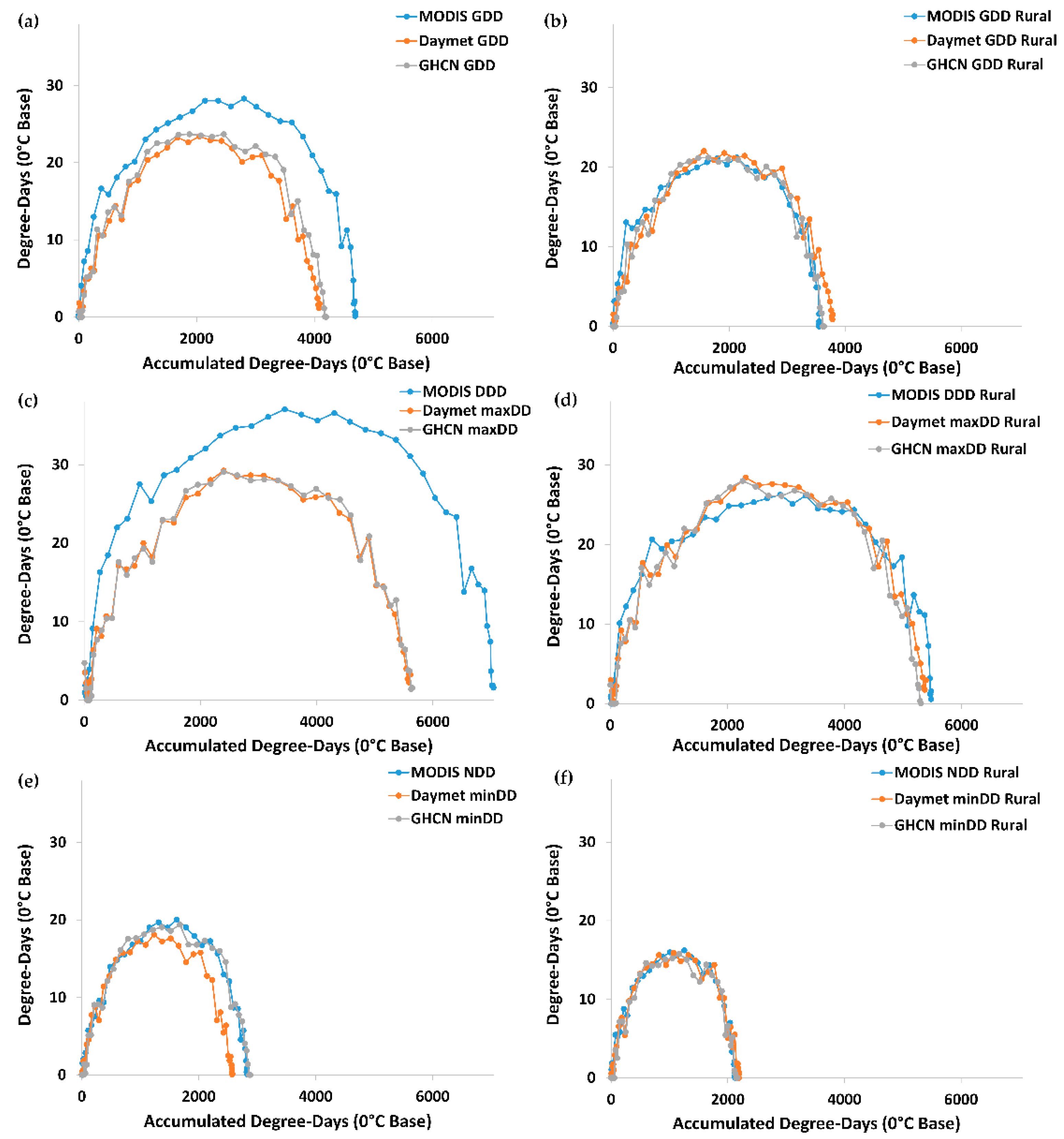
3.2.1. Urban/Rural Differences in Thermal Time

We compared the decadal (2003–2012) mean of thermal time (GDD, DDD/maxDD, and NDD/minDD) by day of year to identify urban/rural differences in thermal time and the differences between the three datasets.

Table 3. Different combinations of datasets, metrics of thermal time, and urban/rural comparisons with corresponding root mean square difference (RMSD) and Spearman correlation coefficient from linear regression analyses between thermal time derived from MODIS, Daymet, and GHCN.

X	Y	RMSD	Spearman Coefficient
Daymet GDD Rural	Daymet GDD	0.31	0.997
Daymet NDD Rural	Daymet NDD	0.37	0.995
Daymet DDD Rural	Daymet DDD	0.41	0.997
GHCN GDD	Daymet GDD	0.70	0.987
MODIS NDD Rural	MODIS NDD	0.71	0.986
GHCN DDD	Daymet DDD	0.72	0.992
GHCN NDD	Daymet NDD	0.73	0.975
GHCN GDD Rural	GHCN GDD	0.79	0.993
Daymet NDD Rural	MODIS NDD Rural	0.82	0.980
GHCN NDD Rural	Daymet NDD Rural	0.84	0.961
GHCN NDD Rural	GHCN NDD	0.90	0.983
Daymet NDD	MODIS NDD	0.93	0.983
GHCN GDD Rural	Daymet GDD Rural	0.94	0.983
GHCN NDD Rural	MODIS NDD Rural	0.97	0.961
GHCN NDD	MODIS NDD	1.01	0.974
GHCN DDD Rural	GHCN DDD	1.07	0.989
GHCN DDD Rural	Daymet DDD Rural	1.13	0.986
MODIS GDD Rural	MODIS GDD	1.20	0.982
GHCN GDD	MODIS GDD	1.66	0.982
Daymet GDD	MODIS GDD	1.70	0.978
MODIS DDD Rural	MODIS DDD	1.73	0.968
Daymet GDD Rural	MODIS GDD Rural	1.85	0.971
GHCN GDD Rural	MODIS GDD Rural	1.90	0.970
Daymet DDD	MODIS DDD	2.62	0.967
GHCN DDD	MODIS DDD	2.68	0.965
Daymet DDD Rural	MODIS DDD Rural	3.03	0.935
GHCN DDD Rural	MODIS DDD Rural	3.21	0.927

summarizes the results from linear regression analysis. All relationships were statistically significant with coefficients of determination ranging from 0.86–0.98. The root mean square difference (RMSD) was lowest for the relationship between urban and rural Daymet GDD with a correspondingly high correlation between the GDD calculated from Daymet at urban sites and the GDD calculated from Daymet at rural sites. Daymet urban vs. rural comparisons showed the highest correlation for all three metrics of thermal time (GDD, maxDD, and minDD; RMSD = 0.31–0.41). Metrics of thermal time taken from the urban sites between GHCN and Daymet also showed high correlations. However, between GHCN urban and rural metrics of thermal time RMSD ranged from 0.79–1.07. The RMSD between MODIS urban and rural metrics of thermal time ranged from 0.71–1.73. The weakest correlation for GHCN urban/rural values was at night (minDD); in contrast, the weakest correlation was during the daytime (DDD) for MODIS urban/rural values.

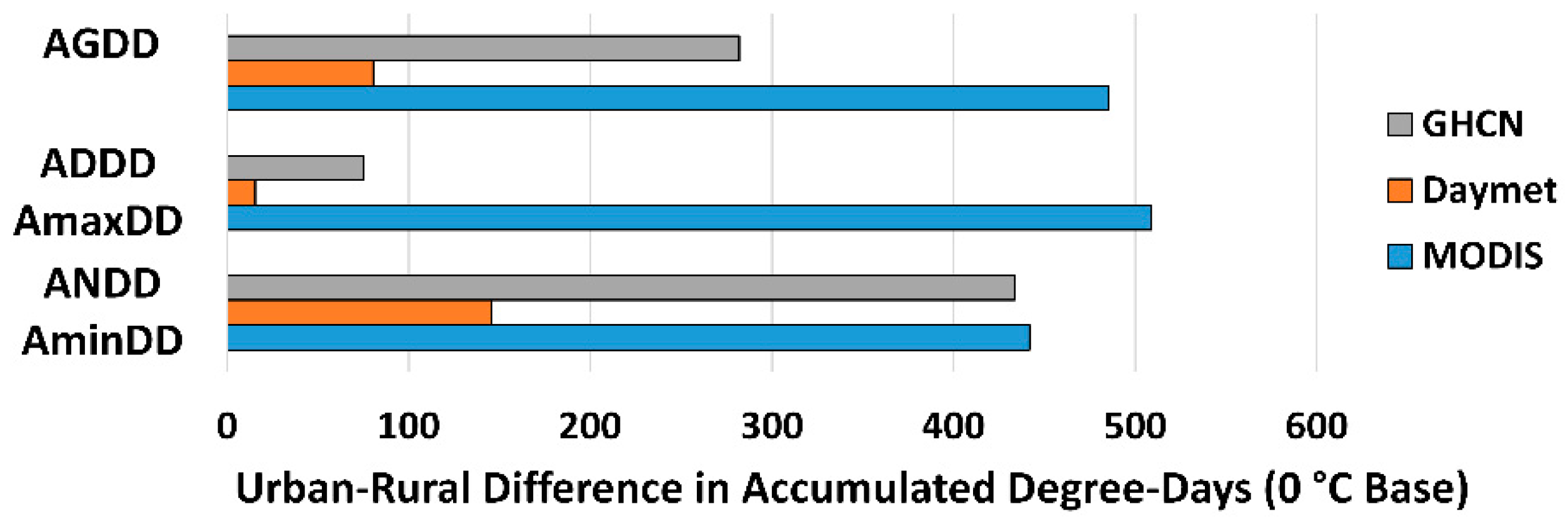
3.2.2. Urban/Rural Differences in Accumulated Thermal Time

We used the 11 urban and rural station pairs from the Global Historical Climatology Network (Table 2) and corresponding pixels from Daymet and MODIS to analyze urban/rural differences in thermal time and to compare the results from each dataset. Figure 6 shows the mean urban–rural difference in AGDD, ADDD, and ANDD. Values represented in Figure 6 were calculated as the mean urban–rural difference in decadal mean annual accumulated thermal time (AGDD, ADDD or AmaxDD, and ANDD or AminDD) from the eleven urban/rural station pairs. The urban–rural differences in all three accumulated thermal time metrics were highest from the MODIS LST-derived results (Figure 6, blue). The difference was greatest in ADDD and least in ANDD. In contrast, Daymet consistently had the lowest urban–rural differences for all three metrics (Figure 6, orange). The urban–rural differences in accumulated thermal time from the GHCN station air temperature data showed the greatest difference in AminDD, followed by AGDD, and the smallest urban–rural difference in AmaxDD (Figure 6, grey). MODIS results were much closer to GHCN results than Daymet during nighttime; whereas, Daymet results were much closer to GHCN results than MODIS during daytime. The urban–rural differences in AGDD derived from GHCN station data were between the differences from Daymet (lower) and MODIS (higher).

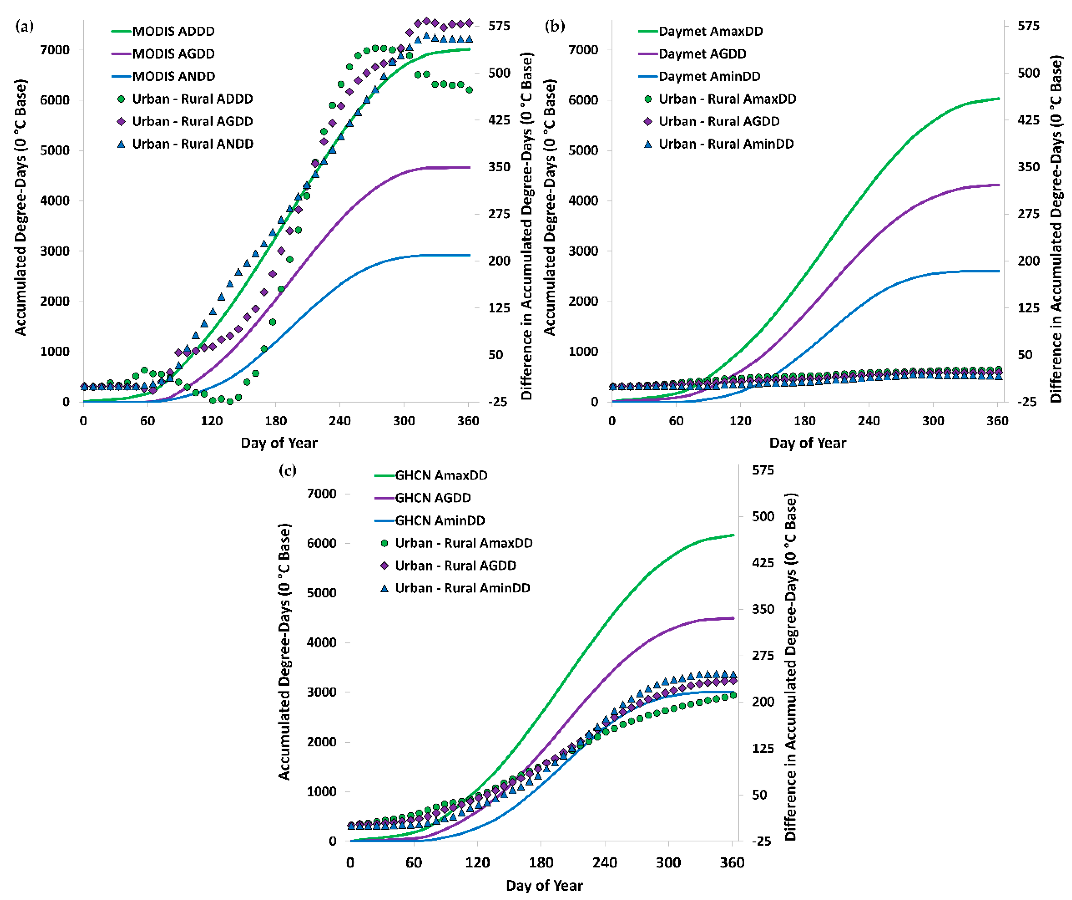
3.2.3. Seasonal Progression of Urban/Rural Differences in Accumulated Thermal Time

Figure 7 shows the decadal (2003–2012) mean AGDD, ADDD/AmaxDD, and ANDD/AminDD by day of year (46 dates representing the 46 8-day compositing periods of the MODIS data) for the urban GHCN station in Des Moines, IA (ID = 9, Table 2). In general, ADDD (or AmaxDD) is the highest metric of accumulated thermal time (Figure 7, green), followed by AGDD (purple), and lowest is ANDD (or AminDD, blue). Based on the accumulation curves in Figure 7, the seasonal progression of thermal time at this location is evident: in the winter months when temperatures are below freezing (0 °C), the line is flat; a steep slope of rapid warming occurs during the late spring and summer months; and the pace of thermal accumulation slows as autumn gives way to freezing conditions near year’s end (Figure 7). The symbols shown in Figure 7 trace the seasonal progression of urban–rural differences in AGDD, ADDD/AmaxDD, and ANDD/AminDD. Notice the large urban–rural differences in accumulated thermal time from MODIS (Figure 7a; 2nd y-axis) followed by GHCN (Figure 7c; 2nd y-axis), and the very small urban–rural differences in accumulated thermal time from Daymet (Figure 7b; 2nd y-axis). These patterns align with the results displayed in Figure 3b, Figure 4b and Figure 5b, where it was difficult to distinguish urban areas from the surrounding rural regions using Daymet data.

Urban–rural differences in accumulated thermal time were not evenly distributed throughout the year. The most dynamic seasonal difference occurred in the MODIS urban–rural ADDD difference (Figure 7a; green circles). The difference was higher in the early spring before decreasing and actually became negative for a portion of the spring season. The urban–rural difference in ADDD then increased rapidly before peaking again near the height of summer, and by the end of the year the urban–rural difference in ADDD decreased and was lower than the urban–rural difference in AGDD (purple diamonds) and ANDD (blue triangles). The results from the GHCN air temperature-derived thermal time were similar to those from MODIS, where AmaxDD was higher than AGDD or AminDD during the early spring, but by the end of the year was lower than AGDD and AminDD (Figure 7c). However, the urban–rural differences in accumulated thermal time from GHCN did not include the peaks and troughs evident in the urban–rural differences of ADDD from MODIS.

3.2.4. Thermal Time versus Accumulated Thermal Time

Figure 8 shows decadal mean thermal time (GDD, DDD/maxDD, and NDD/minDD) versus accumulated thermal time (AGDD, ADDD/AmaxDD, and ANDD/AminDD) derived from MODIS (blue), Daymet (orange), and GHCN (grey) data for the Detroit, MI urban (ID = 17, Table 2) and rural (ID = 18, Table 2) sites. Observations for the urban site (Figure 8a,c,e) had generally higher thermal time and accumulated thermal time than the rural site (Figure 8b,d,f). This discrepancy indicates a potentially longer growing season within the city of Detroit, MI, compared to the surrounding rural areas. The urban–rural difference was strongest in DDD from MODIS (Figure 8c,d; blue). Figure 8a,c shows that both the thermal time and accumulated thermal time are higher than the thermal time and accumulated thermal time derived from Daymet and GHCN air temperature observations. However, in terms of NDD/ANDD (Figure 8e) the results from MODIS are closer to the results from GHCN compared with the Daymet modeled air temperature-derived minDD and AminDD. The results from the rural site (Figure 8b,d,f) show little variation between the thermal time and accumulated thermal time derived from MODIS LST, Daymet modeled air temperature, or GHCN air temperature observations. Figure 8 also shows the distinct seasonality driven by the annual cycle of insolation that is characteristic of the temperate northern climate of the study region [51], and all relationships in Figure 8 fit a statistically significant convex quadratic regression model with coefficients of determination between 0.89–0.96.

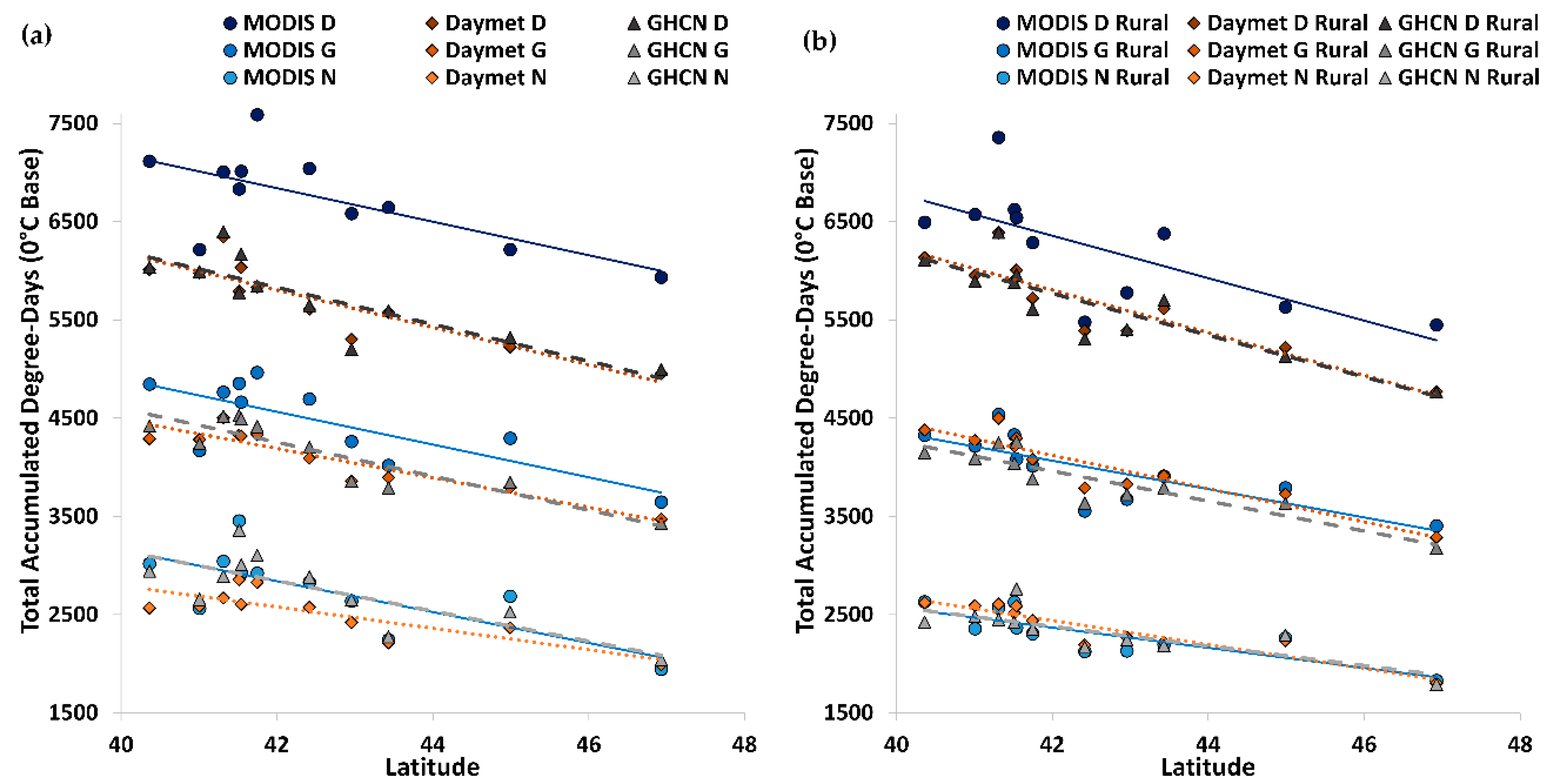
3.2.5. Latitudinal Effects

Although our study region spans only eight degrees latitude (40–48 °N), the region experiences considerable latitudinal influence on the local thermal regime. Figure 9 shows mean decadal (2003–2012) total accumulated thermal time (AGDD, ADDD/AmaxDD, and ANDD/AminDD) versus latitude from MODIS (shades of blue), Daymet (shades of orange), and GHCN (shades of grey) for all eleven (Figure 9a) urban and (Figure 9b) rural study sites. A statistically significant negative linear relationship between total accumulated DD and latitude was found for all cases, with coefficients of determination ranging from 0.47–0.86. Thus, it is evident that latitude affects the accumulated thermal time in the study region. We also performed a multiple analysis of covariance test (ANCOVA), and found that only the slope for MODIS DDD from the rural sites was significantly different from the slopes for the GHCN and MODIS NDD from the rural sites. All other combinations were not significantly different for the fitted slope parameter coefficient.

4. Discussion

The results from the spatial analysis of decadal mean accumulated thermal time metrics, including Accumulated Growing Degree-Days (AGDD), Accumulated Diurnal Degree-Days (ADDD), and Accumulated Nocturnal Degree-Days (ANDD) were different depending on dataset, and consequently the type of temperature being measured. MODIS LST results showed urban areas appearing as local “hot spots” for all three metrics; whereas, the Daymet air temperature results revealed urban hotspots only for AminDD, and then for only the largest cities. Daymet modeling of air temperature data does not account for urban microclimatic effects—namely the Urban Heat Island. This conclusion is further supported by the linear regression analyses, where Daymet urban versus rural Growing Degree-Days (GDD), maximum Degree-Days (maxDD), and minimum Degree-Days (minDD) have the three lowest RMSD values, nearly half of the RMSD values for the GHCN and MODIS urban–rural differences. This pattern indicates that urban areas do not influence local temperature observations as calculated from Daymet modeled air temperature data. Figure 6 shows the very small urban–rural differences in the three measures of accumulated time as calculated by Daymet (orange), where the urban–rural differences are less than half of the urban–rural differences as calculated from the GHCN air temperature station observation data. In particular, the Daymet data appear to underestimate the UHI effect of smaller cities, which can be seen in Figure 7b, where total urban–rural differences in accumulated thermal time for Des Moines, IA are less than 50 Accumulated Degree-Days for all three metrics, compared to the MODIS results, where urban–rural differences exceed 450 Accumulated Degree-Days in all cases, and GHCN, where urban–rural differences range between 200–275 Accumulated Degree-Days.

Another interesting finding from the linear regression analyses between urban/rural Degree-Days is that the RMSD of the MODIS results ranges from 0.71–1.73, similar to the results from GHCN (0.79–1.07). However, upon further inspection, the RMSD for MODIS urban versus MODIS rural DDD is higher than for GDD or NDD (1.73) while the RMSD for GHCN urban versus GHCN rural minDD is higher than GDD or maxDD. This pattern indicates that urban–rural differences in LST are greatest during the day (DDD) compared to urban–rural differences in air temperature, which are greatest at night (minDD). These results make sense in the context of differences between surface urban heat islands (SUHI) that are characterized by land surface temperature observations and the more traditional urban heat islands (UHI) that are measured by air temperature observations. Under stable conditions, the air temperature UHI is most pronounced during the overnight hours as a result of reduced cooling rates from late afternoon into the evening [6,18,19]. In contrast, the land surface temperature SUHI is more intense near midday compared to night, because surfaces heat and cool faster than air [32]. One modeling study of major US cities found that maximum differences in urban/rural LST occur near 1100 [36]. Their finding helps to explain why the greatest urban–rural differences in Accumulated Degree-Days occurs for Accumulated Nocturnal Degree-Days for the two air temperature datasets (Daymet, GHCN) compared to the MODIS LST dataset where urban–rural differences are greatest as measured using Accumulated Diurnal Degree-Days (Figure 6). It is worth mentioning again that the overpass time for MODIS-Terra “LST_Day_1km” is 1030 local solar time and MODIS-Aqua is 1330 local solar time, which is during the peak timing of urban–rural LST differences. Studies have also found that LST is generally higher than corresponding air temperatures, which helps to explain the major differences in both AGDD versus GDD and ADDD versus DDD found for the urban Detroit, MI site (Figure 8a,c). One study using MODIS LST in Milan, Italy found daytime SUHI intensity to peak between 9 K and 10 K, decreasing by a factor of two at night [52]. Interestingly, while the results from MODIS appear significantly higher for (A)GDD and (A)DDD, the results from MODIS LST-derived (A)NDD are actually closer to the GHCN station data compared to the Daymet modeled air temperature-derived results (Figure 8e). For the rural Detroit, MI site, all three datasets show similar results for all three thermal time metrics (Figure 8b,d,f).

Over the course of a year, urban–rural differences in accumulated thermal time are striking. In particular, the urban–rural difference in MODIS LST-derived results during the day (ADDD) change drastically over the progression of a year (Figure 7a), because LST is strongly influenced by land cover/land use, including impervious surface area [19,32,53]. The seasonality of urban–rural differences in ADDD is important in the Upper Midwest of the United States because: (1) the temperate climate drives land surface phenology; and (2) the rural vegetated land surface changes drastically over the course of the year. Croplands of the region typically have bare soil in spring, followed by dense, green vegetation during the summer, and ultimately dried out crops and crop residue following the harvest in fall. Broadleaf forests are bare in the spring, followed by dense foliage during the summer, and ultimately senesce and drop leaves in the fall. Land surface phenology helps to explain our understanding of Figure 7a, where urban–rural differences hover near zero in the winter, since neither urban nor rural locations are accumulating any thermal time when temperatures are below the base temperature threshold. By early spring, there is a small peak in the urban–rural difference in ADDD, suggesting that urban areas begin to thaw from the cold winter faster than corresponding rural areas. However, as spring progresses, urban–rural ADDD differences decrease and actually fall below zero for a short period (indicating warmer land surface temperatures in rural areas). This phenomenon is likely due to the increased extent of bare soils in rural areas (lack of crops, trees yet to have foliage) compared to urban areas; studies have found earlier green-up in cities compared to corresponding rural areas [6,54,55]. As spring gives way to summer, the rural crop and tree canopies quickly develop, and urban–rural differences in ADDD increase rapidly, until the difference peaks near the end of summer. This period is characterized by full vegetation canopy and the hottest temperatures of the year. The transpiring vegetation covering the rural areas leads to lower temperatures than the drier, hotter impervious surfaces throughout urban areas. As summer gives way to fall, urban–rural differences in ADDD begin to decrease because the crop canopy dries and is eventually harvested, and the tree canopy senesces and drops leaf, in combination with urban areas where vegetation remains greener for longer, due to increased duration of the growing season [51].

In situ air temperature observations span a longer record and have a higher temporal resolution, but suffer from poor spatial coverage [29]. The advent of satellite remote sensing in the 1970s created new opportunities to measure and monitor urban areas, and more specifically, urban heat islands. Satellite derived thermal infrared data is useful for assessing urban climatic characteristics because it provides complete spatial coverage over urban areas when compared to in situ air temperature data [29]. However, satellite-derived land surface temperature data are constrained to a shorter climatological record and suffer from lower temporal resolution [29]. Also, urban thermal climate studies must account for inherent differences between air temperature and land surface temperature data. This study provides insight into the differences between more traditional urban heat island monitoring using air temperature observations, and the surface urban heat island that is monitored using land surface temperature observations from satellite remote sensors. Our results show similarities and differences between MODIS LST-derived and Daymet modeled air temperature-derived measures of thermal time and accumulated thermal time, and ultimately how they compare to corresponding GHCN station observations of air temperature. However, as is always the case when dealing with remote sensing observations, we are constrained by our temporal resolution (46 annual 8-day composites) and missing data due to snow and cloud cover. By leveraging a decade of observations, we have obtained greater confidence in the observed differences in thermal time.

We have provided an overall assessment of urban–rural differences in daily, daytime, and nighttime thermal time as seen through MODIS land surface temperature observations, Daymet modeled air temperature estimates, and GHCN station air temperature observations for eleven cities in the Upper Midwest of the United States. Our results would likely differ in parts of the country with very different climate, i.e., in the arid Southwest. We know from past studies that UHI/SUHI dynamics vary by biome [19]. Moreover, land surface temperature observations are influenced by land use, land cover, and land condition, including the land surface phenology; thus, the MODIS observations that capture conditions at particular times of day will likely differ from the daily temperature extremes. Future research could investigate the influence of impervious surface area, land cover type, elevation, proximity to water bodies, and other land surface variables that could influence the microclimatic texture of the UHI/SUHI. However, the complex fabric of urban areas often leads to mixtures of materials within pixels [56]. The locations of weather stations and the composition of nearby urban (or rural) surfaces can also affect observed temperatures. We recognize the limitation of comparing in situ air temperature observations at a point with the coarser resolution land surface temperature observations. To better compare point-source station observations with the MODIS/Daymet 1000 m resolution data and decrease the influence of mixed pixels, future research could use downscaling techniques to increase spatial resolution, which has been done down to 100 m resolution for urban LST observations [57]. To further explore local spatial microclimatic differences within cities, future studies could aim to analyze not only urban–rural differences in thermal time, but also differences within cities and the surrounding peri-urban to rural environments using the Local Climate Zones approach [58]. Spatial resolution of available thermal remote sensing data is a limitation.

5. Conclusions

This study demonstrates the differences and similarities between datasets measuring air temperature and land surface temperature, and their application of and subsequent implications on studies of urban climate. The first key finding of this study is that the Daymet modeled daily temperature estimates do a poor job of accounting for UHI-induced amplification of urban temperatures, and exhibit very small urban–rural temperature differences, even after accumulating the thermal time over the course of a year. The second key finding is that MODIS LST-derived differences in urban–rural thermal time are much greater than the corresponding weather station air temperature-derived metrics during the daytime (diurnal); however, the nighttime (nocturnal) dynamics of thermal time between both datasets are quite similar. Major differences in daytime characterization of UHIs arise from differences in the object being measured. That is, characterization of UHIs using air temperature observations is measuring a different urban thermal climate phenomenon than are land surface temperature observations, which characterize the surface UHI. The SUHI show more seasonal dynamics than the UHI, due to the physical differences of urban and rural land covers that are amplified by differences in urban and rural land surface phenologies [59]. This information should prove useful to inform a variety of interests, including scientists interested in performing urban thermal climate analyses as well as urban land surface modelers, urban ecologists, urban planners, urban developers, urban policy-makers, meteorologists, and climatologists.

References

1. United Nations. World Urbanization Prospects: The 2014 Revision, Highlights. Department of Economic and Social Affairs, Population Division 2014, (ST/ESA/SER.A/352). Available online: http://esa.un.org/unpd/wup/highlights/wup2014-highlights.pdf (accessed on 20 January 2016).
2. Seto, K.C.; Fragkias, M.; Güneralp, B.; Reilly, M.K. A meta-analysis of global urban land expansion. PLOS ONE 2011, 6, 1–9. [Google Scholar] [CrossRef] [PubMed]
3. Angel, S.; Parent, J.; Civco, D.L.; Blei, A.M. Making Room for a Planet of Cities; Lincoln Inst. of Land Policy: Cambridge, MA, USA, 2011. [Google Scholar]
4. Seto, K.C. Global urban issues: A primer. In Global Mapping of Human Settlement: Experiences, Datasets, and Prospect; Gamba, P., Herold, M., Eds.; Taylor and Francis Group: CRC Press: Boca Raton, FL, USA, 2009; pp. 3–9. [Google Scholar]
5. Arnfield, J. Two decades of urban climate research: A review of turbulence exchanges of energy and water, and the urban heat island. Int. J. Clim. 2003, 80, 386–395. [Google Scholar] [CrossRef]
6. Oke, T.R. Boundary Layer Climates, 2nd ed.; Methuen & Co.: London, UK, 1987. [Google Scholar]
7. Voogt, J.A. Urban heat island. In Encyclopedia of Global Environmental Change; John Wiley & Sons: New York, NY, USA, 2002; pp. 660–666. [Google Scholar]
8. McCarthy, M.P.; Best, M.J.; Betts, R.A. Climate change in cities due to global warming and urban effects. Geophys. Res. Lett. 2010, 37, 1–5. [Google Scholar] [CrossRef]
9. Changnon, S.A.; Kunkel, K.E.; Reinke, B.C. Impacts and responses to the 1995 heat wave: A call to action. Bull. Am. Meteorol. Soc. 1996, 77, 1497–1506. [Google Scholar] [CrossRef]
10. Patz, J.A.; Campbell, D.; Holloway, T.; Foley, J.A. Impact of regional climate change on human health. Nature 2005, 438, 310–317. [Google Scholar] [CrossRef] [PubMed]
11. Oke, T.R. The energetic basis of the urban heat island. Q. J. R. Meteorol. Soc. 1982, 108, 1–24. [Google Scholar] [CrossRef]
12. Avissar, M. The effects of urban patterns on ecosystem function. Int. Regional Sci. Rev. 2005, 28, 168–192. [Google Scholar]
13. Lo, C.P.; Quattrochi, D.A. Land-use and land-cover change, urban heat island phenomenon, and health implications: A remote sensing approach. Photogramm. Eng. Remote Sens. 2003, 69, 1053–1063. [Google Scholar] [CrossRef]
14. Chen, X.; Zhao, H.; Li, P.; Yin, Z. Remote sensing image-based analysis of the relationship between urban heat island and land use/cover changes. Remote Sens. Environ. 2006, 104, 133–146. [Google Scholar] [CrossRef]
15. Hartmann, D.L.; Klein Tank, A.M.G.; Rusticucci, M.; Alexander, L.V.; Brönnimann, S.; Charabi, Y.; Dentener, F.J.; Dlugokencky, E.J.; Easterling, D.R.; Kaplan, A.; et al. Observations: Atmosphere and Surface. In Climate Change 2013: The Physical Science Basis, Contribution of Working Group I to the Fifth Assessment Report of the Intergovernmental Panel on Climate Change; Stocker, T.F., Qin, D., Plattner, G.K., Tignor, M., Allen, S.K., Boschung, J., Nauels, A., Xia, Y., Bex, V., Midgley, P.M., Eds.; Cambridge University Press: Cambridge, UK; New York, NY, USA, 2013; pp. 161–218. [Google Scholar]
16. Oke, T.R.; Johnson, G.T.; Steyn, D.G.; Watson, I.D. Simulation of nocturnal surface urban heat islands under “ideal” conditions: Part 2. Diagnosis of causation. Boundary-Layer Meteorol. 1991, 56, 339–358. [Google Scholar] [CrossRef]
17. Jackson, T.L.; Feddema, J.J.; Oleson, K.W.; Bonan, G.B.; Bauer, J.T. Parameterization of urban characteristics for global climate modeling. Ann. Assoc. Am. Geogr. 2010, 100, 848–865. [Google Scholar] [CrossRef]
18. Deosthali, V. Impact of rapid urban growth on heat and moisture islands in Pune City, India. Atmos. Environ. 2000, 34, 2745–2754. [Google Scholar] [CrossRef]
19. Imhoff, M.L.; Zhang, P.; Wolfe, R.E.; Bounoua, L. Remote sensing of the urban heat island effect across biomes in the continental USA. Remote Sens. Environ. 2010, 114, 504–513. [Google Scholar] [CrossRef]
20. Kim, Y.H.; Baik, J.J. Maximum urban heat island intensity in Seoul. J. Appl. Meteorol. 2002, 41, 651–653. [Google Scholar] [CrossRef]
21. Howard, L. The Climate of London; Harvey and Darton: London, UK, 1833; Volume I–III. [Google Scholar]
22. Balchin, W.G.V.; Pye, N. A micro-climatological investigation of bath and the surrounding district. Q. J. R. Meteorol. Soc. 1947, 73, 297–323. [Google Scholar] [CrossRef]
23. Oke, T.R. City size and the urban heat island. Atmos. Environ. Pergamon. Press 1973, 7, 769–779. [Google Scholar] [CrossRef]
24. Bornstein, R.D. Observations of the urban heat island effect in New York City. J. Appl. Meteorol. 1968, 7, 575–582. [Google Scholar] [CrossRef]
25. Kopec, R.J. Further observations of the urban heat island in a small city. Bull. Am. Meteorol. Soc. 1970, 51, 602–606. [Google Scholar] [CrossRef]
26. Chandler, T.J. Urban climatology and its relevance to urban design. World Meteorol. Org. 1976, 438, 1–80. Available online: http://ac.ciifen.org/omm-biblioteca/CCI_TECH/WMO-438.pdf (accessed on 8 January 2016). [Google Scholar]
27. Landsberg, H.E. The Urban Climate; Academic Press: New York, NY, USA, 1981. [Google Scholar]
28. Rao, P.K. Remote sensing of urban heat islands from an environmental satellite. Bull. Am. Meteorol. Soc. 1972, 53, 647. [Google Scholar]
29. Streutker, D.R. Satellite-measure growth of the urban heat island of Houston, Texas. Remote Sens. Environ. 2003, 85, 282–289. [Google Scholar] [CrossRef]
30. Tomlinson, C.J.; Chapman, L.; Thornes, J.E.; Baker, C.J. Derivation of Birmingham’s summer surface urban heat island from MODIS satellite images. Int. J. Clim. 2012, 32, 214–224. [Google Scholar] [CrossRef]
31. Hu, L.; Brunsell, N.A. The impact of temporal aggregation of land surface temperature data for surface urban heat island (SUHI) monitoring. Remote Sens. Environ. 2013, 134, 162–174. [Google Scholar] [CrossRef]
32. Roth, M.; Oke, T.R.; Emery, W.J. Satellite-derived urban heat islands from three coastal cities and the utilization of such data in urban climatology. Int. J. Remote Sens. 1989, 10, 1699–1720. [Google Scholar] [CrossRef]
33. Voogt, J.A.; Oke, T.R. Thermal remote sensing of urban climates. Remote Sens. Environ. 2003, 86, 370–384. [Google Scholar] [CrossRef]
34. Nichol, J. High-resolution surface temperature patterns related to urban morphology in a tropical city: A satellite-based study. J. Appl. Meteorol. 1996, 35, 135–146. [Google Scholar] [CrossRef]
35. Streutker, D.R. A remote sensing study of urban heat island of Houston, Texas. Int. J. Remote Sens. 2002, 23, 2595–2608. [Google Scholar] [CrossRef]
36. Bounoua, L.; Zhang, P.; Mostoyoy, G.; Thorne, K.; Masek, J.; Imhoff, M.; Shepherd, M.; Quattrochi, D.; Santanello, J.; Silva, J.; et al. Impact of urbanization on US surface climate. Environ. Res. Lett. 2015, 10, 084010. [Google Scholar] [CrossRef]
37. Bureau of Economic Analysis. Regional Economic Accounts. US Department of Commerce, 2011. Available online: http://bea.gov/regional/index.htm (accessed on 8 January 2016). [Google Scholar]
38. Jin, S.; Yang, L.; Danielson, P.; Homer, C.; Fry, J.; Xian, G. A comprehensive change detection method for updating the National Land Cover Database to circa 2011. Remote Sens. Environ. 2013, 132, 159–175. [Google Scholar] [CrossRef]
39. Xian, G.; Homer, C.; Dewitz, J.; Fry, J.; Hossain, N.; Wickham, J. The change of impervious surface area between 2001 and 2006 in the conterminous United States. Photogramm. Eng. Remote Sens. 2011, 77, 758–762. [Google Scholar]
40. Maccherone, B.; Frazier, S. About MODIS. NASA, 2015. Available online: http://modis.gsfc.nasa.gov/about/ (accessed on 24 September 2015). [Google Scholar]
41. Parkinson, C.L. Aqua: An earth-observing satellite mission to examine water and other climate variables. IEEE Trans. Geosci. Remote Sens. 2003, 41, 173–183. [Google Scholar] [CrossRef]
42. NASA LP DAAC. MODIS Level 3. USGS/EROS: Sioux Falls, SD, USA, 2001. Available online: https://lpdaac.usgs.gov/ (accessed on 22 September 2015). [Google Scholar]
43. Hubanks, P.A.; King, M.D.; Platnick, S.; Pincus, R. MODIS Atmosphere L3 Gridded Product Algorithm Theoretical Basis Document. NASA, 2008. Available online: http://modis-atmos.gsfc.nasa.gov/_docs/MOD08MYD08%20ATBD%20C005.pdf (accessed on 24 September 2015). [Google Scholar]
44. Hall, D.K.; Riggs, G.A.; Salomonson, V.V. MODIS/Terra Snow Cover 8-day L3 Global 500 m Grid V005. National Snow and Ice Data Center: Boulder, CO, USA, 2006. updated weekly. Available online: http://nsidc.org/data (accessed on 15 October 2015).
45. Thornton, P.E.; Running, S.W.; White, M.A. Generating surfaces of daily meteorology variables over large reions of complex terrain. J. Hydrol. 1997, 190, 214–251. [Google Scholar] [CrossRef]
46. Thornton, P.E.; Thornton, M.M.; Mayer, B.W.; Wilhelmi, N.; Wei, Y.; Devarakonda, R.; Cook, R.B. Daymet: Daily Surface Weather Data on a 1-km Grid for North America, Version 2; ORNL DAAC: Oak Ridge, TN, USA.
47. Menne, M.J.; Durre, I.; Vose, R.S.; Gleason, B.E.; Houston, T.G. An overview of the Global Historical Climatology Network-Daily Database. J. Atmos. Oceanic Technol. 2012, 29, 897–910. [Google Scholar] [CrossRef]
48. Menne, M.J.; Durre, I.; Korzeniewski, B.; McNeal, S.; Thomas, K.; Yin, X.; Anthony, S.; Ray, R.; Vose, R.S.; Gleason, B.E.; et al. Global Historical Climatology Network—Daily (GHCN-Daily), Verson 3. [2003–01–01 to 2012–12–31]; NOAA National Climatic Data Center: Asheville, NC, USA, 2015. [CrossRef]
49. Henebry, G.M. Phenologies of North American Grasslands and Grasses. In Phenology: An Integrative Environmental Science, 2nd ed.; Schwartz, M.D., Ed.; Springer: New York, NY, USA, 2013; Chapter 11; pp. 197–210. [Google Scholar]
50. Vancutsem, C.; Ceccato, P.; Dinku, T.; Connor, S.J. Evaluation of MODIS land surface temperature data to estimate air temperature in different ecosystems over Africa. Remote Sens. Environ. 2010, 114, 449–465. [Google Scholar] [CrossRef]
51. Krehbiel, C.P.; Jackson, T.; Henebry, G.M. Web-Enabled Landsat data time series for monitoring urban heat island impacts on land surface phenology. IEEE J. Sel. Top. Appl. Earth Obs. Remote Sens. 2015, 1–8. [Google Scholar] [CrossRef]
52. Anniballe, R.; Bonafoni, S.; Pichierri, M. Spatial and temporal trends of the surface and air heat island over Milan using MODIS data. Remote Sens. Environ. 2014, 150, 163–171. [Google Scholar] [CrossRef]
53. Buyantuyev, A.; Wu, J. Urban heat islands and landscape heterogeneity: Linking spatiotemporal variations in surface temperatures to land-cover and socioeconomic patterns. Landsc. Ecol. 2010, 25, 17–33. [Google Scholar] [CrossRef]
54. Jochner, S.C.; Sparks, T.H.; Estrella, N.; Menzel, A. The influence of altitude and urbanization on trends and mean dates in phenology (1980–2009). Int. J. Biometeorol. 2012, 56, 387–394. [Google Scholar] [CrossRef] [PubMed]
55. Franken, E. Der beginn der forsythienbluete in Hamburg 1955. Meteorol. Rundsch. 1955, 8, 113–115. [Google Scholar]
56. Weng, Q.; Lu, D. Subpixel analysis of urban landscapes. In Urban Remote Sensing; Weng, Q., Quattrochi, D.A., Eds.; Taylor and Francis Group, CRC Press: Boca Raton, FL, USA, 2007; pp. 71–90. [Google Scholar]
57. Bechtel, B.; Zakšek, K.; Hoshyaripour, G. Downscaling of land surface temperature in an urban area: A case study for Hamburg, Germany. Remote Sens. 2012, 4, 3184–3200. [Google Scholar] [CrossRef]
58. Mills, G.; Ching, J.; See, L.; Bechtel, B.; Foley, M. An introduction to the WUDAPT project. In Proceedings of the 9th International Conference on Urban Climate, Toulouse, France, 20–24 July 2015; Available online: http://www.wudapt.org/wp-content/uploads/2015/05/Mills_etal_ICUC9.pdf (accessed on 9 January 2016).
59. Krehbiel, C. Impacts of Urban Areas on Vegetation Development along Rural-Urban Gradients in the Upper Midwest: 2003–2012. Master’s. Thesis, South Dakota State University, Brookings, SD, USA, 2015. [Google Scholar]
Figure 1. 2011 National Land Cover Database Land Cover Type [38] over the Upper Midwest region of the United States, with selected GHCN sites in yellow, and 11 focal cities outlined in black. Numbers are GHCN station IDs and additional station information can be found in Table 2.
Remotesensing 08 00297 g001
Figure 2. Processing outline for MODIS Land Surface Temperature (LST) to Degree-Day algorithm that converts 8-day composites of MODIS LST into annual time series of Accumulated Growing Degree-Days (AGDD), Accumulated Diurnal Degree-Days (ADDD), and Accumulated Nocturnal Degree-Days (ANDD).
Remotesensing 08 00297 g002
Figure 3. Decadal (2003–2012) mean Accumulated Growing Degree-Days (AGDD) from: (a) MODIS and (b) Daymet over the Upper Midwest Region. Areas in in shades of red (blue) indicate higher (lower) AGDD values. GHCN sites are indicated by pale yellow circles, and eleven focal cities are outlined in black. Notice the higher AGDD values appear within the cities in the MODIS product (a), but are absent in the Daymet product (b).
Remotesensing 08 00297 g003
Figure 4. Decadal (2003–2012) mean Accumulated Diurnal Degree-Days (ADDD) from: (a) MODIS and (b) Daymet over the Upper Midwest Region. Areas in in shades of red (blue) indicate higher (lower) values of (a) ADDD or (b) AmaxDD values. GHCN sites are indicated by pale yellow circles, and eleven focal cities are outlined in black.
Remotesensing 08 00297 g004
Figure 5. Decadal (2003–2012): (a) mean Accumulated Nocturnal Degree-Days (ANDD) from MODIS and (b) AminDD from Daymet over the Upper Midwest Region. Areas in in shades of red (blue) indicate higher (lower) values of (a) ANDD or (b) AminDD values. GHCN sites are indicated by pale yellow circles, and eleven focal cities are outlined in black. Notice how major water bodies and river valleys have higher ANDD.
Remotesensing 08 00297 g005
Figure 6. Mean urban–rural difference in AGDD, ADDD/AmaxDD, and ANDD/AminDD from GHCN, Daymet, and MODIS.
Remotesensing 08 00297 g006
Figure 7. Decadal mean AGDD, ADDD/AmaxDD, and ANDD/AminDD by day of year for the urban Des Moines, IA site and urban–rural differences from: (a) MODIS; (b) Daymet; and (c) GHCN.
Remotesensing 08 00297 g007
Figure 8. Decadal mean GDD (a,b); DDD/maxDD (c,d); and NDD/minDD (e,f) vs. AGDD, ADDD/AmaxDD, and ANDD/AminDD derived from MODIS (blue), Daymet (orange), and GHCN (grey) temperature observations for the Detroit, MI urban and rural sites.
Remotesensing 08 00297 g008
Figure 9. Mean decadal total accumulated thermal time (AGDD, ADDD/AmaxDD, ANDD/AminDD) versus latitude, derived from MODIS (blue) Daymet (orange) and GHCN (grey) data for all eleven: (a) urban and (b) rural sites.
Remotesensing 08 00297 g009