
Performance Evaluation of Cluster Validity Indices (CVIs) on Multi/Hyperspectral Remote Sensing Datasets


Abstract
:
1. Introduction
2. The Clustering Problem
2.1. The Clustering Problem
2.2. The Fuzzy C-Means Algorithm
2.3. The K-Means Algorithm
3. Cluster Validity Indices (CVIs)
3.1. Simple CVIs
3.2. Advanced CVIs
4. Experiments and Results
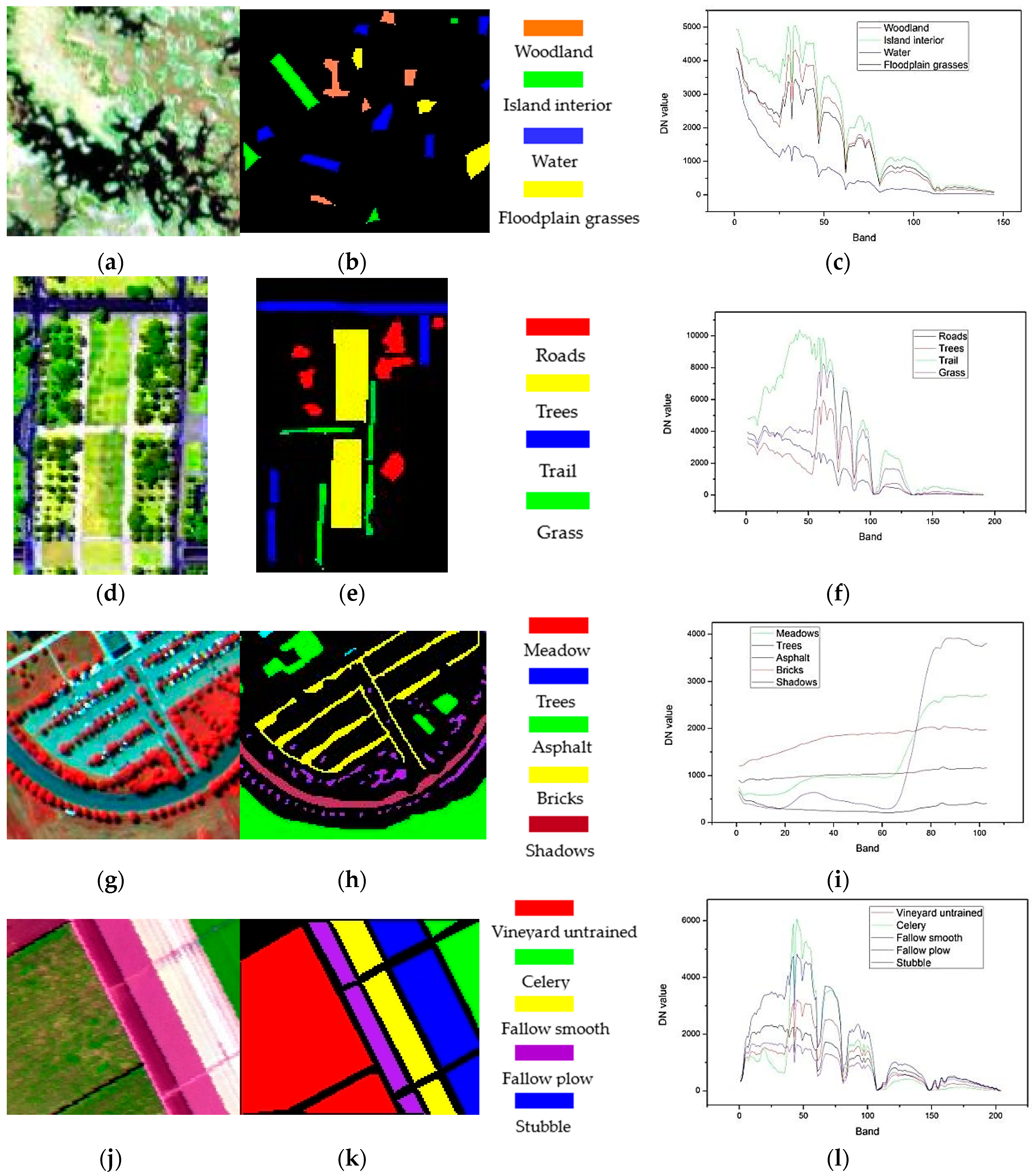
4.1. Datasets
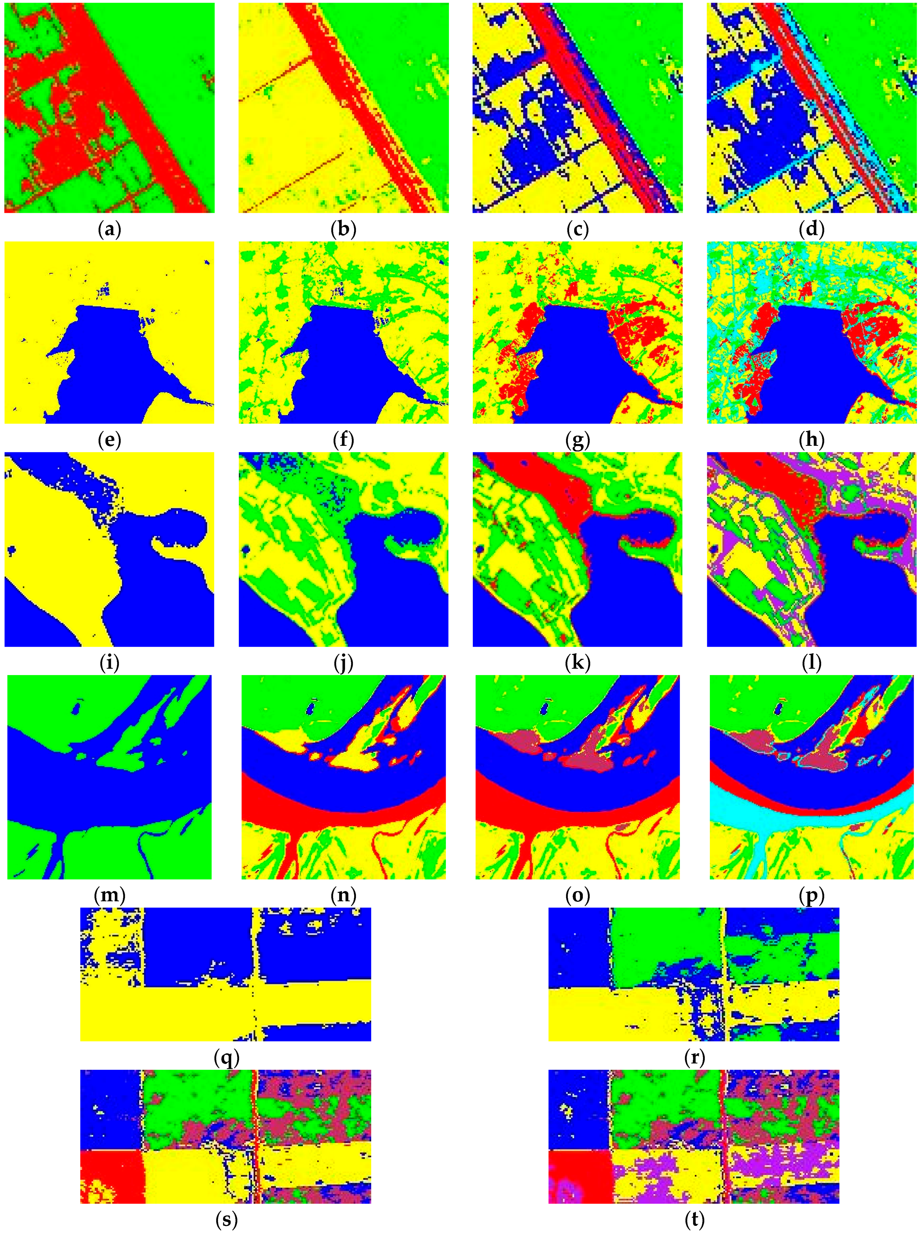
4.2. Results
5. Discussion
6. Conclusions
Acknowledgments
Author Contributions
Conflicts of Interest
References
- Kerr, J.T.; Ostrovsky, M. From space to species: Ecological applications for remote sensing. Trends Ecol. Evol. 2003, 18, 299–305. [Google Scholar] [CrossRef]
- Lu, D.; Weng, Q. A survey of image classification methods and techniques for improving classification performance. Int. J. Remote Sens. 2007, 28, 823–870. [Google Scholar] [CrossRef]
- Otukei, J.R.; Blaschke, T. Land cover change assessment using decision trees, support vector machines and maximum likelihood classification algorithms. Int. J. Appl. Earth Obs. Geoinf. 2010, 12, S27–S31. [Google Scholar] [CrossRef]
- Loveland, T.R.; Reed, B.C.; Brown, J.F.; Ohlen, D.O.; Zhu, Z.; Yang, L.; Merchant, J.W. Development of a global land cover characteristics database and IGBP DISCover from 1 km AVHRR data. Int. J. Remote Sens. 2000, 21, 1303–1330. [Google Scholar] [CrossRef]
- Friedl, M.A.; McIver, D.K.; Hodges, J.C.F.; Zhang, X.Y.; Muchoney, D.; Strahler, A.H.; Woodcock, C.E.; Gopal, S.; Schneider, A.; Cooper, A.; et al. Global land cover mapping from MODIS: Algorithms and early results. Remote Sens. Environ. 2002, 83, 287–302. [Google Scholar] [CrossRef]
- Xiao, X.M.; Boles, S.; Liu, J.Y.; Zhuang, D.F.; Liu, M.L. Characterization of forest types in Northeastern China, using multi-temporal SPOT-4 VEGETATION sensor data. Remote Sens. Environ. 2002, 82, 335–348. [Google Scholar] [CrossRef]
- Schmid, T.; Koch, M.; Gumuzzio, J.; Mather, P.M. A spectral library for a semi-arid wetland and its application to studies of wetland degradation using hyperspectral and multispectral data. Int. J. Remote Sens. 2004, 25, 2485–2496. [Google Scholar] [CrossRef]
- Duda, T.; Canty, M. Unsupervised classification of satellite imagery: Choosing a good algorithm. Int. J. Remote Sens. 2002, 23, 2193–2212. [Google Scholar] [CrossRef]
- Bandyopadhyay, S.; Maulik, U. Genetic clustering for automatic evolution of clusters and application to image classification. Pattern Recognit. 2002, 35, 1197–1208. [Google Scholar] [CrossRef]
- Wang, W.N.; Zhang, Y.J. On fuzzy cluster validity indices. Fuzzy Set Syst. 2007, 158, 2095–2117. [Google Scholar] [CrossRef]
- Halkidi, M.; Batistakis, Y.; Vazirgiannis, M. On clustering validation techniques. J. Intell. Inf. Syst. 2001, 17, 107–145. [Google Scholar] [CrossRef]
- Wu, C.H.; Ouyang, C.S.; Chen, L.W.; Lu, L.W. A new fuzzy clustering validity index with a median factor for centroid-based clustering. IEEE Trans. Fuzzy Syst. 2014, 23, 701–718. [Google Scholar] [CrossRef]
- Sun, H.J.; Wang, S.R.; Jiang, Q.S. FCM-based model selection algorithms for determining the number of clusters. Pattern Recognit. 2004, 37, 2027–2037. [Google Scholar] [CrossRef]
- Das, S.; Abraham, A.; Konar, A. Automatic clustering using an improved differential evolution algorithm. IEEE Trans. Syst Man Cybern. A 2008, 38, 218–237. [Google Scholar] [CrossRef]
- Maulik, U.; Saha, I. Automatic fuzzy clustering using modified differential evolution for image classification. IEEE Trans. Geosci. Remote Sens. 2010, 48, 3503–3510. [Google Scholar] [CrossRef]
- Zhong, Y.F.; Zhang, S.; Zhang, L.P. Automatic fuzzy clustering based on adaptive multi-objective differential evolution for remote sensing imagery. IEEE J. Sel. Top. Appl. Earth Observ. Remote Sens. 2013, 6, 2290–2301. [Google Scholar] [CrossRef]
- Ma, A.L.; Zhong, Y.F.; Zhang, L.P. Adaptive multiobjective memetic fuzzy clustering algorithm for remote sensing imagery. IEEE Trans. Geosci. Remote Sens. 2015, 53, 4202–4217. [Google Scholar] [CrossRef]
- Bandyopadhyay, S.; Pal, S.K. Pixel classification using variable string genetic algorithms with chromosome differentiation. IEEE Trans. Geosci. Remote Sens. 2011, 39, 303–308. [Google Scholar] [CrossRef]
- Rezaee, M.R.; Lelieveldt, B.P.F.; Reiber, J.H.C. A new cluster validity index for the fuzzy c-mean. Pattern Recognit. Lett. 1998, 19, 237–246. [Google Scholar] [CrossRef]
- Pakhira, M.K.; Bandyopadhyay, S.; Maulik, U. A study of some fuzzy cluster validity indices, genetic clustering and application to pixel classification. Fuzzy Sets Syst. 2005, 155, 191–214. [Google Scholar] [CrossRef]
- Arbelaitz, O.; Gurrutxaga, I.; Muguerza, J.; Perez, J.M.; Perona, I. An extensive comparative study of cluster validity indices. Pattern Recognit. 2013, 46, 243–256. [Google Scholar] [CrossRef]
- Bezdek, J.C. Partition Recognition with Fuzzy Objective Function Algorithms; Plenum Press: NewYork, NY, USA, 1981. [Google Scholar]
- Bezdek, J.C. Partition Structures: A Tutorial in the Analysis of Fuzzy Information; CRC Press: Boca Raton, FL, USA, 1987. [Google Scholar]
- Cai, W.L.; Chen, S.C.; Zhang, D.Q. Fast and robust fuzzy c-means clustering algorithms incorporating local information for image segmentation. Pattern Recognit. 2007, 40, 825–838. [Google Scholar] [CrossRef]
- Bezdek, J.C. Cluster validity with fuzzy sets. J. Cybern. 1974, 3, 58–72. [Google Scholar] [CrossRef]
- Dave, R.N. Validating fuzzy partition obtained throughc-shells clustering. Pattern Recognit. Lett. 1996, 17, 613–623. [Google Scholar] [CrossRef]
- Davies, D.L.; Bouldin, D.W. A clustering separation measure. IEEE Trans. Pattern Anal. Mach. Intell. 1979, 1, 224–227. [Google Scholar] [CrossRef] [PubMed]
- Dunn, J.C. A fuzzy relative of the ISODATA process and its use in detecting compact well-separated clusters. J. Cybern. 1973, 3, 32–57. [Google Scholar] [CrossRef]
- Calinski, T.; Harabasz, J. A dendrite method for cluster analysis. Commun Stat. Theory Methods 1974, 3, 1–27. [Google Scholar] [CrossRef]
- Fukuyama, Y.; Sugeno, M. A new method of choosing the number of clusters for fuzzy c-means method. In Proceedings of the 5th Fuzzy System Symposium, Kobe, Japan, 2–3 June 1989.
- Xie, X.L.; Beni, G. A validity measure for fuzzy clustering. IEEE Trans. Pattern Anal. 1991, 13, 841–847. [Google Scholar] [CrossRef]
- Kwon, S.H. Cluster validity index for fuzzy clustering. Electron. Lett. 1998, 34, 2176–2177. [Google Scholar] [CrossRef]
- Tang, Y.G.; Sun, F.C.; Sun, Z.Q. Improved validation index for fuzzy clustering. In Proceedings of the American Control Conference, Portland, OR, USA, 8–10 June 2005.
- Zahid, N.; Limouri, N.; Essaid, A. A new cluster-validity for fuzzy clustering. Pattern Recognit. 1999, 32, 1089–1097. [Google Scholar] [CrossRef]
- Zalik, K.R.; Zalik, B. Validity index for clusters of different sizes and densities. Pattern Recognit. Lett. 2011, 32, 221–234. [Google Scholar] [CrossRef]
- Jain, A.K. Data clustering: 50 years beyond K-means. Pattern Recognit. Lett. 2010, 31, 651–666. [Google Scholar] [CrossRef]
- Wang, L.; Sousa, W.P.; Gong, P.; Biging, G.S. Comparison of IKONOS and QuickBird images for mapping mangrove species on the Caribbean coast of Panama. Remote Sens. Environ. 2004, 91, 432–440. [Google Scholar] [CrossRef]
- Li, J.; Chen, X.L.; Tian, L.Q.; Huang, J.; Feng, L. Improved capabilities of the Chinese high-resolution remote sensing satellite GF-1 for monitoring suspended particulate matter (SPM) in inland waters: Radiometric and spatial considerations. ISPRS J. Photogramm. Remote Sens. 2015, 106, 145–156. [Google Scholar] [CrossRef]
- Tadjudin, S.; Landgrebe, D.A. Robust parameter estimation for mixture model. IEEE Trans. Geosci. Remote Sens. 2000, 38, 439–445. [Google Scholar] [CrossRef]
- Ham, J.; Chen, Y.C.; Crawford, M.M.; Ghosh, J. Investigation of the random forest framework for classification of hyperspectral data. IEEE Trans. Geosci. Remote Sens. 2005, 43, 492–501. [Google Scholar] [CrossRef]
- Yin, J.H.; Wang, Y.F.; Hu, J.K. A new dimensionality reduction algorithm for hyperspectral image using evolutionary strategy. IEEE Trans. Ind. Inform. 2012, 8, 935–943. [Google Scholar] [CrossRef]
- Li, J.; Bioucas-Dias, J.M.; Plaza, A. Spectral-spatial hyperspectral image segmentation using subspace multinomial logistic regression and markov random fields. IEEE Trans. Geosci. Remote Sens. 2012, 50, 809–823. [Google Scholar] [CrossRef]
- Zhou, Y.C.; Peng, J.T.; Chen, C.L.P. Extreme learning machine with composite kernels for hyperspectral image classification. IEEE J. Selected Topics Appl. Earth Observ. Remote Sens. 2015, 8, 2351–2360. [Google Scholar] [CrossRef]
- Kim, D.W.; Lee, K.H.; Lee, D.H. On cluster validity index for estimation of the optimal number of fuzzy clusters. Pattern Recognit. 2004, 37, 2009–2025. [Google Scholar] [CrossRef]
- Maulik, U.; Bandyopadhyay, S. Fuzzy partitioning using a real-coded variable-length genetic algorithm for pixel classification. IEEE Trans. Geosci. Remote Sens. 2003, 41, 1075–1081. [Google Scholar] [CrossRef]
- Paoli, A.; Melgani, F.; Pasolli, E. Clustering of hyperspectral images based on multiobjective particle swarm optimization. IEEE Trans. Geosci. Remote Sens. 2009, 47, 4175–4188. [Google Scholar] [CrossRef]
- Ilc, N. Modified Dunn’s cluster validity index based on graph theory. Electr. Rev. 2012, 2, 126–131. [Google Scholar]
- Pal, N.R.; Bezdek, J.C. Correction to “on cluster validity for the fuzzy c-means model”. IEEE Trans. Fuzzy Syst. 1997, 5, 152–153. [Google Scholar] [CrossRef]


| D | S | Y | L | R | B | W | S | GT |
|---|---|---|---|---|---|---|---|---|
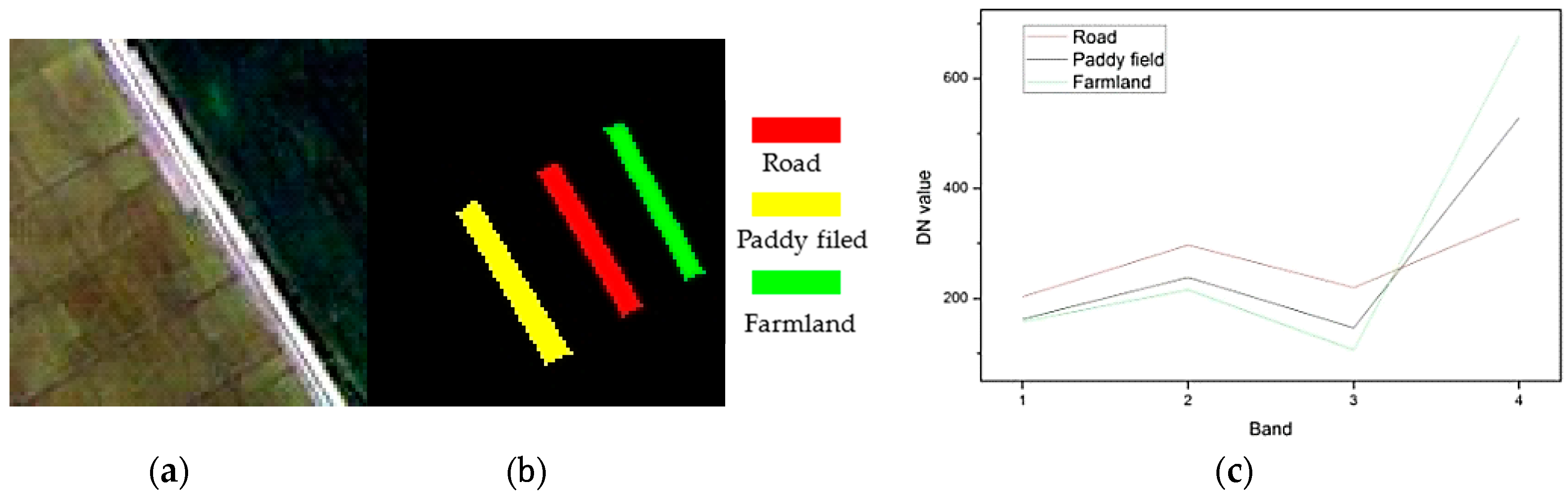
| QuickBird | Multi-spectral camera | 2005 | Yalvhe farm, China | 2.4 | 4 | 0.45–0.90 | 100 × 100 | Road, paddy field, and farmland |
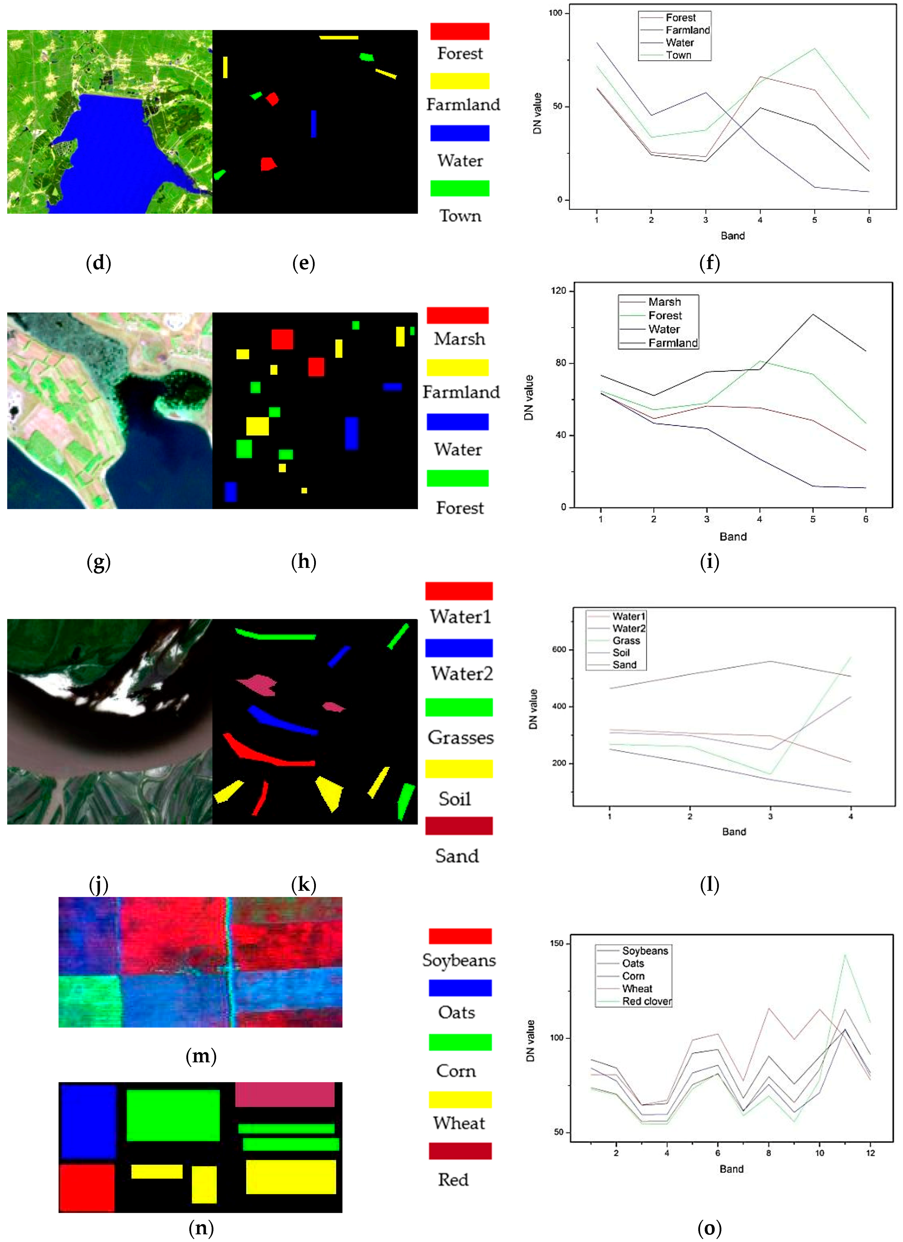
| Landsat TM | Thematic mapper | 2005 | JingYuetan reservoir, China | 30 | 6 | 0.45–2.35 | 296 × 295 | Forest, farmland, water, and town |
| Landsat ETM+ | Enhanced thematic mapper | 2001 | Zhalong reserve, China | 30 | 6 | 0.45–2.35 | 150 × 139 | Marsh, forest, water, and farmland |
| Gaofen-1 | Wide filed imager | 2015 | Sanjiang Plain, China | 16 | 4 | 0.45–0.89 | 200 × 200 | Water1, water2, grass, soil, and sand |
| FLC1 | M7 scanner | 1966 | Tippecanoe County, US | 30 | 12 | 0.40–1.00 | 84 × 183 | Soybeans, oats, corn, wheat and red clover |
| Hyperion | Hyperion | 2001 | Okavango Delta, Botswana | 30 | 145 | 0.40–2.50 | 126 × 146 | Woodland, island interior, water and floodplain grasses |
| HYDICE | HYDICE | 1995 | Washington DC, US | 2 | 191 | 0.40–2.40 | 126 × 82 | Roads, trees, trail and grass |
| ROSIS | ROSIS | 2001 | University of Pavia, Italy | 1.3 | 103 | 0.43–0.86 | 125 × 148 | Meadows, trees, asphalt, bricks and shadows |
| AVIRIS | AVIRIS | 1998 | Salinas Valley, USA | 3.7 | 204 | 0.41–2.45 | 117 × 143 | Vineyard untrained, celery, fallow smooth, fallow plow and stubble |
| Datasets | K# | Overall Accuracies (%) | Kappa Coefficient | ||
|---|---|---|---|---|---|
| FCM | K-Means | FCM | K-Means | ||
| QuickBird | 3 | 96.06 | 96.10 | 0.9354 | 0.9361 |
| Landsat TM | 4 | 95.78 | 95.27 | 0.9433 | 0.9363 |
| Landsat ETM+ | 4 | 94.41 | 96.30 | 0.9253 | 0.9565 |
| Gaofen-1 | 5 | 98.34 | 98.79 | 0.9791 | 0.9848 |
| FLC1 | 5 | 83.10 | 84.48 | 0.7847 | 0.8016 |
| Hyperion | 4 | 87.09 | 86.79 | 0.8260 | 0.8219 |
| HYDICE | 4 | 94.88 | 96.00 | 0.9238 | 0.9403 |
| ROSIS | 5 | 93.85 | 93.25 | 0.9129 | 0.9044 |
| AVIRIS | 5 | 99.63 | 99.63 | 0.9946 | 0.9946 |
| CVIs | Cluster Number | ||||||||
|---|---|---|---|---|---|---|---|---|---|
| 2 | 3 * | 4 | 5 | 6 | 7 | 8 | 9 | 10 | |
| PC+ | 0.754 | 0.800 | 0.728 | 0.699 | 0.658 | 0.623 | 0.626 | 0.593 | 0.579 |
| PE− | 0.565 | 0.532 | 0.749 | 0.866 | 1.008 | 1.134 | 1.150 | 1.272 | 1.341 |
| MPC+ | 0.509 | 0.700 | 0.637 | 0.624 | 0.590 | 0.560 | 0.572 | 0.542 | 0.533 |
| DBI− | 0.822 | 0.559 | 0.692 | 0.750 | 0.779 | 0.845 | 0.802 | 0.882 | 0.915 |
| DI+(e-3) | 2.486 | 3.591 | 2.539 | 2.539 | 2.614 | 2.614 | 3.439 | 3.439 | 3.439 |
| CHI+(e4) | 1.142 | 2.041 | 2.026 | 2.030 | 1.908 | 1.779 | 2.116 | 1.998 | 1.971 |
| FSI−(e7) | −0.535 | −6.644 | −7.247 | −7.331 | −7.093 | −6.902 | −7.440 | −7.260 | −7.092 |
| XBI− | 0.160 | 0.103 | 0.218 | 0.236 | 0.231 | 0.287 | 0.237 | 0.325 | 0.277 |
| KI−(e3) | 1.601 | 1.027 | 2.184 | 2.370 | 2.312 | 2.883 | 2.382 | 3.266 | 2.790 |
| TI−(e3) | 1.601 | 1.029 | 2.189 | 2.376 | 2.320 | 2.894 | 2.395 | 3.284 | 2.808 |
| SCI+ | 0.477 | 2.477 | 2.516 | 2.752 | 2.837 | 2.554 | 3.546 | 3.456 | 3.349 |
| CWBI−(e-2) | 4.076 | 2.826 | 4.284 | 4.964 | 5.399 | 6.902 | 6.592 | 8.628 | 8.499 |
| WSJI− | 0.365 | 0.171 | 0.256 | 0.339 | 0.399 | 0.648 | 0.618 | 1.060 | 1.023 |
| PBMFI+(e3) | 1.588 | 3.214 | 0.635 | 0.336 | 0.068 | 0.060 | 0.022 | 0.034 | 0.013 |
| SVFI+ | 1.422 | 2.415 | 2.621 | 2.910 | 3.063 | 3.252 | 3.517 | 3.699 | 3.885 |
| WLI− | 0.339 | 0.252 | 0.325 | 0.418 | 0.426 | 0.453 | 0.346 | 0.374 | 0.388 |
| CVIs | Cluster Number | ||||||||
|---|---|---|---|---|---|---|---|---|---|
| 2 | 3 | 4 * | 5 | 6 | 7 | 8 | 9 | 10 | |
| PC+ | 0.922 | 0.796 | 0.794 | 0.689 | 0.657 | 0.610 | 0.587 | 0.571 | 0.472 |
| PE− | 0.204 | 0.521 | 0.587 | 0.856 | 0.998 | 1.168 | 1.281 | 1.354 | 1.593 |
| MPC+ | 0.844 | 0.695 | 0.726 | 0.612 | 0.589 | 0.545 | 0.528 | 0.517 | 0.413 |
| DBI− | 0.282 | 0.764 | 0.601 | 0.999 | 0.913 | 1.055 | 1.064 | 1.185 | 1.522 |
| DI+(e-3) | 8.00 | 7.548 | 7.783 | 8.042 | 8.498 | 8.893 | 8.893 | 8.893 | 8.893 |
| CHI+(e5) | 2.883 | 2.608 | 3.261 | 2.914 | 2.831 | 2.568 | 2.393 | 2.348 | 2.053 |
| FSI−(e7) | −6.762 | −7.850 | −8.743 | −8.423 | −8.342 | −8.132 | −8.027 | −7.945 | −5.888 |
| XBI− | 0.044 | 0.177 | 0.092 | 0.599 | 0.450 | 0.626 | 0.564 | 0.661 | 2.025 |
| KI−(e4) | 0.334 | 1.335 | 0.693 | 4.523 | 3.402 | 4.731 | 4.259 | 4.996 | 15.300 |
| TI−(e4) | 0.334 | 1.335 | 0.693 | 4.515 | 3.397 | 4.721 | 4.251 | 4.985 | 15.188 |
| SCI+ | 3.463 | 3.319 | 3.876 | 3.609 | 3.407 | 2.916 | 3.204 | 2.362 | 3.439 |
| CWBI−(e-2) | 0.151 | 0.142 | 0.114 | 0.291 | 0.299 | 0.403 | 0.425 | 0.457 | 0.762 |
| WSJI− | 0.167 | 0.094 | 0.057 | 0.154 | 0.159 | 0.274 | 0.307 | 0.372 | 1.015 |
| PBMFI+(e3) | 1.014 | 0.296 | 0.018 | 0.013 | 0.006 | 0.006 | 0.001 | 0.001 | 0.001 |
| SVFI+ | 1.922 | 2.287 | 2.982 | 3.367 | 3.816 | 4.106 | 4.349 | 4.224 | 3.137 |
| WLI− | 0.079 | 0.131 | 0.172 | 0.247 | 0.327 | 0.361 | 0.463 | 0.395 | 0.293 |
| CVIs | Cluster Number | ||||||||
|---|---|---|---|---|---|---|---|---|---|
| 2 | 3 | 4 * | 5 | 6 | 7 | 8 | 9 | 10 | |
| PC+ | 0.404 | 0.812 | 0.760 | 0.725 | 0.703 | 0.663 | 0.628 | 0.617 | 0.593 |
| PE− | 0.284 | 0.503 | 0.673 | 0.802 | 0.877 | 1.012 | 1.144 | 1.204 | 1.300 |
| MPC+ | 0.775 | 0.717 | 0.680 | 0.656 | 0.644 | 0.607 | 0.575 | 0.569 | 0.548 |
| DBI− | 0.404 | 0.603 | 0.674 | 0.731 | 0.745 | 0.861 | 0.952 | 0.937 | 1.055 |
| DI+(e-3) | 5.803 | 7.595 | 8.256 | 8.889 | 8.889 | 0.104 | 0.107 | 0.107 | 0.114 |
| CHI+(e5) | 0.818 | 0.909 | 0.929 | 0.929 | 0.896 | 0.893 | 0.847 | 0.847 | 0.822 |
| FSI−(e8) | −0.409 | −0.483 | −0.477 | −0.461 | −0.461 | −0.439 | −0.426 | −0.422 | −0.413 |
| XBI− | 0.047 | 0.090 | 0.117 | 0.169 | 0.183 | 0.202 | 0.234 | 0.216 | 0.293 |
| KI−(e4) | 0.100 | 0.188 | 0.244 | 0.352 | 0.382 | 0.421 | 0.489 | 0.452 | 0.613 |
| TI−(e4) | 0.099 | 0.189 | 0.244 | 0.353 | 0.383 | 0.422 | 0.490 | 0.454 | 0.615 |
| SCI+ | 2.463 | 3.259 | 3.388 | 3.723 | 4.715 | 5.137 | 4.922 | 4.779 | 4.884 |
| CWBI− | 0.054 | 0.059 | 0.076 | 0.104 | 0.112 | 0.133 | 0.164 | 0.174 | 0.226 |
| WSJI− | 0.162 | 0.351 | 0.126 | 0.214 | 0.248 | 0.348 | 0.515 | 0.601 | 1.012 |
| PBMFI+(e3) | 1.058 | 0.156 | 0.085 | 0.088 | 0.004 | 0.005 | 0.002 | 0.014 | 0.003 |
| SVFI+ | 2.173 | 2.413 | 3.027 | 0.760 | 3.155 | 3.339 | 3.521 | 3.607 | 3.648 |
| WLI− | 0.093 | 0.174 | 0.307 | 0.265 | 0.244 | 0.229 | 0.259 | 0.208 | 0.279 |
| CVIs | Cluster Number | ||||||||
|---|---|---|---|---|---|---|---|---|---|
| 2 | 3 | 4 | 5 * | 6 | 7 | 8 | 9 | 10 | |
| PC+ | 0.850 | 0.751 | 0.764 | 0.779 | 0.735 | 0.710 | 0.688 | 0.669 | 0.645 |
| PE− | 0.374 | 0.643 | 0.663 | 0.658 | 1.183 | 0.900 | 0.978 | 1.056 | 1.140 |
| MPC+ | 0.700 | 0.627 | 0.620 | 0.724 | 0.682 | 0.662 | 0.643 | 0.628 | 0.606 |
| DBI− | 0.587 | 0.832 | 0.767 | 0.536 | 0.701 | 0.740 | 0.789 | 0.803 | 0.896 |
| DI+(e-3) | 4.715 | 1.478 | 1.470 | 2.298 | 2.348 | 2.688 | 3.028 | 2.860 | 2.965 |
| CHI+(e5) | 0.764 | 0.656 | 0.681 | 1.314 | 1.185 | 1.262 | 1.270 | 1.257 | 1.197 |
| FSI−(e9) | −0.662 | −1.038 | −1.253 | −1.603 | −1.571 | −1.539 | −1.519 | −1.490 | −1.462 |
| XBI− | 0.100 | 0.135 | 0.136 | 0.077 | 0.198 | 0.158 | 0.140 | 0.154 | 0.285 |
| KI−(e4) | 0.399 | 0.541 | 0.546 | 0.309 | 0.791 | 0.634 | 0.560 | 0.617 | 1.141 |
| TI−(e4) | 0.399 | 0.541 | 0.546 | 0.309 | 0.792 | 0.635 | 0.561 | 0.618 | 1.141 |
| SCI+ | 1.031 | 1.156 | 1.364 | 4.658 | 3.899 | 4.468 | 4.470 | 4.333 | 3.992 |
| CWBI−(e-3) | 0.147 | 0.137 | 0.144 | 0.139 | 0.240 | 0.264 | 0.268 | 0.311 | 0.445 |
| WSJI− | 0.226 | 0.934 | 0.128 | 0.114 | 0.282 | 0.348 | 0.362 | 0.487 | 1.015 |
| PBMFI+(e4) | 1.049 | 0.243 | 0.075 | 0.053 | 0.063 | 0.019 | 0.011 | 0.040 | 0.056 |
| SVFI+ | 2.315 | 2.610 | 3.027 | 3.707 | 3.739 | 4.193 | 4.009 | 4.245 | 4.165 |
| WLI− | 0.201 | 0.342 | 0.307 | 0.154 | 0.174 | 0.202 | 0.196 | 0.208 | 0.226 |
| CVIs | Cluster Number | ||||||||
|---|---|---|---|---|---|---|---|---|---|
| 2 | 3 | 4 | 5 * | 6 | 7 | 8 | 9 | 10 | |
| PC+ | 0.760 | 0.680 | 0.584 | 0.602 | 0.555 | 0.497 | 0.451 | 0.429 | 0.398 |
| PE− | 0.549 | 0.834 | 1.139 | 1.160 | 1.343 | 1.556 | 1.724 | 1.831 | 1.974 |
| MPC+ | 0.519 | 0.520 | 0.446 | 0.503 | 0.466 | 0.414 | 0.372 | 0.358 | 0.331 |
| DBI− | 0.887 | 0.909 | 1.052 | 0.896 | 0.937 | 1.008 | 1.432 | 1.410 | 1.475 |
| DI+(e-2) | 0.806 | 1.330 | 1.048 | 1.613 | 1.365 | 1.495 | 1.259 | 1.259 | 1.542 |
| CHI+(e4) | 1.274 | 1.537 | 1.273 | 1.616 | 1.521 | 1.354 | 1.249 | 1.194 | 1.105 |
| FSI−(e6) | −0.666 | −5.029 | −5.479 | −8.809 | −8.573 | −7.979 | −7.511 | −7.200 | −6.794 |
| XBI− | 0.206 | 0.186 | 0.380 | 0.224 | 0.268 | 0.334 | 0.636 | 0.616 | 0.576 |
| KI−(e4) | 0.299 | 0.270 | 0.552 | 0.325 | 0.390 | 0.485 | 0.924 | 0.896 | 0.837 |
| TI−(e4) | 0.299 | 0.270 | 0.552 | 0.325 | 0.390 | 0.485 | 0.924 | 0.896 | 0.838 |
| SCI+ | 0.307 | 0.624 | 0.383 | 0.913 | 1.089 | 0.672 | 0.639 | 0.815 | 0.681 |
| CWBI− | 0.126 | 0.098 | 0.123 | 0.109 | 0.128 | 0.154 | 0.221 | 0.230 | 0.238 |
| WSJI− | 0.410 | 0.598 | 0.294 | 0.241 | 0.305 | 0.425 | 0.877 | 0.968 | 1.049 |
| PBMFI+ | 186.178 | 84.915 | 27.891 | 5.076 | 16.638 | 5.969 | 5.374 | 2.140 | 0.932 |
| SVFI+ | 1.185 | 1.874 | 2.389 | 3.040 | 3.424 | 3.680 | 3.439 | 3.679 | 3.803 |
| WLI− | 0.415 | 0.535 | 0.708 | 0.523 | 0.584 | 0.709 | 7.591 | 0.727 | 0.777 |
| CVIs | Cluster Number | ||||||||
|---|---|---|---|---|---|---|---|---|---|
| 2 | 3 | 4 * | 5 | 6 | 7 | 8 | 9 | 10 | |
| PC+ | 0.867 | 0.759 | 0.682 | 0.658 | 0.596 | 0.568 | 0.530 | 0.494 | 0.476 |
| PE− | 0.337 | 0.626 | 0.869 | 0.973 | 1.176 | 1.293 | 1.435 | 1.577 | 1.666 |
| MPC+ | 0.735 | 0.638 | 0.576 | 0.573 | 0.515 | 0.496 | 0.463 | 0.430 | 0.417 |
| DBI− | 0.472 | 0.651 | 0.732 | 0.726 | 0.853 | 0.856 | 0.946 | 1.060 | 1.032 |
| DI+(e-2) | 2.169 | 2.979 | 2.837 | 2.900 | 3.489 | 3.332 | 3.518 | 2.971 | 3.916 |
| CHI+(e4) | 4.690 | 5.329 | 5.328 | 5.779 | 5.485 | 5.383 | 5.158 | 4.925 | 4.846 |
| FSI−(e11) | −4.610 | −6.600 | −6.902 | −7.003 | −6.808 | −6.619 | −6.414 | −6.209 | −6.039 |
| XBI− | 0.061 | 0.139 | 0.157 | 0.149 | 0.217 | 0.193 | 0.228 | 0.275 | 0.239 |
| KI−(e3) | 1.131 | 2.552 | 2.888 | 2.750 | 3.995 | 3.560 | 4.201 | 5.064 | 4.400 |
| TI−(e3) | 1.131 | 2.555 | 2.892 | 2.755 | 4.004 | 3.569 | 4.213 | 5.080 | 4.416 |
| SCI+ | 2.241 | 3.109 | 3.161 | 4.201 | 4.012 | 4.586 | 4.574 | 4.469 | 4.605 |
| CWBI−(e-3) | 0.440 | 0.485 | 0.597 | 0.651 | 0.900 | 0.929 | 1.118 | 1.347 | 1.333 |
| WSJI− | 0.244 | 0.681 | 0.207 | 0.244 | 0.446 | 0.491 | 0.706 | 1.019 | 1.020 |
| PBMFI+(e6) | 4.131 | 6.247 | 1.732 | 0.319 | 0.528 | 0.325 | 0.184 | 0.009 | 0.005 |
| SVFI+ | 2.204 | 2.459 | 2.867 | 3.124 | 3.307 | 3.536 | 3.697 | 3.764 | 3.885 |
| WLI− | 1.222 | 0.185 | 0.241 | 0.231 | 0.242 | 0.244 | 0.254 | 0.281 | 0.307 |
| CVIs | Cluster Number | ||||||||
|---|---|---|---|---|---|---|---|---|---|
| 2 | 3 | 4 * | 5 | 6 | 7 | 8 | 9 | 10 | |
| PC+ | 0.752 | 0.729 | 0.669 | 0.621 | 0.587 | 0.554 | 0.541 | 0.511 | 0.502 |
| PE− | 0.573 | 0.717 | 0.922 | 1.106 | 1.246 | 1.382 | 1.471 | 1.598 | 1.656 |
| MPC+ | 0.504 | 0.594 | 0.558 | 0.526 | 0.505 | 0.479 | 0.475 | 0.450 | 0.447 |
| DBI− | 0.888 | 0.669 | 0.747 | 0.824 | 0.828 | 0.899 | 0.827 | 0.888 | 0.888 |
| DI+(e-2) | 1.194 | 1.070 | 1.165 | 1.236 | 1.081 | 1.190 | 1.897 | 1.098 | 1.089 |
| CHI+(e4) | 1.057 | 1.494 | 1.473 | 1.618 | 1.606 | 1.508 | 1.634 | 1.587 | 1.594 |
| FSI−(e12) | 0.004 | −1.258 | −1.511 | −1.592 | −1.627 | −1.603 | −1.608 | −1.579 | −1.567 |
| XBI− | 0.196 | 0.105 | 0.149 | 0.168 | 0.231 | 0.258 | 0.223 | 0.315 | 0.260 |
| KI−(e3) | 2.025 | 1.084 | 1.545 | 1.733 | 2.393 | 2.671 | 2.306 | 3.258 | 2.694 |
| TI−(e3) | 2.026 | 1.085 | 1.547 | 1.737 | 2.398 | 2.678 | 2.313 | 3.268 | 2.704 |
| SCI+ | 0.391 | 1.878 | 1.906 | 1.997 | 2.151 | 1.733 | 1.911 | 1.691 | 1.901 |
| CWBI−(e-4) | 2.538 | 1.761 | 2.017 | 2.395 | 3.082 | 3.508 | 3.585 | 4.598 | 4.398 |
| WSJI− | 0.422 | 1.082 | 0.229 | 0.299 | 0.482 | 0.621 | 0.671 | 1.111 | 1.034 |
| PBMFI+(e6) | 27.978 | 28.242 | 7.311 | 1.490 | 2.274 | 1.228 | 0.250 | 0.655 | 0.118 |
| SVFI+ | 1.560 | 2.490 | 2.928 | 3.298 | 3.566 | 3.689 | 4.202 | 4.352 | 4.349 |
| WLI− | 0.390 | 0.263 | 0.288 | 0.323 | 0.388 | 0.406 | 0.475 | 0.474 | 0.387 |
| CVIs | Cluster Number | ||||||||
|---|---|---|---|---|---|---|---|---|---|
| 2 | 3 | 4 | 5 * | 6 | 7 | 8 | 9 | 10 | |
| PC+ | 0.703 | 0.664 | 0.615 | 0.594 | 0.548 | 0.504 | 0.477 | 0.461 | 0.443 |
| PE− | 0.661 | 0.878 | 1.076 | 1.204 | 1.381 | 1.541 | 1.672 | 1.775 | 1.874 |
| MPC+ | 0.406 | 0.495 | 0.486 | 0.492 | 0.457 | 0.421 | 0.403 | 0.393 | 0.381 |
| DBI− | 1.305 | 0.796 | 0.894 | 0.876 | 1.001 | 1.464 | 1.405 | 1.371 | 1.349 |
| DI+(e-2) | 0.580 | 0.656 | 0.711 | 0.678 | 0.676 | 0.606 | 0.628 | 0.562 | 0.562 |
| CHI+(e4) | 0.834 | 1.323 | 1.217 | 1.109 | 1.000 | 0.980 | 0.905 | 0.844 | 0.777 |
| FSI−(e11) | 2.514 | −1.127 | −1.939 | −2.526 | −2.678 | −2.627 | −2.636 | −2.671 | −2.637 |
| XBI− | 0.427 | 0.158 | 0.273 | 0.213 | 0.481 | 0.715 | 0.666 | 0.623 | 0.591 |
| KI−(e4) | 0.790 | 0.293 | 0.506 | 0.394 | 0.890 | 1.324 | 1.233 | 1.154 | 1.094 |
| TI−(e4) | 0.790 | 0.293 | 0.506 | 0.394 | 0.891 | 1.325 | 1.234 | 1.155 | 1.095 |
| SCI+ | −0.011 | 0.316 | 0.287 | 0.390 | 0.206 | 0.333 | 0.179 | 0.147 | 0.591 |
| CWBI−(e-3) | 0.731 | 0.424 | 0.493 | 0.451 | 0.700 | 0.872 | 0.946 | 1.009 | 1.082 |
| WSJI− | 0.502 | 0.743 | 0.261 | 0.224 | 0.432 | 0.660 | 0.789 | 0.913 | 1.058 |
| PBMFI+(e6) | 2.883 | 1.809 | 0.068 | 0.014 | 0.010 | 0.015 | 0.007 | 0.003 | 0.002 |
| SVFI+ | 0.569 | 1.720 | 2.187 | 2.958 | 3.290 | 3.163 | 3.658 | 4.011 | 4.288 |
| WLI− | 0.859 | 0.453 | 0.624 | 0.665 | 0.872 | 0.678 | 0.848 | 0.857 | 0.848 |
| CVIs | Cluster Number | ||||||||
|---|---|---|---|---|---|---|---|---|---|
| 2 | 3 | 4 | 5 * | 6 | 7 | 8 | 9 | 10 | |
| PC+ | 0.843 | 0.838 | 0.856 | 0.732 | 0.763 | 0.700 | 0.681 | 0.661 | 0.631 |
| PE− | 0.395 | 0.451 | 0.451 | 0.760 | 0.691 | 0.889 | 0.945 | 1.014 | 1.135 |
| MPC+ | 0.686 | 0.757 | 0.808 | 0.665 | 0.715 | 0.650 | 0.636 | 0.619 | 0.590 |
| DBI− | 0.690 | 0.557 | 0.383 | 0.689 | 0.617 | 0.802 | 0.864 | 0.949 | 0.962 |
| DI+(e-2) | 0.615 | 1.524 | 1.567 | 0.871 | 1.198 | 1.236 | 1.523 | 1.297 | 1.312 |
| CHI+(e4) | 2.105 | 2.991 | 5.686 | 4.681 | 6.460 | 5.642 | 6.716 | 6.230 | 5.556 |
| FSI−(e11) | −1.098 | −4.465 | −6.317 | −5.999 | −6.803 | −6.631 | −6.331 | −6.151 | −6.004 |
| XBI− | 0.117 | 0.125 | 0.065 | 0.797 | 0.562 | 0.948 | 0.696 | 0.643 | 0.829 |
| KI−(e4) | 0.195 | 0.210 | 0.109 | 1.335 | 0.943 | 1.589 | 1.168 | 1.080 | 1.394 |
| TI−(e4) | 0.195 | 0.210 | 0.109 | 1.338 | 0.946 | 1.595 | 1.173 | 1.086 | 1.401 |
| SCI+ | 1.113 | 1.958 | 4.715 | 3.844 | 5.684 | 4.813 | 5.351 | 5.869 | 6.006 |
| CWBI−(e-3) | 0.982 | 0.545 | 0.407 | 1.257 | 1.367 | 2.082 | 1.938 | 1.997 | 2.376 |
| WSJI− | 0.360 | 0.665 | 0.079 | 0.276 | 0.335 | 0.742 | 0.676 | 0.721 | 1.016 |
| PBMFI+(e5) | 21.751 | 14.564 | 0.855 | 4.139 | 0.950 | 1.279 | 1.925 | 0.910 | 1.002 |
| SVFI+ | 1.942 | 2.653 | 3.414 | 3.544 | 3.620 | 4.129 | 3.422 | 3.220 | 3.007 |
| WLI− | 0.235 | 0.213 | 0.127 | 0.173 | 0.149 | 0.200 | 0.158 | 0.152 | 0.135 |
| Images | K# | PC | PE | MPC | DBI | DI | CHI | FSI | SCI |
| Multispectral image | |||||||||
| QuickBird | 3 | 3 * | 3 * | 3 * | 3 * | 3 * | 8 | 8 | 8 |
| Landsat TM | 4 | 2 | 2 | 2 | 2 | 7 | 4 * | 4 * | 4 * |
| Landsat ETM+ | 4 | 3 | 2 | 2 | 2 | 5 | 4 * | 3 | 7 |
| GaoFen-1 | 5 | 2 | 2 | 5 * | 5 * | 2 | 5 * | 5 * | 5 * |
| FLC1 | 5 | 2 | 2 | 3 | 2 | 5 * | 5 * | 5 * | 6 |
| Hyperspectral image | |||||||||
| Hyperion | 4 | 2 | 2 | 2 | 2 | 10 | 5 | 6 | 10 |
| HYDICE | 4 | 2 | 2 | 3 | 3 | 8 | 5 | 6 | 6 |
| ROSIS | 5 | 4 | 2 | 4 | 4 | 4 | 8 | 6 | 10 |
| AVIRIS | 5 | 2 | 2 | 3 | 3 | 4 | 3 | 6 | 10 |
| Images | C | XBI | KI | TI | CWBI | WSJI | PBMFI | SVFI | WLI |
| Multispectral image | |||||||||
| QuickBird | 3 | 3 * | 3 * | 3 * | 3 * | 3 * | 3 * | 10 | 3 * |
| Landsat TM | 4 | 2 | 2 | 2 | 4 * | 4 * | 2 | 8 | 2 |
| Landsat ETM+ | 4 | 2 | 2 | 2 | 2 | 4 * | 2 | 10 | 2 |
| GaoFen-1 | 5 | 5 * | 5 * | 5 * | 3 | 5 * | 2 | 7 | 5 * |
| FLC1 | 5 | 3 | 3 | 3 | 3 | 5 * | 2 | 10 | 2 |
| Hyperspectral image | |||||||||
| Hyperion | 4 | 2 | 2 | 2 | 2 | 4 * | 3 | 10 | 3 |
| HYDICE | 4 | 3 | 3 | 3 | 3 | 4 * | 3 | 9 | 3 |
| ROSIS | 5 | 3 | 3 | 3 | 3 | 5 * | 2 | 10 | 3 |
| AVIRIS | 5 | 4 | 4 | 4 | 4 | 4 | 2 | 7 | 4 |
| Images | K# | PC | PE | MPC | DBI | DI | CHI | FSI | SCI |
| Multispectral image | |||||||||
| QuickBird | 3 | 2 | 2 | 3 * | 3 * | 3 * | 9 | 7 | 7 |
| Landsat TM | 4 | 2 | 2 | 2 | 2 | 8 | 4 * | 4 * | 4 * |
| Landsat ETM+ | 4 | 2 | 2 | 2 | 2 | 9 | 4 * | 4 * | 9 |
| GaoFen-1 | 5 | 2 | 2 | 5 * | 5 * | 2 | 5 * | 5 * | 5 * |
| Hyperspectral image | |||||||||
| Hyperion | 4 | 2 | 2 | 2 | 2 | 7 | 5 | 5 | 7 |
| HYDICE | 4 | 2 | 2 | 3 | 3 | 7 | 7 | 7 | 5 |
| ROSIS | 5 | 2 | 2 | 3 | 3 | 4 | 3 | 9 | 9 |
| AVIRIS | 5 | 2 | 2 | 3 | 3 | 4 | 3 | 6 | 10 |
| Images | C | XBI | KI | TI | CWBI | WSJI | PBMFI | SVFI | WLI |
| Multispectral image | |||||||||
| QuickBird | 3 | 3 * | 3 * | 3 * | 3 * | 3 * | 3 * | 10 | 2 |
| Landsat TM | 4 | 2 | 2 | 2 | 2 | 4 * | 2 | 10 | 2 |
| Landsat ETM+ | 4 | 2 | 2 | 2 | 3 | 4 * | 2 | 10 | 2 |
| GaoFen-1 | 5 | 5 * | 5 * | 5 * | 5 * | 5 * | 2 | 9 | 5 * |
| Hyperspectral image | |||||||||
| Hyperion | 4 | 2 | 2 | 2 | 2 | 4 * | 3 | 10 | 2 |
| HYDICE | 4 | 5 | 5 | 5 | 3 | 4 * | 2 | 10 | 3 |
| ROSIS | 5 | 6 | 6 | 6 | 3 | 5 * | 2 | 10 | 3 |
| AVIRIS | 5 | 4 | 4 | 4 | 4 | 4 | 2 | 7 | 4 |
© 2016 by the authors; licensee MDPI, Basel, Switzerland. This article is an open access article distributed under the terms and conditions of the Creative Commons by Attribution (CC-BY) license (http://creativecommons.org/licenses/by/4.0/).
Share and Cite
Li, H.; Zhang, S.; Ding, X.; Zhang, C.; Dale, P. Performance Evaluation of Cluster Validity Indices (CVIs) on Multi/Hyperspectral Remote Sensing Datasets. Remote Sens. 2016, 8, 295. https://doi.org/10.3390/rs8040295
Li H, Zhang S, Ding X, Zhang C, Dale P. Performance Evaluation of Cluster Validity Indices (CVIs) on Multi/Hyperspectral Remote Sensing Datasets. Remote Sensing. 2016; 8(4):295. https://doi.org/10.3390/rs8040295
Chicago/Turabian StyleLi, Huapeng, Shuqing Zhang, Xiaohui Ding, Ce Zhang, and Patricia Dale. 2016. "Performance Evaluation of Cluster Validity Indices (CVIs) on Multi/Hyperspectral Remote Sensing Datasets" Remote Sensing 8, no. 4: 295. https://doi.org/10.3390/rs8040295