Article

A New Soil Moisture Agricultural Drought Index (SMADI) Integrating MODIS and SMOS Products: A Case of Study over the Iberian Peninsula

by
Nilda Sánchez
1,*,
Ángel González-Zamora
1,
María Piles
2 and
José Martínez-Fernández
1
1
Instituto Hispano Luso de Investigaciones Agrarias, University of Salamanca, Duero 12, 37185 Villamayor (Salamanca), Spain
2
Barcelona Expert Center, Institute of Marine Sciences, CSIC, Passeig Marítim de la Barceloneta, 37-49, 08003 Barcelona, Spain
*
Author to whom correspondence should be addressed.
Remote Sens. 2016, 8(4), 287; https://doi.org/10.3390/rs8040287
Submission received: 10 February 2016 / Revised: 14 March 2016 / Accepted: 22 March 2016 / Published: 29 March 2016

Abstract

:
A new index for agricultural drought monitoring is presented based on the integration of different soil/vegetation remote sensing observations. The synergistic fusion of the surface soil moisture (SSM) from the Soil Moisture and Ocean Salinity (SMOS) mission, with the Moderate Resolution Imaging Spectroradiometer (MODIS) derived land surface temperature (LST), and water/vegetation indices for agricultural drought monitoring was tested. The rationale of the approach is based on the inverse relationship between LST, vegetation condition and soil moisture content. Thus, the proposed Soil Moisture Agricultural Drought Index (SMADI) combines the soil and temperature conditions while including the lagged response of vegetation. SMADI was retrieved every eight days at 500 m spatial resolution for the whole Iberian Peninsula (IP) from 2010 to 2014, and a time lag of eight days was used to account for the plant response to the varying soil/climatic conditions. The results of SMADI compared well with other agricultural indices in a semiarid area in the Duero basin, in Spain, and also with a climatic index in areas of the Iberian Peninsula under contrasted climatic conditions. Based on a standard classification of drought severity, the proposed index allowed for a coherent description of the drought conditions of the IP during the study period.

Graphical Abstract

1. Introduction

Most drought definitions [1,2,3,4] rely on its area of impact. Broadly, an agricultural drought refers to soil water deficit, whereas a meteorological drought is characterized by a prolonged and abnormal deficiency of precipitation. Streamflow/groundwater deficit is applied if hydrological drought is considered, which in turn implies a long, persistent meteorological drought. Besides, socioeconomic drought is related to the surplus of demand of economic goods as a result of a weather-related shortfall in water supply that affects population. Another emerging definition that is gaining widespread use in recent years is flash drought, defined as a severe, short-term event characterized by soil moisture deficit and abnormally high temperatures, thus negatively impacting vegetation conditions [5,6].
Drought indices are used for identifying, classifying and monitoring drought conditions. They allow quantitative assessment of intensity, duration and spatial extent of anomalous climatic conditions and therefore support decision-making systems (e.g., triggering mitigation actions). Traditional drought indices are either precipitation-based only, such as the Standardized Precipitation Index, SPI [7] or based in water demand (evapotranspiration) and losses (runoff), such as the Palmer Drought Severity Index, PDSI [8]. Both indices are long-term drought estimators but not drought prediction tools. In shorter time scales, the Crop Moisture Index [9] aims at assessing the agricultural drought. The agriculture production is closely linked to actual crop evapotranspiration, which is in turn usually monitored by the water balance of the whole crop growing cycle [10]. According to moisture conditions and deficiency or surplus of water for a given area, drought indices can be classified as precipitation indices, water balance indices, soil moisture indices and aridity indices [3]. It is appropriate to point out that, in most cases, not a single indicator, but several at once, are used to get a full characterization of drought in a given area. Also, as the characterization of the drought condition is based on discrete measurements (mainly at scattered weather stations), the spatial distribution and extent of drought events at the regional scale is challenging. In this regard, the use of remotely sensed information may help providing spatially distributed information. In particular, a drought index based in soil moisture content, vegetation status and surface temperature (considering short-term estimations of all of them) would include the main factors describing drought effects and causes, and would be suitable for agricultural drought monitoring in a medium-short term. Due to its linking-processes condition, soil moisture is placed squarely in the center of the spectrum of drought classifications and drought indicators [11]. The information of soil moisture is key in drought monitoring, as the soil water content can drastically be depleted when there is a precipitation deficit. Hence, soil moisture provides direct evidence of areas suffering rain shortage. There are currently a variety of reliable and feasible methods to measure soil water content from the point scale to the global scale [12]. Among them, soil moisture satellite products offer considerable advantages in terms of global coverage, temporal and spatial resolution, and are recently being integrated in drought monitoring programs [10]. Currently, there are two missions devoted to global surface soil moisture (SSM, top 0–5 cm) monitoring: the Soil Moisture and Ocean Salinity (SMOS) [13] and the Soil Moisture Active and Passive (SMAP) [14]. These two missions provide 40 km global maps of SSM every three days. New end-level L4 products for drought monitoring based on SMOS and SMAP data are being developed, either from model assimilation or fusion with other remotely sensed data [15]. Although the agricultural drought is typically defined in the root zone (about 1 m depth), information of SSM is valuable to link the soil water content on the surface to the root depth and reduce the uncertainties associated with other processes of drought estimation. Also, several strategies of disaggregation or fusion of SMOS/SMAP have been developed to provide soil moisture information at scales finer than 40 km. Among them, the well-known relationship between radiative temperature and vegetation state with surface soil water content [16] has been shown to be a feasible basis to enhance the spatial resolution of microwave-derived soil moisture information from spaceborne and airborne observations [17,18,19]. Besides the spatial resolution improvement of the SSM product, the addition of the vegetation proxy would help to overcome the mismatch between the SMOS depth observations and the actual root zone depth, where the water deficit is actually influencing the vegetation developing. Also, because of a lagged vegetation response to rainfall deficits due to residual moisture stored in the soil, indices such as the Normalized Difference Vegetation Index (NDVI) have a lagged response to drought [20,21,22,23,24], thus NDVI may not be a good index for monitoring drought without concerning the time lag [10].
Many of the drought monitoring approaches with satellite remotely sensed data are usually based on NDVI, land surface temperature (LST) (alternatively brightness temperature), or a combination of them. The so-called vegetative drought indices, mainly based on the NDVI (e.g., NDVI anomaly, integrated or standardized NDVI, Vegetation Condition Index, etc.) have been widely and successfully used to identify and monitor areas affected by drought at regional and local scales [25,26,27,28,29]. The NDVI for each pixel normalized with the maximum and minimum statistical range over the available imagery was proposed by Kogan [30] to develop the Vegetation Condition Index (VCI) as an indicator of environmental stress [31]. Following the VCI definition, the available moisture determines the NDVI minimum while the historical maximum is determined by weather conditions. Thus, the NDVI acts as a synoptic indicator between the soil and the atmospheric conditions while describing the plant status.
The World Agricultural Outlook Board from the United States Department of Agriculture, as well as the National Drought Mitigation Center of the U.S. suggests that an integrated drought monitoring system needs to couple climate, soil and water data, incorporating local and regional scale data and using multiple indices and triggering tools for early warning systems [32]. Agricultural drought does not begin with the rain decrease, but rather when available stored water supports actual evapotranspiration at only a small fraction of the potential evapotranspiration rate [33]. In this regard, an agricultural drought index should integrate various parameters like rainfall, temperature, evapotranspiration, runoff, and other water supply indicators that impact crop growth and development during drought episodes into a single number [34]. For example, in a drought situation, the soil water scarcity is often aggravated by an increased heat load due to less cloudiness. Thus, indicators of soil moisture, temperature and plant status seem to provide a comprehensive suite for predicting agricultural drought.
In this work, a synergistic integration of SMOS-SSM with MODIS-derived LST and water/vegetation indices for agricultural drought monitoring was explored. A new drought index, hereafter the Soil Moisture Agricultural Drought Index (SMADI), including actual soil and temperature conditions, with lagged information on vegetation, is proposed to detect and characterize soil moisture drought conditions with particular emphasis on short-term agricultural droughts, which are key to crop success. We hypothesize that the well-known synergy between surface temperature, vegetation status and soil moisture (even at the surface layer) makes this index more powerful for depicting drought conditions than the use of the observations separately. The index was compared to existing indices over the rainfed agriculture domain of the Iberian Peninsula (IP), where crops are critically exposed to the scarcity of water, during the period 2010 to 2014. Different categories of agricultural drought are suggested based on the proposed index.

2. Methods

2.1. Satellite Data Processing

2.1.1. MODIS LST, NDVI and NDWI

Terra and Aqua are orbiting satellites with local equatorial crossing times of approximately 10:30 P.M./10:30 A.M. for Terra, and 1:30 P.M./1:30 A.M. for Aqua, in ascending/descending nodes. The MODIS products are freely distributed by the U.S. Land Processes Distributed Active Archive Center (https://lpdaac.usgs.gov). For this research, only Aqua products were selected, as it was detected in a previous work [35] a systematic error in band 5 of MOD09A1 surface reflectance in the granules required for the period and area. Thus, the eight-day composite MYD09A1 surface reflectance product at 500 m and the 1 km resolution daily LST (product MYD11A1) were used in the present study. The LST at 1 km was assigned to the four pixels at the 500 m resolution. Granules h17v04, h17v05, h18v04 and h18v05 were mosaicked and reprojected to a geographic coordinates.
LST day (1:30 P.M.) and LST night (1:30 A.M.) were considered separately. The MYD11A1 product was transformed into an 8-days product similar to the MYD09A1, using the average of the eight antecedent days. There are 46 composites for each Julian year. The last 4 days together with the first day of the following year are included in the first period of the year.
Regarding the vegetation index product, several alternatives were tested. The use of NDVI-based indices for monitoring and detecting drought is justified on the basis that vegetation vigor is closely related to moisture condition, although this relationship is far more complex than what can be represented by simple linear correlation between the two variables [36]. However, some research evidenced that the shortwave infrared (SWIR) region could provide better results in order to detect soil water content [35,37,38]. Drought indices based on Normalized Difference Water Index (NDWI) short time-series are still understudied compared to those derived from NDVI [39]. Thus, given the bands available in the MYD09A1, bands centered in the NIR/SWIR water absorption regions were used for calculating the vegetation index NDVI [40] and the so-called water indices, NDWI [41], as follows:
N D V I = ( ρ 2 ρ 1 ) ( ρ 2 + ρ 1 )
N D W I 1 = ( ρ 2 ρ 5 ) ( ρ 2 + ρ 5 )
N D W I 2 = ( ρ 2 ρ 6 ) ( ρ 2 + ρ 6 )
N D W I 3 = ( ρ 2 ρ 7 ) ( ρ 2 + ρ 7 )
where ρi is to the surface reflectance from bands 1, 2, 5, 6 and 7 (648, 858, 1240, 1640 and 2130 nm respectively). A low NDWI value indicates canopy water stress, dry vegetation and/or bare soil (both dry and wet). On the contrary, a high index value indicates green and healthy vegetation.
The final processing to the MODIS-based inputs consisted in the spatial segmentation of the imagery, using a mask enclosing the rainfed crops. This clustering aims to focus the study in crop areas where the sole supply of water comes from precipitation, namely the rainfed agriculture. In Mediterranean climates as in the IP, the water availability strongly limits vegetation growth, particularly over crops with only natural water supply. Irrigated areas (which represent barely a 13% of the total agricultural surface) were excluded as test areas because they are less vulnerable to climatic conditions since their water supply depends mostly on enough availability of stored surface or groundwater to support irrigation. This supply is linked to the hydrological drought and furthermore could be in competition with municipal, industrial, and environmental uses [42].
The land use-land cover map from the CORINE 2006 Land Cover project (CLC, version 16, updated 2012) was used to identify the rainfed fields, since the more recent CORINE 2012 is not available yet for Spain. This procedure follows the methodology of the crop monitoring and yield forecasting activities of the JRC of the European Commission (Monitoring Agricultural Resources Unit Mission, http://mars.jrc.ec.europa.eu/mars). The CLC consists on a polygon shapefile in ArcInfo format of a minimum mapping unit of 25 hectares. The Level-3 category “non-irrigated crops” belonging to Level-2 category “arable land”, nested in turn in the Level-1 “agricultural areas” was selected, which includes cereals, legumes, fodder crops, root crops and fallow land. The segmentation procedure consisted of rasterizing and aligning the vector layer of rainfed areas to the best resolution of MODIS data (500 m). All the MODIS imagery were clipped, based on this mask (Figure 1).

2.1.2. SMOS

The SMOS mission provides global SSM with about 40 km spatial resolution, a revisit time less than 3 days, and a mission target accuracy of 0.04 m3·m−3 [13]. The SMOS Soil Moisture Level 2 User Data Product version 5.51 was used in this study, which is geolocated and projected on the Icosahedral Snyder equal area hexagonal Discrete Global Grid (DGG) with equally spaced nodes at ~15 km. Retrieved values with poor fit quality or affected by radiofrecuency interferences were discarded, following the recommendation of previous applications of SMOS SSM with this current version [45]. SMOS L2 SSM product was averaged on a daily basis, both with ascending and descending orbits, in order to have as much data as possible. Data of L2 SSM from January 2010 to December 2014 over the IP were used and combined with the MODIS products. Owing to their different spatial resolution, each MODIS pixel at 500 m was allocated with its corresponding DGG, and similarly to the LST product, SMOS SSM was averaged into an 8 antecedent-days composite, the same interval than for MODIS products.

2.2. Index Rationale

The VCI was designed to monitor drought with AVHRR multiyear observations [28,30,46]. The VCI is the difference between the current NDVI and the minimum NDVI for the entire record, normalized by the difference maximum minus minimum value Equation (5):
V C I = ( N D V I i N D V I m i n ) ( N D V I m a x N D V I m i n )
where NDVIi is the 8 day-smoothed NDVI and NDVImin, NDVImax are the absolute five-year minimum and maximum NDVI, respectively, for each pixel. Note that also NDWI 1, 2 and 3 were tested as an alternative of NDVI in Equation (5). VCI changes from 0 to 1, corresponding to changes in vegetation condition from extremely unfavorable to optimal, respectively. It is expected that VCI separates the short-term weather-related NDVI fluctuations from the long-term ecosystem changes [30]. Similarly to VCI, Kogan [46] used the thermal bands to develop the Temperature Condition Index (TCI). This index was used to determine temperature-related vegetation stress and also stress caused by an excessive wetness. Originally, the TCI was proposed as Equation (6):
T C I = ( T m a x T i ) ( T m a x T m i n )
where T is the smoothed weekly temperature from satellite, and Tmax and Tmin its multi-year maximum and minimum, respectively. Since the temperature behavior is opposite to the NDVI (high temperature indicates unfavorable conditions while low temperature indicates mostly favorable conditions), the form of the Equation (6) differs from Equation (5), in order to equals the meaning of the condition index (both VCI and TCI), in which low values represented dry conditions, whereas high values represented wet or no stressed conditions. In this way, Kogan [46] proposed the combination of both indices in an additive manner similar to (a × VCI + b × TCI), where the weights a, b have to be reexamined along time [27,47].
The LST-vegetation condition (the latter expressed as vegetation index or fractional cover) depicted surface properties such as surface soil water content and evapotranspiration [16]. There is a remarkable inverse relationship between LST and vegetation condition, which in turn is related with soil moisture content. The LST/NDVI slope has been used to assess information related to areal averaged soil moisture conditions [48,49]. The negative slope identified in site- and time-specific studies between both variables is the basis of several research studies on climate and drought monitoring [50,51]. Since different surface types may have different LST/NDVI slope and intercepts for equal atmospheric and surface moisture conditions, the choice of scale may influence the shape of the relationship [49]. Thus, scaling the temperature and the vegetation index is recommended to create a “universal” triangle, which maintains its shape from one day to the next [16]. The proposed drought-extreme SMADI index is based on the slope LST/NDVI, but using TCI and VCI instead. As opposed to Kogan [46], the purpose of the ratio is to highlight the inverse behavior of LST and NDVI, thus the TCI formulation in Equation (6) should be adjusted as follows Equation (7):
M T C I = ( L S T i L S T m i n ) ( L S T m a x L S T m i n )
where MTCI stands for Modified TCI. Thereby, high values of the ratio MTCI/VCI express dry conditions (high values of MTCI and low values of VCI), whereas low values correspond to wet ones (low MTCI and high VCI).
Secondly, the SMOS SSM was included in the formula as a multiplicative factor. This form is in accordance with studies of LST/NDVI slopes reporting steeper slopes for dryer conditions [48,49,52].
S M A D I = S M C I M T C I V C I
where SMCI (hereafter referred as the Soil Moisture Condition Index, similarly to VCI and MTCI) is a normalization of soil moisture values relative to the absolute maximum (SSMmax) and the absolute minimum (SSMmin) of the five-year series Equation (9), in order to obtain normalized SSM ranging from 1 (very dry conditions) to 0 (wet, favorable conditions).
S M C I = ( S S M m a x S S M i ) ( S S M m a x S S M m i n )
The ratio MTCI/VCI can be interpreted as a way to modulate the soil water content through the vegetation and the temperature conditions. As a multiplicative factor, it increases the SMCI value (drought conditions) or diminishes it (normal or wet conditions). In the calculation, SMOS daily data were combined with MODIS MTCI day/night passes separately and the different VCIs, using vegetation indices from Equations (1) to (4). Thus, a total of eight series of the index resulted from the different combinations.
Other factors to be accounted for in drought detection, is the time lag between the plant response (described through the NDVI or NDWIs) and the atmospheric factors. There is a thoroughly studied time lag between rainfall deficit and NDVI response, varying in literature from two or three weeks [53,54] to one month [10], and up to three months [23,24]. Thenkabail et al. [20] stated that NDVI has a lagged response to drought because of a lagged vegetation response to developing rainfall deficits due to residual moisture stored in the soil. The soil moisture reflects the cumulative precipitation anomalies and is known to provide memory in the climate and hydrological systems [55]. Martínez-Fernández et al. [12] suggested that one-week lag is consistent with the different dynamics of the atmospheric system and the soil system and with the response time of soil moisture to meteorological drought. It is expected that a soil moisture-based index should shorten the delay of the vegetation response insofar as incorporating the “memory effect” of the soil. In this line, Schnur et al. [56] showed that the correlation reaches a maximum value when the vegetation index lags soil moisture by 5 to 10 days. Also, Li et al. [57], using the soil moisture-based Crop Moisture Index (CMI) [9], found that the NDVI anomaly responds to CMI with a lag of ten days. Here, a lag of 8 days was considered, taking into account the time resolution of the MODIS-NDVI composite, the crop type, and the purpose of detecting short-term effects. Thus, in Equation (8), the VCI correspond to the ensuing eight days from the SMCI and the MTCI:
S M A D I i = S M C I i M T C I i V C I i + 1
where i corresponds to a given 8-day period. Finally, the results of SMADI in Equation (10) were normalized between 0 and 1 in order to be comparable to the rest of the datasets. This 8-day lag was imposed from the 8-days composite of MODIS reflectance, MYD09A1. This is an uncommon interval, even though 8-day mean and 8-day maximum soil moisture products [58] and rain gauge precipitation [59] appeared to be useful for drought monitoring, either separately or combined in USA. The same interval was considered for computing the lag between water stress and the ensuing vegetation response.

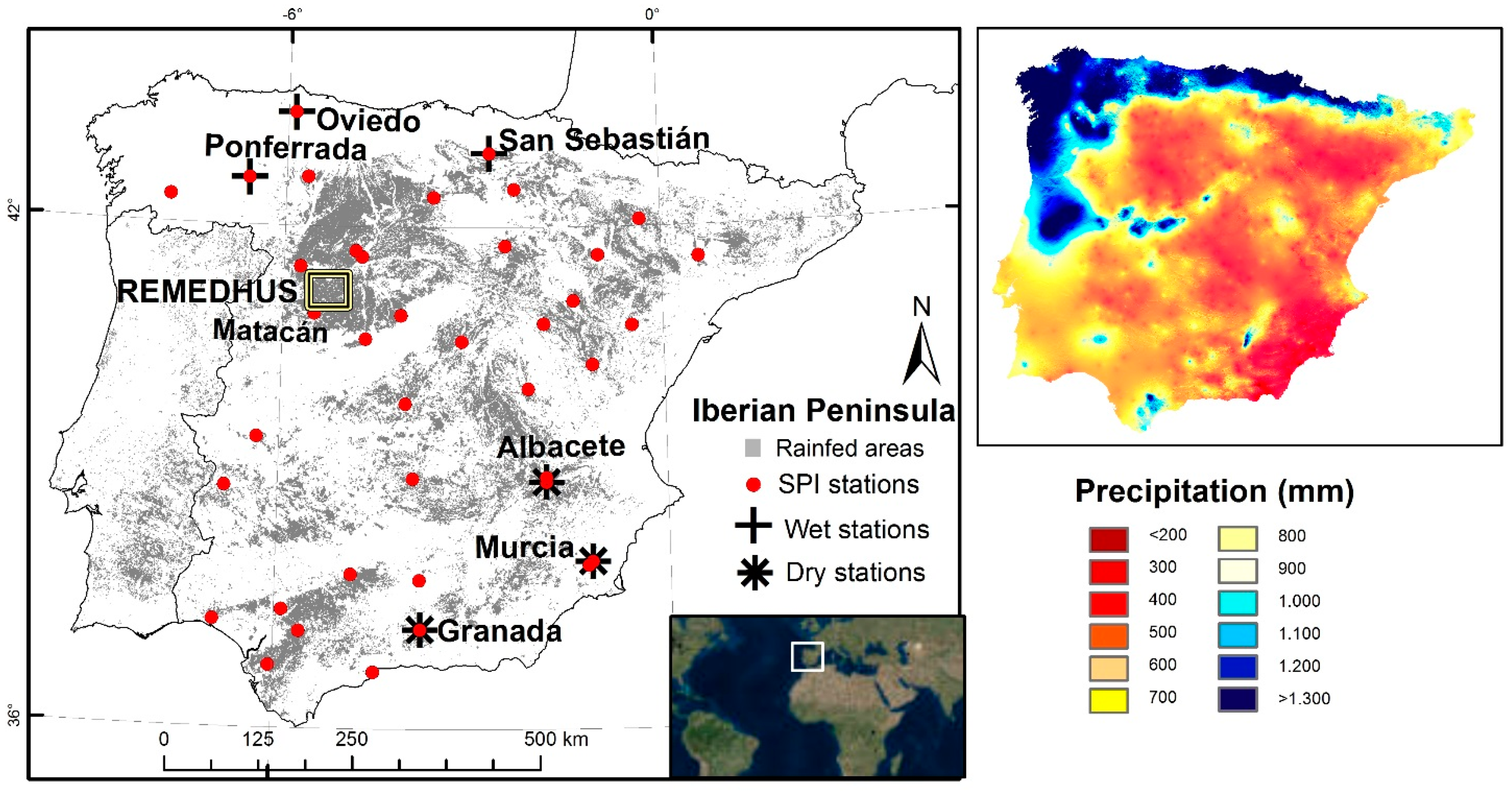
2.3. Climatic Conditions and Validation Strategies

SMADI assessment was conducted in two ways. First, it was compared with two agricultural drought indices, the Soil Water Deficit Index, SWDI [12] and the CMI, calculated both of them with in situ data from the soil moisture measurement stations network of the University of Salamanca, REMEDHUS, and the Spanish Meteorological Agency network, AEMet (Figure 1). Both indices were designed to evaluate short-term drought conditions across crop-producing regions. However, while the CMI is based on the mean temperature and total precipitation, the SWDI uses root zone soil water parameters. Note that, although both SWDI and SMADI use soil moisture as a key parameter, the first computes the soil moisture at the root zone (0–50 cm) whereas the latter considers only the first centimeters of the soil, as observed by SMOS.
SWDI and CMI were calculated from in situ soil moisture, climatic data and soil parameters [12]. Thus, they are totally independent from the remote sensing sources of SMADI. The climate of this region is continental semi-arid Mediterranean, with an average annual precipitation of 385 mm and a mean temperature of 12 °C [45]. Six stations of REMEDHUS were selected to compute the SWDI, whereas for the CMI calculation, the closest long-term weather station to REMEDHUS (Matacán, from the AEMet network) was used, which provided climatic series from more than 60 years. The temporal evolution of each version of SMADI was compared with SWDI at REMEDHUS (area-averaged) and with the CMI at the Matacán weather station (point-scale), using the Pearson correlation coefficient (R).
The second validation strategy is focused on the spatial and temporal occurrence of drought cases in the IP. Even though drought is a relative condition that differs widely between locations and climates, standardized indices like the SPI allow the user to confidently compare historical and current droughts between different climatic and geographic locations. SPI and SMADI series are compared at given selected locations to assess whether they provide valuable information about the spatial occurrence and time spans of drought events in the IP. The SPI was designed to quantify the precipitation deficit at multiple timescales, in order to reflect the impact of drought on the availability of the different water resources [60]. As soil moisture responds to precipitation anomalies on a relatively short scale, and since only short-term drought is investigated, the minimum timescale possible was chosen, which is one month. Smaller periods are not recommendable [61]. The one-month SPI may approximate conditions represented by the CMI [60] and is generally used to reflect short-term conditions related with short-term soil moisture and crop stress, especially during the growing season. Following the classification system to define drought thresholds [7], a drought event occurs any time the SPI is continuously negative and reaches an intensity of −1.0 or less, and ends when the SPI becomes positive. The monthly SPI at 39 locations of the IP were provided by the AEMet (http://www.aemet.es) based on the weather stations network distributed along the IP (Figure 1). Comparison of these series with SMADI allowed to assess the coincidence in time with those events as well as their intensity and duration. In this case, for the correlation analysis, the time interval should be taken into account. The SPI for this study is provided at a monthly basis, meaning that at a given month, SPI compares the total precipitation for that month in a particular year with the total precipitation of that month considering all the years of the time record. Hence, we assigned the monthly SPI value to the last day of each month to calculate the Pearson coefficient. This selection was in line with the guidelines of the EDO, which contrasts the SPI of a determinate month with the anomalies of soil moisture and vegetation of the last decade of this month.
Annual average rainfall in the IP shows a high spatial variability, ranging from less than 200 mm to above 1300 mm in average. In general, highest values are located in the Northern and Northwestern areas, and the lowest values were recorded in the Southeast of Spain.
The study period spans between January 2010 and December 2014. Based on the Joint Research Center (JRC) European Drought Observatory (EDO) monitoring of the occurrence and evolution of the drought events over Europe, as well as the AEMet, two periods were especially dry in several areas of the IP during this period. The most severe took place between October 2013 and July 2014, and was located at the Southeastern (the Murcia and Valencia regions, and Eastern Andalucía) and at the center of the IP, regions which were affected by mean and long-term precipitation deficits, leading to significant soil moisture deficits. This was considered by the JRC as an “exceptional drought” [62]. The persistent lack of rain in central and Southern Spain determined scarce soil moisture during the grain-filling phase of winter and spring crops. The situation worsened at the beginning of June when maximum daily temperatures increased above seasonal values leading to a critical early senescence [63]. Those regions were selected to analyze the performance of the new index.
The second severe period of drought occurred during 2012, a dry and warm year for the entire IP, but particularly stronger in the center and Northwestern part, where the precipitation deficit rendered a very dry year. Less marked, 2011 was also a dry year, more intensely for areas usually wet as the Northern part of Spain.
As opposed to drought periods, 2010 was very wet (even extremely wet in some areas) in the Southern part (30% more water than usual), leading to a surplus in the water reservoirs. Also the first trimester of 2013 was especially wet in the Northern and Western parts of the IP.
For qualitative comparison purposes, three locations were selected in the wet domain (Ponferrada, Oviendo and San Sebastián) and other three in the dry one (Albacete, Murcia and Granada), whereas the other area of study, comprising REMEDHUS, belongs to the dry domain (Figure 1).

3. Results and Discussion

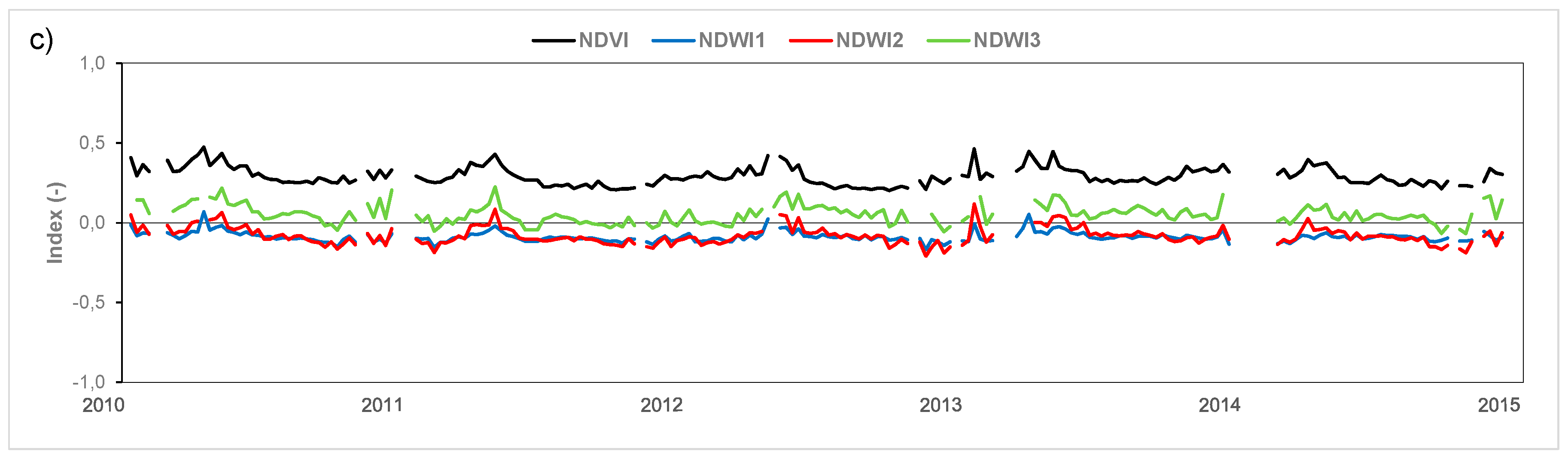
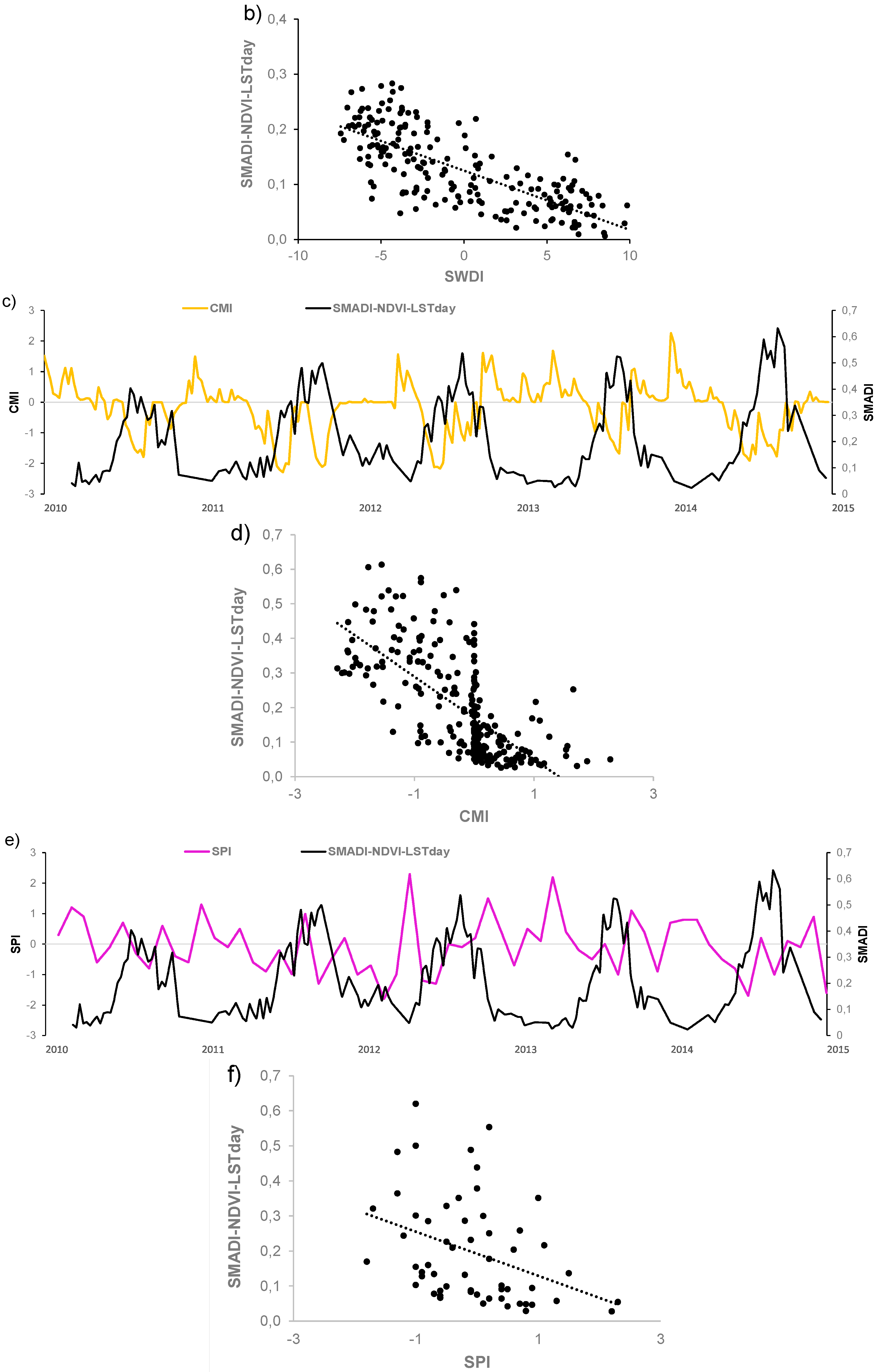
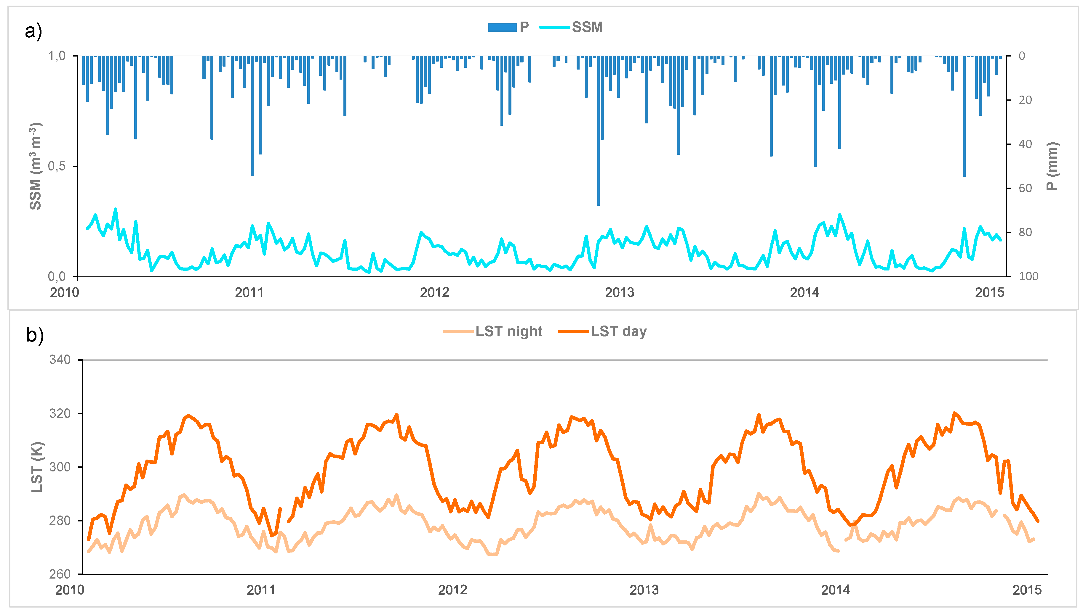
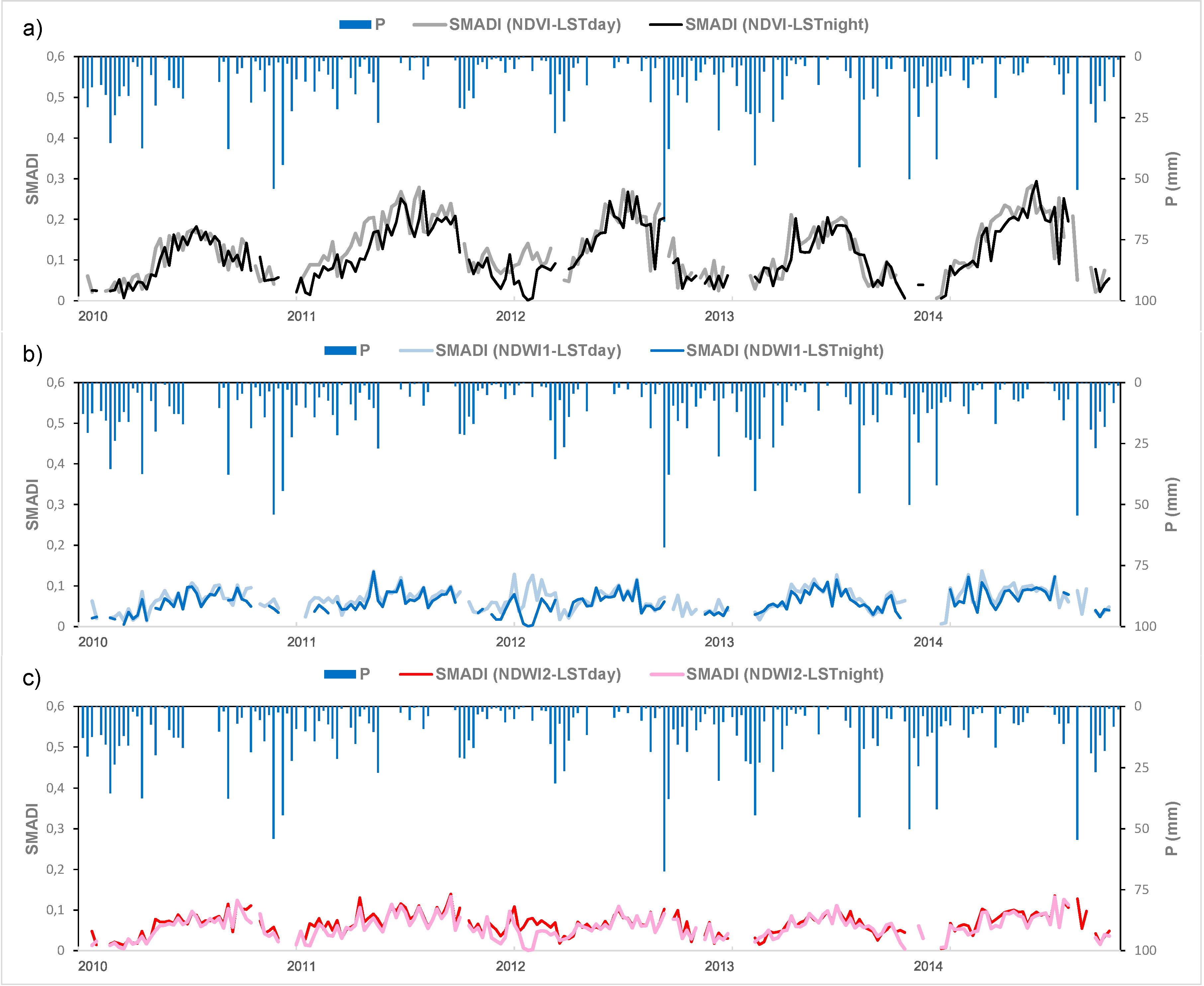
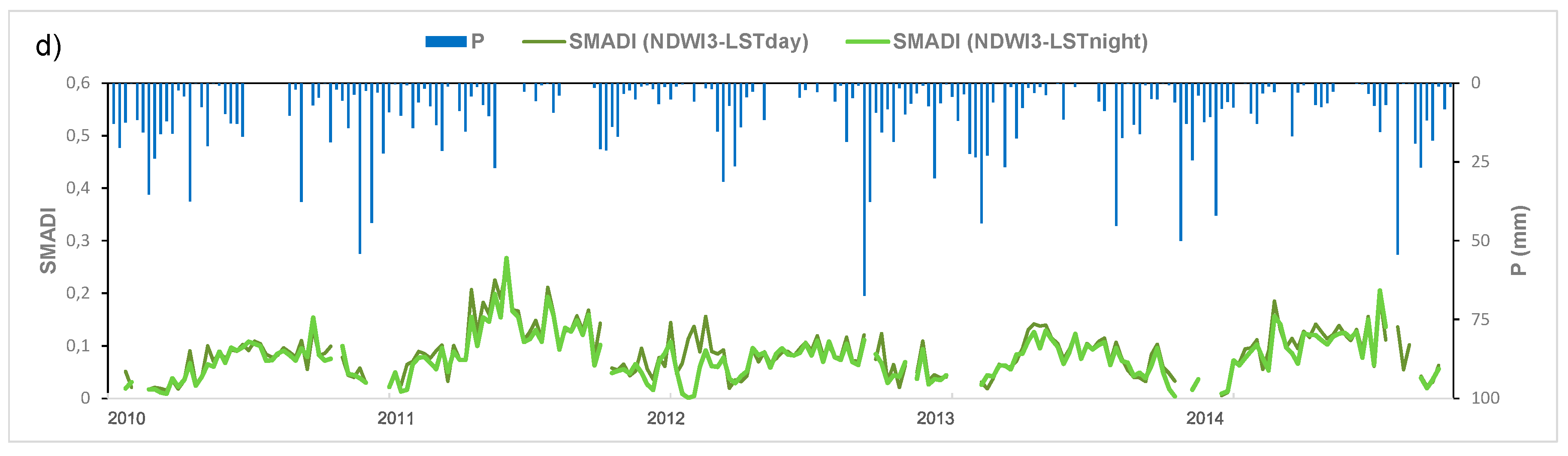
3.1. Evaluation at the REMEDHUS Area

The time evolution of the SMADI input parameters (LST, NDVI/NDWI and SSM) averaged over REMEDHUS are shown in Figure 2. It can be observed that both SSM and LST day/night curves showed a marked seasonality along the period (Figure 2a,b). As expected, the maximum temperature coincides with the smaller SSM in summer time, and the minimum temperature coincides with the maximum SSM in winter time. Also, LST exhibits smaller dynamic range for the night overpasses than the day ones. Regarding the vegetation-water indices (Figure 2c), NDVI exhibits the higher values, and all depict clear peaks in spring, during the growing season. NDWI1 and NDWI2 maintain negative values along the whole period excepting for the spring, consistent with the absence of vegetation water content out of the growing season.
Eight SMADI versions were calculated from the two alternatives of LST (day/night) and the four indices NDVI, NDWI1, NDW2 and NDWI3 (Figure 3). The NDVI-derived SMADI shows the highest dynamic range (0–0.3) and NDWI1 and NDW2 the lowest (0–0.1). Also, the four NDWI-derived SMADI resulted in a noisier or more instable curve than the NDVI one. All the SMADI versions showed a marked seasonality (Figure 3a–d), but the low values of NDWI 1 and 2 (Figure 2c) lead to unrealistic values of SMADI (Figure 3b,c). Comparing the annual cycles, only NDVI and NDWI3 allow discriminating year 2010 as the wettest year. Gu et al. [64] investigated the use of NDWI and NDVI for drought assessment over the U.S. Great Plains and found that NDWI was slightly more sensitive than NDVI to the initial onset and to the peak severity of drought conditions over grasslands. In the current research the vegetation variable is included as a descriptor of the vegetation status and vigor, but not as a proxy of drought itself. This could explain why the use of NDVI in the drought index was more effective than the use of the NDWI alternatives.
A series of eight-day SWDI were calculated at each REMEDHUS station using their specific soil parameters. Then the REMEDHUS average was computed and both series of SMADI and SWDI were statistically compared, resulting in statistically significant correlations ranging from −0.53 to −0.75 (Table 1, in grey). The negative correlation is due to the different description of drought using SWDI (negative values indicate drought conditions) and SMADI (positive values indicate drought conditions). In Table 1 the results of a sensitivity analysis considering different lags for the SMADI calculation were also shown. No lag, 16-day lag and 24-day lag were considered, as a way to test the feasibility of the 8-day lag suggested. From the obtained correlations several conclusions can be made. First, the best results were for the eight-day lag, as considered in the rationale of the index. On the contrary, the worst results came from the calculation using no lag at all, excepting in the case of the SMADI-NDVI version. Hence, it seemed recommendable to consider the lagged vegetation response to drought when using vegetation indices. Finally, it can be detected that in general, as the lag increased, the results worsened, making lags beyond 24 days doubtful.
Figure 4a,b show the time evolution and scatter plot of SWDI vs. the SMADI-NDVI-LST day (the case of highest correlations). Both indices show a marked seasonality and reveal the period from winter, 2011 to spring, 2012 as the driest of the series.
Since the SSM itself, the LST or the water/vegetation indices could also be potential indicators of drought, they were also compared to the SWDI over REMEDHUS (Table 2). High correlations were found between SWDI and LSTday, and SWDI with SSM, similar to those with SMADI (R ~ 0.75). On the contrary, very low correlations were obtained between SWDI and the water indices (R ~ 0.2). Similarly, the comparisons of the SMADI parameters taken separately with the drought indices SPI and CMI in Matacán (Table 2) exhibited good correlations with the LSTday and the SSM. These results indicate that SSM and LST information alone can be used to follow the water stress conditions, especially as described trough the SWDI and the CMI, at least under the semiarid conditions of the REMEDHUS area.
The next analysis compared SMADI vs. CMI and SPI (Table 3), all of them computed at the Matacán station. CMI and SMADI showed an inverse good correlation, being the NDVI alternative the best correlated. Taken into account that the CMI threshold depicting drought condition goes below −1 [8], only years 2011 and 2012 can be appointed as moderately dry years (during the summer period) with values of CMI between −1 and −2 (Figure 4c). However, CMI showed some drought breaks during the dry periods, especially in 2011, linked to small rainfall events, as also found in Martínez-Fernández et al. [12], but also the typical near-zero values at the beginning and ending of the growing season. Both facts limited its use as a long-term drought monitoring tool and outside the general growing season, as pointed out by the US National Drought Mitigation Center. Also, in the scatter plot of Figure 4d, it is shown that the correlation is lower when CMI>0, out of drought conditions.
For the SPI comparison (Table 3), the correlation worsened, although it was still statistically significant and remarkable given the very different source of SPI, as well as its different time scale as comparison of SMADI. Besides, SPI evolution had no seasonal patterns and there was no clear pattern of drought along the whole cycle (Figure 4e).

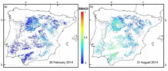
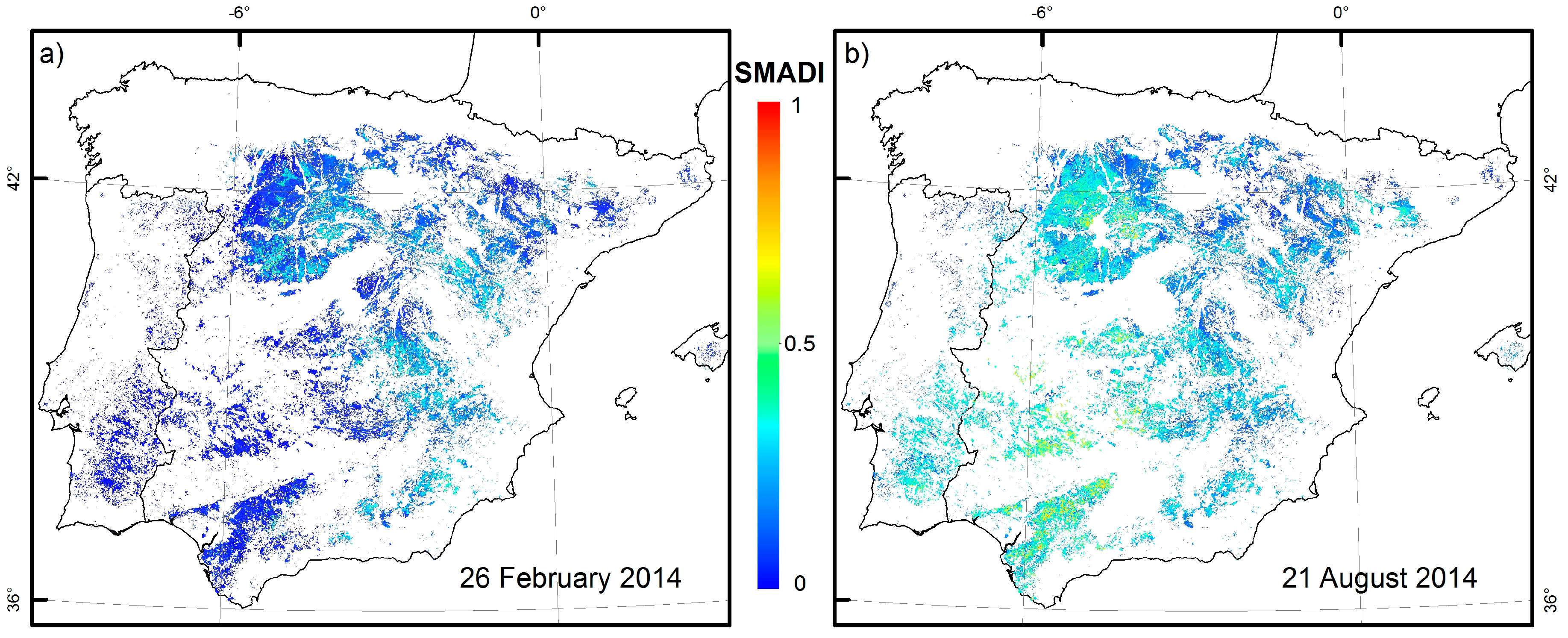
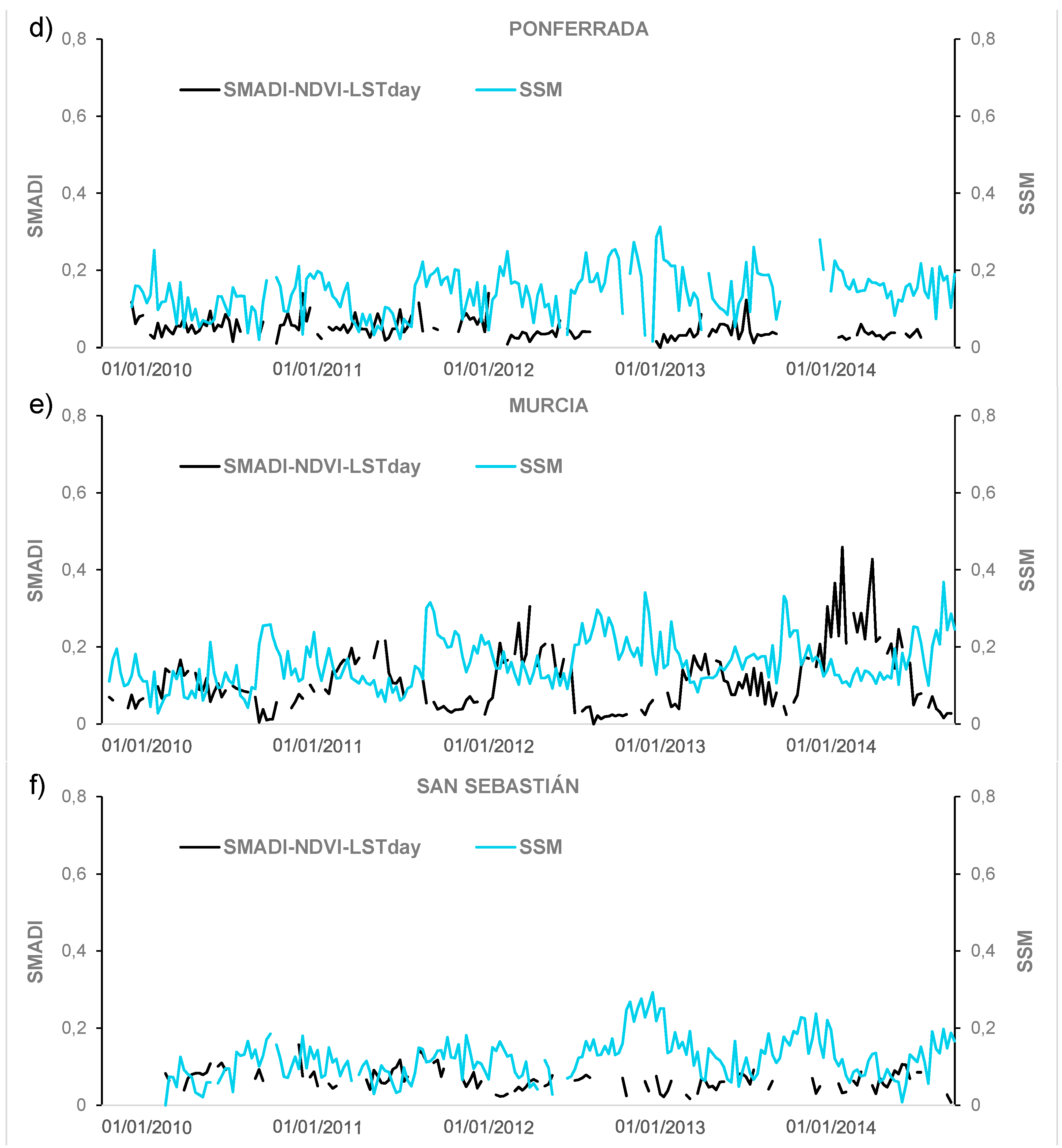
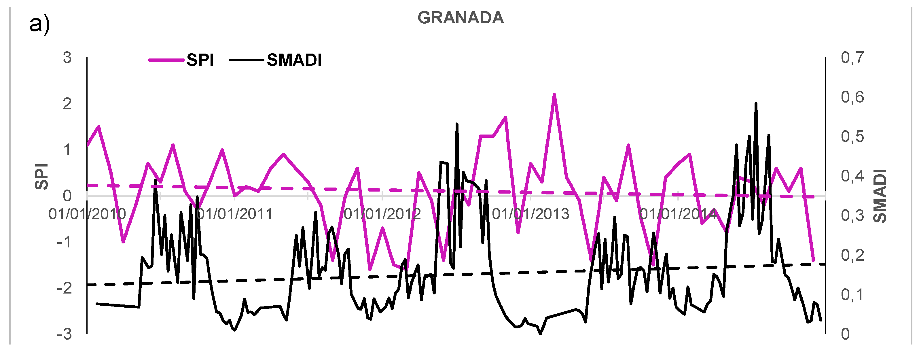
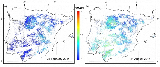
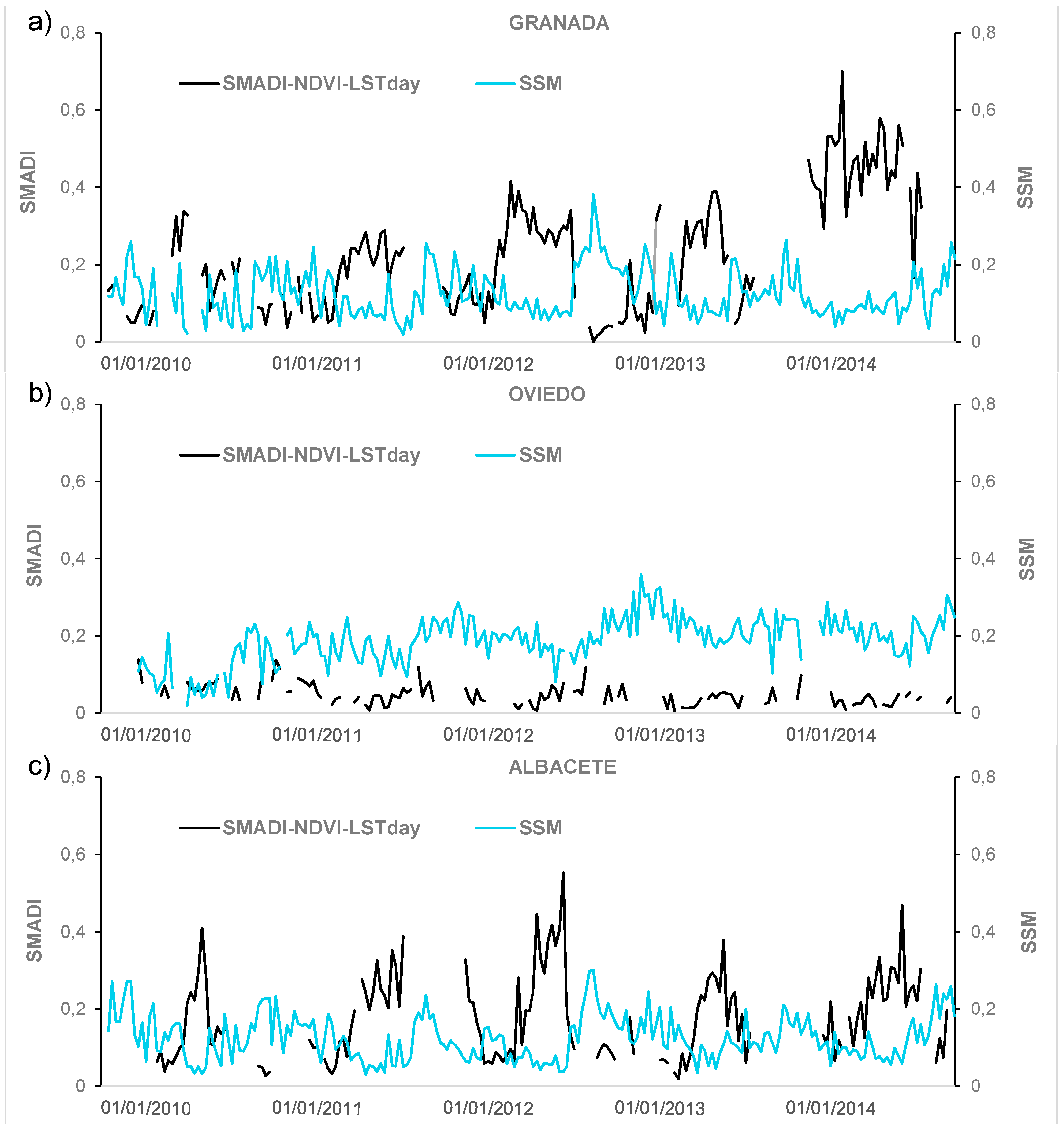
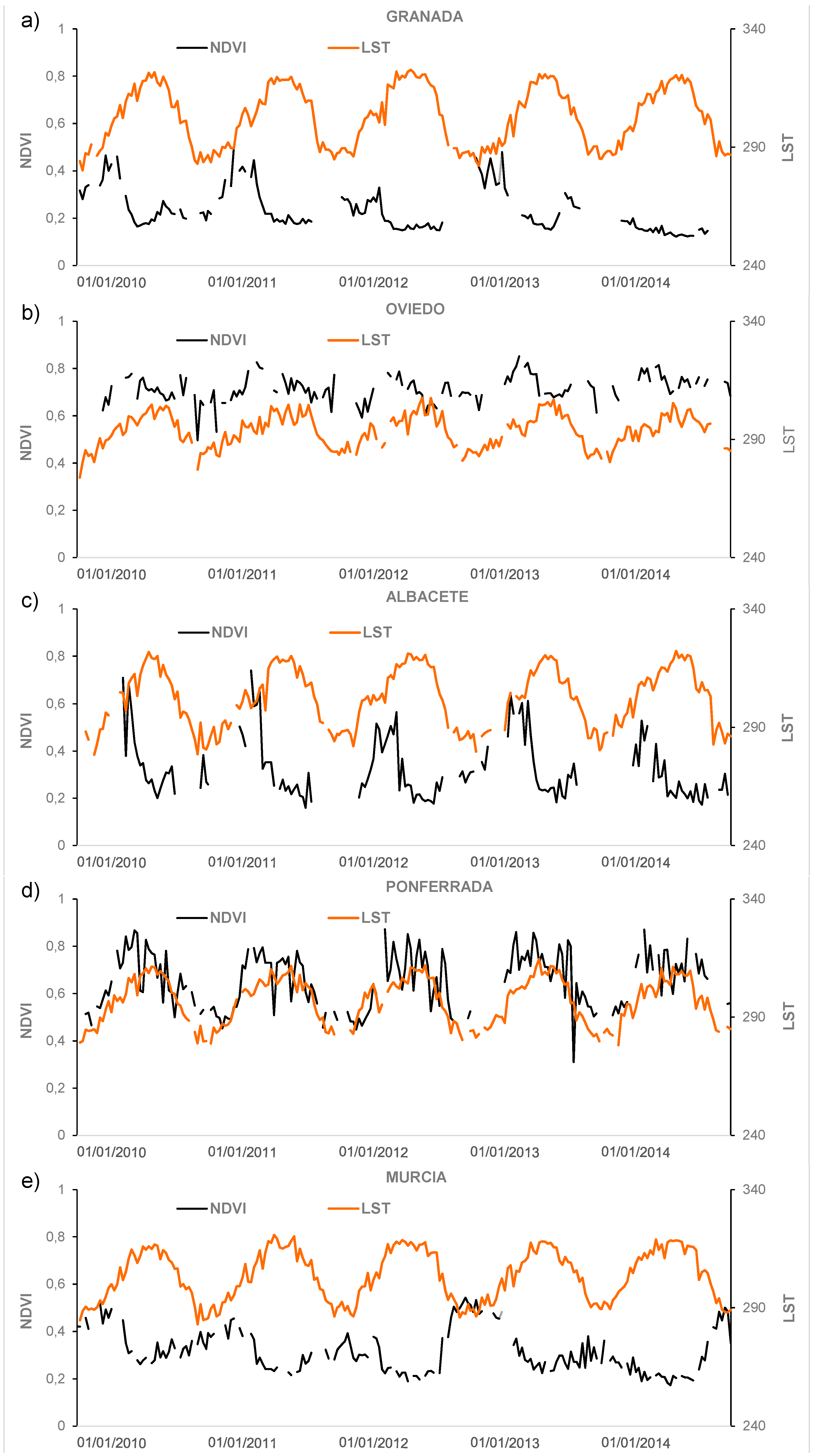
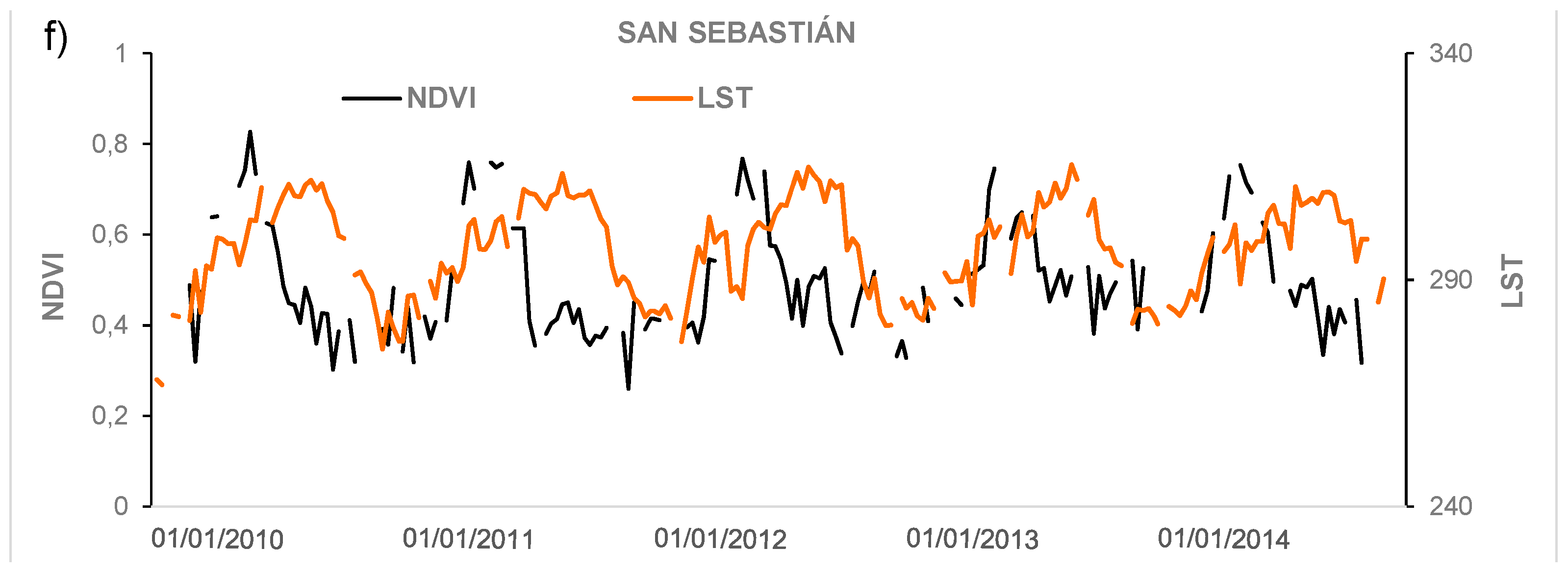
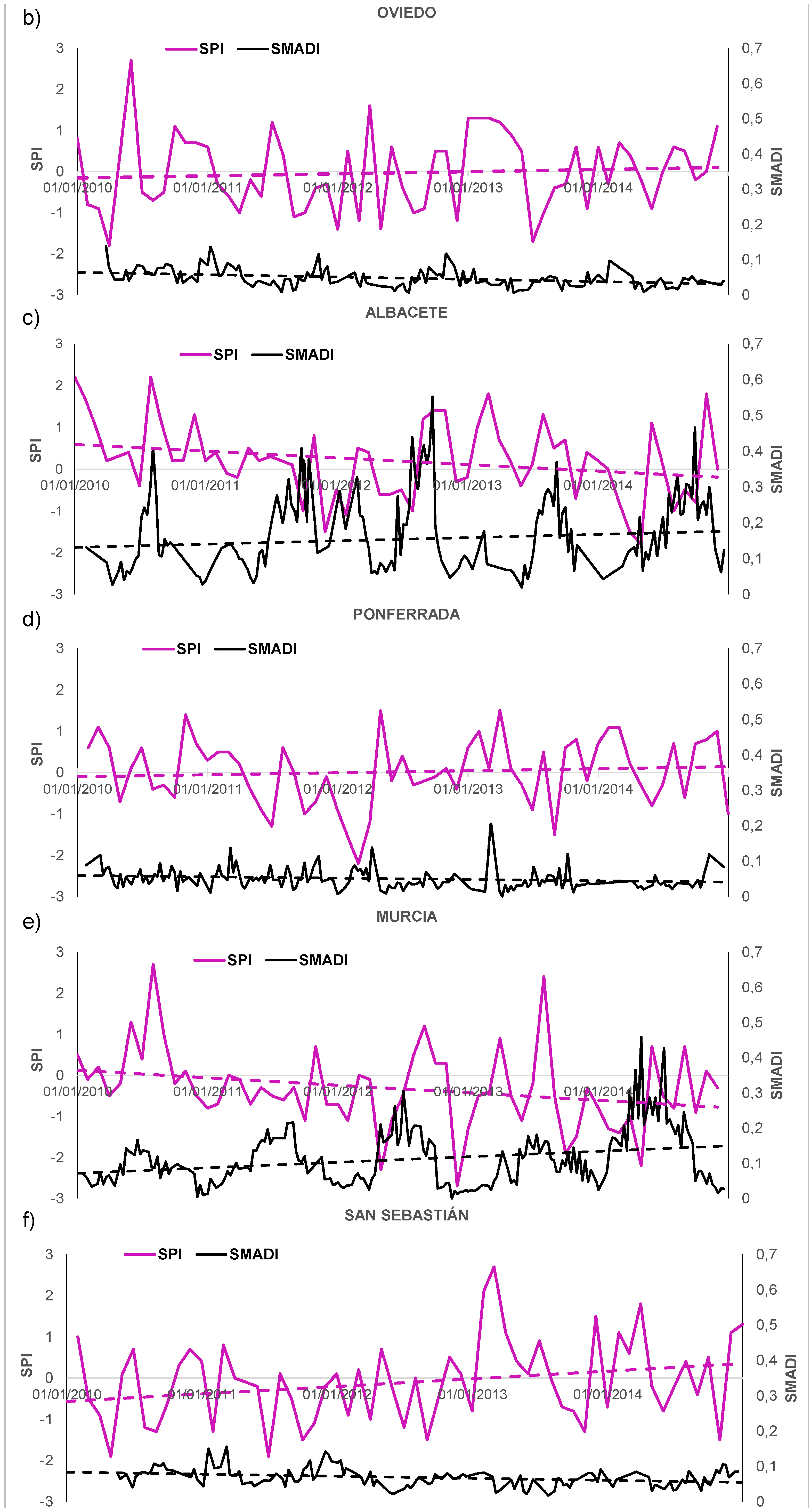
3.2. Evaluation over the Iberian Peninsula

Eight SMADI maps of the IP for each day and version resulted from the calculations (Figure 5, only NDVI-LSTday version is shown for brevity). To qualitatively verify the behavior of SMADI and its input parameters under other climatic conditions than that of the REMEDHUS area, three dry areas and three wet areas were selected in the Northwestern and Southeastern parts of the IP, respectively (Figure 1). The good performance of the SSM and LST shown in the previous section (Table 2) was tested under other bioclimatic conditions, with the aim to analyze whether the synergistic nature of SMADI reacts better to the extreme conditions than the parameters related to soil or vegetation taken individually. Thus, SMADI and SSM curves were extracted in areas belonging to the dry (Figure 6a,c,e) and wet (Figure 6b,d,f) domains. The comparison between the SSM in dry/wet areas suggested that since there were not notable differences between the SSM for dry/wet areas, SMADI was much higher for the dry areas, indicating drought conditions, especially in 2012 and 2014. These results are evidence that SMADI exhibits a higher potential to determine synoptic drought conditions than SSM information alone.
Besides, the LST and the NDVI were also extracted at the same six areas (Figure 7). The LST showed a marked seasonality in all cases, having a slightly smaller dynamic range and also slightly smaller maximum values in the wet areas. Furthermore, the NDVI exhibited much higher values for the wet areas (Figure 7b,d,f) than for the dry ones (Figure 7a,c,e). Thus it may be presumed that NDVI, which taken separately, showed no strength correlation with drought indices such as the SWDI, SPI and CMI (Table 2), is key to reflecting the response of crops to drought, as already suggested by Li et al. [57]. However, periods where NDVI is usually very depressed and the VCI has low values can be interpreted erroneously as a drought [46]. In such cases, the combination of VCI with MTCI and SMCI in SMADI provided the necessary information to distinguish drought from non-drought events. In other words, the information about the vegetation status provided by the vegetation index is essential to depict agricultural drought, but only when used jointly with the soil moisture status and the seasonal pattern provided by the LST.
A second temporal analysis consisted in the quantitative comparison of SMADI with the SPI via the correlation coefficient calculated at each AEMet station with SPI data available (n = 39). Nonetheless, it is important to keep in mind the different timing of both SPI and SMADI and their different approach. Moreover, SMADI used a shorter, 5 years-record of soil moisture instead of the long-term precipitation series used for the SPI (more than 40 years). Hence, not surprisingly the quantitative comparison of SPI with SMADI led to weak results. Only 9 stations showed significant correlations, beyond −0.40. Those discouraging results were also detected previously for the Matacán station (Figure 4e,f and Table 3). It could be suspected that owing to its nature of short-term-deviation from a normal value, the SPI correlation with products like anomalies of soil moisture should be higher, as found in Scaini et al. [65].
Figure 8 depicts the temporal evolution both of SPI and SMADI for the six dry/wet stations. The SPI temporal evolution is difficult to interpret. From a qualitative point of view, no seasonal patterns nor differences between dry/wet areas are noticeable. Also, no annual/seasonal patterns were found, and abnormally dry/wet months (−2 > SPI > 2) were found throughout the period. Typically, one-month SPI represents the percent of normal precipitation for a given month, i.e., positive SPI values indicate greater precipitation than the median (i.e., wet conditions), and negative values indicate less than median precipitation (i.e., dry conditions). The shorter the time scale of the SPI (typically one, three or 12 months), the more the SPI value moves above and below zero [7], as the deviation with respect to the mean precipitation of a given month is expected to be more variable than that of a year average. For example, in regions where rainfall is usually low during a month, as occurs in the IP during the dry season, SPI results can be misleading due to large negative or positive values resulting from relatively small departures from the median values.
A distinctive temporal trend resulted from the analysis of SPI and SMADI temporal evolution over the selected dry/wet areas (Figure 8). A clear increasing SMADI trend along the period 2010–2014 was found (Figure 8a,c,d), in close correspondence with a decreasing SPI trend (both indices have an opposite sense), the latter in a lesser extent. This trend was also found in half of the stations located in the dry domain. This pattern was not found in the input parameters of SMADI (Figure 7), thus it should not be attributed to a similar trend for the input parameters. On the contrary, all the stations under wet conditions in the IP showed no trend (Figure 8b,d,f), meaning no increase nor decrease of the drought conditions described trough SMADI along time. However, since only a few stations under the wet domain had concurrent SPI/SMADI data (Figure 1), these trends must be further analyzed with a longer data set and additional systematic criteria.

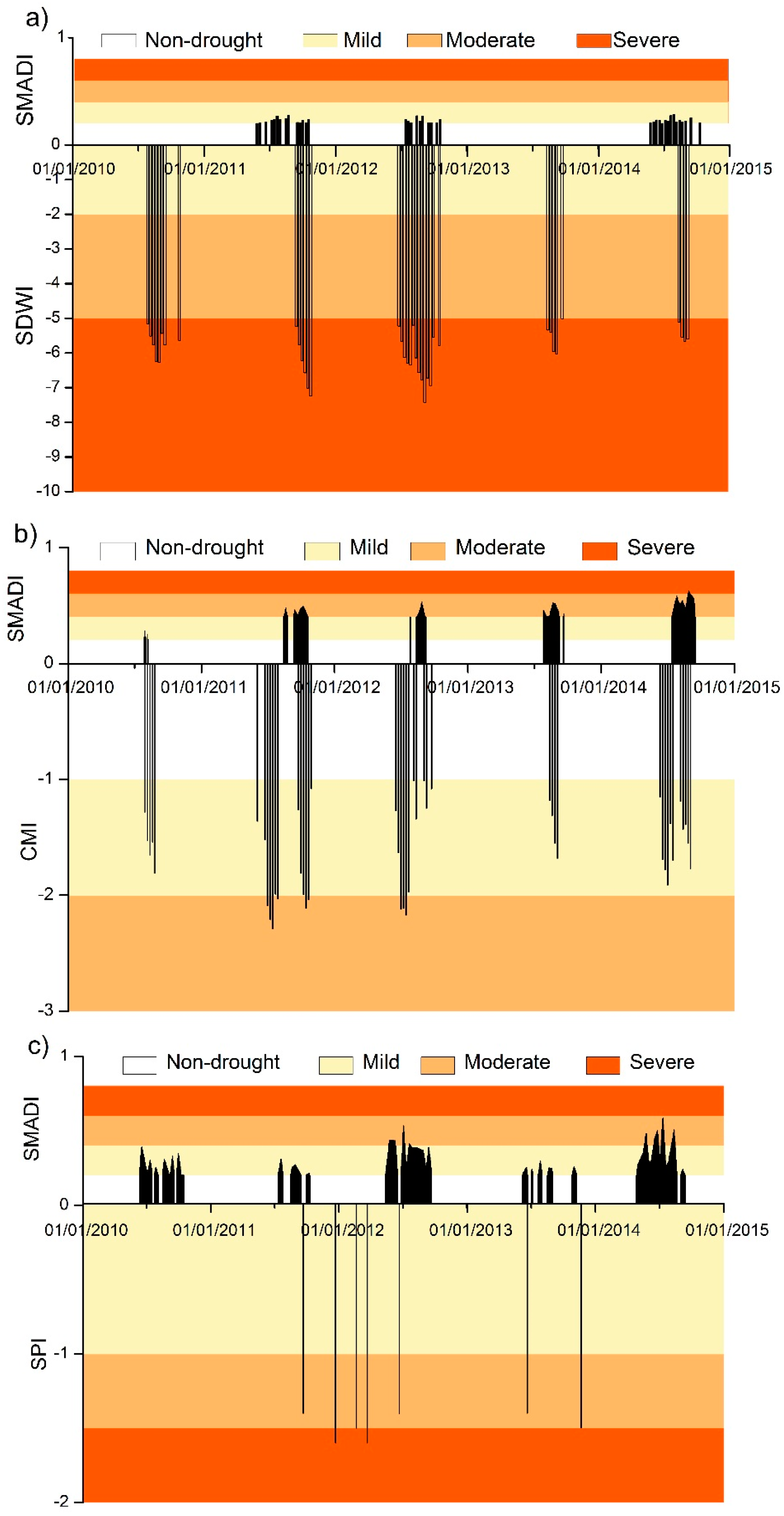
3.3. Functional Definition of Drought Using SMADI as Indicator

It is necessary to discuss the SMADI thresholds to consider drought periods/events, as well as their onset, duration and intensity. This is challenging given the multiple approaches and objectives of the drought analysis. One approach can be based on the comparison with current drought indices and their standardized ranges and classes to facilitate the comparison [39], i.e., adopting same number of classes and ranges as some standard classification like McKee et al. [7] for the SPI, in which seven categories from extremely wet to extreme drought where considered. When a vegetation surrogate of drought also based on a normal probability distribution is used, as the Standardized Vegetation Index [31], the classes try to mimic the SPI distribution. For SMADI, this approach is not applicable since the index is not based in a probabilistic function. Moreover, since SMADI is intended to depict abnormally low water supply for crops, but not extreme wet conditions, its range should span from normal, non-drought status to exceptional droughts. In this line, drought intensity categories, as used in the U.S. Drought Monitor and the EDO approaches, apply drought severity classification tables combining thresholds for each indicator for each dryness level. This would be the case of SMADI, which integrates the response of the vegetation (through VCI), LST (through MTCI) and SSM (through SMCI). One possible caveat of this approach is that different combinations of input indicators could mathematically lead to the same result. For example, it is expected that high values of SMADI, depicting moderate/severe drought scenarios, should come from a combination of unhealthy vegetation (very low VCI), soil moisture deficit (high SMCI) and high temperatures associated to thermal stress (high MTCI). However, Formula (10) may lead to the same SMADI values from various combinations of thresholds coming from vegetation, soil moisture and temperature only if their values are non-physical. In this regard, the rationale of SMADI, based on the LST/VI-SSM “universal triangle” ensures a realistic combination of these variables. Furthermore, the addition of the soil moisture condition from SMCI improves the uncertainties found from the additive combination of only vegetation and temperature, as proposed with VCI and TCI [27,46,66]. Semi-arid phenology seemed to be more dependent on moisture than temperature, as also found in [66]. As seen, temperature provides the seasonal pattern whereas the drought severity is governed by moisture supply. This improvement was shown in Figure 6 and Figure 7 under different climatic conditions. Unlike the approaches that include soil moisture as a measured or modelled parameter, SMADI integrates the near real time SMOS observations, which have already been successfully used as a drought indicator by itself [15,65,67]. The proposed ranges of the SMADI composite followed the principle of comparing the NDVI, LST and SSM of a particular year with the range of their variation during the extreme (stressed to favorable) conditions [68], but the combined use of these three indicators imposes a blended legend. SMADI results were normalized between 0 and 1, the first representing the favorable or normal conditions and the latter the extreme drought conditions. We propose five drought categories relying in the merged legend between the categories found in research alike [64,66,69,70], all of them based in turn in VCI, TCI or other NDVI-NDWI-based proxies, i.e., non-drought, abnormally dry (or mild drought), moderate drought, severe drought and extreme drought (Table 4). These categories are in accordance with standard drought indices ranges like SPI and the PDSI [8], but also with the soil-moisture based SWDI [12].
With these categories in mind, the duration and intensity of drought obtained with SMADI was compared to those resulting from SWDI and CMI at the REMEDHUS area and at the IP areas where SPI was available. Figure 9 shows a bar diagram representing drought events along the cycle (following thresholds and categories in Table 4) after SMADI (in top) and the other reference indices (SWDI at REMEDHUS, CMI at Matacán, and SPI at Granada) in the bottom, and a color scale depicting the intensity of drought. Overall, it can be noticed that the index that led to the most severe drought at the REMEDHUS stations is SWDI. The rest of indices barely reached moderate drought values at the Matacán station (CMI and SMADI) and few events of moderate drought in the Granada station, also a semiarid area, with the monthly SPI and SMADI. SWDI at REMEDHUS (Figure 9a) showed a remarkable seasonal pattern, leading to drought events in every summer from 2010 to 2014. In this case, SMADI seemed to be more conservative, since only years 2011, 2012 and 2014 showed periods considered as mild drought/abnormal dry. However, the duration of these dry spells are longer than those from SWDI in 2011 and 2014, and included the critical periods of the growing season (late May to July). It must be pointed out that those periods and intensities coincided with the outlook described in Section 2.3 from the AEMet and the EDO for this area. It should be mentioned that SMADI in REMEDHUS showed smaller impact of drought and fewer periods than Matacán (Figure 9b), even though they belong to the same area. A reason that could explain this lesser impact is that SMADI in REMEDHUS corresponds to a spatial average of the same six stations used for the SWDI study [12], whereas CMI was calculated at point scale on a single station.
The comparison of SMADI and CMI (Figure 9b) showed a good correspondence between the two indices, both in time and intensity, in line with results in Figure 4b,c. The durations of drought intervals were slightly longer for CMI, encompassing the whole growing season in 2011, 2012 and 2014 (as indicated by AEMet), pointing out the agricultural focus of this index. However, the degree of CMI was milder than SMADI, especially in 2014, where SMADI reached values of severity. As in REMEDHUS, SMADI considered 2010 under absence of drought, opposite to CMI and SWDI.
Finally, the comparison of SMADI vs. SPI in the Granada station (Figure 9c) showed an increase of the drought events length compared to the REMEDHUS area (Figure 9a,b), coinciding with the higher aridity of the Southeastern areas of the IP. Moreover, this increase can be especially distinguished in 2012 and 2014, the years where the harshest droughts occurred. Unlike SMADI, SPI showed drought values in winter and out of the growing season. However, the comparative analysis with SPI suffers from some caveats. First, it is a purely climatic indicator of drought, and the atmospheric processes are not always coupled with the soil-vegetation system, which is the basis of SMADI. Second, its monthly rate differs from the rest of indices making the comparison difficult, because a single value representative of an entire month should be assigned to a given date. Thus, the bad results of the time series correlation in Section 3.2 are not surprising.
The hypothesis of SMADI relies on the inverse relationship between LST and vegetation indices, i.e., high land surface temperatures can lead to soil moisture deficits and vegetation stress that characterize drought events. This assumption holds true for most parts of the world that are moisture-limited environments, but higher surface temperatures can actually be beneficial to vegetation growth in energy-limited environments (i.e., higher elevations and latitudes) [50,69]. Thus, other scenarios and climates should be analyzed to fully assess the SMADI performance, although several limitations of the SMOS soil moisture observations (e.g., mountain and coastal areas) can hinder a complete analysis.

4. Conclusions

A new agricultural drought indicator was presented based on the inverse relationship of surface temperature and vegetation status, which in turn is related to the soil moisture content. The new SMADI index is based on MODIS LST and NDVI/NDWI, together with SMOS SSM, all of them normalized after the maximum and minimum values across the five years of the study (2010–2015). Comparisons at local scale and over the IP were made, using other recognized drought indices over rainfed areas. The comparisons with CMI and SWDI at local scale in REMEDHUS showed a good agreement (R = −0.71 and −0.74, respectively), whereas the analysis with the monthly SPI at several locations in the IP was less satisfactory, probably due to its different time scale and nature. Furthermore, five categories of agricultural drought severity were proposed for SMADI following current classifications from other drought indicators, which permitted a description of drought conditions coherent with the European and Spanish drought observatories overview for the IP and study period. In comparison with other indices, SMADI was able to capture the drought events, their duration and intensity over the growing season. Further analysis of the proposed index, including the drought yield impact and an assessment over other climatic scenarios and land uses/covers are needed to fully evaluate its potential applications.
Among the SMADI variants, the best alternative resulted from the combination of SMOS with MODIS NDVI with LSTday, as proxies of the vegetation and temperature status, respectively. The inclusion of the vegetation-temperature binomial clearly improved the agricultural drought characterization based solely in soil moisture information. First, the addition of the vegetation proxy includes information on canopy vigor, closely related to the root zone water content, and complements the shallow depth of the SMOS SSM measurements. This effect should be carefully accounted for by the selection of an appropriate time lag between the plant response and the soil/climatic conditions, which in this study was set to 8 days. A plausible improvement could be to choose a variable lag along time, depending on the occurrence of extremely high temperatures, desiccating winds, low relative humidity, and the growing stage of the plants (i.e., a smaller lag is expected in the highest activity periods). Second, but equally important, SMADI allows combining SMOS coarse-scale and MODIS finer-scale information into an effective high resolution (500 m) product devoted to drought characterization and suitable for most practical applications.
The outcomes of this study suggest, in line with the most recent applications of remote soil moisture, that SMOS has good potential in monitoring agricultural drought, especially in synergy with optical and thermal imagery. With the forthcoming availability of microwave, optical and thermal data streams from new missions (SMAP, Sentinel-1 and -2), this study supports the development of innovative trails for enhanced drought monitoring and management services.

Acknowledgments

This study was supported by the Spanish Ministry of Economy and Competitiveness, MINECO (Projects AYA2012-39356-C05 and ESP2015-67549-C3-3) and the European Regional Development Fund, FEDER. Partial funding was also received from the BBVA Foundation. SPI and Matacán data were provided by the Spanish Meteorological Agency, AEMet. SMOS data was provided by the European Space Agency (Project AO-3230). MODIS products were retrieved from the NASA EOSDIS Land Processes Distributed Active Archive Center (LP DAAC), USGS/Earth Resources Observation and Science (EROS) Center.

Author Contributions

All authors contributed significantly to this research. The initial idea was conceived by Nilda Sánchez, and José Martínez-Fernández, María Piles and Ángel González-Zamora fully contributed to the design and development of the study. José Martínez-Fernández provided the field data and Ángel González-Zamora processed the field and satellite data. All the authors contributed to the interpretation of the results, participated in the manuscript and approved it.

Conflicts of Interest

The authors declare no conflict of interest.

References

  1. Moreira, E.E.; Mexia, J.T.; Pereira, L.S. Are drought occurrence and severity aggravating? A study on SPI drought class transitions using log-linear models and ANOVA-like inference. Hydrol. Earth Syst. Sci. Discuss. 2012, 16, 3011–3028. [Google Scholar] [CrossRef]
  2. Park, S.; Feddema, J.J.; Egbert, S.L. Impacts of hydrologic soil properties on drought detection with MODIS thermal data. Remote Sens. Environ. 2004, 89, 53–62. [Google Scholar] [CrossRef]
  3. Szép, I.J.; Mika, J.; Dunkel, J. Palmer drought severity index as soil moisture indicator: Physical interpretation, statistical behaviour and relation to global climate. Phys. Chem. Earth 2005, 30, 231–243. [Google Scholar] [CrossRef]
  4. Wilhite, D.A.; Glantz, M.H. Understanding the drought phenomenon: The role of definitions. Water Int. 1985, 10, 111–120. [Google Scholar] [CrossRef]
  5. Senay, G.B.; Budde, M.B.; Brown, J.F.; Verdin, J.P. Mapping flash drought in the U.S. Southern great plains. In Proceedings of the 22nd Conference on Hydrology, New Orleans, LA, USA, 20–24 January 2008.
  6. Hunt, E.D.; Hubbard, K.G.; Wilhite, D.A.; Arkebauer, T.J.; Dutcher, A.L. The development and evaluation of a soil moisture index. Int. J. Climatol. 2009, 29, 747–759. [Google Scholar] [CrossRef]
  7. McKee, T.B.; Doesken, N.J.; Kleist, J. The relationship of drought frequency and duration of time scales. In Proceedings of the Eighth Conference on Applied Climatology, Anaheim, CA, USA, 17–23 January 1993; pp. 179–186.
  8. Palmer, W.C. Meteorological Drought; Research Paper No. 45; Bureau, U.S.W., Ed.; NOAA Library and Information Services Division: Washington, DC, USA, 1965.
  9. Palmer, W.C. Keeping track of crop moisture conditions, nationwide: The new crop moisture index. Weatherwise 1968, 21, 156–161. [Google Scholar] [CrossRef]
  10. Wan, Z.; Wangab, P.; Lib, X. Using MODIS Land Surface Temperature and Normalized Difference Vegetation Index products for monitoring drought in the southern Great Plains, USA. Int. J. Remote Sens. 2004, 25, 61–72. [Google Scholar] [CrossRef]
  11. Ochsner, T.E.; Cosh, M.; Cuenca, R.H.; Dorigo, W.A.; Draper, C.S.; Hagimoto, Y.; Kerr, Y.; Njoku, E.G.; Small, E.E.; Zreda, M. State of the art in large-scale soil moisture monitoring. Soil Sci. Soc. Am. J. 2013, 77, 1888–1919. [Google Scholar] [CrossRef] [Green Version]
  12. Martínez-Fernández, J.; González-Zamora, A.; Sánchez, N.; Gumuzzio, A. A soil water based index as a suitable agricultural drought indicator. J. Hydrol. 2015, 522, 265–273. [Google Scholar] [CrossRef]
  13. Kerr, Y.; Waldteufel, P.; Wigneron, J.P.; Delwart, S.; Cabot, F.; Boutin, J.; Escorihuela, M.J.; Font, J.; Reul, N.; Gruhier, C.; et al. The SMOS MISSION: New tool for monitoring key elements of the Global Water Cycle. Proc. IEEE 2010, 98, 666–687. [Google Scholar] [CrossRef] [Green Version]
  14. Entekhabi, D.; Njoku, E.; O’Neill, P.E.; Kellogg, K.H.; Crow, W.T.; Edelstein, W.N.; Entin, J.K.; Goodman, S.D.; Jackson, T.; Johnson, J.; et al. The Soil Moisture Active Passive (SMAP) mission. Proc. IEEE 2010, 98, 704–716. [Google Scholar] [CrossRef]
  15. Chakrabarti, S.; Bongiovanni, T.; Judge, J.; Zotarelli, L.; Bayer, C. Assimilation of SMOS soil moisture for quantifying drought impacts on crop yield in agricultural regions. IEEE J. Sel. Top. Appl. Earth Obs. Remote Sens. 2014, 7, 3867–3879. [Google Scholar] [CrossRef]
  16. Carlson, T. Triangle models and misconceptions. Int. J. Remote Sens. Appl. 2013, 3, 155–158. [Google Scholar]
  17. Sánchez, N.; Martínez-Fernández, J.; Piles, M.; Camps, A.; Vall-llossera, M.; Aguasca, A. Hyperspectral-derived indices for soil moisture estimation at very high resolution. In Proceedings of the IEEE International Geoscience and Remote Sensing Symposium, IGARSS 2014, Québec, QC, Canada, 13–18 July 2014; pp. 2898–2901.
  18. Piles, M.; Sánchez, N.; Vall-llossera, M.; Camps, A.; Martínez-Fernández, J.; Martínez, J.; González-Gambau, V. A dowscaling approach for SMOS land observations: Evaluation of high resolution soil moisture maps over the Iberian Peninsula. IEEE J. Sel. Top. Appl. Earth Obs. Remote Sens. 2014, 7, 3845–3857. [Google Scholar] [CrossRef]
  19. Merlin, O.; Escorihuela, M.J.; Mayoral, M.A.; Hagolle, O.; Albitar, A.; Kerr, Y. Self-calibrated evaporation-based disaggregation of SMOS soil moisture: An evaluation study at 3 km and 100 m resolution in Catalunya, Spain. Remote Sens. Environ. 2013, 130, 25–38. [Google Scholar] [CrossRef] [Green Version]
  20. Thenkabail, P.S.; Gamage, M.S.D.N.; Smakhtin, V.U. The Use of Remote Sensing Data for Drought Assessment and Monitoring in Southwest Asia; International Water Management Institute: Colombo, Sri Lanka, 2004; p. 34. [Google Scholar]
  21. Reed, B.C. Using remote sensing and Geographic Information Systems for analyzing landscape/drought interaction. Int. J. Remote Sens. 1993, 14, 3489–3503. [Google Scholar] [CrossRef]
  22. Rundquist, B.C.; Harrington, J.A., Jr. The effects of climatic factors on vegetation dynamics of tallgrass and shortgrass cover. GeoCarto Int. 2000, 15, 31–36. [Google Scholar] [CrossRef]
  23. Wang, J.; Price, K.P.; Rich, P.M. Spatial patterns of NDVI in response to precipitation and temperature in the central Great Plains. Int. J. Remote Sens. 2001, 22, 3827–3844. [Google Scholar] [CrossRef]
  24. Farrar, T.J.; Nicholson, S.E.; Lare, A.R. The influence of soil type on the relationships between NDVI, rainfall and soil moisture in semiarid Botswana. II. NDVI response to soil moisture. Remote Sens. Environ. 1994, 50, 121–133. [Google Scholar] [CrossRef]
  25. Tucker, C.J.; Choudhury, B.J. Satellite remote sensing of drought conditions. Remote Sens. Environ. 1987, 23, 243–251. [Google Scholar] [CrossRef]
  26. Bayarjargal, Y.; Karnieli, A.; Bayasgalan, M.; Khudulmur, S.; Gandush, C.; Tucker, C.J. A comparative study of NOAA-AVHRR derived drought indices using change vector analysis. Remote Sens. Environ. 2006, 105, 9–22. [Google Scholar] [CrossRef]
  27. Bhuiyan, C.; Singh, R.P.; Kogan, F.N. Monitoring drought dynamics in the Aravalli region (India) using different indices based on ground and remote sensing data. Int. J. Appl. Earth Obs. Geoinf. 2006, 8, 289–302. [Google Scholar] [CrossRef]
  28. Kogan, F.N. Global drought watch from space. Bull. Am. Meteorol. Soc. 1997, 78, 621–636. [Google Scholar] [CrossRef]
  29. Hayes, M.J.; Decker, W.L. Using satellite and real-time weather data to predict maize production. Int. J. Biometeorol. 1998, 42, 10–15. [Google Scholar] [CrossRef]
  30. Kogan, F.N. Remote sensing of weather impacts on vegetation in nonhomogeneous areas. Int. J. Remote Sens. 1990, 11, 1405–1419. [Google Scholar] [CrossRef]
  31. Peters, A.J.; Walter-Shea, E.A.; Ji, L.; Viña, A.; Hayes, M.; Svoboda, M.D. Drought Monitoring with NDVI-Based Standardized Vegetation Index. Photogramm. Eng. Remote Sens. 2002, 68, 71–75. [Google Scholar]
  32. Wilhite, D.A. Drought monitoring, mitigation and preparedness in the U.S.: An end to end approach. In Proceedings of the WMO Task Force on Social-Economic Application of Public Weather Services, Geneva, Switzerland, 15–18 May 2006.
  33. WMO. Monitoring, Assessment and Combat of Drought and Desertification; World Meteorological Organization: Geneva, Switzerland, 1992; p. 111. [Google Scholar]
  34. Sivakumar, M.V.K. Agricultural Drought-WMO Perspectives. In Agricultural Drought Indices, Proceedings of the WMO/UNISDR Expert Group Meeting on Agricultural Drought Indices, Murcia, Spain, 2–4 June 2010; Sivakumar, M.V.K., Motha, R.P., Wilhite, D.A., Wood, D.A., Eds.; World Meteorological Organization: Geneva, Switzerland, 2011; Volume 1572, pp. 22–34. [Google Scholar]
  35. Sánchez-Ruiz, S.; Piles, M.; Sánchez, N.; Martínez-Fernández, J.; Vall-llossera, M.; Camps, A. Combining SMOS with visible and near/shortwave/thermal infrared satellite data for high resolution soil moisture estimates. J. Hydrol. 2014, 516, 273–283. [Google Scholar] [CrossRef]
  36. Ji, L.; Peters, A.P. Assessing vegetation response to drought in the northern Great Plains using vegetation and drought indices. Remote Sens. Environ. 2003, 87, 85–98. [Google Scholar] [CrossRef]
  37. Whiting, M.L.; Li, L.; Ustin, S.L. Predicting water content using Gaussian model on soil spectra. Remote Sens. Environ. 2004, 89, 535–552. [Google Scholar] [CrossRef]
  38. Lobell, D.B.; Asner, G.P. Moisture effects on soil reflectance. Soil Sci. Soc. Am. J. 2002, 66, 722–727. [Google Scholar] [CrossRef]
  39. Ezzine, H.; Bouziane, A.; Ouazar, D. Seasonal comparisons of meteorological and agricultural droughtindices in Morocco using open short time-series data. Int. J. Appl. Earth Obs. Geoinf. 2014, 26, 36–48. [Google Scholar] [CrossRef]
  40. Rouse, J.W.; Haas, R.H.; Shell, J.A.; Deering, D.W.; Harlan, J.C. Monitoring the Vernal Advancement of Retrogradation of Natural Vegetation; Final Report, Type III; NASA/GSFC: Greenbelt, MD, USA, 1974; p. 371.
  41. Gao, B. NDWI-A Normalized Difference Water Index for remote sensing of vegetation liquid water from space. Remote Sens. Environ. 1996, 58, 257–266. [Google Scholar] [CrossRef]
  42. Ayars, J.E. Adapting irrigated agriculture to drought in the San Joaquin Valley of California. In Drought in Arid and Semi-Arid Regions; Schwabe, K., Albiac, J., Connor, J.D., Hassan, R.M., Meza González, L., Eds.; Springer Netherlands: Dordrecht, The Netherlands, 2013; pp. 25–39. [Google Scholar]
  43. AEMet. Iberian Climate Atlas, 1971–2000; Agencia Estatal de Meteorología, Ministerio de Medio Ambiente y Medio Rural y Marino, Instituto de Meteorologia de Portugal: Madrid, Spain, 2011; p. 80.
  44. Ninyerola, M.; Pons, X.; Roure, J.M. Atlas Climático Digital de la Península Ibérica. Metodología y Aplicaciones en Bioclimatología y Geobotánica; Universidad Autónoma de Barcelona: Barcelona, Spain, 2005. [Google Scholar]
  45. González-Zamora, A.; Sanchez, N.; Martínez-Fernández, J.; Gumuzzio, A.; Piles, M.; Olmedo, E. Long-term SMOS soil moisture products: A comprehensive evaluation across scales and methods in the Duero Basin (Spain). Phys. Chem. Earth 2015, 83–84, 123–136. [Google Scholar] [CrossRef]
  46. Kogan, F.N. Application of vegetation index and brightness temperature for drought detection. Adv. Space Res. 1995, 11, 91–100. [Google Scholar] [CrossRef]
  47. Kogan, F.N.; Usa, D.C.; Stark, R.; Gitelson, A.; Jargalsaikhan, L.; Dugarjav, C.; Tsoojd, S. Derivation of pasture biomass in Mongolia from AVHRRbased vegetation health indices. Int. J. Remote Sens. 2004, 25, 2889–2896. [Google Scholar] [CrossRef]
  48. Goetz, S.J. Multisensor analysis of NDVI, surface temperature and biophysical variables at a mixed grassland site. Int. J. Remote Sens. 1997, 18, 71–94. [Google Scholar] [CrossRef]
  49. Sandholt, I.; Rasmussen, K.; Andersen, J. A simple interpretation of the surface temperature/vegetation index space for assessment of surface moisture status. Remote Sens. Environ. 2002, 79, 213–224. [Google Scholar] [CrossRef]
  50. Karnieli, A.; Agam, N.; Pinker, R.T.; Anderson, M.; Imhoff, M.L.; Gutman, G.G.; Panov, N.; Goldberg, A. Use of NDVI and land surface temperature for drought assessment: Merits and limitations. J. Clim. 2010, 23, 618–633. [Google Scholar] [CrossRef]
  51. McVicar, T.R.; Bierwirth, P.N. Rapidly assessing 1997 drought in Papua New Guinea using composite AHVRR imagery. Int. J. Remote Sens. 2001, 22, 2109–2128. [Google Scholar] [CrossRef]
  52. Nemani, R.R.; Pierce, L.; Running, S.W.; Goward, S.N. Developing satellite-derived estimates of surface moisture status. J. Appl. Meteorol. 1993, 32, 548–557. [Google Scholar] [CrossRef]
  53. Di, L.; Rundquist, B.C.; Han, L. Modeling relationship between NDVI and precipitation during vegetative growth cycles. Int. J. Remote Sens. 1994, 15, 2121–2136. [Google Scholar] [CrossRef]
  54. Zhang, F.; Zhang, L.W.; Wang, X.Z.; Hung, J.F. Detecting agro-droughts in Southwest of China using MODIS satellite data. J. Integr. Agric. 2013, 12, 159–168. [Google Scholar] [CrossRef]
  55. Anderson, W.B.; Zaitchik, B.F.; Hain, C.R.; Anderson, M.C.; Yilmaz, M.T.; Mecikalski, J.; Schultz, L. Towards an integrated soil moisture drought monitor for East Africa. Hydrol. Earth Syst. Sci. 2012, 16, 2893–2913. [Google Scholar] [CrossRef]
  56. Schnur, M.T.; Xie, H.; Wang, X. Estimating root zone soil moisture at distant sites using MODIS NDVI and EVI in a semi-arid region of southwestern USA. Ecol. Inform. 2010, 5, 400–409. [Google Scholar] [CrossRef]
  57. Li, R.; Tsunekawa, A.; Tsubo, M. Index-based assessment of agricultural drought in a semi-arid region of Inner Mongolia, China. J. Arid Land 2014, 6, 3–15. [Google Scholar] [CrossRef]
  58. Nghiem, S.V.; Wardlow, B.D.; Allured, D.; Svoboda, M.D.; LeComte, D.; Rosencrans, M.; Chan, S.K.; Neumann, G. Microwave Remote Sensing of Soil Moisture. In Remote Sensing of Drought: Innovative Monitoring Approaches; Wardlow, B.D., Anderson, M.C., Verdin, J.P., Eds.; CRC Press: Boca Raton, FL, USA, 2012; pp. 197–226. [Google Scholar]
  59. Higgins, R.W.; Shi, W.; Yarosh, E.; Joyce, R. Improved United States precipitation quality control system and analysis. In NCEP/Climate Prediction Center Atlas; Climate Prediction Center: Camp Springs, MD, USA, 2000; Volume 7, p. 40. [Google Scholar]
  60. WMO. Standardized Precipitation Index. User Guide; World Meteorological Organization: Geneva, Switzerland, 2012; p. 24. [Google Scholar]
  61. Wu, H.; Svoboda, M.D.; Hayes, M.J.; Wilhite, D.A.; Wen, F. Appropriate application of the Standardized Precipitation Index in arid locations and dry seasons. Int. J. Climatol. 2007, 27, 65–79. [Google Scholar] [CrossRef]
  62. EC-JCR; European Drought Observatory (EDO). Drought News 2014; European Drought Observatory: Ispra, Italy, 2014; p. 8. [Google Scholar]
  63. EC-JCR. Crop Monitoring in Europe; AGRI4CAST-JRC/IES MARS Unit: Luxembourg, 2014; p. 44. [Google Scholar]
  64. Gu, Y.; Brown, J.F.; Verdin, J.P.; Wardlow, B.D. A five-year analysis of MODIS NDVI and NDWI for grassland drought assessment over the central Great Plains of the United States. Geophys. Res. Lett. 2007, 34, L06407. [Google Scholar] [CrossRef]
  65. Scaini, A.; Sánchez, N.; Vicente-Serrano, S.M.; Martínez-Fernández, J. SMOS-derived soil moisture anomalies and drought indices: A comparative analysis using in situ measurements. Hydrol. Processes 2015, 29, 373–383. [Google Scholar] [CrossRef]
  66. Bhuiyan, C. Desert vegetation during droughts: Response and sensitivity. Int. Arch. Photogramm. Remote Sens. Spat. Inf. Sci. 2008, 21, 907–912. [Google Scholar]
  67. Martínez Fernández, J.; González- Zamora, A.; Sánchez, N.; Gumuzzio, A.; Herrero-Jiménez, C.M. Satellite soil moisture for agricultural drought monitoring: Assessment of the SMOS derived Soil Water Deficit Index. Remote Sens. Environ. 2016, 177, 277–286. [Google Scholar] [CrossRef]
  68. Kogan, F. Operational space technology for global vegetation assessment. Bull. Am. Meteorol. Soc. 2001, 82, 1949–1964. [Google Scholar] [CrossRef]
  69. Sivakumar, M.V.K.; Stone, R.; Sentelhas, P.C.; Svoboda, M.; Omondi, P.; Sarkar, J.; Wardlow, B. Agricultural drought indices: Summary and recommendations. In Agricultural Drought Indices, Proceedings of the WMO/UNISDR Expert Group Meeting on Agricultural Drought Indices, Murcia, Spain, 2–4 June 2010; Sivakumar, M.V.K., Motha, R.P., Wilhite, D.A., Wood, D.A., Eds.; World Meteorological Organization: Geneva, Switzerland, 2011; Volume 1572, pp. 172–194. [Google Scholar]
  70. Brown, J.F.; Wardlow, B.D.; Tadesse, T.; Hayes, M.J.; Reed, B.C. The Vegetation Drought Response Index (VegDRI): An integrated approach for monitoring drought stress in vegetation. GIScience Remote Sens. 2008, 45, 16–46. [Google Scholar] [CrossRef]
  71. NOAA-National Weather Service. Available online: http://www.cpc.ncep.noaa.gov/products/analysis_monitoring/cdus/palmer_drought/wpdanote.shtml (accessed on 18 October 2015).
Figure 1. Spanish Meteorological Agency (AEMet) weather stations overlapping the rainfed domain map (n = 39) in which SPI is available. Map of the average annual precipitation is also shown [43,44], as well as the area of the soil moisture measurement stations network of the University of Salamanca, REMEDHUS.
Remotesensing 08 00287 g001
Figure 2. Temporal cycle of the input parameters: (a) SSM; (b) LST; (c) NDVI and NDWI for the REMEDHUS average during the study period (years 2010 to 2015).
Remotesensing 08 00287 g002aRemotesensing 08 00287 g002b
Figure 3. SMADI results at the REMEDHUS scale for (a) NDVI; (b) NDWI1; (c) NDWI2 and (d) NDWI3 versions.
Remotesensing 08 00287 g003aRemotesensing 08 00287 g003b
Figure 4. (af) Comparative evolution between SMADI (NDVI and LST day version) and the SWDI at the REMEDHUS area average (a); the CMI at the Matacán station (c) and the SPI at the Matacán station (e). Scatter plot of series correspond to (b,d,f), respectively.
Remotesensing 08 00287 g004aRemotesensing 08 00287 g004b
Figure 5. (a) SMADI maps (NDVI-LSTday version) for DoY = 57 (wet period) and (b) DoY = 233 (dry period).
Remotesensing 08 00287 g005
Figure 6. (af) Temporal evolution of SMADI and SSM at three dry (a,c,e) and wet (b,d,f) locations. Only the NDVI-LST day version was shown.
Remotesensing 08 00287 g006aRemotesensing 08 00287 g006b
Figure 7. (af) Temporal evolution of NDVI-LST at three dry (a,c,e) and wet (b,d,f) locations. Only the NDVI-LSTday version was shown.
Remotesensing 08 00287 g007aRemotesensing 08 00287 g007b
Figure 8. (af) Temporal evolution of SMADI and SPI at three dry (a,c,e) and wet (b,d,f) locations. Only the NDVI-LST day version was shown.
Remotesensing 08 00287 g008aRemotesensing 08 00287 g008b
Figure 9. Range and duration of the drought events following the different approaches of SMADI and SWDI in REMEDHUS (a); SMADI and CMI in Matacán (b); and SPI and SMADI in a dry-considered station at the IP, Granada (c).
Remotesensing 08 00287 g009
Table 1. Comparison (Pearson coefficient) between SWDI and SMADI at the REMEDHUS area average. Results using lags of 0, 16 and 24 days were also considered. All the correlations have a p-value < 0.01.
RSMADI-NDVISMADI-NDW1SMADI-NDW2SMADI-NDW3
LSTdayLSTnightLSTdayLSTnightLSTdayLSTnightLSTdayLSTnight
SWDI (REMEDHUS)−0.75−0.72−0.57−0.53−0.66−0.60−0.53−0.53
SWDI (REMEDHUS) 0 days lag−0.71−0.66−0.45−0.48−0.58−0.57−0.50−0.40
SWDI (REMEDHUS) 16 days lag−0.75−0.68−0.49−0.47−0.66−0.60−0.56−0.45
SWDI (REMEDHUS) 24 days lag−0.68−0.65−0.40−0.50−0.65−0.62−0.54−0.47
Table 2. Comparison (Pearson coefficient) between SWDI and the SMADI input parameters (LST, NDVI, NDWI and SSM) at the REMEDHUS area average and at the Matacán station. All the correlations have a p-value < 0.01.
RLSTdayLSTnightNDVINDWI1NDWI2NDWI3SSM
SWDI (REMEDHUS)−0.74−0.680.570.210.230.180.75
CMI (Matacán)−0.71−0.630.430.280.210.350.71
SPI (Matacán)−0.40−0.230.190.230.270.350.61
Table 3. Comparison (Pearson coefficient) between CMI and SMADI at the Matacán station. All the correlations have a p-value < 0.01.
RSMADI-NDVISMADI-NDW1SMADI-NDW2SMADI-NDW3
LSTdayLSTnightLSTdayLSTnightLSTdayLSTnightLSTdayLSTnight
CMI (Matacán)−0.71−0.69−0.44−0.45−0.33−0.34−0.36−0.39
SPI (Matacán)−0.37−0.33−0.41−0.25−0.26−0,19−0.28−0.22
Table 4. Drought categories after several indicators.
SWDICMI *SPI **PDSI ***SMADIDescription
0 or more0.9 to −0.991 to −0.99−0.49 or more0 to 0.19Normal, near normal, non-drought
0 to −1.99−1 to −1.99−0.5 to −1.990.20 to 0.39Abnormally dry, mild drought
−2 to −4.99−2 to −2.99−1 to −1.49−2 to −2.990.40 to 0.59Moderate drought
−5 to −9.99−3 or less−1.5 to −1.99−3 to −3.990.60 to 0.79Severe drought
−10 or less−2 or less−4 or less0.8 to 1Extreme drought
* adapted after [71]; ** adapted after [68]; *** after [64]. Those ranges can slightly differ from other sources of drought management organisms and/or literature.

