Article

Blending Satellite Observed, Model Simulated, and in Situ Measured Soil Moisture over Tibetan Plateau

1
Faculty of Geo-Information Science and Earth Observation, University of Twente, Hengelosestraat 99, Enschede 7514 AE, The Netherlands
2
Institute of Hydrology and Water Resources, Department of Hydraulic Engineering, Tsinghua University, Xinshui Building Room 336, Qing Hua Yuan No.1, Haidian District, Beijing 100084, China
3
Key Laboratory of Land Surface Process and Climate Change in Cold and Arid Regions, Cold and Arid Regions Environmental and Engineering Research Institute, Chinese Academy of Sciences, Lanzhou 730000, China
*
Author to whom correspondence should be addressed.
Remote Sens. 2016, 8(3), 268; https://doi.org/10.3390/rs8030268
Submission received: 5 December 2015 / Revised: 29 February 2016 / Accepted: 16 March 2016 / Published: 22 March 2016

Abstract

:
The inter-comparison of different soil moisture (SM) products over the Tibetan Plateau (TP) reveals the inconsistency among different SM products, when compared to in situ measurement. It highlights the need to constrain the model simulated SM with the in situ measured data climatology. In this study, the in situ soil moisture networks, combined with the classification of climate zones over the TP, were used to produce the in situ measured SM climatology at the plateau scale. The generated TP scale in situ SM climatology was then used to scale the model-simulated SM data, which was subsequently used to scale the SM satellite observations. The climatology-scaled satellite and model-simulated SM were then blended objectively, by applying the triple collocation and least squares method. The final blended SM can replicate the SM dynamics across different climatic zones, from sub-humid regions to semi-arid and arid regions over the TP. This demonstrates the need to constrain the model-simulated SM estimates with the in situ measurements before their further applications in scaling climatology of SM satellite products.

Graphical Abstract

1. Introduction

1.1. Background

The debates on the role of Tibetan Plateau (TP) in the Indian monsoon [1,2,3] have drawn attention to the quantification of land-atmosphere exchanges of water and heat over TP [4]. A detailed quantification can facilitate identifying imperfections in the current numerical weather prediction models and may serve as a reference to which climate scenarios can be compared. Soil moisture (hereafter as SM) is a crucial land surface state that modulates land-atmosphere interactions [5,6,7,8,9,10] and imperative for quantifying trends and variability of feedbacks between climate and the water cycle of TP [11,12].
In general, SM data can be obtained from three primary sources of, namely, satellite observations, model simulations, and in situ measurements. Several global SM datasets are available from satellite observations that were not originally designed for this purpose [13,14,15,16]. The particularly dedicated satellites include the Soil Moisture and Ocean Salinity (SMOS) [6] mission, from European Space Agency (ESA), and the Soil Moisture Active/Passive (SMAP) mission, from the National Aeronautic and Space Administration (NASA) [17]. On the other hand, the reanalysis provides SM datasets through assimilating satellite/in situ observations, backboned with a land surface scheme and driven by the outputs of the atmospheric model. Examples are the Global Land Data Assimilation System (GLDAS) [18] and the European Centre for Medium-Range Weather Forecasts (ECMWF) interim reanalysis (ERA-Interim) [19,20]. Ideally, both the satellite remote sensing data and reanalysis data should be validated against in situ measurements collected under a variety of land surface conditions. The currently existing SM observation networks over the Tibetan Plateau include the Tibetan Plateau Observatory of plateau scale SM and soil temperature (Tibet-Obs) [11], the multi-scale SM and temperature monitoring network on the central Tibetan Plateau (Tibet-Central) [21], and the Third Pole Environment (TPE) in situ component [22].
It is always challenging to find a single satellite-derived SM product that has complete coverage of the TP for an extended period of time and is suitable for climate change studies at sub-continental scale [23]. Su et al. [11] found that over the TP AMSRE (Advanced Microwave Scanning Radiometer) and ASCAT (the METOP Advanced Scatterometer) products overestimate the regionally-measured SM by 0.2~0.3 m3·m−3 in the monsoon periods over a cold semi-arid area. For the cold humid area over TP, both data have comparable accuracy as reported in previous studies conducted across the globe [24,25,26,27,28,29,30]. In the winter periods, however, the AMSRE overestimates, and ASCAT underestimates, SM significantly [11].
Efforts were made to merge different satellite data into one superior SM dataset as undertaken in the WACMOS (Water Cycle Multimission Observation Strategy) project [31,32], to address the inconsistency between active and passive microwave SM products. The WACMOS SM product is the precursor product of European Space Agency (ESA) Climate Change Initiative (CCI) SM product [33]. Although the approach increases the temporal density of the available data on a global scale, the ESA-CCI SM product can cover the TP for only two months per year [34,35].
The limited availability of satellite-based SM estimates over TP within this merged product is mainly due to the inherent difficulties in retrieving SM from even partially-frozen land surfaces (e.g., the signal of liquid water content is difficult to be retrieved over frozen ground) [13,14]. Both AMSRE and ASCAT data have advisory flags for frozen soil, which partially leads to the sparse retrieval of SM over TP that is underlain by permafrost and seasonally frozen ground [36]. The merging approach itself contributes to another aspect of the low data availability. The blending strategy deploys AMSRE and ASCAT data only over the sparsely and moderately vegetated regions of the globe and combines them only when the CDF (cumulative distribution function) matched AMSRE and ASCAT data are highly correlated (e.g., correlation coefficient is greater than 0.65) [32].

1.2. Motivation

The SM climatologies in satellite, LSM, and in situ datasets can be very different due to their spatial scale contrasts and different sampling depths. In fact, there are strong biases between the remotely-sensed satellite and the modeled SM [11,37,38]. Consequently, the statistical moments between them differ significantly [39]. It is demonstrated that the relative accuracy between satellite and LSM datasets cannot be objectively determined, and neither is clearly superior when compared with the limited in situ observations [39]. Such systematic differences between the two datasets are preventing a statistically-optimal analysis and, therefore, have to be corrected [40]. To tackle this issue, Reichle and Koster [39] and Drusch et al. [41] use the concept of a cumulative distribution function (CDF) matching to scale the satellite-based SM into SM consistent with the LSM results [39]. There are also other scaling techniques, including linear regression correction, linear rescaling [32], and Min/Max correction [42].
In previous studies, the scaling of satellite-derived SM data was implemented based on the climatology of LSM-simulated SM data [32,39,41] without the constraint of in situ data. Such scaling means that the statistical moments of the scaled satellite data (e.g., based on LSM climatology) can differ significantly when different LSMs were used, as every model has its SM climatology with a dynamic range defined through the wilting point and field capacity [43,44].
Figure 1b shows clearly that, over the Tibet-Obs sites, obvious differences exist between the GLDAS and the ERA-Interim SM products for the year 2010. Over the Maqu, Naqu, Ali, and Shiquanhe networks (Figure 1a), ERA-Interim SM are systematically higher than GLDAS. When different satellite data (e.g., active and passive microwave SM data) are scaled to the Noah LSM-based (e.g., GLDAS) climatology to generate the ESA-CCI SM data [33], they are closely aligned with the GLDAS line (see Maqu and Naqu plots in Figure 1b). For Ali and Shiquanhe networks, there are only a few ESA-CCI SM data points between July and October. During the winter period, the satellite data over these networks (i.e., in cold arid regions) are flagged out due to the presence of snow or frozen soil, which leads to no data available for merging.
It is expected that the ESA-CCI SM data would align with the ERA-Interim line if the satellite data are scaled based on ERA-Interim’s climatology, which is different from the current ESA-CCI SM data. However, no matter which model data is used as the base, the merged satellite data cannot adequately capture the in situ observed SM dynamics, especially when the data climatology was not constrained by in situ measurement.
In this study, we aim to merge different satellite datasets over TP, by using the model-simulated SM product. The data climatology of the model simulated SM will be constrained by the in situ measurements. It should, however, be noted that it is impossible to have in situ measurement everywhere across the globe, to constrain the data climatology of model products. Nevertheless, we want to demonstrate that the improvement can be made providing a consistent set of SM products over TP, by using as much in situ information as possible. In the following Section 2, the methodologies and the datasets are introduced. Section 3 presents the calibration, validation, and inter-comparison results. The discussions, summary, and recommendations are drawn in Section 4.

2. Data and Methodology

2.1. SM Datasets

2.1.1. In Situ Datasets

As introduced, the Tibet-Obs crosses over three different climatic conditions and includes Maqu (subhumid), Naqu (semiarid), Ali, and Shiquanhe (arid) observation networks (see Figure 1a). In Figure 2a–d, the in situ SM observations at each network is plotted as grey lines, with the red line representing the averaged SM value of the network, between 1 August 2010 and 31 October 2011. The black bars on the red lines indicate the standard deviation of the daily averaged SM data, representing the error may rise by averaging the 15 min-interval data for a daily value (e.g., temporal-error bars). Su et al. [11] and van der Velde [45] had presented the detailed spatial variation analysis of the in situ data. The area spanned by grey lines in Figure 2a–d indicates the spatial error range varies seasonally.
The averaged SM data over Maqu, Naqu, Ali, and Shiquanhe are plotted in Figure 2e. These averaged data over different networks combined with the FAO aridity index map would produce the daily SM reference data over TP with a spatial resolution of 0.25°. Figure 2e shows the SM dynamic under different climatic zones differs from each other. For example, many more responses of SM to rainfall events can be seen at Maqu, when compared to other networks.

2.1.2. ERA-Interim SM

ERA-Interim SM product is generated by ECMWF Land Data Assimilation System, which is performed separately from the main atmospheric analysis [19]. The ERA-Interim SM product covers the period from 1 January 1979 onward and continues to be extended forward in near-real-time (with a delay of approximately one month). In ERA-Interim, the SM simulations are performed by the Tiled ECMWF Scheme for Surface Exchanges over Land (TESSEL) [46]. It contains four layers of volumetric SM: first layer (0–7 cm), second layer (7–28 cm), third layer (28–100 cm), and fourth layer (100–189 cm) below the ground surface. The daily average SM analysis of the first layer (0–7 cm) are used in this study. Although the spatial resolution of the generated SM product is about 80 km (T255), ERA-Interim includes the provision of interpolation to requested resolutions. In this study, the ERA-Interim SM product is interpolated to a resolution of 25 km (e.g., 0.25°).

2.1.3. Satellite Data

The VUA-NASA SM products were derived from C-band (6.9 GHz) AMSRE data using the Land Parameter Retrieval Model (LPRM) described in Owe et al. [14]. LPRM is based on the use of the microwave polarization difference index (of the H and V polarized brightness temperature) and a nonlinear iterative optimization procedure to solve a radiative transfer equation, described by Mo et al. [47], for both soil dielectric constant and vegetation optical depth. Surface temperature is obtained from vertically-polarized Ka-band (37 GHz) observations [48], and surface roughness is described using the model of Wang and Choudhury [49]. LPRM applies then the soil dielectric mixing model by Wang and Schmugge [50] using a global database of soil physical properties [18] to solve for surface SM. The data utilized for this study covers the entire TP for the period from May 2008 to October 2011 and are provided on a regular grid with a 0.25° spacing. Only the products obtained from the descending pass AMSRE data were used, which corresponds to an acquisition time of 3:00 a.m. and 4:00 a.m. (local time) [51,52,53].
The second satellite-derived SM dataset used in this study is obtained from Metop’s Advanced C-band (5.3 GHz) scatterometer data using the change detection method developed by Wagner et al. [54]. The seasonal vegetation effect on the backscattered signal (σ°) is taken into account and modelled by using the three different scatterometer antenna geometries and considering their different responses to the vegetation. The σ° is then normalized to a reference incidence angle. The highest and the lowest σ° values over the entire observation period are considered as reference values of dry and saturated land surface conditions. By scaling the σ° observed at a given point in the time between the reference values, an estimate of relative soil wetness (i.e., degree of saturation) in the top few centimetres of the soil is obtained, which ranges between 0% (totally dry conditions) and 100% (total water capacity). The absolute volumetric SM is obtained by multiplying this index by the soil porosity from Reynolds’s dataset [55]. The data used in this study covers the entire TP for the period from May 2008 to October 2011 and are re-projected on a regular grid of 0.25° spacing. Only the products obtained from ascending ASCAT passes are used, which corresponds to an acquisition time between 9:45 p.m. and 10:45 p.m. (local time).

2.2. Scaling and Blending Methodology
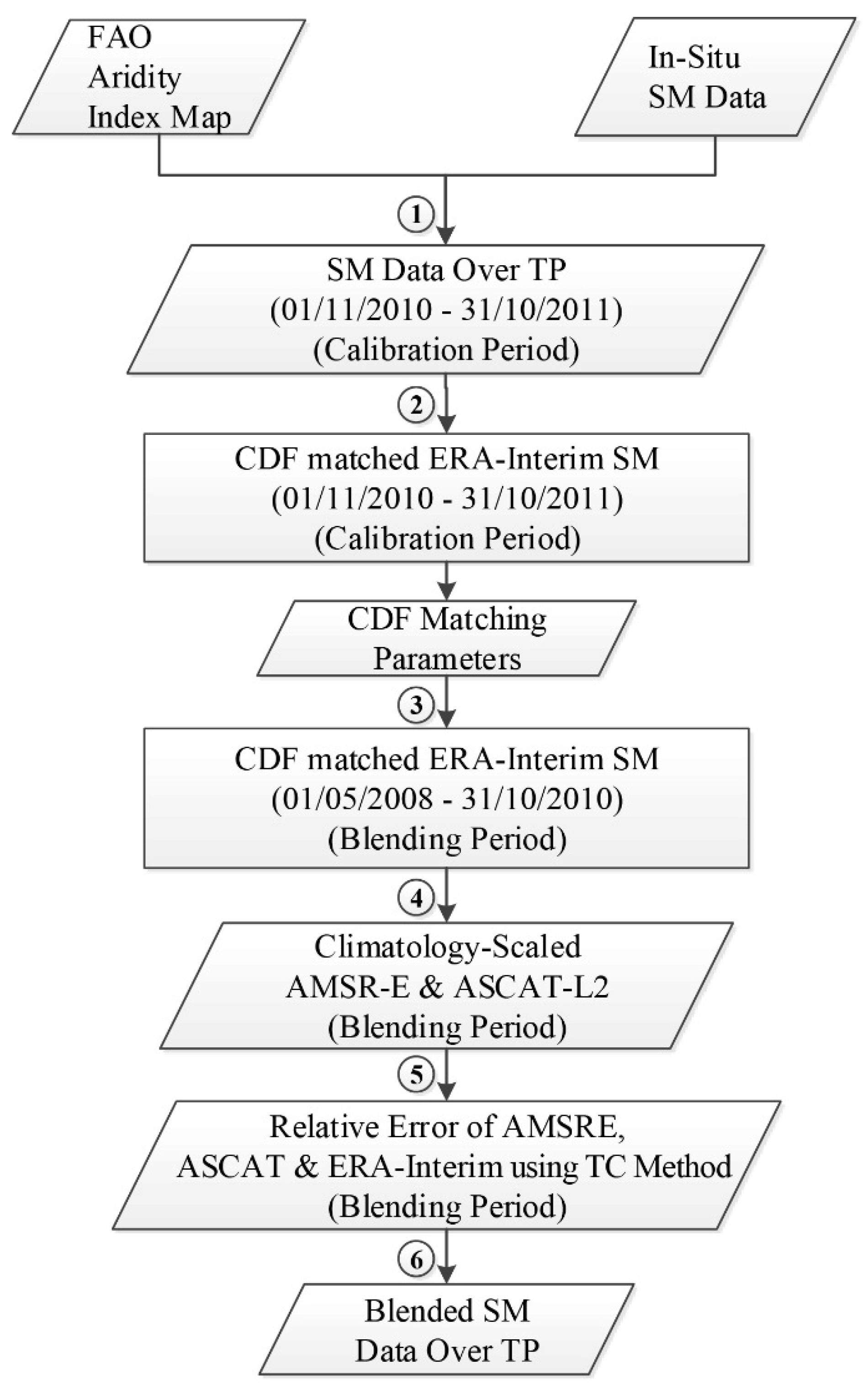
2.2.1. Flowchart

Following the discussion in Section 1.2, we will first use the in situ measurements over TP to limit the data climatology of reanalysis data. The climatology-scaled reanalysis data will be subsequently used as the reference to constrain the climatology of satellite data. The scaled satellite and reanalysis SM data, with consistent data climatology, will be blended to generate a consistent set of SM data over TP.
Herein lies two major challenges: (1) the short record of in situ observed SM data has to be used under the constraint that we do not have global estimates of the temporal statistical moments; (2) the SM data over the sparsely distributed in situ networks has to be used under the constraint that global estimates of the spatial statistical moments of the data over TP is unknown.
To tackle the first challenge, we will use the in situ SM for 12 months (1 November 2010–31 October 2011, calibration period) to determine scaling parameters for the reanalysis data. The ERA-Interim SM product will be adopted as the reanalysis data for this study [12]. The 12-month in situ data is deemed appropriate to capture the seasonal statistical moments, by using CDF matching technique [39,42].
These scaling parameters are then applied to the ERA-Interim SM data during the period 1 May 2008–31 October 2010 (blending period). The selection of the calibration and blending periods is limited by the in situ data availability. Before May 2008, only thebNaqu network was equipped with five observation stations. After that, 20 more stations were installed in the Maqu network. It was not until August 2010 both Ali and Shiquanhe networks were equipped with an extra 20 stations, which leads to the Tibet-Obs crossing over three different typical climate conditions over TP [11]. See Figure 1a for geophysical locations of different networks.
To address the second challenge, we will use the FAO Aridity Index map [56,57]. The Aridity Index (AI) is expressed as a generalized expression of precipitation, temperature, and potential evapotranspiration (PET), to quantify precipitation availability concerning the atmospheric water demand [58,59]. The global AI dataset was compared to the USGS (U.S. Geological Survey) Land Characteristics Database [60], and the MODIS (Moderate Resolution Imaging Spectroradiometer) Tree Cover Percentage [61] estimates, to obtain AI thresholds for classifying different climatic zones.
Based on the classification scheme, the TP has been categorized into three climatic zones: arid zone (0.03 < AI < 0.2), semi-arid zone (0.2 < AI < 0.5) and sub-humid zone (0.5 < AI < 1.0) (Figure 1a). The Tibet-Obs networks are distributed throughout the three climatic zones: Ali and Ngari-Shiquanhe networks in the arid zone, Naqu network in the semi-arid zone, and Maqu network in the sub-humid zone. The averaged SM fields of each network are assumed to be representative for the climatic zone in which that network is located. For the arid zone, the averaged SM data over both the Ali and Shiquanhe networks are used.
Figure 3 shows the flowchart on how the scaling and blending were carried out:
(1)
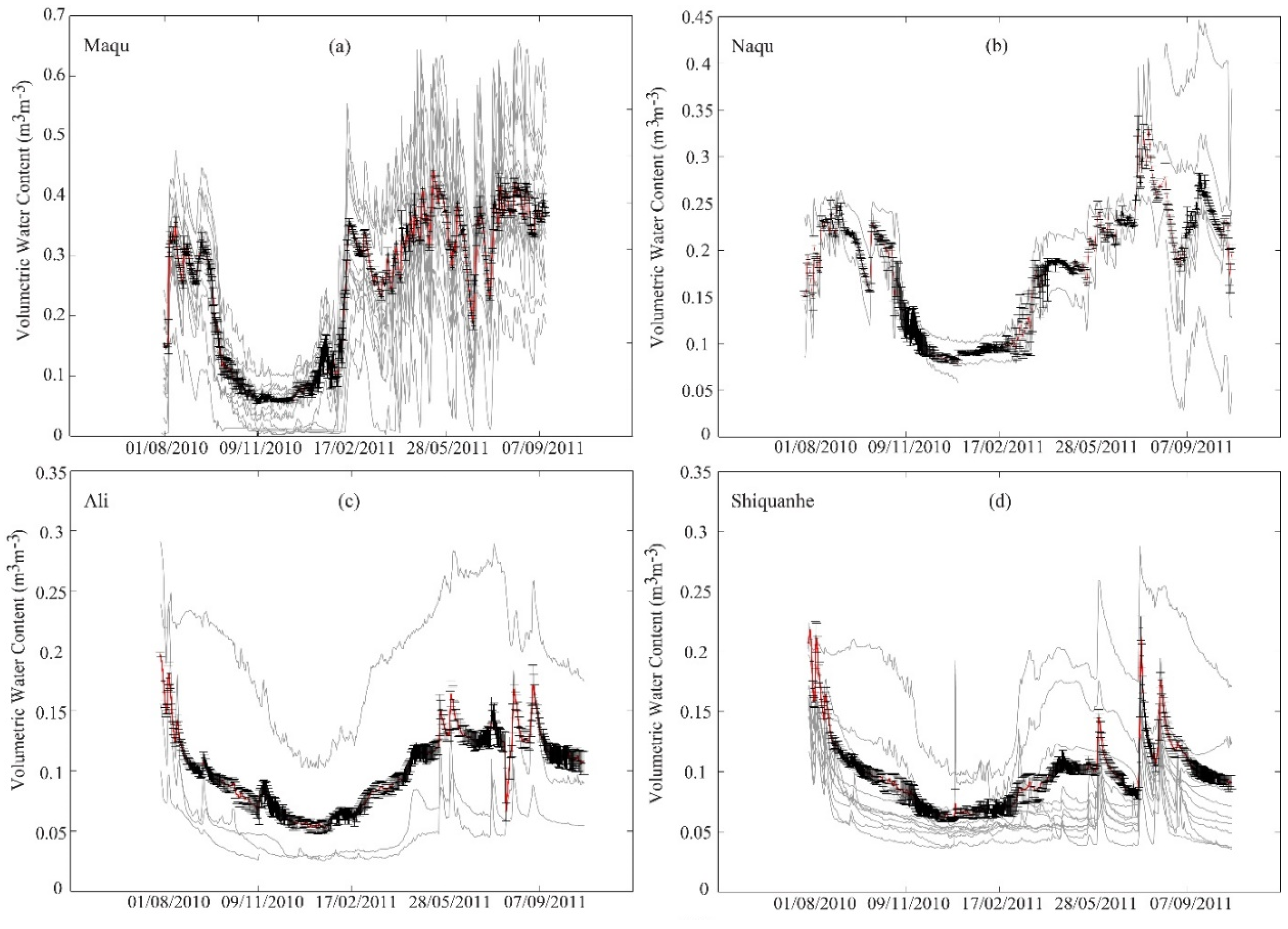
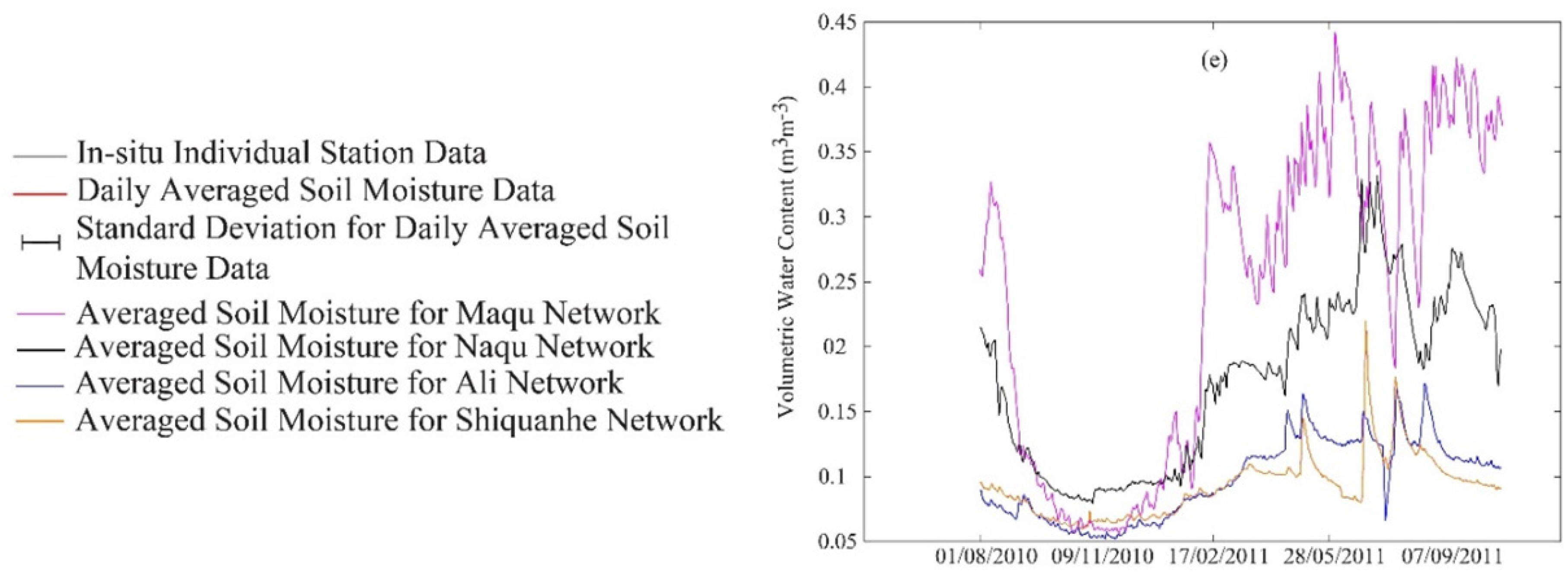
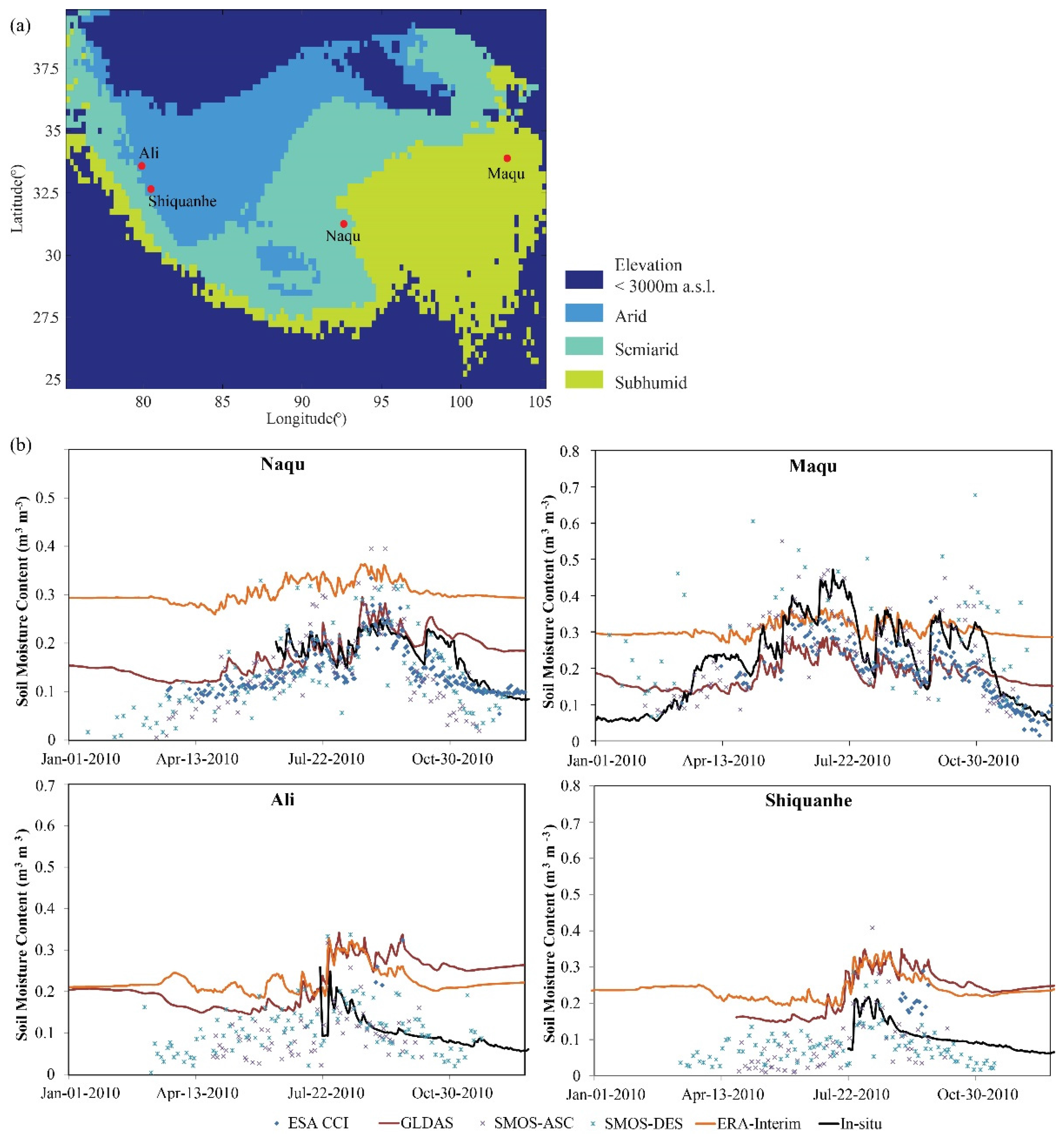
The first step is to generate the 0.25° spatial resolution in situ SM data climatology over TP. The FAO Aridity Index map, combined with in situ measurement, is used to produce in situ SM data climatology over TP, under the assumption mentioned above. For instance, the averaged SM value of both Ali and Shiquanhe is taken as be representative for the arid zone, Naqu for the semi-arid zone, and Maqu for the sub-humid zone (Figure 1a);
(2)
The second step is to generate the scaled ERA-Interim SM data (0.25°) over the calibration period and the associated CDF matching parameters to capture the climatology of the in situ data. The CDF matching parameters will be used in the blending period;
(3)
The third step is to generate the scaled ERA-Interim SM data (0.25°) over the blending period using the CDF matching parameters derived from Step (2);
(4)
The fourth step is to produce the scaled AMSRE and ASCAT SM data (0.25°), with the scaled ERA-Interim SM data generated from Step (3);
(5)
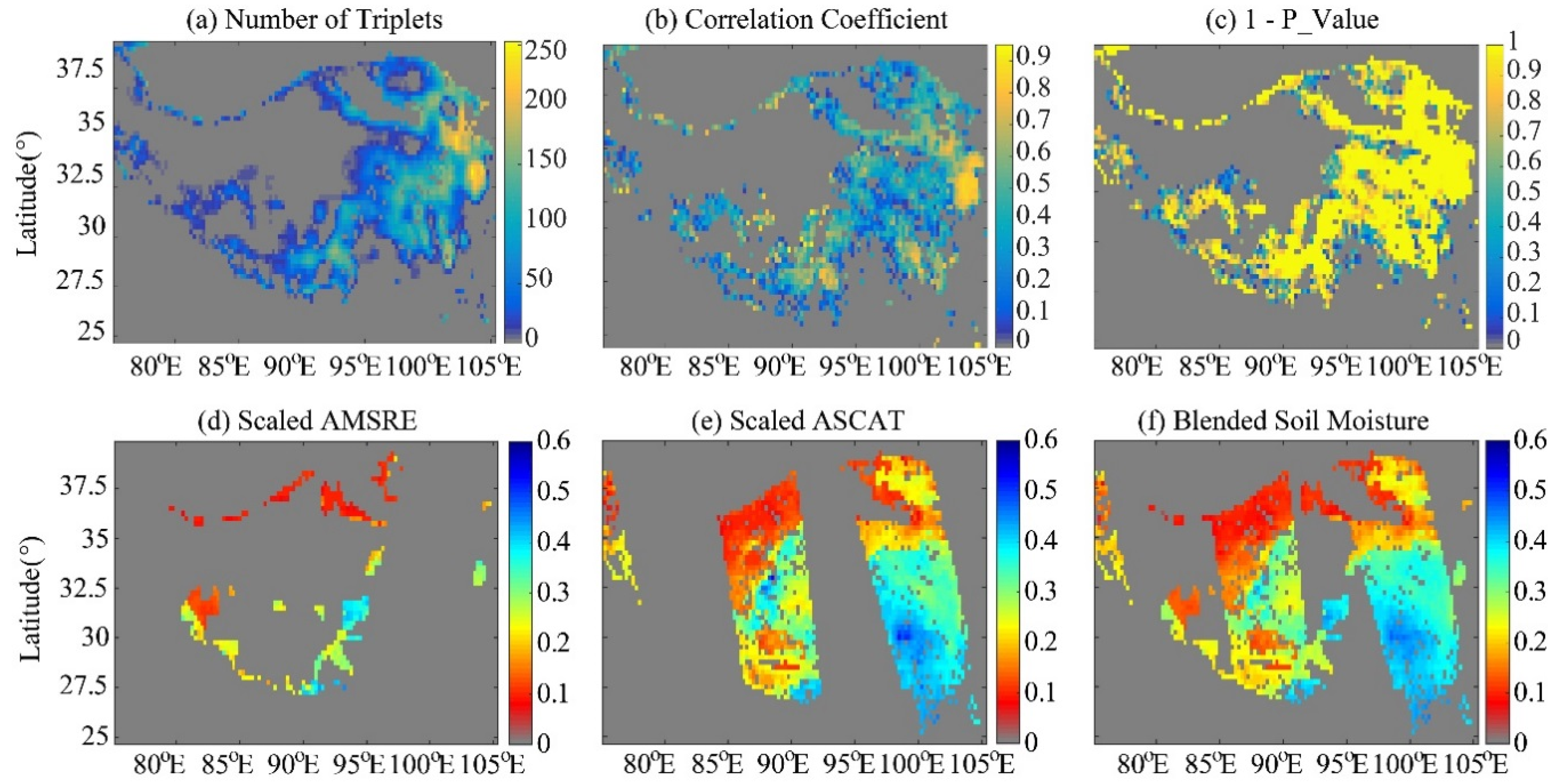
The fifth step is to determine the relative errors among the three scaled SM data sets (i.e., AMSRE, ASCAT, and ERA-Interim), by using the Triple Collocation (TC) method;
(6)
The sixth step, the scaled AMSRE, ASCAT, and ERA-Interim SM data are blended using the least squares method.

2.2.2. CDF Matching

CDF matching technique has been widely used for bias reduction in satellite-retrieved surface SM [32,39,41,42,62]. Technically, the reference in situ SM data and the to-be-scaled SM data (model-simulated/satellite-observed) have to be ranked. Consecutively, the differences between the corresponding elements of each ranked dataset have to be calculated, which are subsequently plotted against the satellite data. Then, a piece-wise linear CDF matching technique is used to derive the bias-corrected SM datasets [25,32]. The piece-wise linear CDF matching approach divides the CDF curve into a certain number of segments, performs linear regression analysis for each segment, and uses the linear equations (slope and intercept) to scale data falling into different segments.

2.2.3. Objective Blending

Yilmaz et al. [63] introduced an objective methodology for blending satellite- and model-based SM products in the least squares framework where uncertainty estimates for each product are obtained using the TC method. This study will adopt the same methodology to blend the satellite and reanalysis SM data mentioned in Section 2.1.
Least squares is an estimation theory and can be used to describe the basis of most modern data assimilation techniques [64]. The desired estimate of SM, via blending different sources of data using least squares framework, can be expressed as below:
S M b l e n d = ω A M S R E S M A M S R E + ω A S C A T S M A S C A T + ω E R A I n t e r i m S M E R A I n t e r i m
where ω A M S R E , ω A S C A T , and ω E R A I n t e r i m are the relative weights of the AMSRE, ASCAT. and ERA-Interim SM products, respectively. To have an unbiased optimal merged estimation, it is required that ω A M S R E + ω A S C A T + ω E R A I n t e r i m = 1 . The relative weights of different SM products are expressed as:
ω A M S R E = σ A S C A T 2 σ E R A I n t e r i m 2 σ A M S R E 2 σ A S C A T 2 + σ A M S R E 2 σ E R A I n t e r i m 2 + σ A S C A T 2 σ E R A I n t e r i m 2 ω A S C A T = σ A M S R E 2 σ E R A I n t e r i m 2 σ A M S R E 2 σ A S C A T 2 + σ A M S R E 2 σ E R A I n t e r i m 2 + σ A S C A T 2 σ E R A I n t e r i m 2 ω E R A I n t e r i m = σ A M S R E 2 σ A S C A T 2 σ A M S R E 2 σ A S C A T 2 + σ A M S R E 2 σ E R A I n t e r i m 2 + σ A S C A T 2 σ E R A I n t e r i m 2
where σ AMSRE 2 , σ ASCAT 2 , and σ ERA Interim 2 are the variance of AMSRE, ASCAT, and ERA-Interim SM products, respectively. If only two SM estimations available, the least square method can be applied similar, with weights:
ω P r o d 1 = σ P r o d 2 2 σ P r o d 1 2 + σ P r o d 2 2 ;   ω P r o d 2 = σ P r o d 1 2 σ P r o d 1 2 + σ P r o d 2 2
It is to be noted that the error variance in Equation (2) should not be regarded as the absolute values of the error variances, but the relative accuracy of the three sets of SM products (e.g., three independent realizations of true SM states) [63], which can be determined by using the TC method. The relative accuracy of these realizations represents how the noisiness of one product compares against that of another product. The TC method has been developed to use three collocated datasets for jointly providing sufficient constraints determining the relative error variance to characterize the uncertainties [65]. It can help to identify individual relative error structure of in situ, remote sensing, and reanalysis datasets. For the detailed description of TC method, readers are referred to Vogelzang and Stoffelen [66] and Yilmaz et al. [63]. When there are only two SM products, the variances of the two available products will be used to derive, deterministically, the weight coefficients according to Equation (3).

3. Results

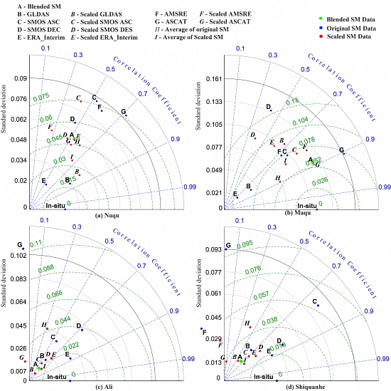
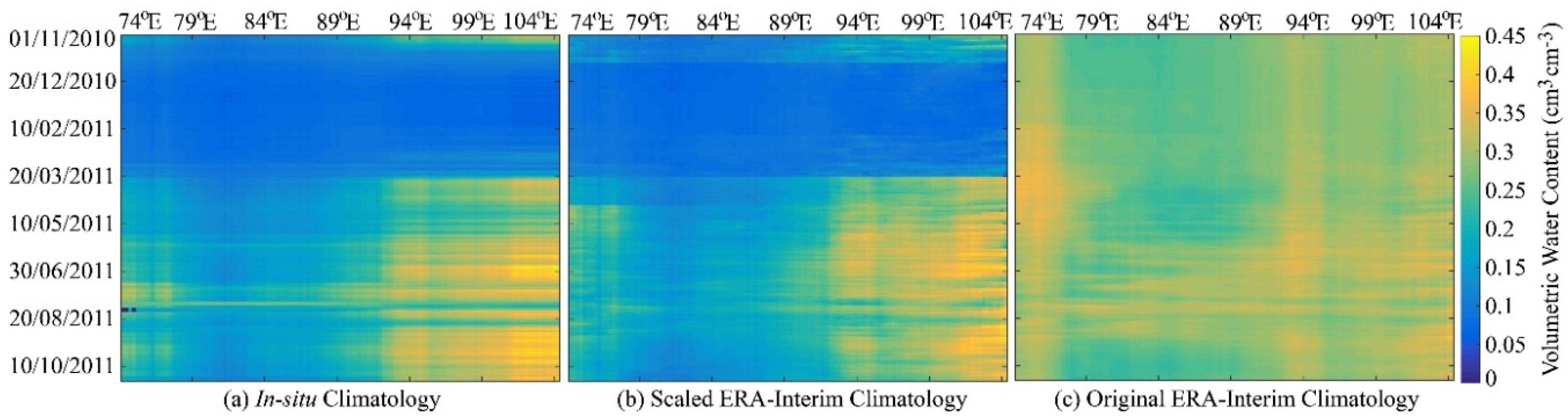
3.1. Calibration Results

As indicated in Section 2.2.1, the original ERA-Interim SM data will be scaled to the in situ data climatology, which was generated by the combined use of the in situ observation (Figure 2) and the FAO aridity index map (Figure 1a), for the calibration period between 1 November 2010 and 31 October 2011. This process involves the first two steps as indicated in the flowchart of scaling and blending (Figure 3).
We used time-longitude diagrams to investigate the calibration results. The time-longitude diagram shows the temporal evolution of the zonal average (e.g., latitude-wise) of SM data along the longitude across the TP. Figure 4 displays the time-longitude diagram for the original ERA-Interim and the scaled ERA-Interim SM products, based on in situ climatology.
The original ERA-Interim SM product (Figure 4c) shows a relatively smoother SM variation over the TP than the in situ climatology (Figure 4a). This “smoothness” pattern of ERA-Interim data is corresponding to the earlier reported results [12]. After being scaled by using the CDF matching method, the scaled ERA-Interim product (Figure 4b) shows a similar pattern to the time-longitude diagram of in situ climatology.
For example, the eastern TP (e.g., 94°E–104°E) is relatively dry with zonal averaged SM of 0.05–0.1 cm3·cm−3 during the winter season (e.g., 1 November 2010–20 March 2011), while it is relatively wet (0.35–0.45 cm3·cm−3) during the monsoon season (e.g., 10 May 2011–10 October 2011) (Figure 4a,b). However, such seasonal change of the eastern TP can be only weakly found in the original ERA-Interim climatology (Figure 4c). Additionally, Figure 4a,b show that the western TP (e.g., 74°E–89°E) is drier than the eastern TP, which is again only weakly and partially represented by the non-scaled ERA-Interim SM product.
The ERA-Interim SM product was scaled to the in situ climatology, based on different seasons across the calibration period. The calibration period was divided into four seasonal categories [67]: the winter season (December–March), the transition 1 (April) from winter to the monsoon, the monsoon season (May–October), and the transition 2 (November) from monsoon to winter. The scaling parameters for these four seasonal categories will be used to generate the scaled ERA-Interim SM product over the blending period between 1 May 2008 and 31 October 2010. This approach is following Reichle and Koster [39], who applied the scaling parameters, generated from one year of the SMMR (Scanning Multichannel Microwave Radiometer) SM record to the nine years of SMMR data.

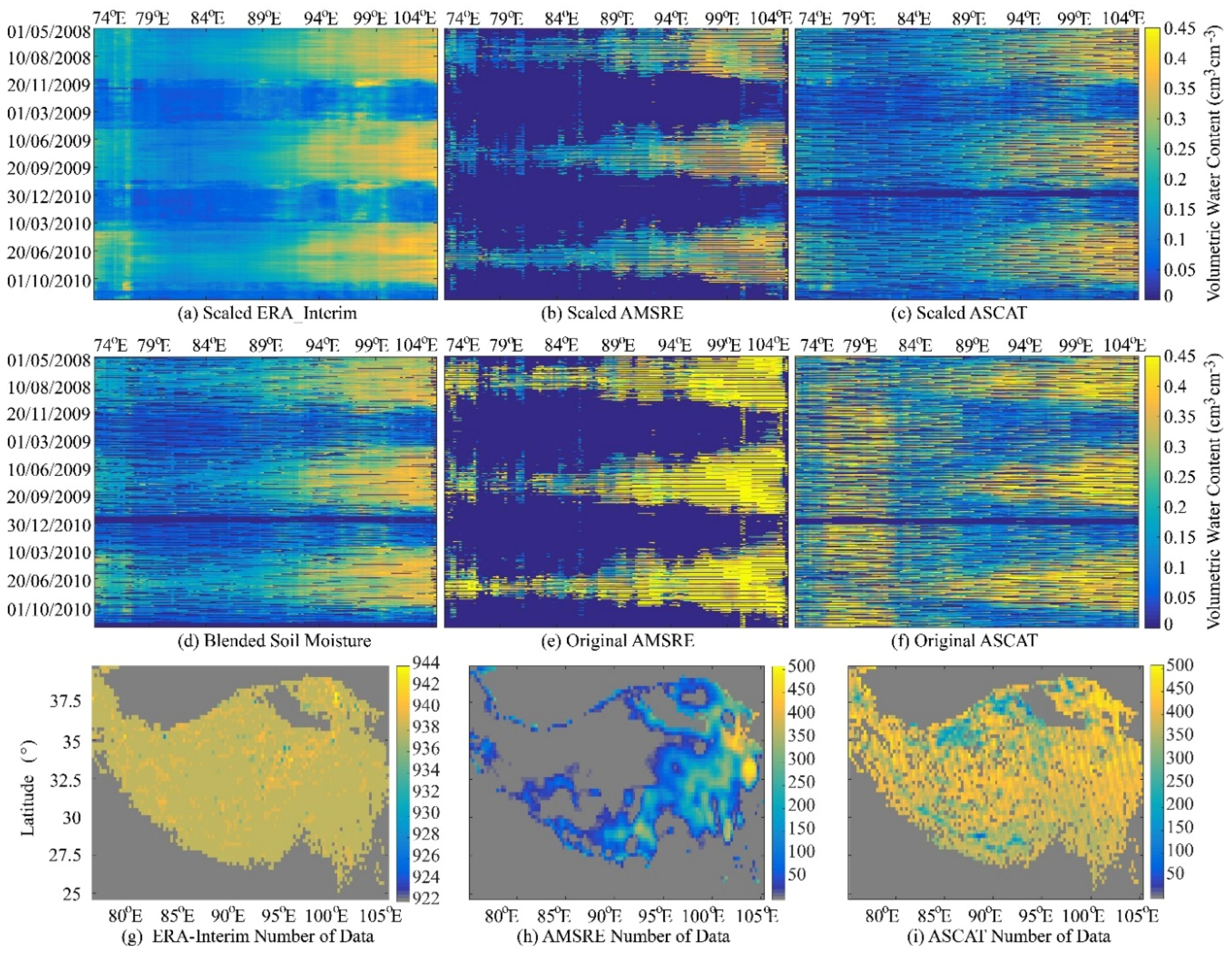
3.2. Blending Results

This sub-section will present the scaled ERA-Interim and satellite SM products (i.e., Step 3 and 4 in Figure 3) and the blended SM data (i.e., step 5 and 6 in Figure 3), for the blending period. Figure 5 shows that the scaled AMSRE (Figure 5b) and ASCAT (Figure 5c) SM products have the similar spatial and temporal patterns of soil wetness over the TP, when compared with the scaled ERA-Interim SM data (Figure 5a). All three scaled SM products show the seasonal variation of SM over the eastern TP, and represent the relatively dry western TP.
Figure 5e,f show the time-longitude diagram for the original satellite SM products. Although both original AMSRE and ASCAT products capture roughly the spatiotemporal pattern, both products are overestimating the SM over the TP. This overestimation is especially evident for AMSRE data. The dark blue area in Figure 5b,e indicates AMSRE observation were flagged out. Compared to AMSRE data, the original ASCAT data can represent more realistic the spatiotemporal SM pattern over TP, except for the unrealistic overestimation over the western TP. Nevertheless, after scaling, both AMSRE and ASCAT data have the similar climatology with the scaled ERA-Interim data.
With the consistent climatology, the scaled AMSRE, ASCAT, and ERA-Interim SM products were blended into one set of SM data, using the objective blending method introduced in Section 2.2.3. Figure 5d shows that the spatiotemporal pattern of the blended SM is close to that in Figure 5a. The blending of the three scaled SM products was implemented with two sub-steps: (i) blending the three collocated SM data (see Figure 6a–c); (ii) blending the rest of data, which means the two satellite SM data collocate individually with the scaled ERA-Interim data, but not collocating with each other (see Figure 6d,e).
The collocated SM data among the three SM datasets over the blending period were identified in Figure 6a. It shows that the triplet numbers greater than 100 were mainly distributed over the eastern TP and partially over the southern TP. When more than 100 data points collocating with each other between the three scaled SM products, the number of the triplet is then equal to 100. It is advised that at least 100 observation triplets are required for a reliable estimation of the relative error among the three SM products. Below 100 observations the limited sample size can lead to systematic effects of up to 5% [68].
To check if the identified number of triplets is statistically significant to be applied with TC method, the minimum correlation coefficient (hereafter as CC) among the three collocated SM products is calculated. Figure 6b shows that the minimum CCs with a value >0.15 (e.g., required for statistical significance at the 5% level for the sample size of 100) were corresponding to those regions with triplet number >100. Figure 6c shows the significance level of the minimum CC over the TP and indicates that the area with triplet number >100 are all statistically significant (e.g., p-value < 0.05) to be applied with TC method to identify the relative error. It is to be noted that the Figure 6c was plotted with (1−p-value). This was done to make the plot visible with p-values, most of which were close to zero. The identified relative errors are then used as inputs for the least squares method to blend the three scaled SM products, according to Equation (2).
The second sub-step is to blend the scaled satellite SM data collocating individually with the scaled ERA-Interim data, but not collocating with each other by themselves (Figure 6d,e). The weights for blending between the scaled AMSRE and ERA-Interim, or the scaled ASCAT and ERA-Interim, were determined by using Equation (3). As can be seen from Figure 6d–f, both the scaled AMSRE and ASCAT were blended into the final SM product.

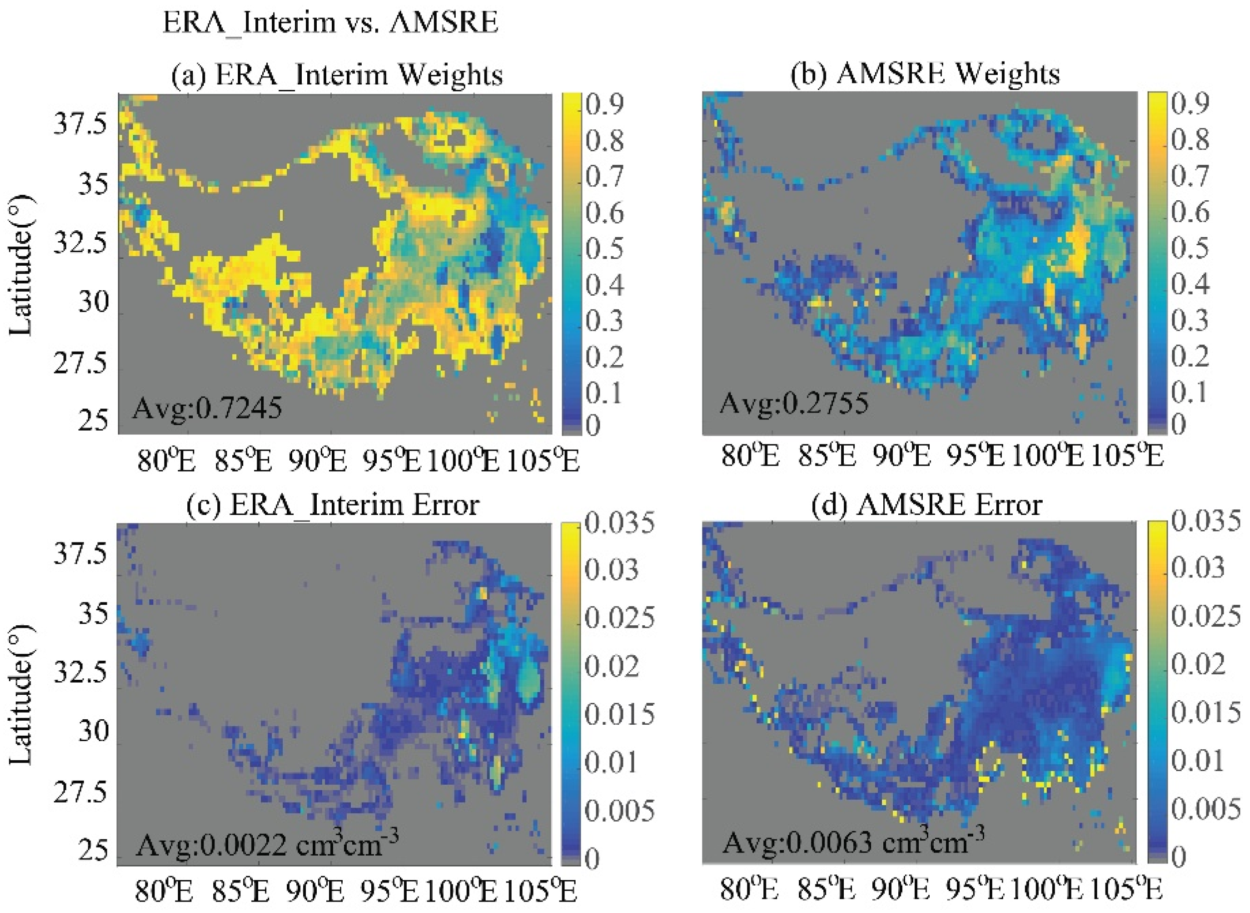
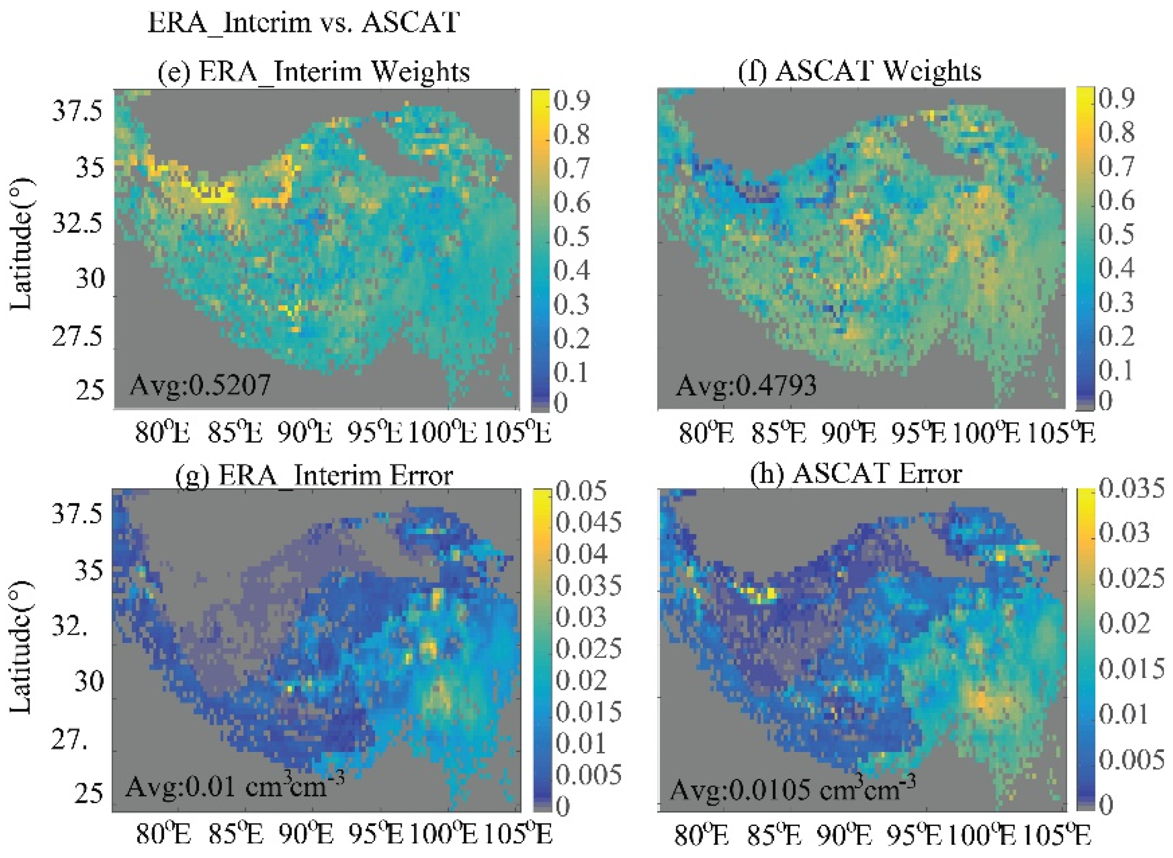
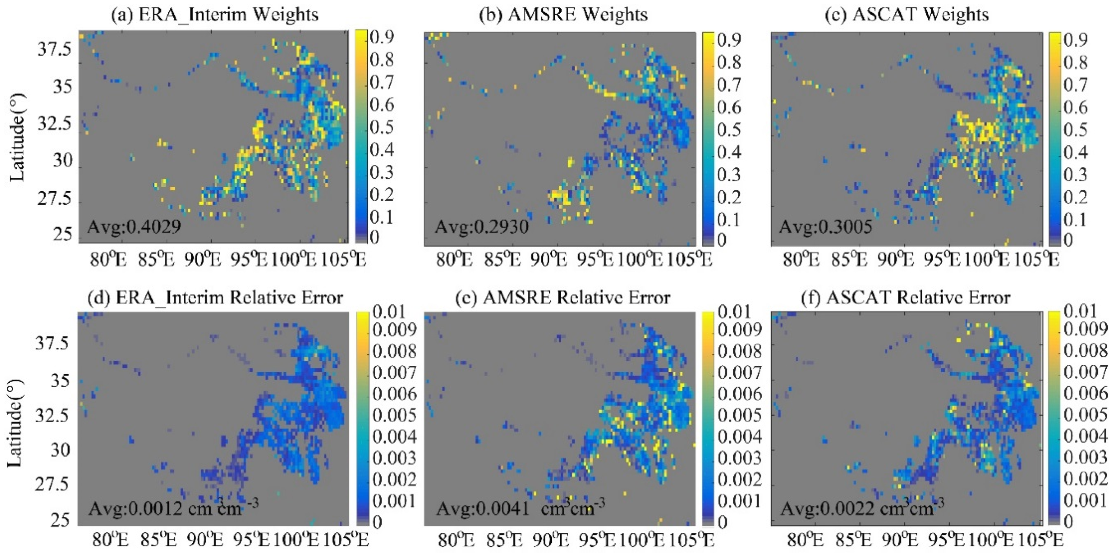
3.3. Weights and Relative Errors

Figure 7 shows the weights and relative errors of scaled ERA-Interim, AMSRE and ASCAT, determined by least squares and TC, for the blended SM. It was as expected that the weights and relative errors were mainly calculated over the eastern TP, where the collocated observations concentrated (Figure 6). Among the three scaled SM products, the ERA-Interim has the smallest average relative error (0.0012 cm3·cm−3) while the greatest weight (0.4029) contributing to the blended SM. There are no significant differences in average weights between AMSRE (0.2930) and ASCAT (0.3005), indicating almost the same contribution to the blended SM over the TP. A closer look at the geographical distribution of higher weights (>0.9, yellowish parts in Figure 6a–c), the scaled AMSRE seems more reliable (i.e., higher weights while lower relative errors) over the southern TP (sparsely vegetated/semi-arid), while the scaled ASCAT more reliable over the eastern TP (moderate vegetated/sub-humid).
Figure 8 shows the weights and relative errors for those scaled AMSRE and ASCAT data, which were not collocating with each other but collocated with the scaled ERA-Interim data. For ERA-Interim vs. AMSRE results, the average weight of ERA-Interim is 0.7245, and the average weight of the scaled AMSRE is 0.2755 (Figure 8a,b), corresponding with a relative error of 0.0022 cm3·cm−3 and 0.0063 cm3·cm−3, respectively. Figure 8a shows the weights with a value of >0.9 for ERA-Interim were mainly distributed over the central and western TP, while only a small portion of the eastern TP had a weight value of >0.9 for the scaled AMSRE (Figure 8b). This sparseness of AMSRE was mainly due to the small SM retrieval rate of AMSRE over the central and western TP, where the permafrost and seasonally-frozen ground were widespread (see Figure 5h). Such a limitation was inherent to microwave theory, in regards to distinguishing if the soil is getting dry or frozen [13,14]. The current solution to this difficulty is to have advisory flags for frozen soil, which leads immediately to the low SM retrieval rate of AMSRE.
For ERA-Interim vs. ASCAT results, the average weight of ERA-Interim (0.5207) is very close to that of the scaled ASCAT (0.4793), as well as for the relative errors (0.01 cm3·cm−3 and 0.0105 cm3·cm−3, respectively). Although the original ASCAT SM product can be noisy and not reliable over the cold semi-arid and arid regions on the TP (results not shown), the scaled ASCAT data are within the range of SM variation (see Section 3.5). It shares almost the same weight as the ERA-Interim concerning the contribution to the blended SM (Figure 8e,f).

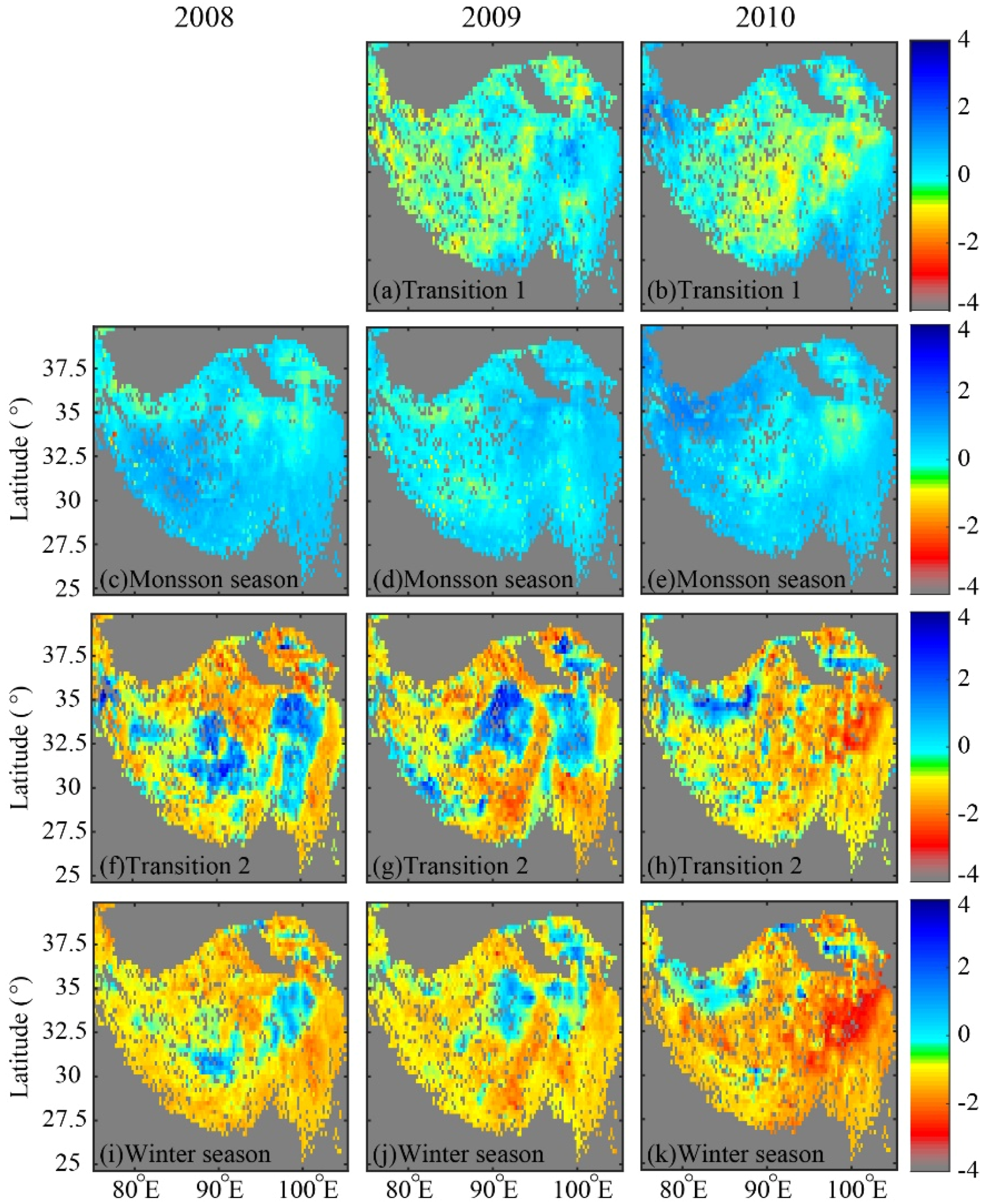
3.4. Anomalies of Blended SM

Figure 9 shows how the anomalies of the blended SM product varies seasonally, according to the definition of different seasonal phases mentioned in Section 3.1. The anomalies were calculated considering the blending period as the reference period, following the equation shown as below [69]:
A n o ( i ) = S M ( i ) S M R e f _ P e r i o d ¯ S t d ( S M R e f _ P e r i o d )
where Ano(i) is an anomaly of the blended SM estimate ( S M ( i ) ) at day i, while S M R e f _ P e r i o d ¯ and S t d ( S M R e f _ P e r i o d ) are the averaged SM value and the standard deviation (hereafter as Stdev), respectively. The anomaly is normalized to the Stdev and is dimensionless.
During the Transition 1 period, the SM anomalies become positive, starting from the eastern and southern part of the TP, especially for 2009 (Figure 9a). While, for 2010, the positive anomalies can also be seen from marginal areas of the TP (Figure 9b). This positive anomaly, perhaps, corresponds to the wetter summer monsoon in 2010 than in 2009, as indicated by the Indian monsoon index [70]. The positive anomalies spread over the whole TP during the monsoon season (Figure 9c–e) for the blending period between 1 May 2008 and 31 October 2010.
After that, the TP starts the drying process (with negative SM anomalies) throughout the transition two period and the winter period. From the drying pattern during the transition two period in 2008 and 2009, it seems the drying starts from the northern and southern TP, and then to the central TP (Figure 9f,g). While, for 2010, the drying is much stronger over the eastern TP than other regions (Figure 9h). In general, the drying in 2010 is more substantial than that in 2008 and 2009, which can be seen from Figure 9i–k as well. It is noticed that the SM over the central TP (ca. 31°N, 90°E) in 2008 and 2009 are not decreasing during the winter period. The SM anomalies over the central TP are close to zero or even positive (Figure 9i–k). This SM anomaly may contribute to the recently-identified increasing trend of SM over the central TP [71,72]. While, in 2010, such a zone of positive anomalies was pushed from the central TP to the northwestern TP.

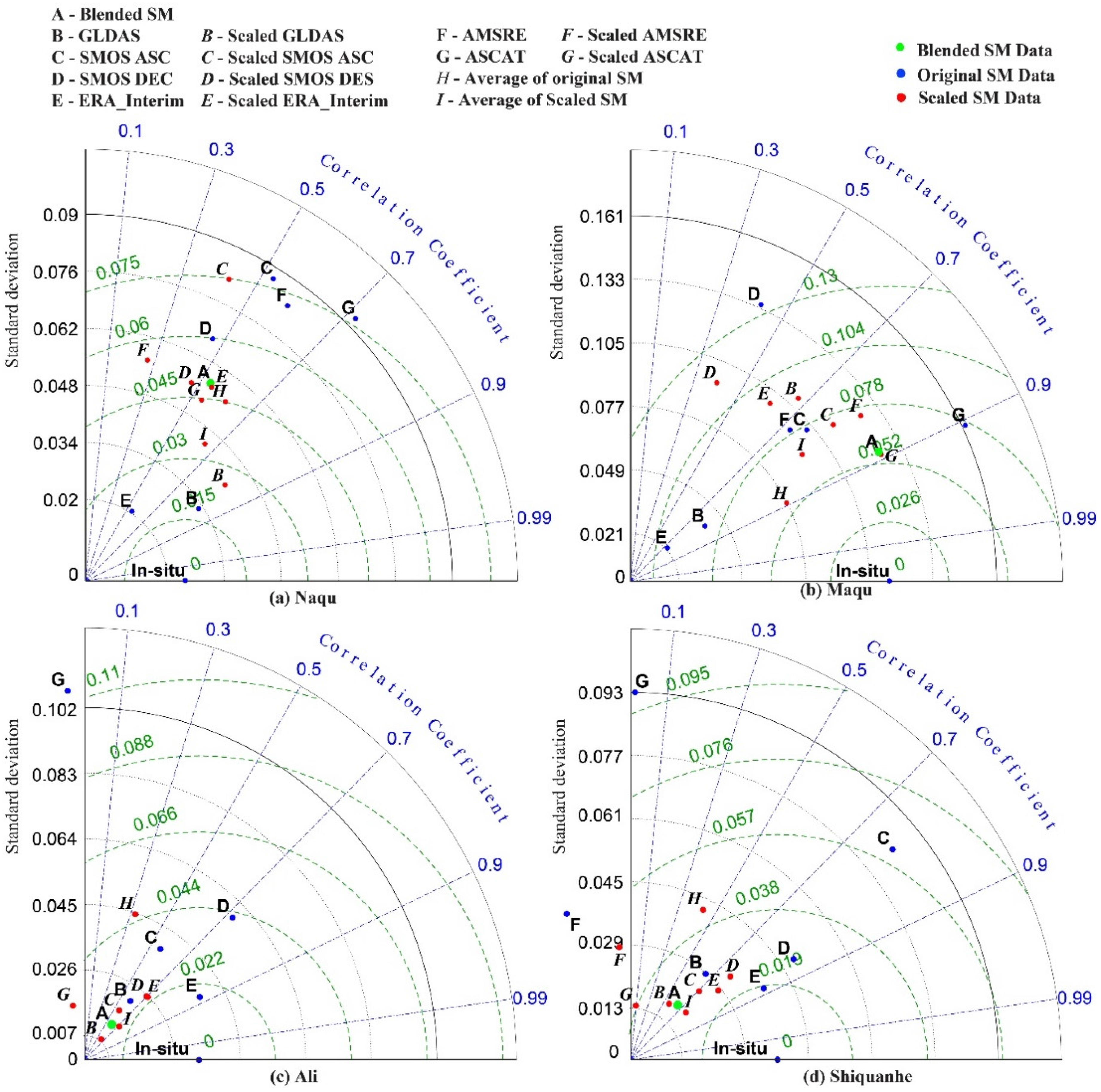
3.5. Inter-Comparison

In this section, the blended SM was compared with different SM products for the period between 1 January 2010 and 31 October 2010, against with the in situ measurements over Tibet-Obs networks (Naqu, Maqu, Ali, and Shiquanhe). The SM products include AMSRE, ASCAT, SMOS ascending and descending data, GLDAS, ERA-Interim, and their corresponding scaled SM data. Additionally, the equal weighting average of multisource original SM data and their scaled SM data were also inter-compared in Figure 10.
Without being scaled to the climatology constrained by in situ data, the AMSRE and ASCAT SM data (F and G in Figure 10) have larger Stdevs (standard deviation) than the measurements. This larger Stdevs indicates that their variability is greater than that of the in situ measurements. After scaling, the variation range of both scaled AMSRE and ASCAT data (F and G in Figure 10) are brought closer to that of in situ observation. For example, at Naqu network, the Stdevs of F and G are 0.084 and 0.092 cm3·cm−3, and after scaling, the Stdevs of F and G are 0.056 and 0.053 cm3·cm−3, which are much closer to the Stdev of the in situ data (0.024 cm3·cm−3). Such an effect of scaling can also be seen in Figure 5 at the plateau scale.
From Figure 10a–d, one can also see that the scaled ASCAT (G) is much closer to the blended SM data (A) than the scaled AMSRE data (F). This closeness shows that the scaled ASCAT SM data accounts for a bigger weight than the scaled AMSRE data in the blended SM. It is to be noted that for the Ali and Shiquanhe networks over arid regions, both the original and scaled AMSRE and ASCAT SM data cannot capture the in situ measured SM dynamics. All four points are on the lines of correlation coefficient being close to zero or being negative. On the contrary, the scaled SMOS ASC and DEC SM data (C and D in Figure 10) can capture quite well the SM dynamics over Ali and Shiquanhe networks, and perform similarly as the blended SM does. Across the TP, the scaled SMOS SM data perform better under arid conditions (C and D in Figure 10c,d) than under semi-arid and sub-humid conditions (C and D in Figure 10a,b).
At the Maqu network, under the sub-humid environment, the blended SM shows a match with the in situ data concerning the variability, but underestimates the observation, especially during the monsoon period (time series resulst not shown). On the contrary, the original ERA-Interim data overestimates the observation during the winter period and underestimates it during the monsoon period, which may be induced by the treatment of freezing-thawing process in the land surface scheme used [12,73,74]. The original GLDAS data underestimates the observation almost throughout the whole year, except for during January and December. This underestimation can be seen from B (original GLADA) and E (original ERA-Interim) in Figure 10b, where the Stdevs of both B and E are much smaller than the in situ measurement. At the Naqu network (Figure 10a), other than the original GLDAS (B) and ERA-Interim (E) data, most of SM data have much larger Stdevs than the in situ data. Over the arid regions, at the Ali and Shiquanhe networks (Figure 10c,d), the blended SM (A) keeps relatively stable in a range of 0.05–0.2 m3·m−3.
The equal weighting average of multisource original SM data (H in Figure 10) was underestimating in situ observations in the Maqu network while overestimating in other networks. The equal weighting average of scaled SM data (I in Figure 10) was not performing similarly with the blended SM (A) at sub-humid and semi-arid networks (Figure 10a,b), but at arid networks over Ali and Shiquanhe (Figure 10c,d). The performance of equal weighting averages indicates that the least square weighting approach deployed in this study (see Section 2) is necessary for the central and eastern TP (e.g., cold sub-humid and semi-arid regions), while not necessary for the western TP (e.g., cold arid regions).

4. Conclusions

4.1. Controlling Factors for SM Blending over TP

The analysis in the previous section shows that the proposed scaling and blending approach has the promising potential of utilizing sparse local in situ networks (Figure 1a) for generating a consistently-blended satellite SM product over TP. The blended SM over TP replicates the SM dynamics across different climatic zones, from sub-humid regions to semi-arid and arid regions. Its performance is, however, determined by three major factors: in situ measurements, satellite observations, and the classification of climatic zones.
The model simulated SM product will affect the blended SM result. However, if the model simulated SM results are not constrained by the in situ data climatology, the blended SM data will have different climatology when different models used, which cannot capture the in situ observed SM dynamics (Figure 1b). This highlights, on one hand, the use of in situ data, constraining the model-simulated SM results, can partially ensure that the in situ measured climatology is used as the base for scaling; on the other hand, the further development of model physics (e.g., freezing-thawing process considering vapor transport) [12,75,76,77] should be investigated towards a consistent representation of the physical processes in LSMs over the TP.
On the other hand, the quality of satellite data plays another crucial role in producing a sound, blended SM product. When the satellite SM data shows certain correlation with the in situ data, the blended SM can correct its systematic bias as showed in Figure 5. The Figure 10c,d show that the lack of good quality satellite data leads to a poor performance of the blended SM product, even though the blended SM product has the improved statistic scores compared to that of the original satellite data.
By the nature of the scaling and blending strategy (Section 2.2), it is anticipated that different climate classification schemes will result in different SM products [78]. The climate classification used in this study is based on the aridity index [59], which is expressed as a generalized expression of precipitation, temperature, and potential evapotranspiration (PET), to quantify precipitation availability over atmospheric water demand. It is also expected that different calculation schemes for the aridity index will alter the blended SM product [79,80]. However, a detailed examination of the effect of various schemes of climate classification and aridity index on the blended SM product is beyond the objectives of this paper. As discussed, this study tries to demonstrate if we can generate a consistently-blended satellite SM data, constrained by the observed in situ climatology.

4.2. Brief Summary

In this study, the in situ SM measurement from the Tibet-Obs is used to scale the model-simulated SM climatology of ERA-Interim. With the utilization of the FAO aridity index map, the TP is classified into sub-humid, semi-arid, and arid climatic zones. There are three regional-scale networks operated accordingly in these three classified climatic zones. It is assumed that SM climatology measured by each network is representative for the SM climatology of the climatic zone, where this network is located. As such, the in situ SM climatology over the TP is produced to scale ERA-Interim SM data. Subsequently, the climatology-scaled ERA-Interim SM product is deployed as the reference to scale satellite observed SM products. By using the TC and the least squares method, the scaled AMSRE, ASCAT, and ERA-Interim SM products are blended to generate a consistent set of SM products for the whole TP (Figure 6).
The results show that the scaling and blending strategy help constraining the exaggerated variation of satellite SM over the TP, especially the unrealistically high SM content over the western TP. The unrealistic high SM over the west TP persists throughout the whole year and can be even higher in the winter period than in monsoon period. This is mainly due to the overestimation of AMSRE data over semi-arid and arid regions in the winter period as reported in [11,12]. It is, however, to be noted that the availability of AMSRE data over the plateau is little, especially during winter periods. After implementing the scaling and the blending steps (Figure 3), the overestimation was eliminated in the blended SM products (Figure 5), which shows clear seasonal variations and has a good match with the in situ measurements (Figure 10).
The inter-comparison results indicated that an equal weighting average of multi-sources of scaled SM data can perform similarly as the blended SM data over the cold arid regions, but not over the cold sub-humid areas on the TP (see I in Figure 10). The simple average of multi-sources of original SM data cannot capture the in situ SM dynamics as the blended SM does (see H in Figure 10). The results suggest that the equal weighting would penalize the contribution from those scaled SM datasets with relative lower noise while falsely enlarging the contribution from those SM datasets with greater noise. Such false enlargement of noise SM data is especially the case for the cold sub-humid areas on the TP (see I and A in Figure 10a).

4.3. Recommendations

As summarized above, this study analyzes the inconsistency among different SM products over the TP and highlights the challenges in generating a consistent SM product over the TP. Such a challenge needs a deeper investigation into the data generation algorithm of each data product (e.g., satellite, in situ, or reanalysis).
From the satellite product viewpoint, these challenges spread from prelaunch calibration, post-launch calibration, on-board calibration, on-ground calibration, and inter-sensor calibration to retrieval algorithms [13,81]. From the in situ measurement perspective, the challenges exist and are not limited to the harmonization of measurement techniques, implementation of in situ networks, sensor calibration, quality control, characterization of representativeness, long-term stability, and reference procedures [13,82,83,84,85]. For the reanalysis products, apart from getting benefit from the improvement of the observation (e.g., both satellite and in situ) in dealing with the challenges as mentioned, the development of model physics and data assimilation schemes will undoubtedly contribute to producing a more consistent SM product [12,86,87,88]. Fortunately, the urgent need for such efforts has been given high and continuous attentions by the scientific and the end-user communities (e.g., space agencies, climate working groups, insurance companies, local governments, etc.). For example, the recently accomplished FP7 project CORE-CLIMAX (http://www.coreclimax.eu/) has made efforts in coordinating earth observation data validation (both satellite and in situ) for reanalysis for climate services.
Last, but not least, the in situ SM and soil temperature measurements are valuable references in this particular environment and shall be maintained and updated whenever possible. The network, Tibet-Obs, used in this study and the one established by Yang et al. [21] possess more than 100 stations on the TP. There are many more SM stations installed by the Third Pole Environment in situ component [22]. These networks provide a representative coverage of the different climate and land surface hydro-meteorological conditions over the TP. The obtained observation data can help to ensure the consistency in classifying the regional climatic conditions and for the purpose of validating or assessing coarse resolution satellite and model-simulated SM products.

Acknowledgements

This work was financially supported in part by the ESA-MOST Dragon III programme, the European Commission CEOP-AEGIS project (Call FP7-ENV-2007-1 Grant No. 212921) (http://www.ceop-aegis.org/), CORE-CLIMAX project (Call SPA.2012.1.3-02 Grant No. 313085), the ESA STSE WACMOS project (www.WACMOS.org), the National Natural Science Foundation of China (41530529), and the Key Research Program of the Chinese Academy of Sciences (KZZD-EW-13). Sincere thanks also go to all other participating colleagues and students for their dedications to these projects and the data collection campaigns.

Author Contributions

Yijian Zeng and Zhongbo Su conceived and designed the research; Yijian Zeng, Lichun Wang and Kai Xu performed the research and analyzed the data; Rogier van der Velde contributed commenting on the primary draft; Jun Wen and Xing Wang contributed maintaining the Tibet-obs networks; Yijian Zeng wrote the paper.

Conflicts of Interest

The authors declare no conflict of interest.

References

  1. Boos, W.R.; Kuang, Z.M. Sensitivity of the South Asian monsoon to elevated and non-elevated heating. Sci. Rep. 2013, 3. [Google Scholar] [CrossRef] [PubMed]
  2. Wu, G.X.; Liu, Y.M.; He, B.; Bao, Q.; Duan, A.M.; Jin, F.F. Thermal controls on the asian summer monsoon. Sci. Rep. 2012, 2. [Google Scholar] [CrossRef] [PubMed]
  3. Yao, Y.H.; Zhang, B.P. A preliminary study of the heating effect of the Tibetan Plateau. PLoS ONE 2013, 8, e68750. [Google Scholar] [CrossRef] [PubMed]
  4. Qiu, J. Monsoon melee. Science 2013, 21, 1400–1401. [Google Scholar] [CrossRef] [PubMed]
  5. Koster, R.D.; Dirmeyer, P.A.; Guo, Z.C.; Bonan, G.; Chan, E.; Cox, P.; Gordon, C.T.; Kanae, S.; Kowalczyk, E.; Lawrence, D.; et al. Regions of strong coupling between soil moisture and precipitation. Science 2004, 305, 1138–1140. [Google Scholar] [CrossRef] [PubMed]
  6. Kerr, Y.H.; Waldteufel, P.; Wigneron, J.P.; Delwart, S.; Cabot, F.; Boutin, J.; Escorihuela, M.J.; Font, J.; Reul, N.; Gruhier, C.; et al. The SMOS mission: New tool for monitoring key elements of the global water cycle. IEEE Proc. 2010, 98, 666–687. [Google Scholar] [CrossRef] [Green Version]
  7. Seneviratne, S.I.; Wilhelm, M.; Stanelle, T.; van den Hurk, B.; Hagemann, S.; Berg, A.; Cheruy, F.; Higgins, M.E.; Meier, A.; Brovkin, V.; et al. Impact of soil moisture-climate feedbacks on CMIP5 projections: First results from the GLACE-CMIP5 experiment. Geophys. Res. Lett. 2013, 40, 5212–5217. [Google Scholar] [CrossRef] [Green Version]
  8. Taylor, C.M.; de Jeu, R.A.M.; Guichard, F.; Harris, P.P.; Dorigo, W.A. Afternoon rain more likely over drier soils. Nature 2012, 489, 423–426. [Google Scholar] [CrossRef] [PubMed] [Green Version]
  9. Jung, M.; Reichstein, M.; Ciais, P.; Seneviratne, S.I.; Sheffield, J.; Goulden, M.L.; Bonan, G.; Cescatti, A.; Chen, J.Q.; de Jeu, R.; et al. Recent decline in the global land evapotranspiration trend due to limited moisture supply. Nature 2010, 467, 951–954. [Google Scholar] [CrossRef] [PubMed]
  10. Hirschi, M.; Seneviratne, S.I.; Alexandrov, V.; Boberg, F.; Boroneant, C.; Christensen, O.B.; Formayer, H.; Orlowsky, B.; Stepanek, P. Observational evidence for soil-moisture impact on hot extremes in southeastern europe. Nat. Geosci. 2011, 4, 17–21. [Google Scholar] [CrossRef]
  11. Su, Z.; Wen, J.; Dente, L.; van der Velde, R.; Wang, L.; Ma, Y.; Yang, K.; Hu, Z. The Tibetan Plateau observatory of plateau scale soil moisture and soil temperature (Tibet-Obs) for quantifying uncertainties in coarse resolution satellite and model products. Hydrol. Earth Syst. Sci. 2011, 15, 2303–2316. [Google Scholar] [CrossRef]
  12. Su, Z.; de Rosnay, P.; Wen, J.; Wang, L.; Zeng, Y. Evaluation of ECMWF’S soil moisture analyses using observations on the Tibetan Plateau. J. Geophys. Res. Atmos. 2013, 118, 5304–5318. [Google Scholar] [CrossRef]
  13. Wagner, W.; Hahn, S.; Kidd, R.; Melzer, T.; Bartalis, Z.; Hasenauer, S.; Figa-Saldana, J.; de Rosnay, P.; Jann, A.; Schneider, S.; et al. The ascat soil moisture product: A review of its specifications, validation results, and emerging applications. Meteorol. Z. 2013, 22, 5–33. [Google Scholar] [CrossRef]
  14. Owe, M.; de Jeu, R.; Holmes, T. Multisensor historical climatology of satellite-derived global land surface moisture. J. Geophys. Res. Earth Surf. 2008, 113. [Google Scholar] [CrossRef] [Green Version]
  15. Njoku, E.G.; Chan, S.K. Vegetation and surface roughness effects on amsr-e land observations. Remote Sens. Environ. 2006, 100, 190–199. [Google Scholar] [CrossRef]
  16. Jackson, T.J.; Le Vine, D.M.; Hsu, A.Y.; Oldak, A.; Starks, P.J.; Swift, C.T.; Isham, J.D.; Haken, M. Soil moisture mapping at regional scales using microwave radiometry: The southern great plains hydrology experiment. IEEE Trans. Geosci. Remote Sens. 1999, 37, 2136–2151. [Google Scholar] [CrossRef]
  17. Entekhabi, D.; Njoku, E.G.; O’Neill, P.E.; Kellogg, K.H.; Crow, W.T.; Edelstein, W.N.; Entin, J.K.; Goodman, S.D.; Jackson, T.J.; Johnson, J.; et al. The soil moisture active passive (SMAP) mission. IEEE Proc. 2010, 98, 704–716. [Google Scholar] [CrossRef]
  18. Rodell, M.; Houser, P.R.; Jambor, U.; Gottschalck, J.; Mitchell, K.; Meng, C.J.; Arsenault, K.; Cosgrove, B.; Radakovich, J.; Bosilovich, M.; et al. The global land data assimilation system. Bull. Am. Meteorol. Soc. 2004, 85, 381–394. [Google Scholar] [CrossRef]
  19. Dee, D.P.; Uppala, S.M.; Simmons, A.J.; Berrisford, P.; Poli, P.; Kobayashi, S.; Andrae, U.; Balmaseda, M.A.; Balsamo, G.; Bauer, P.; et al. The ERA-interim reanalysis: Configuration and performance of the data assimilation system. Q. J. R. Meteorol. Soc. 2011, 137, 553–597. [Google Scholar] [CrossRef]
  20. Balsamo, G.; Albergel, C.; Beljaars, A.; Boussetta, S.; Brun, E.; Cloke, H.; Dee, D.; Dutra, E.; Muñoz-Sabater, J.; Pappenberger, F.; et al. ERA-interim/land: A global land surface reanalysis data set. Hydrol. Earth Syst. Sci. 2015, 19, 389–407. [Google Scholar] [CrossRef]
  21. Yang, K.; Qin, J.; Zhao, L.; Chen, Y.; Tang, W.; Han, M.; Lazhu; Chen, Z.; Lv, N.; Ding, B.; et al. A multi-scale soil moisture and freeze-thaw monitoring network on the third pole. Bull. Am. Meteorol. Soc. 2013, 94, 1907–1916. [Google Scholar] [CrossRef]
  22. Ma, Y.; Kang, S.; Zhu, L.; Xu, B.; Tian, L.; Yao, T. Roof of the world: Tibetan observation and research platform. Bull. Am. Meteorol. Soc. 2008, 89, 1487–1492. [Google Scholar] [CrossRef]
  23. Wagner, W.; Dorigo, W.A.; De Jeu, R.; Fernandez, D.; Benveniste, J.; Haas, E.; Ertl, M. Fusion of active and passive microwave observations to create an essential climate variable data record on soil moisture. ISPRS Ann. Photogramm. Remote Sens. Spat. Inf. Sci. 2012, 25, 315–321. [Google Scholar] [CrossRef]
  24. Albergel, C.; de Rosnay, P.; Gruhier, C.; Munoz-Sabater, J.; Hasenauer, S.; Isaksen, L.; Kerr, Y.; Wagner, W. Evaluation of remotely sensed and modelled soil moisture products using global ground-based in situ observations. Remote Sens. Environ. 2012, 118, 215–226. [Google Scholar] [CrossRef]
  25. Brocca, L.; Hasenauer, S.; Lacava, T.; Melone, F.; Moramarco, T.; Wagner, W.; Dorigo, W.; Matgen, P.; Martinez-Fernandez, J.; Llorens, P.; et al. Soil moisture estimation through ascat and amsr-e sensors: An intercomparison and validation study across Europe. Remote Sens. Environ. 2011, 115, 3390–3408. [Google Scholar] [CrossRef]
  26. Scipal, K.; Holmes, T.; de Jeu, R.; Naeimi, V.; Wagner, W. A possible solution for the problem of estimating the error structure of global soil moisture data sets. Geophys. Res. Lett. 2008, 35. [Google Scholar] [CrossRef] [Green Version]
  27. Dorigo, W.A.; Scipal, K.; Parinussa, R.M.; Liu, Y.Y.; Wagner, W.; de Jeu, R.A.M.; Naeimi, V. Error characterisation of global active and passive microwave soil moisture datasets. Hydrol. Earth Syst. Sci. 2010, 14, 2605–2616. [Google Scholar] [CrossRef] [Green Version]
  28. Chen, Y.; Yang, K.; Qin, J.; Zhao, L.; Tang, W.; Han, M. Evaluation of AMSR-E retrievals and GLDAS simulations against observations of a soil moisture network on the central Tibetan Plateau. J. Geophys. Res. Atmos. 2013, 118, 4466–4475. [Google Scholar] [CrossRef]
  29. Zhao, L.; Yang, K.; Qin, J.; Chen, Y.; Tang, W.; Lu, H.; Yang, Z.-L. The scale-dependence of SMOS soil moisture accuracy and its improvement through land data assimilation in the central Tibetan Plateau. Remote Sens. Environ. 2014, 152, 345–355. [Google Scholar] [CrossRef]
  30. Zeng, J.; Li, Z.; Chen, Q.; Bi, H.; Qiu, J.; Zou, P. Evaluation of remotely sensed and reanalysis soil moisture products over the Tibetan Plateau using in situ observations. Remote Sens. Environ. 2015, 163, 91–110. [Google Scholar] [CrossRef]
  31. Su, Z.; Fernandez, D.; Timmermans, J.; Chen, X.; Hungershoefer, K.; Roebeling, R.; Shroder, M.; Schulz, J.; Stammes, P.; Wang, P.; et al. First results of the earth observation water cycle multi—Mission observation strategy (WACMOS). Int. J. Appl. Earth Observ. Geoinf. 2014, 26, 270–285. [Google Scholar] [CrossRef]
  32. Liu, Y.Y.; Parinussa, R.M.; Dorigo, W.A.; De Jeu, R.A.M.; Wagner, W.; van Dijk, A.; McCabe, M.F.; Evans, J.P. Developing an improved soil moisture dataset by blending passive and active microwave satellite-based retrievals. Hydrol. Earth Syst. Sci. 2011, 15, 425–436. [Google Scholar] [CrossRef] [Green Version]
  33. Dorigo, W.A.; Gruber, A.; De Jeu, R.A.M.; Wagner, W.; Stacke, T.; Loew, A.; Albergel, C.; Brocca, L.; Chung, D.; Parinussa, R.M.; et al. Evaluation of the ESA CCI soil moisture product using ground-based observations. Remote Sens. Environ. 2014, 162, 380–395. [Google Scholar] [CrossRef]
  34. Parinussa, R.; De Jeu, R.; Wagner, W.; Dorigo, W.; Fang, F.; Teng, W.; Liu, Y. [Global climate] soil moisture [in: State of the climate in 2012]. Bull. Am. Meteorol. Soc. 2013, 94, S24–S25. [Google Scholar]
  35. De Jeu, R.; Dorigo, W.; Parinussa, R.; Wagner, W.; Chung, D. Soil moisture, state of the climate in 2011. Bull. Am. Meteorol. Soc. 2012, 93, s30–s34. [Google Scholar]
  36. Guo, D.L.; Wang, H.J. Simulation of permafrost and seasonally frozen ground conditions on the Tibetan Plateau, 1981–2010. J. Geophys. Res. Atmos. 2013, 118, 5216–5230. [Google Scholar] [CrossRef]
  37. Van der Velde, R.; Salama, M.S.; van Helvoirt, M.D.; Su, Z. Decomposition of uncertainties between coarse MM5-noah-simulated and fine ASAR-retrieved soil moisture over central Tibet. J. Hydrometeorol. 2012, 13, 1925–1938. [Google Scholar] [CrossRef]
  38. Koster, R.D.; Guo, Z.C.; Yang, R.Q.; Dirmeyer, P.A.; Mitchell, K.; Puma, M.J. On the nature of soil moisture in land surface models. J. Clim. 2009, 22, 4322–4335. [Google Scholar] [CrossRef]
  39. Reichle, R.H.; Koster, R.D. Bias reduction in short records of satellite soil moisture. Geophys. Res. Lett. 2004, 31, L19501. [Google Scholar] [CrossRef]
  40. Dee, D.P.; Da Silva, A.M. Data assimilation in the presence of forecast bias. Q. J. R. Meteorol. Soc. 1998, 124, 269–295. [Google Scholar] [CrossRef]
  41. Drusch, M.; Wood, E.F.; Gao, H. Observation operators for the direct assimilation of trmm microwave imager retrieved soil moisture. Geophys. Res. Lett. 2005, 32. [Google Scholar] [CrossRef]
  42. Brocca, L.; Melone, F.; Moramarco, T.; Wagner, W.; Albergel, C. Chapter 17: Scaling and filtering approaches for the use of satellite soil moisture observations. In Remote Sensing of Energy Fluxes and Soil Moisture Content; Petropoulos, G.P., Ed.; CRC Press: Boca Raton, FL, USA, 2013; pp. 411–426. [Google Scholar]
  43. Koster, R.D.; Milly, P.C.D. The interplay between transpiration and runoff formulations in land surface schemes used with atmospheric models. J. Clim. 1997, 10, 1578–1591. [Google Scholar] [CrossRef]
  44. Entin, J.K.; Robock, A.; Vinnikov, K.Y.; Zabelin, V.; Liu, S.X.; Namkhai, A.; Adyasuren, T. Evaluation of global soil wetness project soil moisture simulations. J. Meteorol. Soc. Jpn. 1999, 77, 183–198. [Google Scholar]
  45. Van der Velde, R.; Su, Z.; Van Oevelen, P.; Wen, J.; Ma, Y.; Salama, M.S. Soil moisture mapping over the central part of the Tibetan Plateau using a series of ASAR WS images. Remote Sens. Environ. 2012, 120, 175–187. [Google Scholar] [CrossRef]
  46. Van den Hurk, B.J.J.M.; Viterbo, P.; Beljaars, A.C.M.; Betts, A.K. Offline Validation of the ERA40 Surface Scheme; ECMWF Technical Memorandum 295; ECMWF: Reading, UK, 2000; p. 43. [Google Scholar]
  47. Mo, T.; Choudhury, B.J.; Schmugge, T.J.; Wang, J.R.; Jackson, T.J. A model for microwave emission from vegetation-covered fields. J. Geophys. Res. Oceans Atmos. 1982, 87, 1229–1237. [Google Scholar] [CrossRef]
  48. Holmes, T.R.H.; De Jeu, R.A.M.; Owe, M.; Dolman, A.J. Land surface temperature from Ka band (37 GHz) passive microwave observations. J. Geophys. Res. Atmos. 2009, 114. [Google Scholar] [CrossRef] [Green Version]
  49. Wang, J.R.; Choudhury, B.J. Remote-sensing of soil-moisture content over bare field at 1.4 GHz frequency. J. Geophys. Res. Oceans Atmos. 1981, 86, 5277–5282. [Google Scholar] [CrossRef]
  50. Wang, J.R.; Schmugge, T.J. An empirical-model for the complex dielectric permitivity of soils as a function of water-content. IEEE Trans. Geosci. Remote Sens. 1980, 18, 288–295. [Google Scholar] [CrossRef]
  51. Draper, C.S.; Walker, J.P.; Steinle, P.J.; de Jeu, R.A.M.; Holmes, T.R.H. An evaluation of AMSR–E derived soil moisture over Australia. Remote Sens. Environ. 2009, 113, 703–710. [Google Scholar] [CrossRef]
  52. Al-Yaari, A.; Wigneron, J.P.; Ducharne, A.; Kerr, Y.H.; Wagner, W.; De Lannoy, G.; Reichle, R.; Al Bitar, A.; Dorigo, W.; Richaume, P.; et al. Global-scale comparison of passive (SMOS) and active (ASCAT) satellite based microwave soil moisture retrievals with soil moisture simulations (Merra-land). Remote Sens. Environ. 2014, 152, 614–626. [Google Scholar] [CrossRef] [Green Version]
  53. Rüdiger, C.; Calvet, J.-C.; Gruhier, C.; Holmes, T.R.H.; de Jeu, R.A.M.; Wagner, W. An intercomparison of ERS-Scat and AMSR-E soil moisture observations with model simulations over france. J. Hydrometeorol. 2009, 10, 431–447. [Google Scholar] [CrossRef]
  54. Wagner, W.; Lemoine, G.; Rott, H. A method for estimating soil moisture from ERS scatterometer and soil data. Remote Sens. Environ. 1999, 70, 191–207. [Google Scholar] [CrossRef]
  55. Reynolds, C.A.; Jackson, T.J.; Rawls, W.J. Estimating available water content by linking the fao soil map of the world with global soil profile databases and pedo-transfer functions. In Proceedings of the AGU 1999 Spring Conference, Boston, MA, USA, 1–4 June 1999.
  56. Middleton, N.; Thomas, D. World Atlas of Desertification, 2nd ed.; Arnold, E, Ed.; UNEP, Hodder Headline Plc.: London, UK, 1997. [Google Scholar]
  57. Spinoni, J.; Vogt, J.; Naumann, G.; Carrao, H.; Barbosa, P. Towards identifying areas at climatological risk of desertification using the köppen–geiger classification and FAO aridity index. Int. J. Climatol. 2015, 35, 2210–2222. [Google Scholar] [CrossRef]
  58. Zomer, R.; Trabucco, A.; Bossio, D.A.; Verchot, L.V. Climate change mitigation: A spatial analysis of global land suitability for clean development mechanism afforestation and reforestation. Agric. Ecosyst. Environ. 2008, 126, 67–80. [Google Scholar] [CrossRef]
  59. United Nations Environment Programme (UNEP). World Atlas of Desertification 2ED; UNEP: London, UK, 1997; Available online: http://www.unep.org/publications/search/pub_details_s.asp?ID=2770 (accessed on 20 March 2016).
  60. U.S. Geological Survey (USGS). Global Land Cover Characterization; The Global Land Cover Facility: College Park, MD, USA, 2012. Available online: http://edc2.usgs.gov/glcc/glcc.php (accessed on 20 March 2016).
  61. Hansen, M.C.; DeFries, R.S.; Townshend, J.R.G.; Carroll, M.; Dimiceli, C.; Sohlberg, R.A. Global percent tree cover at a spatial resolution of 500 meters: First results of the MODIS vegetation continuous fields algorithm. Earth Interact. 2003, 7, 1–15. [Google Scholar] [CrossRef]
  62. Jackson, T.J.; Cosh, M.H.; Bindlish, R.; Starks, P.J.; Bosch, D.D.; Seyfried, M.; Goodrich, D.C.; Moran, M.S.; Du, J.Y. Validation of advanced microwave scanning radiometer soil moisture products. IEEE Trans. Geosci. Remote Sens. 2010, 48, 4256–4272. [Google Scholar] [CrossRef]
  63. Yilmaz, M.T.; Crow, W.T.; Anderson, M.C.; Hain, C. An objective methodology for merging satellite- and model-based soil moisture products. Water Resour. Res. 2012, 48. [Google Scholar] [CrossRef]
  64. Talagrand, O. Assimilation of observations, an introduction. J. Meteorol. Soc. Japan 1997, 75, 191–209. [Google Scholar]
  65. Stoffelen, A. Toward the true near-surface wind speed: Error modeling and calibration using triple collocation. J. Geophys. Res. Oceans 1998, 103, 7755–7766. [Google Scholar] [CrossRef]
  66. Vogelzang, J.; Stoffelen, A. Triple Collocation; NWPSAF-KN-TR-021; KNMI: De Bilt, The Netherlands, 2012. [Google Scholar]
  67. Dente, L.; Vekerdy, Z.; Wen, J.; Su, Z. Maqu network for validation of satellite-derived soil moisture products. Int. J. Appl. Earth Observ. Geoinf. 2012, 17, 55–65. [Google Scholar] [CrossRef]
  68. Zwieback, S.; Scipal, K.; Dorigo, W.; Wagner, W. Structural and statistical properties of the collocation technique for error characterization. Nonlinear Process. Geophys. 2012, 19, 69–80. [Google Scholar] [CrossRef] [Green Version]
  69. Albergel, C.; Brocca, L.; Wagn, W.; De Rosnay, P.; Calvet, J.C. Chapter 18: Selection of performance metrics for global soil moisture products: The case of ascat soil moisture product. In Remote Sensing of Energy Fluxes and Soil Moisture Content; Petropoulos, G.P., Ed.; CRC Press: Boca Raton, FL, USA, 2013; pp. 431–445. [Google Scholar]
  70. Ueno, K. Efforts for long-term weather monitoring in Nepal Himalayas. In Proceedings of the Land Air Interaction and Upper Air Process Workshop, Enschede, The Netherlands, 13 November 2013; p. 39.
  71. Van der Velde, R. Soil Moisture Remote Sensing Using Active Micro-Waves and Land Surface Modelling. Ph.D. Thesis, University of Twente, Enschede, The Netherlands, 2010. [Google Scholar]
  72. Yang, K.; Wu, H.; Qin, J.; Lin, C.; Tang, W.; Chen, Y. Recent climate changes over the Tibetan Plateau and their impacts on energy and water cycle: A review. Glob. Planet. Chang. 2014, 112, 79–91. [Google Scholar] [CrossRef]
  73. Zeng, Y.; Su, Z.; Wan, L.; Wen, J. Numerical analysis of air-water-heat flow in the unsaturated soil: Is it necessary to consider air flow in land surface models. J. Geophys. Res. Atmos. 2011, 116. [Google Scholar] [CrossRef]
  74. Zeng, Y.; Su, Z.; Wan, L.; Wen, J. A simulation analysis of advective effect on evaporation using a two-phase heat and mass flow model. Water Resour. Res. 2011, 47. [Google Scholar] [CrossRef]
  75. Zeng, Y.; Su, Z. Reply to comment by Binayak P. Mohanty and Zhenlei Yang on “a simulation analysis of the advective effect on evaporation using a two-phase heat and mass flow model”. Water Resour. Res. 2013, 49, 7836–7840. [Google Scholar] [CrossRef]
  76. Zeng, Y.; Su, Z.; Wan, L.; Yang, Z.; Zhang, T.; Tian, H.; Shi, X.; Wang, X.; Cao, W. Diurnal pattern of the drying front in desert and its application for determining the effective infiltration. Hydrol. Earth Syst. Sci. 2009, 13, 703–714. [Google Scholar] [CrossRef]
  77. Zeng, Y.J.; Wan, L.; Su, Z.B.; Saito, H.; Huang, K.L.; Wang, X.S. Diurnal soil water dynamics in the shallow vadose zone (field site of China University of Geosciences, China). Environ. Geol. 2009, 58, 11–23. [Google Scholar] [CrossRef]
  78. Teuling, A.J. Technical note: Towards a continuous classification of climate using bivariate colour mapping. Hydrol. Earth Syst. Sci. 2011, 15, 3071–3075. [Google Scholar] [CrossRef]
  79. Ghazanfari, S.; Pande, S.; Hashemy, M.; Sonneveld, B. Diagnosis of GLDAS LSM based aridity index and dryland identification. J. Environ. Manag. 2013, 119, 162–172. [Google Scholar] [CrossRef] [PubMed]
  80. Quan, C.; Han, S.; Utescher, T.; Zhang, C.H.; Liu, Y.S.C. Validation of temperature-precipitation based aridity index: Paleoclimatic implications. Palaeogeogr. Palaeoclimatol. Palaeoecol. 2013, 386, 86–95. [Google Scholar] [CrossRef]
  81. Chander, G.; Hewison, T.J.; Fox, N.; Wu, X.Q.; Xiong, X.X.; Blackwell, W.J. Overview of intercalibration of satellite instruments. IEEE Trans. Geosci. Remote Sens. 2013, 51, 1056–1080. [Google Scholar] [CrossRef]
  82. Dorigo, W.A.; Wagner, W.; Hohensinn, R.; Hahn, S.; Paulik, C.; Xaver, A.; Gruber, A.; Drusch, M.; Mecklenburg, S.; van Oevelen, P.; et al. The international soil moisture network: A data hosting facility for global in situ soil moisture measurements. Hydrol. Earth Syst. Sci. 2011, 15, 1675–1698. [Google Scholar] [CrossRef]
  83. Dorigo, W.A.; Xaver, A.; Vreugdenhil, M.; Gruber, A.; Hegyiova, A.; Sanchis-Dufau, A.D.; Zamojski, D.; Cordes, C.; Wagner, W.; Drusch, M. Global automated quality control of in situ soil moisture data from the international soil moisture network. Vadose Zone J. 2013, 12. [Google Scholar] [CrossRef]
  84. Gruber, A.; Dorigo, W.A.; Zwieback, S.; Xaver, A.; Wagn, W. Characterizing coarse-scale representativeness of in situ soil moisture measurements from the international soil moisture network. Vadose Zone J. 2013, 12. [Google Scholar] [CrossRef]
  85. Zeng, Y.; Su, Z.; Calvet, J.C.; Manninen, T.; Swinnen, E.; Schulz, J.; Roebeling, R.; Poli, P.; Tan, D.; Riihelä, A.; et al. Analysis of current validation practices in europe for space-based climate data records of essential climate variables. Int. J. Appl. Earth Observ. Geoinf. 2015, 42, 150–161. [Google Scholar] [CrossRef]
  86. Balsamo, G.; Albergel, C.; Beljaars, A.; Boussetta, S.; Brun, E.; Cloke, H.; Dee, D.P.; Dutra, E.; Pappenberger, F.; De Rosnay, P.; et al. ERA-Interim/Land: A Global Land-Surface Reanalysis Based on ERA-Interim Meteorological Forcing; ERA Report Series; ECMWF: Reading, UK, 2012. [Google Scholar]
  87. De Rosnay, P.; Drusch, M.; Vasiljevic, D.; Balsamo, G.; Albergel, C.; Isaksen, L. A simplified extended kalman filter for the global operational soil moisture analysis at ECMWF. Q. J. R. Meteorol. Soc. 2013, 139, 1199–1213. [Google Scholar] [CrossRef]
  88. De Rosnay, P.; Balsamo, G.; Albergel, C.; Munoz-Sabater, J.; Isaksen, L. Initialisation of land surface variables for numerical weather prediction. Surv. Geophys. 2012. [Google Scholar] [CrossRef]
Figure 1. (a) Tibet-Obs networks are distributed under the three different climatic zones. The climatic zones over Tibetan Plateau were classified based on the FAO Aridity Index Map. The dark blue color represents the area around Tibetan Plateau, with elevation lower than 3000 m above sea level (a.s.l.); and (b) time series of satellite observed, LSM simulated and in situ measured SM for the Tibet-Obs sites: Ali, Maqu, Naqu, and Ngari-Shiquanhe.
Remotesensing 08 00268 g001
Figure 2. Series of individual station’s observations and the averaged SM data for Tibet-Obs networks between 1 August 2010 and 31 October 2011: (a) Maqu; (b) Naqu; (c) Ali; (d) Shiquanhe; and (e) averaged soil moisture for different networks.
Remotesensing 08 00268 g002aRemotesensing 08 00268 g002b
Figure 3. The flowchart of scaling and blending strategy deployed in this study.
Remotesensing 08 00268 g003
Figure 4. Time-longitude diagram for SM products: (a) in situ climatology; (b) scaled ERA-Interim climatology, and (c) original ERA-Interim climatology, for the calibration period (1 November 2010–31 October 2011).
Remotesensing 08 00268 g004
Figure 5. Time-longitude diagram for scaled SM products: (a) scaled ERA-Interim; (b) scaled AMSRE; (c) scaled ASCAT; (d) blended SM product; (e) original AMSRE; and (f) original ASCAT, for the blending period (1 May 2008–31 October 2010); and the number of data for (g) ERA-Interim; (h) AMSRE; and (i) ASCAT.
Remotesensing 08 00268 g005
Figure 6. The blending of the scaled AMSRE, ASCAT, and ERA-Interim SM products was implemented with two sub-steps: (ac) sub-step one is to blend the three collocated SM data, as identified by the number of triplets, the minimum correlation coefficient among each other and the p-value. It is to note that (c) was shown as (1—p-value) to make it more visible as most of p-value is close to zero; (d,e) sub-step two is to blend the rest of data, of which the two satellite SM data collocate individually with the scaled ERA-Interim data, but not collocating with each other; and (f) the final blended SM product. (ac) were plotted using the three SM data over the blending period; (df) are plotted using data on 17 August 2008.
Remotesensing 08 00268 g006
Figure 7. Weights and relative errors of the three scaled SM products for the blended SM: (a,d) ERA-Interim; (b,e) AMSRE; and (c,f) ASCAT.
Remotesensing 08 00268 g007
Figure 8. Weights and relative errors for those scaled AMSRE and ASCAT data, not collocating with each other, but with the scaled ERA-Interim data: (ad) ERA-Interim vs. AMSRE; (eh) ERA-Interim vs. ASCAT.
Remotesensing 08 00268 g008aRemotesensing 08 00268 g008b
Figure 9. Seasonal variations of anomalies of the blended SM product over the TP for the blending period (1 May 2008–31 October 2010). (a,b) Transition 1 (April); (ce) monsoon season (May–October); (f,h) Transition 2 (November); and (ik) winter season (December–March).
Remotesensing 08 00268 g009
Figure 10. Taylor diagram illustrating the statistics of the inter-comparison between the in situ measurement and the 13 sets of different satellite SM products, over (a) Naqu; (b) Maqu; (c) Ali; and (d) Shiquanhe. The original SM data were represented by the blue markers; the scaled and equal weighting average of the SM datasets were represented by the red markers; the blended SM was represented by the green marker. The original SM data were symbolled with the bold BCDEFG, while the scaled SM were with the italic bold BCDEFG.
Remotesensing 08 00268 g010

