1. Introduction
A crack is a form of fracture in the sea ice cover, manifested as an opening that exposes the underlying ocean to the atmosphere. The ocean water may freeze instantly if the temperature is cold enough. This discontinuity feature occurs during the breaking, rupturing, or thermal expansion (compression) of the ice cover [
1]. Cracks can not only influence the growth and decay of sea ice, thus affecting the exchange of gas, energy, and heat at the ocean-ice-atmosphere interface [
1,
2,
3], but can also provide important habitats for marine mammals, such as Weddell seals [
4,
5] and access to hunting grounds for penguins [
6,
7]. Crack classifications have been summarized according to different characteristics, such as morphological indications, load applications affecting the ice cover, and genetic indications [
1]. Tidal cracks are a type of crack, regardless of classification, and form in fast ice due to the actions of periodic and non-periodic sea level oscillations, which causes the ice surface to rise and fall and thus move apart and close, as ice is not known for its elastic properties. The cracks usually reoccur at the same location every year and are influenced by the bathymetry and tidal zone dynamics. They often appear parallel to the coastline as linear features [
1,
8]. The width of a tidal crack can range from a few centimeters to 1 m, while the length can reach a few kilometers [
8]. Tidal cracks are considered hazardous conditions for human activities when crossing them because of their unstable ice thickness on both sides [
1,
9,
10].
Tidal crack detection in fast ice has been studied in field surveys and remote sensing studies [
9,
11]. During field surveys, a tidal crack’s location, shape, length, and width, as well as the sea ice thickness, are often measured. The Chinese National Antarctic Research Expedition (CHINARE) has been conducting field surveys of tidal cracks in the fast ice near Zhongshan Station in East Antarctica every November since 1989, mainly to protect people/over ice vehicles from the danger posed by tidal cracks along transportation and resupply routes. In remote sensing data, tidal cracks could be identified using: (1) aerial photography [
1]; (2) one-day interferograms generated from the ERS satellites tandem mission data [
12]; and (3) visual analysis of image radar data (SAR data) [
10]. Remote sensing images could use either one or both of the following criteria to identify the cracks: (1) their radiometric contrast against the surrounding ice; and (2) their distinct linear features. Linear feature extraction for roads, rivers, bridges, ridges, geological faults, and fractures in mountain crests using remotely sensed images has been conducted in numerous studies [
13]. They employ one of three approaches: manual image interpretation, semi-automatic (computer-assisted) extraction, and automatic extraction, each of which has its own advantages [
13,
14,
15]. One of the commonly used earth observation satellites in a wide range of applications is Landsat-8, which was successfully launched in February 2013 with its Operational Land Imager (OLI) and Thermal Infrared Sensor (TIRS). Up to this study the capability of OLI data for detection of tidal crack mapping has not yet been investigated.
The OLI sensor has spatial and spectral characteristics well suited for characterizing snow/ice and water, and it provides a good areal coverage (a swath width of 185 km and revisit period of 16 days) for sea ice monitoring. Here, we employed the automatic lineament extraction algorithm in Geomatica 2015 software (PCI Geomatics Inc., Markham, ON, Canada) to map tidal cracks in the fast ice near Zhongshan Station in East Antarctica in the early austral summer of 2013–2014. The purpose of the study was to investigate the capability of each band of OLI image to detect tidal cracks and length. The width of tidal cracks was not considered in this study since estimating this requires spatial resolution of remotely sensed data finer than the crack width (generally at least 0.2 m). It is anticipated that our findings will help research expeditions such as CHINARE to avoid risks while traveling on fast ice during the annual resupply of Antarctica stations, or during field activities to study the habitats of seals and penguins.
2. CHINARE and Study Area
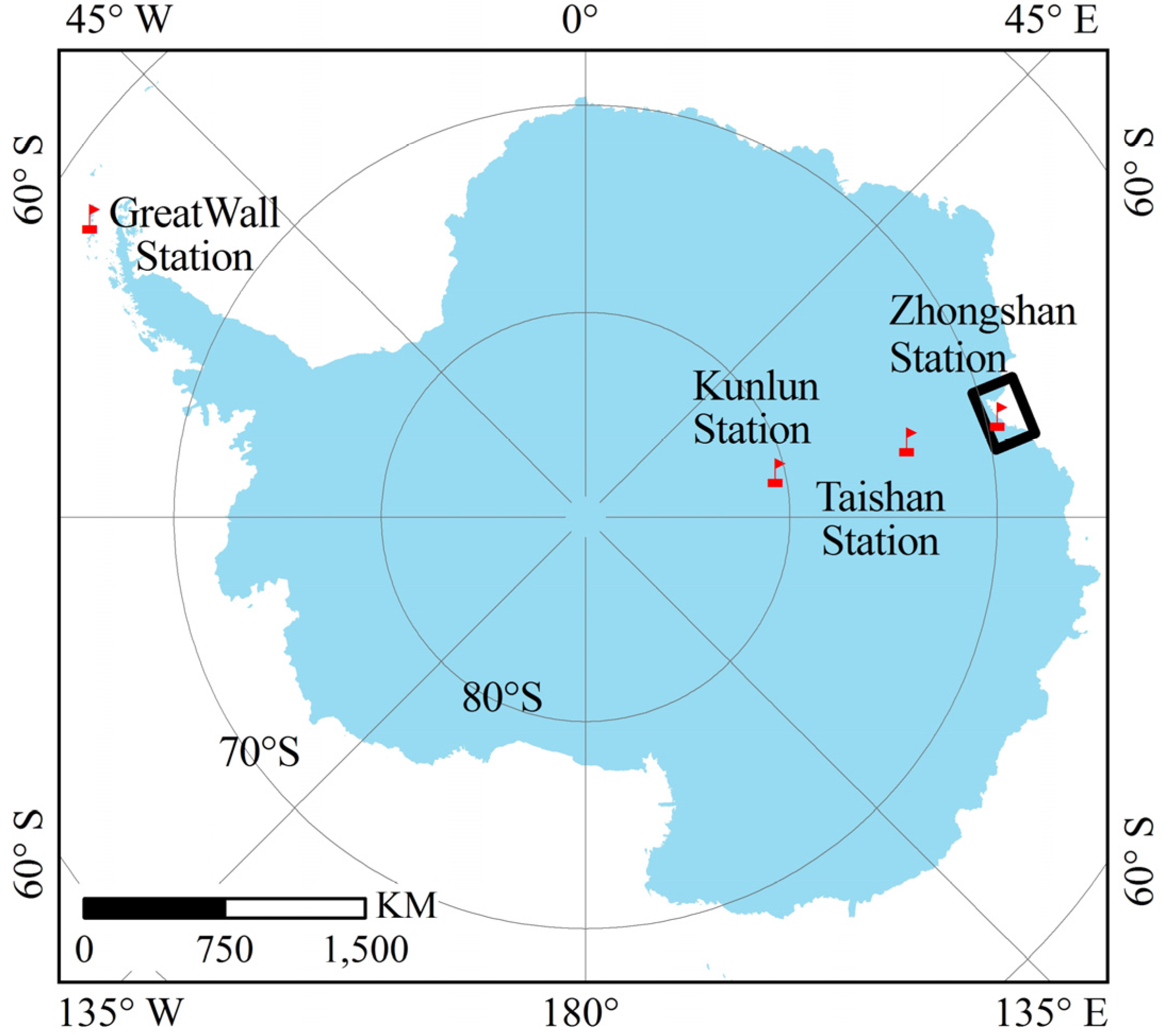
CHINARE began in 1984 and has been carried out successfully for 31 years. Currently, there are four Chinese Research Stations in Antarctica: Great Wall Station (62°12′59″ S, 58°57′52″ W, built in February 1985), Zhongshan Station (69°22′24″ S, 76°22′40″ E, built in February 1989), Kunlun Station (80°25′01″ S, 77°06′58″ E, built in January 2009), and Taishan Station (73°51′50″ S, 76°58′29″ E, built in February 2013) (
Figure 1). The first two stations operate all year, and the latter two stations currently only operate during the austral summer because of severe weather conditions. RV
Xuelong, an icebreaker ice-strengthened to Class B1, is the only Chinese polar scientific research vessel. It was designed to break ice as thick as 1.1 m (including 0.2-m-thick snow) at 1.5 knots. Every year, RV
Xuelong must traverse the pack ice in Prydz Bay (mostly fast ice) in East Antarctica and break through it to reach Zhongshan Station for resupply and staff transfer in late November or early December. In general, the shortest route through fast ice that RV
Xuelong must cross to reach Zhongshan Station in early summer is approximately 10 km. Tidal cracks often appear in fast ice, posing dangers to snow vehicles/snowmobiles along the travel route for resupply from RV
Xuelong to Zhongshan Station.
The study area is the fast ice region near Zhongshan Station in Antarctica (
Figure 1). Fast ice is adjacent to coasts, islands, or grounded icebergs and characterized as motionless unless, for example, it breaks by strong winds [
16]. Its spatiotemporal patterns differ significantly and can extend from a few hundred meters to a few tens of kilometers (although it can reach up to 200 km) [
17,
18]. The extent of the fast ice near Zhongshan Station can be more than 20 km in November, and the maximum ice thickness can reach 1.74 m [
19]. The bathymetry near Zhongshan Station is highly undulated, which can result in icebergs grounding offshore from Zhongshan Station. Both icebergs with different sizes and shapes and the nearby islands off Zhongshan Station allow fast ice to easily form, and tidal cracks are often observed.
3. Data Set and Pre-Processing
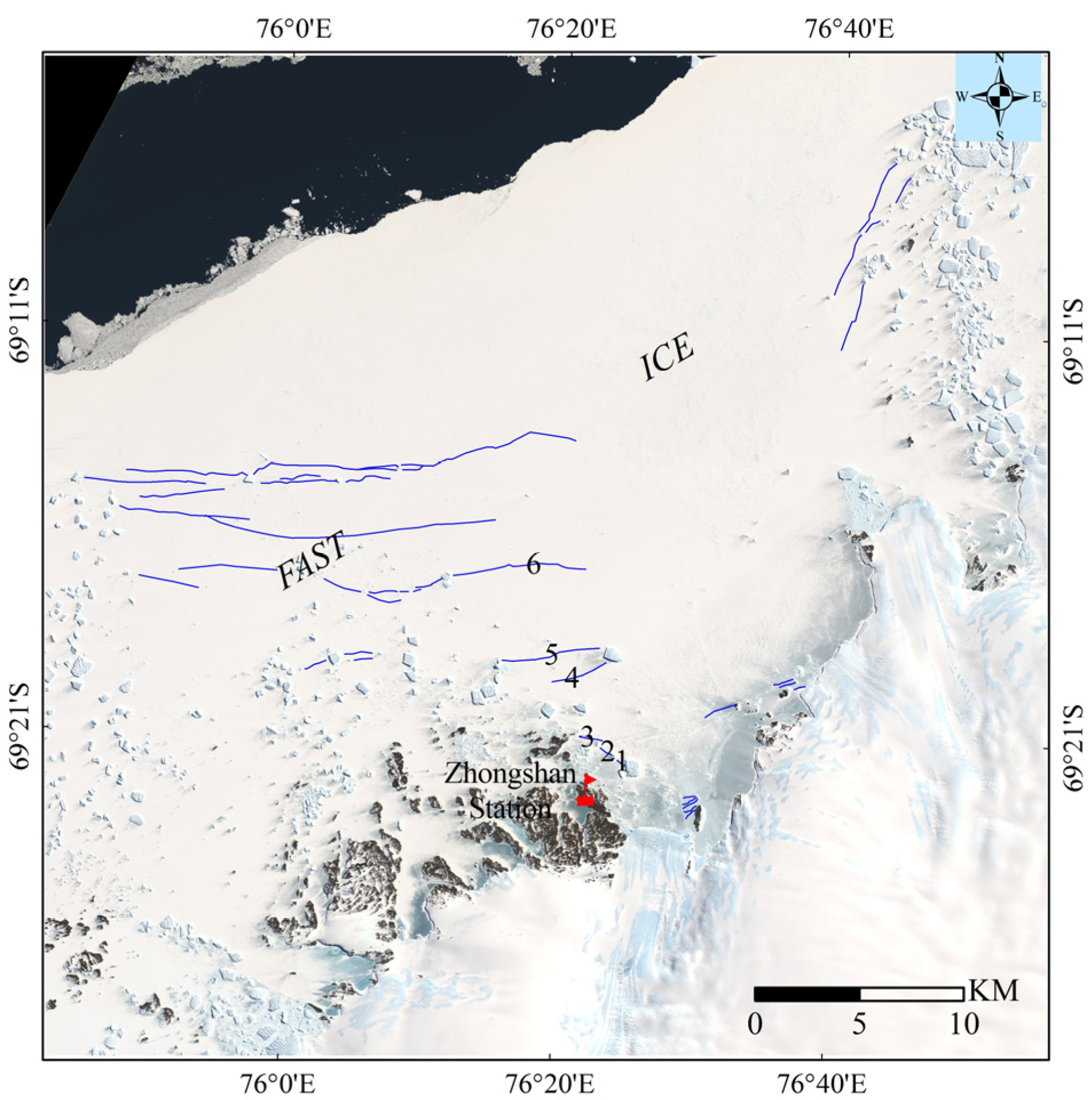
OLI data acquired on 30 November 2014 covering a fast ice region off Zhongshan Station was utilized to detect tidal cracks (
Figure 2). The data were freely downloaded in GeoTIFF format from the U.S. Geological Survey (USGS) website. Images were geometrically and radiometrically corrected and projected in the WGS1984/Antarctic Polar Stereographic Projection. The spectral bands of the OLI sensor are given in
Table 1. In this study, multi-spectral bands in the visible/near-infrared (VNIR) and shortwave infrared (SWIR) spectral bands (Bands 1–7) with a spatial resolution of 30 m, as well as the panchromatic band (Band 8) with a spatial resolution of 15 m, were used for tidal crack detection. The geographic accuracy for OLI data is about 12 m (according to Landsat-8 data products descriptions), which is less than one pixel. The OLI data was processed into top-of-atmosphere (TOA) reflectance according to the Landsat 8 Product specification. To obtain multispectral bands with a resolution of 15 m, the Gram–Schmidt spectral sharpening (GS) method [
20] was employed for data fusion processing. Both the panchromatic sharpening results of Band 1–7 and Band 8 with a resolution of 15 m and the multispectral Band 1–7 with a resolution of 30 m are utilized for tidal crack detections.
The vertical direction gradient data were obtained from the filtered results of OLI data by Sobel vertical direction operator with 3 × 3 windows [
21]. A gradient image represents the change in the pixel values in a given direction. Its most common use is in edge detection. In a gradient image, pixels with the largest gradient values identify edge pixels where the edge can be traced in the direction perpendicular to the gradient direction. In the current study, we found that most tidal cracks are parallel to the coastline in an east-west direction. This is almost parallel to the orientation of the image swath, so the vertical direction gradient data were used as the input image to detect tidal cracks.
Visual extraction of tidal cracks was also implemented using available TOA reflectance and its gradient in the imagery data. Analysis was performed by sea ice experts at Beijing Normal University. In situ measurements were also conducted by wintering personnel of the 30th CHINARE on 30 and 31 October 2014 to identify and validate cracks. The measurements included snow depth, sea ice thickness, crack points location (longitude and latitude), and the approximate length of each crack. Snow depth was measured by a stainless ruler with an accuracy of 0.1 cm, and sea ice thickness was measured by a special gage with an accuracy of 0.1 cm in holes drilled by a Kovacs ice auger (5 cm in diameter). Six tidal cracks with a width of 0.3–1.45 m were obtained from field observations, and 39 tidal cracks were identified from OLI data. The GPS measurements of the six tidal cracks could well coincide with those in the OLI image. Both sets (visually-interpreted cracks from the images and field-observed cracks) were used to evaluate the results from the semi-automatic mapping technique. Tidal prediction data for Zhongshan Station were obtained from the Australian Bureau of Meteorology for the analysis of the influence on the widths of tidal cracks.
4. Method
4.1. Manual Detection of Tidal Cracks in the Images
Tidal cracks were detected manually in each one of the two OLI imagery data sets—the 15- and 30-m-resolution sets. The process involved manual interpretation of the images yet supported by field observations. It should be noted that narrow cracks may not be readily visible in the images since the resolution of the imagery data is coarser than the crack width. For this reason, field observations are used to confirm identification of those cracks which can hardly be seen in the image. Eventually, all cracks were identified manually in the images.
Figure 2 is a false color OLI image (RGB assigned to bands 4, 3 and 2) at 30-m resolution, representing fast ice in the Prydz Bay. Manually detected tidal cracks are overlaid (blue lines). Two buffers were established using ArcGIS 10.0 software (ESRI In, Redlands, CA, USA); one included the detected crack pixels in the 15-m-resolution images and the other included the pixels in the 30-m-resolution images. In order to tolerate errors in the geo-location of the pixels, each buffer was enlarged to accommodate 3 pixels surrounding each detected pixel. Hence, the first and the second buffers tolerated errors within a width of 45 and 90 m, respectively.
4.2. The Automatic Lineament Extraction Algorithm
An edge in an image represents a sharp local change in the image intensity, usually associated with a discontinuity (or equivalently high first derivative of the image intensity). Its shape usually depends on the geometrical and optical properties of the object, the illumination conditions, and the noise level in the images [
22]. Tidal cracks can be considered edges because the seawater or the refrozen (new) ice within the crack can induce a difference in the spectral reflectance or backscatter density compared to the surrounding fast ice. This is how a tidal crack can be visually or automatically identified in remote sensing images even as at a subpixel level, albeit with inherent uncertainties.
Previous studies have demonstrated good results in mapping linear discontinuities from satellite images [
23,
24,
25,
26]. The automatic lineament extraction algorithm in Geomatica 2015 software, integrated in the LINE module, was used in this study. The algorithm employs the Canny method [
27], which is one of the most sucessful methods for edge detection. Its success can be attributed to its performance according to three criteria of excellent detection: low error rate, good localization, and single response to an edge. The Canny algorithm has proven to detect edges under almost all scenarios compared to the Prewitt, Sobel, and LOG (Laplacian of Gaussian) algorithms [
28].
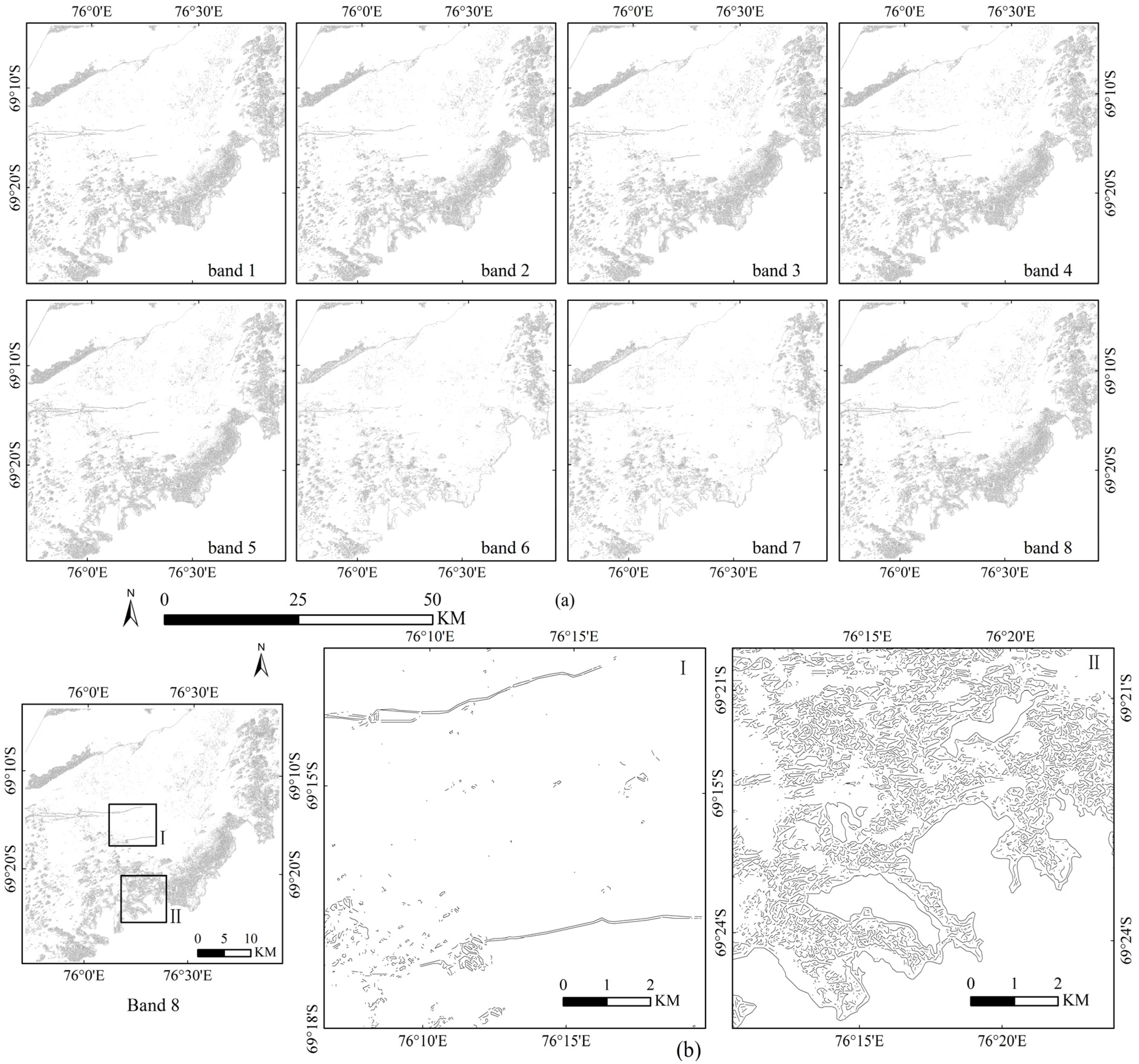
There are three processing stages in the LINE module: edge detection, thresholding, and curve extraction. In the first stage, the Canny edge detection algorithm is applied to produce an edge strength image, including smoothing the input image with a Gaussian filter function, computing the gradient filtered image, and suppressing the pixels whose gradients are not the local maximum (by setting the edge strength to 0). In the second stage, a threshold on edge strength is set to obtain a binary image. Each non-zero pixel in the binary image represents an edge element. In the third stage, curves are extracted from the binary edge image. This step consists of several sub-steps. Initially, a thinning algorithm is applied to the binary edge image to produce pixel-wide skeleton curves. Next, a sequence of pixels for each curve is extracted from the image. Any curve with a number of pixels less than a given threshold for curve length is discarded from further processing. The extracted curve is then converted to vector form by fitting piecewise line segments to it. The resulting polyline is an approximation of the original curve, where the maximum fitting error is specified by the line fitting error. Finally, the algorithm links pairs of polylines that satisfy the following criteria: (1) that end segments of the two polylines face each other and have similar orientations (the angle between the two segments is less than the threshold for angular difference); and (2) that end segments are close to each other (the distance between the end points is less than the threshold for linking distance).
The OLI data are first scaled down to 8-bit data from 16-bit using a minimum-maximum linear contrast stretch and then masked using a coastline and rock dataset from the Scientific Committee on Antarctic Research (SCAR) Antarctic Digital Database (ADD) (
http://www.add.scar.org/), leaving the fast ice region, open ocean and pack ice as the input image for tidal crack detection. Both TOA reflectance data and vertical direction (90 degrees) gradient data from Bands 1–8 with resolutions of 15 m, and the TOA reflectance data and vertical direction gradient data from Bands 1–7 with resolutions of 30 m are processed using the LINE module.
The parameters in the LINE module are same for all input data. The filter radius value is 3 pixels (a large value can result in less noise but much less detail detected), while the edge gradient value is also 3 pixels (a large value can create sparse pixels in the edge image influencing the subsequent lineament extraction process). The curve length threshold is 3 pixels and the angular difference threshold is 75 degrees (the value defines the maximum angle between two vectors that can be linked to form an edge segment). The threshold of the linking distance between edge segments is 3 pixels (the value specifies the maximum distance between two vectors for them to be linked). All parameters except for the angular difference threshold are suitable to obtain enough details about the edge, and the angular difference threshold set to be as 75 degree is to obtain longer detected line segments.
4.3. Automated Tidal Crack Identification and Detection
In the manually interpreted image in
Figure 2, only three tidal cracks are found to be shorter than 500 m, and more than two-thirds of the detected cracks are longer than 1000 m. Therefore, in this study, detected lines with lengths greater than 500 m are used for tidal crack identification. The steps of the automated tidal crack detection proceed as follows. An overlay analysis is conducted between the detected lines output from the LINE module and the buffer data (including the manually extracted cracks). A topology check is then carried out between the two sets. A detected line should be accepted as a tidal crack if its length is >500 m and extends parallel to or overlaying the manually interpreted tidal cracks. The latter condition means that the points lie within the buffer pointed out in
Section 4.1 (
i.e., being within 3 pixels from the manually extracted crack). When more than one line is found in the same location, the longest line is retained. The performance of the automated detection technique is evaluated by comparing the number, maximum length, and total length of detected lines against the results from the manually interpreted lines. This was done for both data sets (15 m and 30-m resolution) and for data from each spectral band.
5. Results
5.1. Input Data with a Spatial Resolution of 15 m
5.2. Input Data with a Spatial Resolution of 30 m
The results from the data with a resolution of 15 and 30 m are similar. The statistics of the detected lines for the 30-m resolution are presented in
Table 5 and
Table 6 using the two sets of input data as shown. In the TOA reflectance data results, Bands 3–5 have almost the same line detection capabilities as Bands 1–2. In the vertical direction gradient data results, Band 5 detected the most lines, followed by Band 4 and Bands 1–3. When using the vertical direction gradient data with a resolution of 30 m, Bands 6–7 detect approximately the same number of lines as Bands 1–5; the line detection performances of Bands 6–7 improved compared with the results calculated using the data with a resolution of 15 m (
Table 4 and
Table 6).
Table 7 shows that the fewest tidal cracks longer 1000 m were detected in Bands 6–7 in both the TOA and vertical direction gradient data. Bands 4 and 5 performed the best, followed by Bands 2–3 and Band 1. In
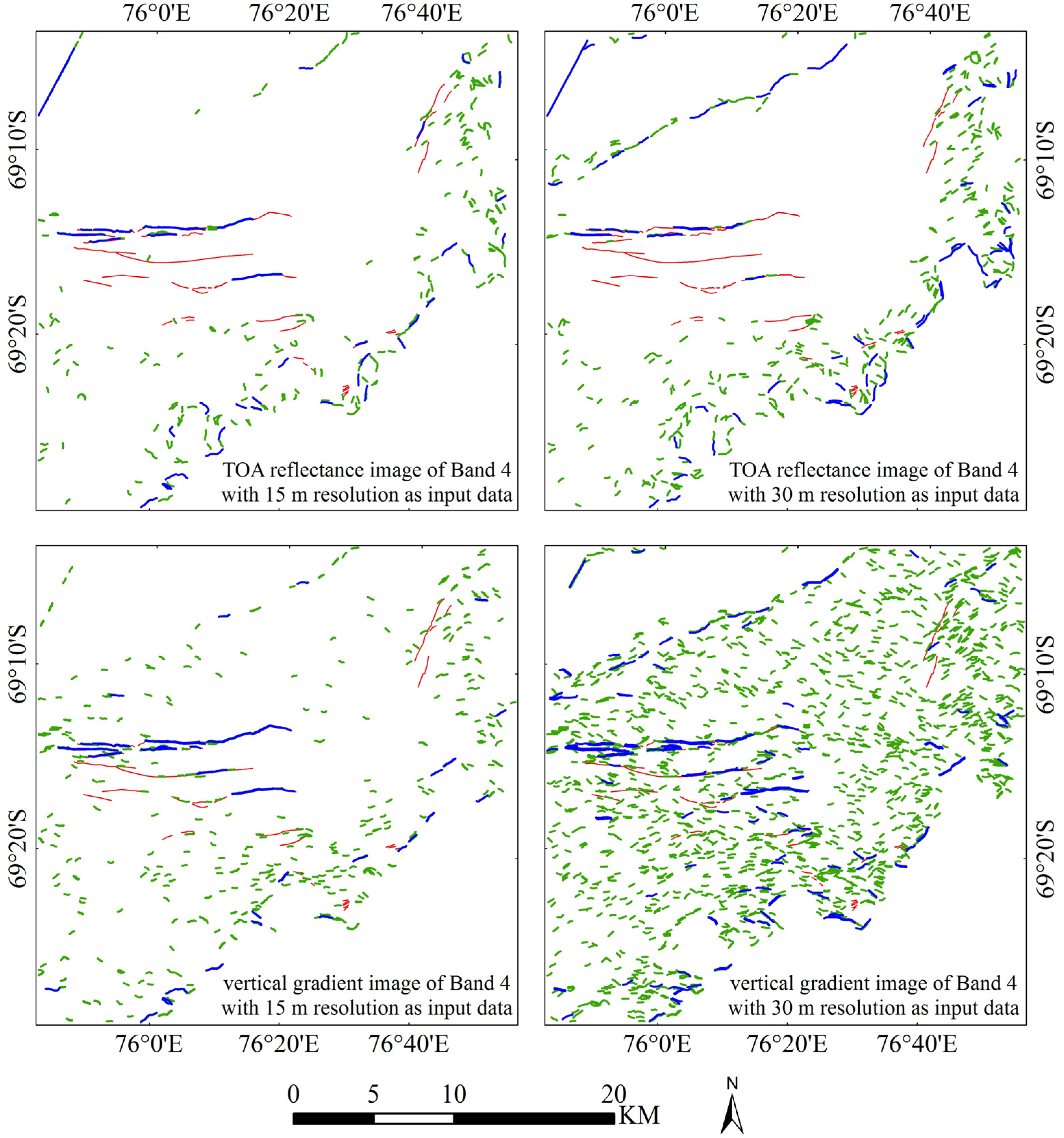
Table 7, the ratio of the length of detected tidal cracks to the total length of interpreted tidal cracks in the vertical direction gradient data is at least 2.5 times higher than that in TOA reflectance images, and the ratios in Band 5 performed best with about 47.43 and 17.8 percent in the vertical direction gradient data and TOA reflectance images, respectively. In Bands 6–7, many of the detected lines with lengths greater than 500 m are part of the fast ice region boundary, which cannot be used for tidal crack detection. This was also observed in the other bands. For instance, results using Band 4 data with a resolution of 30 m detects many boundary edges (
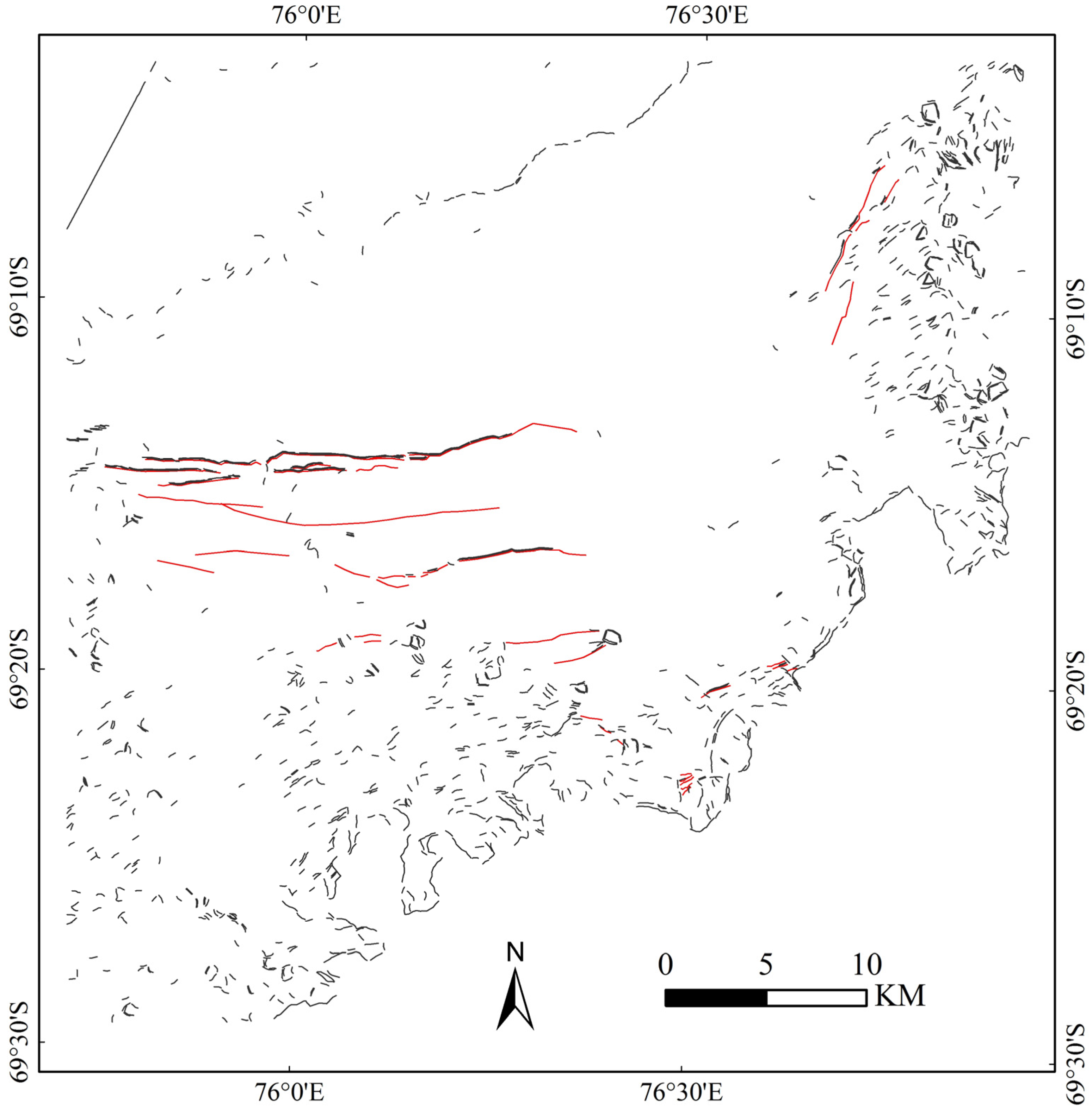
Figure 4). This behavior can be considered an impact of image resampling from a resolution of 15 m to a resolution of 30 m, and the boundary of the fast ice region could be easily detected.
6. Validation Analysis
The process of assigning detected lines to be tidal cracks has been stated in the Method section. The visually interpreted tidal cracks are an integral long line (manually drawn). In the LINE module, the input parameters are smaller (3 pixels), which provides more details and identifies more tidal cracks than what is found in the visual identification. Tidal cracks detected by the LINE module may be short and discontinued segments. Statistics of detected tidal cracks with lengths greater than 500 m are given in
Table 8. A comparison of detected tidal cracks against those from field measurements is given in
Table 9. The number of detected tidal cracks using vertical direction gradient data is more than that using the TOA reflectance images (
Table 8), and the number in the 15-m-resolution data is more than that in the 30-m-resolution data. The maximum number of detected tidal cracks from the 15 and 30-m-resolution data is found in bands 8 and 5, respectively.
The number of detected tidal cracks is different in
Table 8 and
Table 9. Although Band 8 in the results from the 15-m-resolution data and Band 5 in the results from the 30-m-resolution data offer the best results, other bands such as Band 1 and 3 in the 15-m-resolution data also demonstrate the same number as in Band 8. Tidal cracks labeled 4–6 are detected by most bands, and tidal cracks labeled 1–2 are seldom detected by most bands. This may be related to differences of spectral information between bands.
7. Discussion
In the results obtained from 15-m-resolution Bands 1–8, the number of detected line segments from using the vertical direction is higher than the number from using the TOA data by a factor ranging between 4.11 and 5.78. The number of lines longer than 300 m in the results from using the vertical gradient are at least twice the number from using the TOA data (at most 3.25 times), and the number of lines with lengths greater than 1000 m is at least equal that from the TOA data (at most 1.65 times). A greater number of line segments can increase the likelihood of tidal crack detection (
Table 2 and
Table 4). When tidal cracks are greater than 1000 m, the capabilities of the vertical direction gradient data are much better than those of the TOA data, not only in terms of the detected number but also in the total length (
Table 3). It can be found in
Table 3 that Band 5 has the most improved performance due to the gradient operator, with an 85% increase in number and 82.6% increase in total length. The maximum length of a single tidal crack detected using the vertical direction gradient data in Bands 1–3 increased by 16.5%–37.1% compared to the TOA data but decreased in Bands 4–5 and 8, especially in Band 4, which decreased in length by 21%. This means that the vertical direction gradient data detect more of the actual tidal cracks that are confirmed from the visual analysis of the images.
The shapes and lengths of the tidal cracks detected using the vertical direction gradient data are better than those detected using the TOA data.
Figure 4 shows that the tidal cracks detected using the TOA data are portions of the manually-interpreted tidal cracks. On the other hand, some are complete in the vertical direction gradient results. This proves once again that the tidal crack detection capabilities of the vertical direction gradient data are much better than those of the TOA data, in spite of the greater noise level (line segments less than 300 m) and computational time cost (it took 3 min and 10 s to process the vertical direction gradient and TOA data, respectively).
Table 5,
Table 6 and
Table 7 show that, when using the data with a resolution of 30 m, the line detection capability and tidal crack detection capability of the vertical direction gradient data are much better than those of the TOA data.
Tidal cracks could be detected using OLI data with resolutions of 15 m and 30 m, but the results are different. As shown in
Table 2 and
Table 4,
Table 5 and
Table 6, the lines detected using the data with a resolution of 15 m are 3.9–4.5 times longer than those detected using the data with a resolution of 30 m. However, only 68.4%–74.4% as many lines with lengths greater than 300 m were detected using the TOA data with a resolution of 15 m compared with the TOA data with a resolution of 30 m, and only 45.9%–60.8% as many lines were detected using the vertical direction gradient data with a resolution of 15 m compared with a resolution of 30 m. However, the data with a resolution of 15 m had better performance for the detection of tidal cracks than the data with a resolution of 30 m (
Table 3 and
Table 7). For the tidal cracks detected using the TOA data with a resolution of 15 m, the number and total length are both more than 50% of the values detected using the data with a resolution of 30 m. In the tidal cracks detected using the vertical direction gradient data with a resolution of 15 m, the number and total length are also better than those detected using the data with a resolution of 30 m. More importantly, the detected tidal cracks are more complete when using the data with a resolution of 15 m than 30 m (
Figure 4).
There is a significant level of noise in the results, which is related to the large number of icebergs with textures and shadows in the study area. Icebergs in this region are mostly calved from the Dalk Glacier and Flatnes Ice Tongue east of Zhongshan Station, which are often grounded there because of the bathymetric features. The “noise” in the line detection results is due to the different shapes, textures, and shadows of the icebergs. There may be much less “noise” in the line detection results if new approaches are developed to reduce the strong noise. Tidal cracks between icebergs or islands could not be well detected because there is too much noise, and there are small cracks that are short and narrow. At the same time, the smoothness of the fast ice also has a large influence on tidal crack identification. The surface of fast ice is usually smooth, but here there are many icebergs in the study area. This results in smooth to rough textures in the satellite images. Rough texture can be a manifestation of noise, which will influence tidal crack identification during line detection.
The tidal crack width can be strongly influenced by daily and monthly tidal stages (tidal zone dynamics). Predictions of tidal elevations for Zhongshan Station from the Australian Bureau of Meteorology indicated that there was a neap tide on 30 November 2014, and spring tides occurred on 25–26 November and 8–9 December 2014. In the study area, neap tides have a weak influence on the widths of tidal cracks. Typical tidal crack width in winter is remarkably narrower than the OLI resolution, which means that the tidal crack edge information is not sufficient for identification. Tidal cracks are wider in the spring, which makes it more conductive to identification in satellite images.
Tidal cracks can be identified using satellite images with high spatial resolutions (less than 1 m), such as QuickBird, Ikonos, and Worldview-1 [
9]. What about satellite images with medium-coarse spatial resolution data? There are two conditions that must be considered for satellite images to identify tidal cracks: The first is a spatial resolution that allows for the detection of the narrowest tidal cracks, and the second is a swath that covers a wide enough area. This will facilitate the generation of statistics over large areas. This study has demonstrated that images with resolutions of 30 m can be used to identify tidal cracks. If the satellite images have coarse spatial resolutions (greater than 30 m) the success of the results will be rather limited.
8. Conclusions
In this study, tidal cracks in the fast ice region near Zhongshan Station in East Antarctica were semi-automatically extracted using the LINE module of Geomatics 2015 software with input from Landsat-8 OLI data with resolutions of 15 and 30 m. The module identifies linear edges. The length of the line is used as a condition to identify tidal cracks while the match with crack lines identified in the images and verified in field observations constitutes another important condition. A comparison of results from using the TOA reflectance data and vertical direction gradient of the images was conducted. Results indicated that the ratio of the length of detected tidal cracks to the total length of interpreted tidal cracks in the vertical direction gradient data is much higher than that in TOA reflectance images with the same resolution, and the ratio in data with a resolution of 15 m is much higher than that in data with a resolution of 30 m. The statistics also showed that, in the results from 15-m data, the ratios in Band 8 performed best with about 50.92 and 31.38 percent when using the vertical direction gradient data and TOA reflectance images, respectively, and in the results from the 30-m-resolution data, the ratios in Band 5 performed best with about 47.43 and 17.8 percent in the vertical direction gradient data and TOA reflectance images, respectively. There was noise in the results related to the presence of icebergs in this region. There are a large number of icebergs with textures and shadows in the region influencing the data processing by the algorithm. Therefore, in combination with manual steps, the semi-automatic mapping of tidal cracks has been achieved using the LINE module based on the Canny algorithm. This study supports efforts of field investigations of marine mammals and hunting destinations, and provides methods for the identification of hazardous regions along travel routes in fast ice regions.
Acknowledgments
This work was supported by the Chinese Arctic and Antarctic Administration, National Natural Science Foundation of China (Grant No. 41106157), the National Basic Research Program of China (Grant No. 2012CB957704), the Specialized Research Fund for the Doctoral Program of Higher Education (Grant No. 20120003110030), the Chinese Polar Environment Comprehensive Investigation, Assessment Program, and Public Welfare Project of the State Oceanic Administration (201205007) and the Project of International Cooperation and Exchanges CHINARE (IC201302). PH was supported by Australian Antarctic Science grant 4072 and 4301, as well as by the Antarctic Climate and Ecosystems CRC program. We are grateful to USGS for providing Landsat-8 OLI data and to the Australian Bureau of Meteorology for providing tide prediction data. We would like to thank the anonymous reviewers for their valuable comments.
Author Contributions
F.H. conceived and designed the experiments, and wrote the manuscript; X.L., T.Z. and Y.L. processed and analyzed the data; J.Z collected field data and discussed the results; M.S. and P.H. investigated the results and revised the manuscript; S.L. and X.C. investigated the results, revised the manuscript and supervised this study.
Conflicts of Interest
The authors declare no conflict of interest.
References
- Volkov, V.A.; Johannessen, O.M.; Borodachev, V.E.; Voinov, G.N.; Pettersson, L.H.; Bobylev, L.P.; Kouraev, A.V. Polar Seas Oceanography: An Integrated Case Study of the Kara Sea; Springer: London, UK, 2002; pp. 238–247. [Google Scholar]
- Tschudi, M.A.; Curry, J.A.; Maslanik, J.A. Characterization of springtime leads in the beaufort/chukchi seas from airborne and satellite observations during fire/sheba. J. Geophys. Res. Oceans 2002, 107, 8034. [Google Scholar] [CrossRef]
- Moore, C.W.; Obrist, D.; Steffen, A.; Staebler, R.M.; Douglas, T.A.; Richter, A.; Nghiem, S.V. Convective forcing of mercury and ozone in the arctic boundary layer induced by leads in sea ice. Nature 2014, 506, 81–84. [Google Scholar] [CrossRef] [PubMed]
- Siniff, D.B.; DeMaster, D.P.; Hofman, R.J.; Eberhardt, L.L. An analysis of the dynamics of a weddell seal population. Ecol. Monogr. 1977, 47, 319–335. [Google Scholar] [CrossRef]
- Kooyman, G. Marine mammals and emperor penguins: A few applications of the krogh principle. Am. J. Physiol. Regul. Integr. Comp. Physiol. 2015, 308, R96–R104. [Google Scholar] [CrossRef] [PubMed]
- Watanuki, Y.; Kato, A.; Naito, Y.; Robertson, G.; Robinson, S. Diving and foraging behaviour of Adélie penguins in areas with and without fast sea-ice. Polar Biol. 1997, 17, 296–304. [Google Scholar] [CrossRef]
- Takahashi, A.; Sato, K.; Nishikawa, J.; Watanuki, Y.; Naito, Y. Synchronous diving behavior of Adélie penguins. J. Ethol. 2004, 22, 5–11. [Google Scholar] [CrossRef]
- MANICE. Manual of Standard Procedures for Observing and Reporting Ice Conditions 2005. Available online: https://ec.gc.ca/glaces-ice/4FF82CBD-6D9E-45CB-8A55-C951F0563C35/MANICE.pdf (accessed on 16 July 2015).
- Shokr, M.; Sinha, N. Sea Ice: Physics and Remote Sensing; Wiley: Hoboken, NJ, USA, 2015; pp. 75–77, 391. [Google Scholar]
- Wang, X.; Cheng, X.; Hui, F.M.; Cheng, C.; Liu, Y.; Sum, H.K. Xuelong navigation in fast-ice near the Zhongshan Station, Antarctica. Mar. Technol. Soc. J. 2014, 48, 84–91. [Google Scholar] [CrossRef]
- Leppäranta, M. The Drift of Sea Ice; Springer: New York, NY, USA, 2011; Volume 90. [Google Scholar]
- Hirose, T.; Vachon, P.W. Demonstration of ERS tandem mission SAR interferometry for mapping land fast ice evolution. Can. J. Remote Sens. 1998, 24, 89–92. [Google Scholar] [CrossRef]
- Quackenbush, L.J. A review of techniques for extracting linear features from imagery. Photogramm. Eng. Remote Sens. 2004, 70, 1383–1392. [Google Scholar] [CrossRef]
- Hashim, M.; Ahmad, S.; Johari, M.A.M.; Pour, A.B. Automatic lineament extraction in a heavily vegetated region using landsat enhanced thematic mapper (ETM+) imagery. Adv. Space Res. 2013, 51, 874–890. [Google Scholar] [CrossRef]
- Turker, M.; Kok, E.H. Field-based sub-boundary extraction from remote sensing imagery using perceptual grouping. ISPRS J. Photogramm. Remote Sens. 2013, 79, 106–121. [Google Scholar] [CrossRef]
- WMO. Wmo Sea-Ice Nomenclature: Terminology, Codes, Illustrated Glossary and Symbols; Secretariat of the World Meteorological Organization: Geneva, Switzerland, 1970. [Google Scholar]
- Giles, A.B.; Massom, R.A.; Lytle, V.I. Fast-ice distribution in east antarctica during 1997 and 1999 determined using radarsat data. J. Geophys. Res. Oceans 2008, 113, 15. [Google Scholar] [CrossRef]
- Mahoney, A.R.; Eicken, H.; Gaylord, A.G.; Gens, R. Landfast sea ice extent in the chukchi and beaufort seas: The annual cycle and decadal variability. Cold Reg. Sci. Technol. 2014, 103, 41–56. [Google Scholar] [CrossRef]
- Lei, R.; Li, Z.; Zhang, Z.; Cheng, Y.; Dou, Y. Summer fast-ice evolut ion off Zhongshan Station, Antarct Ica. Chin. J. Polar Res. 2007, 19, 275–283. (In Chinese) [Google Scholar]
- Laben, C.A.; Brower, B.V. Process for Enhancing the Spatial Resolution of Multispectral Imagery Using Pan-Sharpening. U.S. Patent 6011875, 2000. Available online: http://www.google.com/patents/US6011875 (accessed on 16 July 2015). [Google Scholar]
- Vincent, O.; Folorunso, O. A Descriptive Algorithm for Sobel Image Edge Detection. In Proceedings of the Informing Science & IT Education Conference (InSITE), Macon, GA, USA, 12–15 June 2009; pp. 97–107.
- Marr, D.; Hildreth, E. Theory of edge detection. Proc. R. Soc. Lond. Ser. B Biol. Sci. 1980, 207, 187–217. [Google Scholar] [CrossRef]
- Kocal, A.; Duzgun, H.; Karpuz, C. Discontinuity Mapping with Automatic Lineament Extraction from High Resolution Satellite Imagery. Available online: http://www.isprs.org/proceedings/XXXV/congress/comm7/papers/205.pdf (accessed on 16 July 2015).
- Hung, L.Q.; Batelaan, O.; De Smedt, F. Lineament Extraction and Analysis, Comparison of Landsat Etm and Aster Imagery. Case Study: Suoimuoi Tropical Karst Catchment, Vietnam. Available online: http://spie.org/Publications/Proceedings/Paper/10.1117/12.627699 (accessed on 16 July 2015).
- Ramli, M.F.; Yusof, N.; Yusoff, M.K.; Juahir, H.; Shafri, H. Lineament mapping and its application in landslide hazard assessment: A review. Bull. Eng. Geol. Environ. 2010, 69, 215–233. [Google Scholar] [CrossRef]
- Rahnama, M.; Gloaguen, R. Teclines: A MATLAB-based toolbox for tectonic lineament analysis from satellite images and DEMs, part 2: Line segments linking and merging. Remote Sens. 2014, 6, 11468–11493. [Google Scholar] [CrossRef]
- Canny, J. A computational approach to edge detection. IEEE Trans. Pattern Anal. Mach. Intell. 1986, PAMI-8, 679–698. [Google Scholar] [CrossRef]
- Maini, R.; Aggarwal, H. Study and comparison of various image edge detection techniques. Int. J. Image Process. 2009, 3, 1–11. [Google Scholar]
© 2016 by the authors; licensee MDPI, Basel, Switzerland. This article is an open access article distributed under the terms and conditions of the Creative Commons by Attribution (CC-BY) license (http://creativecommons.org/licenses/by/4.0/).


 ,
, 

