A Symmetric Sparse Representation Based Band Selection Method for Hyperspectral Imagery Classification

Abstract

A novel Symmetric Sparse Representation (SSR) method has been presented to solve the band selection problem in hyperspectral imagery (HSI) classification. The method assumes that the selected bands and the original HSI bands are sparsely represented by each other, i.e., symmetrically represented. The method formulates band selection into a famous problem of archetypal analysis and selects the representative bands by finding the archetypes in the minimal convex hull containing the HSI band points (i.e., one band corresponds to a band point in the high-dimensional feature space). Without any other parameter tuning work except the size of band subset, the SSR optimizes the band selection program using the block-coordinate descent scheme. Four state-of-the-art methods are utilized to make comparisons with the SSR on the Indian Pines and PaviaU HSI datasets. Experimental results illustrate that SSR outperforms all four methods in classification accuracies (i.e., Average Classification Accuracy (ACA) and Overall Classification Accuracy (OCA)) and three quantitative evaluation results (i.e., Average Information Entropy (AIE), Average Correlation Coefficient (ACC) and Average Relative Entropy (ARE)), whereas it takes the second shortest computational time. Therefore, the proposed SSR is a good alternative method for band selection of HSI classification in realistic applications.

1. Introduction

Thanks to the powerful advantage in collecting both spectrum and images of ground objects on the earth surface, hyperspectral imaging is a popular technique in many application fields, including environment monitoring [1,2], precision agriculture [3,4], mine exploration [5,6] and so on. However, many challenging problems exist in the hyperspectral imagery (HSI) processing, especially the “curse of dimensionality” [7,8,9]. The problem results from numerous bands and strong intra-band correlations and it indicates that achieving higher classification accuracy requires more training samples. However, collecting too many training samples is expensive and time-consuming [10,11]. Therefore, dimensionality reduction is an alternative way to conquer the above problem and to promote the applications of HSI data.

Usually, dimensionality reduction can be classified into two main groups: band selection and feature extraction [12,13]. Feature extraction reduces the dimensionality of HSI data through transforming it into a low-dimensional feature space, whereas band selection selects a proper band subset from the original band set [14,15]. In this study, we focus on band selection because we believe band selection inherits the original spectral meanings of HSI data when compared to feature extraction.

The research history of band selection starts from the birth of hyperspectral imaging technique. Many classical methods from information theory were introduced into the hyperspectral community. The entropy-based methods select a band subset aiming for maximal information entropy or relative entropy [16,17]. The effects from intra-band correlations are usually neglected in the entropy-based methods, and the representative bands are prone to be highly correlated and do not necessarily perform well in realistic applications [18]. Meanwhile, intra-class divergences can be maximized to formulate the distance measure based methods using Euclidean, Spectral Information Divergence (SID), Mahalanobis distances and so on [18,19]. The methods outperform the entropy-based methods in many instances but the selected band subsets vary greatly across different distance measurements. In addition, some measurements such as Spectral Angle Mapping (SAM) do not consider the intra-band correlations and these methods might bring about unstable results in band selection. The intra-band correlation based methods select a proper band subset that has minimal band correlations, and typical examples are the mutual information method [20], the joint band-prioritization and band-decorrelation method [21], the semi-supervised band clustering method [22] and the column subset selection method [23]. These methods perform better than all classical methods, but they rely heavily on prior knowledge of intra-band and still have some respective disadvantages. For example, the band clustering algorithms typically involve complex combinatorial optimization leading to a plethora of heuristics, and the choices of clustering centers highly affect the result of representative bands [22].

With the maturity of artificial intelligence, many relevant algorithms have been adopted to solve the band selection problem. The particle swarm optimization based methods implement a defined iterative searching criterion function to obtain a proper band subset that maximizes the intra-class separabilities. Typical algorithms are the simple particle swarm optimization algorithm using the searching criterion function of minimum estimated abundance covariance [24], the parallel particle swarm optimization algorithm [25], and the improved particle swarm optimization algorithm [26]. The particle swarm optimization based methods have lower computational complexity and smaller parameter tuning works, but the methods are easily encountered in local minima and could not guarantee successful global optimization. The ant colony optimization based methods implement a positive feedback scheme and continually update the pheromones to optimize the band subset combination. The representative algorithms are the parallel ant colony optimization algorithm [27] and the specific ant colony algorithm for urban data classification [28]. Because they lack sufficient initial information, the ant colony based methods usually take long computational times to obtain a stable optimal solution. The complex networks based methods input the HSI dataset into complex networks and find an appropriate band subset that has best qualification for differentiating all ground objects [29,30]. The band subset from complex networks performs better in identifying different ground objects than classical methods, whereas the high computational complexity in constructing and analyzing the complex network hinders its applications in realistic works. Other artificial intelligence based methods in recent literature include the progressive band selection method [31], the constrained energy minimization based method [32] and the supervised trivariate mutual information based method [33]. From the above, most artificial intelligence based methods could not perfectly balance the computational speeds and the optimization solutions. In addition, the estimated band subset is difficult to physically interpret because of the complicated searching strategy adopted.

More recently, the popularity of compressive sensing brings about new perspectives for band selection and many sparsity-based algorithms have been presented in the literature [34,35,36]. The sparsity theory states that each band vector (i.e., the hyperspectral image in each band is reshaped as a band vector in the column format) can be sparsely represented using only a few non-zero coefficients in a proper basis or dictionary [37,38]. Sparse representation could uncover underlying features within the HSI band collection and help selecting a proper band subset. The Sparse Nonnegative Matrix Factorization (SNMF) based methods originate from the idea of “blind source separation”, and simultaneously factorize the HSI data matrix into a dictionary and a sparse coefficient matrix [36]. The band subset is then estimated from the sparse coefficient matrix. The examples of SNMF based methods are the improved SNMF with thresholded earth’s mover distance algorithm [39] and the constrained nonnegative matrix factorization algorithm [40]. The SNMF based methods stand on low rank approximations and have a great degree of flexibility in capturing the variances among different band vectors. Unfortunately, the band subset from SNMF based methods can be hard to interpret and its physical or geometric meaning is unclear. Different from the SNMF based methods, the dictionaries in sparse coding based methods are learned or manually defined in advance. The sparse coding based methods integrate the regular band selection models with sparse representation model of band vectors to estimate the proper representative bands. Typical methods are the sparse representation based (SpaBS) method [35], the sparse support vector machine method [41], the sparse constrained energy minimization method [42], the discriminative sparse multimodal learning based method [43], the multitask sparsity pursuit method [44] and the least absolute shrinkage and selection operator based method [45]. Similar with SNMF, the band subset from sparse coding has unclear physical or geometric explanations. When the dictionary in sparse coding is set to be equal to the HSI data matrix, all band vectors can be assumed to be sampled from several independent subspaces and the Sparse Subspace Clustering (SSC) model is then formulated. Typical methods include the collaborative sparse model based method [34] and the Improved Sparse Subspace Clustering (ISSC) method [46]. The SSC based methods combine the sparse coding model with the subspace clustering approach, and the benefit of clustering renders that the achieved band subset is easy to interpret. Nevertheless, the clustering center in the methods is difficult to uniquely determine because it depends on the number of clusters.

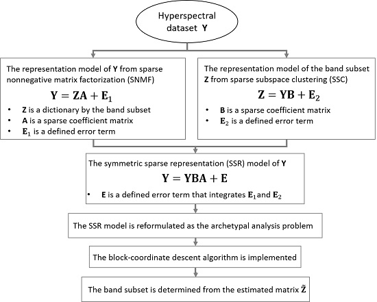
In this study, different from previous works, a Symmetric Sparse Representation (SSR) method is proposed to investigate the band selection problem. The aim of SSR is to combine the advantages of SNMF and SSC, while avoiding their respective disadvantages. Compared with the SNMF and SSC, the SSR method favors the following three main innovations:

(1)

SSR combines the assumptions of SNMF and SSC and integrates benefits from both methods. The SNMF regards that each band vector can be sparsely represented by the aimed band subset with a sparse and nonnegative coefficient vector, and it explains that each band vector in HSI data can be regarded as a convex combination of the aimed band subset, even though the band subset is undetermined. The SSC assumes that each selected band vector can be sparsely represented in the feature space spanned by all the band vectors, and each selected band vector is a convex combination of all the band vectors in HSI data. The SSR combines symmetric assumptions of both SNMF and SSC together, and then it could integrate the advantages of SNMF and the virtues of SSC.

(2)

The SSR method has clearer geometric interpretations than many current methods. SSR formulates the band selection problem into the optimization program of archetypal analysis. Archetypal analysis gives the SSR a clear geometric meaning that selecting the representative bands is to find archetypes (i.e., representative corners) of the minimal convex hull containing the HSI band points (i.e., a band vector corresponds to a high-dimensional band point). In contrast, the current sparsity-based methods including SNMF and sparse coding based method could capture low-rank feature of HSI band set, but the meanings of selected bands are difficult to interpret [47].

(3)

The SSR method does not involve any tuning works of inner parameters and this feature makes it easier to implement SSR in realistic applications. Particularly, the SSR does not have the clustering procedure, and hence the estimated SSR band subset avoids negative effects from the clustering approaches that exist in SNMF and SSC.

The rest of this paper is organized as follows. Section 2 presents the band selection procedure using the proposed SSR method. Section 3 describes experimental results of SSR in band selection for classification on two widely used HSI datasets. Section 4 discusses the performance of SSR compared to four other methods. Section 5 states the conclusions.

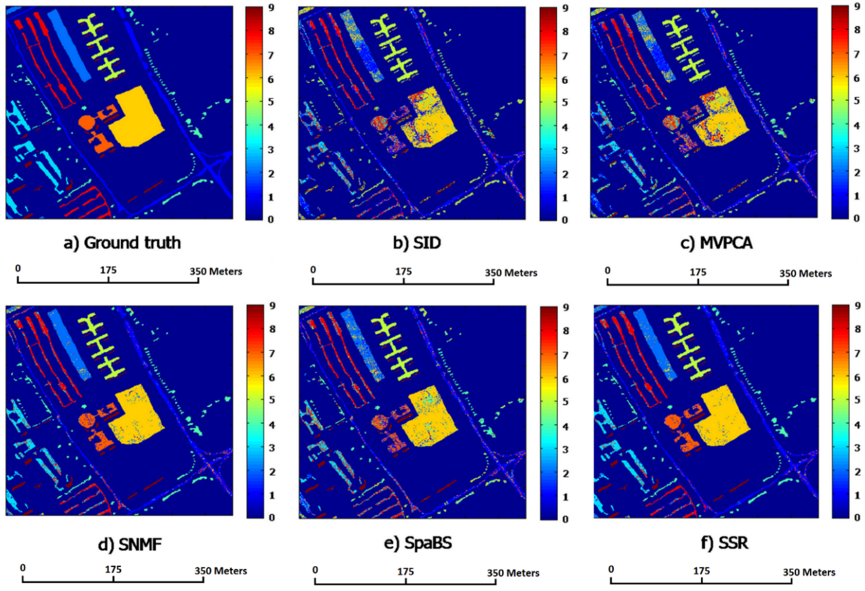
2. Methods

In this section, the Symmetric Sparse Representation (SSR) method is proposed. Section 2.1 describes the model of symmetric sparse representation on HSI bands, Section 2.2 presents the solution of the model and Section 2.3 gives the summary of the proposed method for band selection.

2.1. Symmetric Sparse Representation of HSI Bands

SNMF assumes that each band vector in HSI data can be sparsely represented by a coefficient vector in a basis or dictionary that is constituted with the aimed band subset. The SNMF simultaneously decomposes the HSI band matrix into the dictionary and a sparse coefficient matrix. SNMF was inspired from the idea of “blind source separation”, and the flexibility of SNMF renders that it is efficient in capturing the variances among different bands for selecting proper representative bands. However, the low-rank approximations of SNMF cannot provide reasonable explanations on the selected band subset. In contrast, the SSC based methods improve from subspace clustering, and state that each selected band is sampled from a defined subspace and it could be sparsely represented by all the other bands from the HSI data. The benefit of clustering and subspace assumptions gives the SSC an easy and interpretable band subset. Nevertheless, the binary assignments in the clustering reduce the flexibility of the SSC model and the result of clustering strongly depends on the heuristics of clustering centers. Therefore, we propose the Symmetric Sparse Representation (SSR) model to combine the virtue of SSC and the flexibility of SNMF.

The SSR model assumes that the selected bands are convex combinations of the original HSI bands and the total HSI bands are approximated in terms of convex combinations of the selected band subset. Consider all the HSI band vectors to constitute a band matrix $Y={\left\{y_j\right\}}_{j=1}^N\in R^{D\times N}$, where each band vector $y_j$in each column corresponds to a band point in the D-dimensional feature space, D is equal to the number of pixels in the image scene and N is the number of bands with $N\ll D$. Band selection is used to find the representative or exemplar bands from the original HSI band set, and accordingly SSR assumes that the HSI band matrix can be successfully reconstructed by the selected band vectors using a sparse coefficient matrix. The assumption formulates an equation of SNMF that the HSI band matrix can be simultaneously decomposed as the aimed band subset and the sparse coefficient matrix [36], shown in the following:

$$Y=ZA+E_1$$

(1)

where the matrix $Z\in R^{D\times k}$ is the dictionary matrix constituted with the selected band vectors, k is the size of band subset, $A={\left\{a_i\right\}}_{i=1}^N\in R^{k\times N}$ is the sparse coefficient matrix with $a_i\ge 0$ and $\left|a_i\right|=1$ and $E_1\in R^{D\times N}$ is the error term of all the band vectors. The constraint $a_i\ge 0$ ensures nonnegative coefficients to satisfy the reality of HSI band vectors. The constraint $\left|a_i\right|=1$ guarantees the probability that an arbitrary i-th band is represented by the selected bands is equal to 1. The error matrix $E_1$ mainly originates from approximation errors in the representation by the selected bands and Gaussian noises in all band vectors.

Meanwhile, the SSR assumes that all the HSI bands are sampled from a union of independent subspaces constituted from several bands, each representative band $z_j$ can then be approximately sparsely represented in the feature space spanned by all the bands [46],

$$z_j\approx Y{b}_j, b_{jj}=0$$

(2)

where $b_j$ is a sparse coefficient vector that shows the coordinates of $z_{j }$ in the feature space, having $b_j\ge 0, b_{jj}=0 \text{and}\left|b_j\right|=1.$ The constraint $b_j\ge 0$ ensures nonnegative coefficients to satisfy the reality of HSI band vectors. The constraint $b_{jj}=0$ is to eliminate a trivial solution that each selected band is simply a representation of itself. The constraint $\left|b_j\right|=1$ guarantees the probability that an and arbitrary selected band $z_j$ is represented by all the other band vectors is equal to 1. The positions of nonzero entries in $b_j$ denote the other bands from the same subspace (i.e., cluster) that the representative band $z_j$ belongs to. When stacking all the k selected bands together in the column format, the selected band vectors can be sparsely represented by the original band vectors,

$$Z=YB+E_2, \text{diag}\left(B\right)=0$$

(3)

where $B={\left\{b_j\right\}}_{j=1}^k\in R^{N\times k}$ is the sparse coefficient matrix, and $E_2\in R^{D\times k}$ is the error term that comes from the Gaussian noises in bands and approximation errors in the representation model. The constraint $\left(B\right)=0$ is to avoid a trivial solution that all the selected bands are self-represented by themselves. Nonzero entries in each column of B illustrate the band constituents of its subspace, and all the bands are concentrated into the k independent subspaces. Substituting the Equation (3) into Equation (1), the formulated Symmetric Sparse Representation (SSR) model for the HSI bands is the following:

$$Y=YBA+E, s.t., \{\begin{array}{c}{b}_j\ge 0,b_{jj}=0 and \left|b_j\right|=1, \forall j\in \left\{1,\mathrm{\cdot \cdot \cdot },k\right\} \\ a_i\ge 0 and \left|a_i\right|=1, \forall i\in \left\{1,\mathrm{\cdot \cdot \cdot },N\right\}\end{array}, 1<k<N$$

(4)

where $Y$is the band matrix constituted with all band column vectors, B and A are sparse coefficient matrices and are column stochastic, and the error term $E$ combines both errors in Equations (1) and (3) that come from noises in band vectors and approximation errors in the sparse representation models. Equation (4) integrates SNMF and SSC, and hence the SSR model has the features of flexibility and easy interpretation.

2.2. The Solution of SSR Model for Band Selection

The solution of Equation (4) can be transformed into the famous archetypal analysis problem [48] shown in Equation (5)

$$\underset{B,A}{\text{argmin}}Y-YB{A}_F^2, s.t., \{\begin{array}{c}{b}_j\ge 0,b_{jj}=0 and \left|b_j\right|=1, \forall j\in \left\{1,\mathrm{\cdot \cdot \cdot },k\right\} \\ a_i\ge 0 and \left|a_i\right|=1, \forall i\in \left\{1,\mathrm{\cdot \cdot \cdot },N\right\}\end{array}, 1<k<N$$

(5)

where ${||·||}_F$ is the Frobenious norm. Archetypal analysis assumes that archetypes are convex combinations of all band points and all band points are approximated in terms of convex combinations of archetypes [49]. Therefore, selecting a proper band subset is then explained as finding archetypes of the minimal convex hull of the high-dimensional band points [50]. The coefficient matrices B and A in Equation (5) are unknown, and that makes the un-convex optimization problem challenging to solve. Fortunately, the problem becomes convex with respect to one of the variables A or B when the other one is fixed. In this study, we utilize the block-coordinate descent scheme to achieve an optimal solution of problem Equation (5). First, the selected band subset $Z^{\left(0\right)}$ is initialized via the FurthestSum algorithm [51] and the initial sparse coefficient matrix $B^{\left(0\right)}$ is obtained via $Z^{\left(0\right)}=Y{B}^{\left(0\right)}$. The FurthestSum proceeds in the following three steps: (1) A subset $Z^{\left(0\right)}$ with k bands is randomly selected from the original band set; (2) for an arbitrary j-th random band $z_j^{\left(0\right)}\in Z^{\left(0\right)}$, a unique feature band vector ${\mathrm{z}}_j^{\text{'}\left(0\right)}$ that has maximal Euclidean distance with $z_j^{\left(0\right)}$ is chosen from the original band set; and (3) the random band ${\text{z}}_j^{\left(0\right)}$ is replaced by its corresponding feature band ${\mathrm{z}}_{\mathrm{j}}^{\text{'}\left(0\right)}$ and the $Z^{\left(0\right)}$ is renewed as the FurthestSum band subset. The careful selected initial band subset $Z^{\left(0\right)}$ from the FurthestSum scheme improves the convergence speed of optimization problem Equation (5) and lowers its risk in finding insignificant bands, especially to avoid selecting the too-close bands. After that, the block-coordinate descent scheme optimizes the variables B and A with iterative procedures and updates each variable at iteration t+1 using the following schemes [48]. When fixing the variable $B^{\left(t\right)}$ at the t-th iteration, each column $a_i^{\left(t+1\right)}$ in the variable A is optimized by minimizing the following quadratic program:

$$a_i^{\left(t+1\right)}=\text{argmin}||y_i-Z^{\left(t\right)}{a}_i^{\left(t\right)}{||}_2^2, s.t., a_i\ge 0 and \left|a_i\right|=1, \forall i\in \left\{1,\mathrm{\cdot \cdot \cdot },N\right\}$$

(6)

After the ergodic process of all columns, the variable $A^{\left(t+1\right)}$ at the t+1-th iteration is obtained. On the other hand, when fixing variable $A^{\left(t+1\right)}$, variable $B^{\left(t+1\right)}$ is estimated with the update scheme in each column $b_j$, where the $b_j$ at the t + 1 iteration is optimized with the quadratic program Equation (7):

$$\begin{array}{c}{b}_j^{\left(t+1\right)}=\text{argmin}||Y-Y{B}^{\left(t\right)}{A}^{\left(t+1\right)}+Y\left(b_j^{\left(t\right)}-b_j^{\left(t+1\right)}\right)a^j{||}_2^2\\ s.t., b_j\ge 0,b_{jj}=0 and \left|b_j\right|=1, \forall j\in \left\{1,\mathrm{\cdot \cdot \cdot },k\right\}\end{array}$$

(7)

where $b_j^{\left(t\right)}$ is the j-th column of variable $B^{\left(t\right)}$ at the t-th iteration, and $a^j$ is the j-th row of variable $A^{\left(t+1\right)}$ at the t+1 iteration. Variable $B^{\left(t+1\right)}$ at the t + 1-th iteration is estimated after the egrodic procedure of all its columns. The active-set algorithm [52] is utilized to solve the quadratic programs in Equations (6) and (7), and it implements an aggressive strategy that leverages the underlying sparsity feature of variables B and A. The above updates for $A^{\left(t+1\right)}$ and $B^{\left(t+1\right)}$ are repeated until satisfying the convergence conditions or the number of iterations exceeds the predefined maximal iteration number. The convergence condition is set as $||Y-Y{B}^{\left(t+1\right)}{A}^{\left(t+1\right)}{||}_{\infty }\le \mathsf{\epsilon }$, where $\mathsf{\epsilon }$ is the defined error tolerance for the residuals. The variables $A^{\left(t+1\right)}$ and $B^{\left(t+1\right)}$ at the stopping iteration are set as the optimal sparse coefficient matrices and the estimated band subset $\tilde{Z}$ is obtained via $\tilde{Z}=Y{B}^{\left(t+1\right)}$.

The achieved matrix $\tilde{Z}$ does not represent the real subset from HSI data because of approximation errors in Equation (4). Therefore, we select the real bands that are nearest to the estimated $\tilde{Z}$ from the original band collection to replace the estimated result. The index set $c={\left\{c_j\right\}}_{j=1}^k$ of the real band subset is obtained using the following optimization Equation (8)

$$c_j=\underset{i=1,\mathrm{\cdot \cdot \cdot },N}{\text{argmin}}{||{\tilde{z}}_j-y_i||}_2^2,\forall j\in \left\{1,\mathrm{\cdot \cdot \cdot },k\right\}$$

(8)

where ${\tilde{z}}_j$ is the j-th column of the estimated $\tilde{Z}$. The final band subset $\widehat{Z}$ is picked with the achieved index set c.

2.3. The Summary of SSR for Band Selection

The SSR method stands on two symmetric assumptions: the original band set is sparsely represented by the dictionary matrix of the selected band subset, and each band in the selected subset can be sparsely represented by all the original bands except itself. The SSR formulates band selection into the problem of archetypal analysis, and solves the problem with the block-coordinate descent scheme. Meanwhile, the SSR utilizes the FurthestSum algorithm to obtain a good initialization of band subset $Z^{\left(0\right)}$. The sparse coefficient matrices B and A are obtained when the convergence conditions satisfy or the number of iterations exceeds the maximal iteration number. Considering that the estimated band subset is not included in the original band set, the real bands that have smallest divergence with the estimated bands are selected from the original band collection and are set as candidates of the final band subset. The SSR method implements as follows:

(1)

Hyperspectral images are transformed from a data cube into a two-dimensional real band matrix $Y\in R^{D\times N}$, where D is the number of pixels and N is the number of bands.

(2)

With the predefined size k of the band subset, the SSR model represents the HSI bands with Equation (4), where B and A are the aimed sparse coefficient matrices.

(3)

The solution of SSR is reformulated into an archetypal analysis problem in Equation (5), and the block-coordinate descent algorithm is introduced to solve the problem. The algorithm is implemented as an iterative scheme and each column in A and B is updated via solving the quadratic program in Equations (6) and (7), respectively.

(4)

The variables A and B at the stopping iteration are set as the estimated matrices and the estimated band subset is obtained via $\tilde{Z}=YB$.

(5)

The band $y_i\in Y$ that is nearest to the estimated ${\widehat{Z}}_j\in \tilde{Z}$ using Equation (8) is set as one candidate of the final subset and the real band subset $\widehat{Z}$ is finally obtained.

The computational complexity of FurthestSum procedure is $O\left(DNk+Nk\text{log}N\right)$, where D is the number of pixels in the image scene, N is the number of HSI bands and k is the size of band subset. In Equation (6), each iteration in updating the column of variable A has the computational complexity less than $O\left(Dk+k^2\right)$, and thus the computational complexity in updating variables A at each iteration approaches $O\left(DNk+N{k}^2\right)$. Similarly, the computational complexity in updating variables B at each iteration is approximately $O\left(D{k}^2+k{N}^2\right)$. Therefore, the total complexity of the SSR method for band selection is less than $O\left(Nk\left(D+\text{log}N\right)+kt\left(D+N\right)\left(k+N\right)\right)$ and it approaches $O\left(Nk\left(D+\text{log}N\right)+ktDN\right)$ because $\mathrm{k}\ll \mathrm{N}\ll \mathrm{D}.$

3. Experiments

In this section, three groups of experiments on two HSI datasets are designed to testify the SSR method for band selection. Section 3.1 describes the information of two HSI datasets. Section 3.2 lists detailed results from the three groups of experiments.

3.1. Descriptions of Two HSI Datasets

The Indian Pines dataset was collected by NASA on 12 June 1992 using the AVIRIS sensor from JPL. It has 20 m spatial resolution and 10 nm spectral resolution, covering a spectrum range of 200–2400 nm. A subset of the image scene of size 145 × 145 pixels is implemented in the experiment and it covers an area of 6 miles west of West Lafayette, Indiana. The dataset was pre-processed with radiometric corrections and bad band removal, and 200 bands were left with calibrated data values proportional to radiances. Sixteen classes of ground objects exist in the image scene (Figure 1), and the ground truth for both training and testing samples in each class is listed in

Table 1. The ground truth of training and testing samples in each class for Indian Pines dataset.

Class		Sample
Label	Name	Train	Test
1	Alfalfa	9	37
2	Corn-notill	286	1142
3	Corn-min	166	664
4	Corn	47	190
5	Grass/Pasture	97	386
6	Grass/Trees	146	584
7	Grass/pasture-mowed	6	22
8	Hay-windowed	96	382
9	Oats	4	16
10	Soybeans-notill	194	778
11	Soybeans-min	491	1964
12	Soybeans-clean	119	474
13	Wheat	41	164
14	Woods	253	1012
15	Bldg-Grass-Tree Drives	77	309
16	Stone-Steel towers	19	74
Total		2051	8198

.

The Pavia University (PaviaU) dataset was obtained from ROSIS sensor having 1.3 m spatial resolutions and 115 bands. After removing low SNR bands, the remaining 103 bands were utilized in the following experiments. A smaller subset of the larger dataset shown in Figure 2 contains 350 × 340 pixels and covers an area of Pavia University. The image scene has nine classes of ground objects, including shadows, and the ground truth information of training and testing samples in each class is listed in

Table 2. The ground truth of training and testing samples in each class for PaviaU dataset.

Class		Sample
Label	Name	Train	Test
1	Asphalt	839	3356
2	Meadows	437	1748
3	Gravel	420	1679
4	Trees	310	1240
5	Painted metal sheets	269	1076
6	Bare Soil	1006	4023
7	Bitumen	266	1064
8	Self-Blocking Bricks	469	1878
9	Shadows	186	743
Total		4202	16087

.

3.2. Experimental Results

In the following, we design three groups of experiments on both HSI datasets to explore the performance of the proposed method. Four state-of-the-art methods are utilized to make holistic comparisons with the SSR, including SID [18], MVPCA [21], SNMF [36] and SpaBS [35] methods. The first experiment quantifies the band selection performance of SSR and compares the results with those of the four other methods. The second experiment compares classification accuracies of SSR and the four other methods. Three popular classifiers are adopted in the experiment, Support Vector Machine (SVM) [53], K-Nearest Neighbor (KNN) [54] and Random Forest (RF) [55] classifiers. We quantify classification accuracies using Overall Classification Accuracy (OCA) and Average Classification Accuracy (ACA). The SVM classifier is implemented in the LIBSVM software package using the Radial Basis Function (RBF) kernel function [56] and the variance parameter and penalization factor in the SVM are estimated via cross-validation. The KNN classifier works with the Euclidean distance and the RF classifier is implemented in the “randomforest” package using default parameters [57]. The third experiment compares the computational complexity and computational times of all five methods. The following results, without specific clarifications, are the average results of ten different and independent experiments.

(1)

Quantitative evaluation of the SSR band subset. The experiment investigates the band selection performance of SSR before classification. We implement three quantitative measures, the Average Information Entropy (AIE), the Average Correlation Coefficient (ACC) and the Average Relative Entropy (ARE) (also called Average Kullback–Leibler Divergence, AKLD), to estimate the richness of spectrum information, the intra-band correlations and the intra-class separabilities of the selected band subset, respectively. The reason for the three quantitative measures is that we argue that a proper band subset should have higher information amount, low intra-band correlations and high intra-class separabilities. In the experiment, we manually choose the parameter k and then set them as the dimensions of band subsets from all five methods. The k in Indian Pines dataset is 12 and that of PaviaU dataset is 10. In the SNMF method, the parameter α controls the entry size of dictionary matrix and the parameter γ determines the sparseness of coefficient matrix. Using cross-validation, the α and γ of SNMF on Indian Pines dataset are chosen as 3.0 and 0.05, respectively, and the α and γ on PaviaU dataset are 4.0 and 0.001, respectively. The iteration time t for the learning dictionary in SpaBS is manually set as 5 for both HSI datasets.

Table 3. Contrast in quantitative evaluation of band subsets from all five methods on both datasets.

HSI Datasets	Quantitative Evaluation	Band Selection Methods
		SID	MVPCA	SNMF	SPABS	SSR
Indian Pines (k = 12)	AIE	9.74	9.72	10.53	9.52	9.85
	ACC	0.91	0.84	0.25	0.56	0.21
	ARE	15.51	16.64	18.39	35.63	36.74
PaviaU (k = 10)	AIE	10.80	10.86	11.25	10.84	11.37
	ACC	0.95	0.97	0.58	0.94	0.57
	ARE	0.46	0.49	1.65	0.52	1.97

compares quantitative evaluation results of SSR and the four other methods on both datasets. For the Indian Pines dataset, SSR has the highest ARE and the lowest ACC, whereas SNMF has the highest AIE. The AIE of SSR is lower than that of SNMF but it clearly outperforms SID, MVPCA and SpaBS. The SID and MVPCA behave worse when compared with the three other methods. For the PaviaU dataset, the SSR outperforms the four other methods in all three quantitative measures.

(2)

Classification performance of SSR. This experiment makes holistic evaluations in classification performance of SSR by varying the size of band subset k. The classification accuracies are quantified with the OCA and ACA and the results are averaged from ten independent experiments. In the experiment, the sizes of band subset k in Indian Pines and PaviaU datasets change from 5 to 45. The neighborhood size in the KNN classifier and the threshold of total distortion in the SVM classifier are set as 3 and 0.01 respectively. Using cross-validation, the α and γ in SNMF of PaviaU dataset are estimated as 3.0 and 0.1, respectively, and the α and γ in PaviaU are chosen as 4.0 and 1.5, respectively. Other parameters unmentioned are the same as their counterparts in the above experiments.

Figure 3 plots the OCAs of original HSI band sets and the band subsets of all five methods using SVM, KNN and RF classifiers on both datasets. The reason for omitting the ACA plots is the similarities with those of OCAs. All the plots from Figure 3a to Figure 3f rise from a small value and the changes become slow after a certain threshold, for both datasets and all three classifiers. The SID behaves worst among all the plots, regardless of classifier or HSI dataset. This coincides with the observations in Experiment (1). From all six figures, the OCA plots from SSR clearly surpass those of the four other methods, including SID, SpaBS, MVPCA and SNMF. When increasing the size of k, after a certain value, the SSR band subsets behave better than the original band sets in relation to OCAs. In contrast, the plots of the four other methods are inferior to those of the original band sets, whatever the size of k.

Moreover, we compare classification accuracies ACAs and OCAs from all five methods when the parameters of band subset size k equal those of Experiment (1). The contrast in ACAs and OCAs from all five methods is illustrated in

Table 4. Classification accuracies of all five methods with a certain k for both datasets.

HSI Datasets	Classifiers		Band Selection Methods (%)
			SID	MVPCA	SNMF	SPABS	SSR
Indian Pines (k = 12)	SVM	ACA	30.76	48.97	70.79	58.12	71.56
		OCA	45.43	58.53	77.26	67.64	77.62
	KNN	ACA	29.24	41.69	65.38	44.96	71.29
		OCA	36.11	46.00	71.96	52.39	71.74
	RF	ACA	38.35	47.55	65.83	59.34	65.07
		OCA	52.44	59.66	74.23	72.54	75.79
PaviaU (k = 10)	SVM	ACA	50.06	55.72	88.50	71.61	91.37
		OCA	54.79	59.56	88.62	72.03	91.52
	KNN	ACA	43.98	48.88	84.43	63.86	86.23
		OCA	44.09	48.98	85.24	63.90	85.69
	RF	ACA	52.58	58.32	87.75	71.78	89.46
		OCA	55.20	60.25	87.66	72.33	89.25

, and Figure 4 and Figure 5 show the classification maps of all methods on both datasets using the SVM classifier. The results from the three classifiers show that SSR performs better than the four other methods and further verify the above conclusions.

(3)

Computational performance of SSR. This experiment explores the computational performance of SSR against the four other methods.

Table 5. The contrast in computational complexity of SSR and the four other methods.

Computational complexity	Band Selection Methods
	SID	MVPCA	SNMF	SpaBS	SSR
	O (N2D)	O (kN + D2)	O (DNkt)	O (2D2Nt + DNtK2)	O(Nk (D + logN) + ktDN)

lists the computational complexity of all five methods, where parameter D is the number of pixels in the image scene, k is the size of band subset, N is the number of bands (i.e., the size of original band set), t is the iteration time, and K is the sparsity level in the SpaBS method. In the table, we can see that SpaBS has the highest computational complexity among all the methods and SSR has lower computational complexity.

Furthermore, we compare the computational times of the five methods by changing the size of band subset from 10 to 50 with a step interval of 10. The experiment is carried out using a Windows 7 computer with Intel i5-4570 Quad Core Processor and 8 GB of RAM. SSR and the four other methods are implemented in Matlab 2014a. The results in

Table 6. Computational times of all five methods on both HSI datasets.

Datasets	Size of Subset k	Computational Times (s)
		SID	MVPCA	SNMF	SpaBS	SSR
Indian Pines	k = 10	4.83	5.93	7.99	492.57	5.02
	k = 20	6.14	8.59	9.28	550.83	8.08
	k = 30	7.19	14.69	17.27	638.78	11.44
	k = 40	8.45	20.41	22.51	710.40	16.54
	k = 50	9.03	44.21	49.39	832.50	20.34
PaviaU	k = 10	15.29	27.53	32.59	1728.66	21.49
	k = 20	18.78	43.14	51.68	2237.46	26.55
	k = 30	22.54	59.20	70.22	3141.39	33.88
	k = 40	24.48	81.73	89.54	4277.56	40.37
	k = 50	27.54	102.42	121.77	5429.08	45.62

show that all five methods have the computational complexity increase with the rising k. Among all the methods, SID has the fastest computational speeds and takes the shortest time at the same parameter k and on the same HSI dataset. The SSR has shorter computational times than those of MVPCA, SNMF and SpaBS, and it has the second fastest computational speeds. The computational times of SNMF are longer than those of MVPCA but clearly outperform those of SpaBS. SpaBS performs worst among all the methods with respect to computational speeds. The computational speeds in descending order are the following: SID, SSR, MVPCA, SNMF and SpaBS.

4. Discussions

This section discusses the performances of SSR compared to the four other state-of-the-art methods from Section 3.2 in detail. Three experiments have been designed using Indian Pines and PaviaU datasets to compare the SSR method to SID, MVPCA, SpaBS and SNMF. Three quantitative measures, AIE, ACC and ARE, show that SSR outperforms the four other methods. SSR assumes that the selected bands and the original HSI bands are symmetrically sparsely represented by each other. 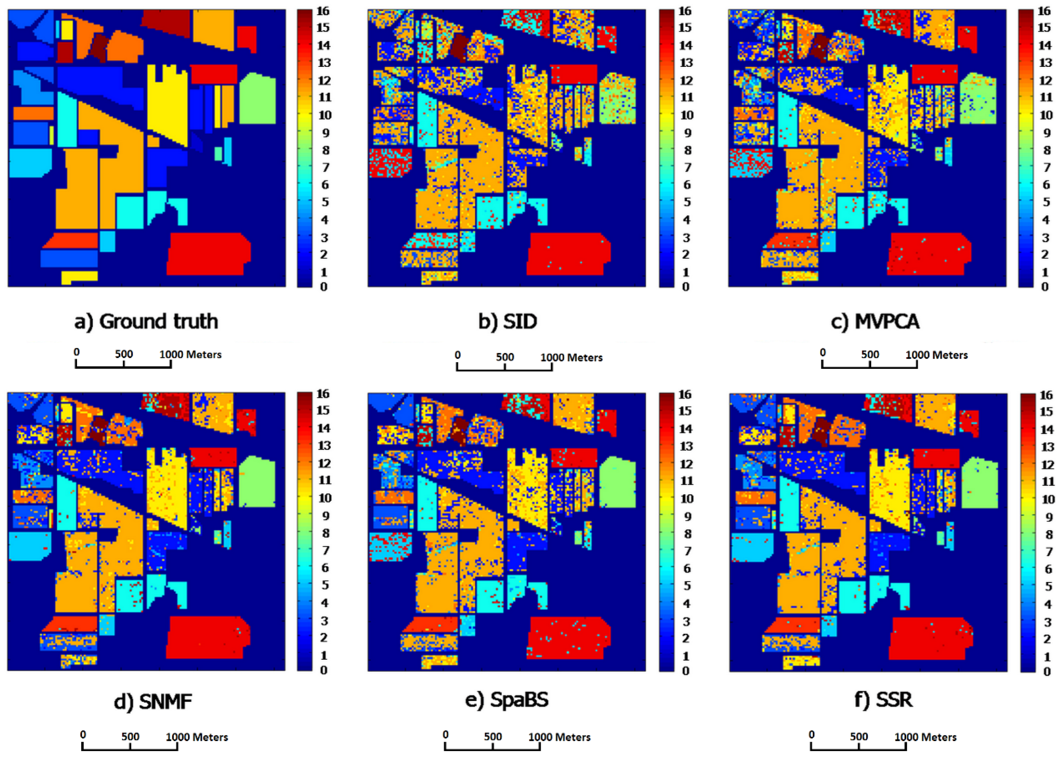The two sparse representation assumptions interpret band selection as finding archetypes (i.e., representative corners) of the minimal convex hull containing the HSI band points. Hence, the SSR subset has high information amount, high intra-class separabilities and low intra-band correlations. The SSR satisfies the requirements of band subset selection and is more appropriate for band selection than the four other methods, especially SID and MVPCA.

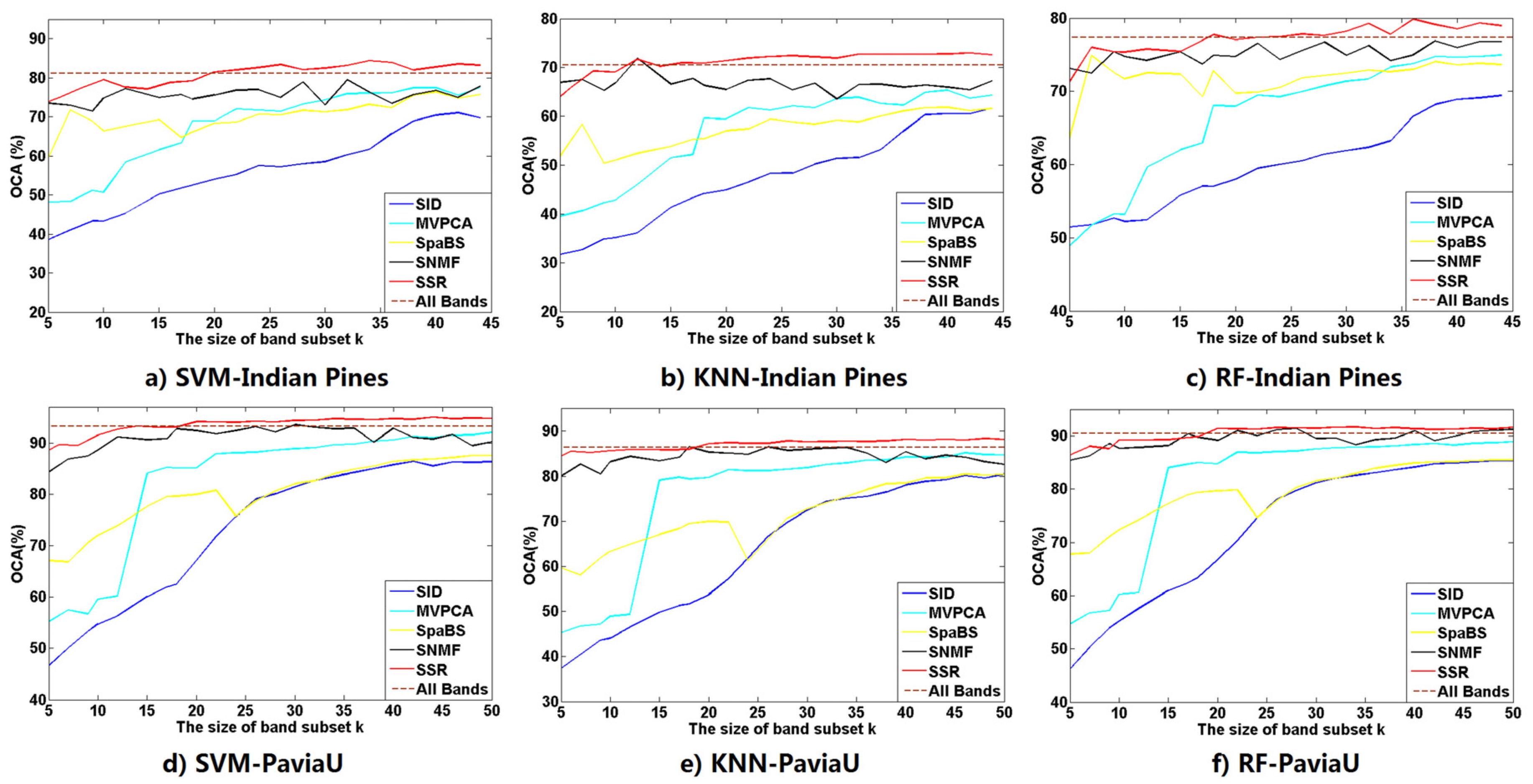
The classification and computation experiments compare classification and computational performances of the SSR band subset with those of the four other methods. The SID has the fastest computational speeds whereas its band subset obtains worst ACAs and OCAs. The fastest speed of SID results from its lowest computational complexity in computing the diagonal elements of its similarity matrix. The SpaBS has better classification accuracies, ACAs and OCAs, than SID but it costs the longest computational time. The reason for that is the extremely high complexity of dictionary learning using K-SVD algorithm. The slower computational speed of MVPCA than SSR results from the lower computation in principal component analysis transformation. The SSR behaves best among all five methods in classification accuracies OCAs and ACAs while it takes the second shortest computational times. Moreover, compared with the four other methods, the SSR band subsets exclusively achieve better OCAs than the original band sets on both HSI datasets, when having a larger size k than a certain value. This implies that SSR could select a proper band subset and could help solve the “curse of dimensionality” problem in HSI classification.

However, we have to clarify that SSR requires no more parameter setting work, except the size of band subset k. We did manually estimate the size of band subset and did not carefully investigate a proper size for the selected bands. Aside from the size problem of a band subset, SSR is the best candidate among all five methods for selecting a proper band subset from HSI bands because of its comprehensive performances in classification and computation. The reason we did not explore setting a proper size for the SSR method is that different estimation criteria in various methods renders it confusing, and even difficult, to estimate a unique and proper size. The unification of all current estimation methods of band subset size is then the first significant problem we aim to solve in future work. One big possible uncertainty of SSR in band selection for HSI classification is the effect from atmospheric calibration on both HSI datasets. We decided to make no atmospheric correction in this manuscript to facilitate comparison with other methods. Nevertheless, atmospheric calibration does make clear effects in classification results of HSI datasets. Therefore, the second aim of our future work is to carefully analyze the effects of atmospheric calibration on the classification performance of SSR and continue to ameliorate classification results of the SSR band subset in realistic classification applications.

5. Conclusions

In this study, we propose a SSR method to study the band selection problem of HSI dataset. The SSR method has the following two symmetric assumptions: that the HSI bands can be reconstructed by the selected bands with a sparse coefficient matrix and the selected bands can be sparsely represented in the feature space spanned by the HSI bands. The SSR method selects the representative bands by finding archetypes of the minimal convex hull containing the HSI band points. The SSR method estimates the representative bands by solving an optimization program with the block-coordinate descent scheme and the final representative bands are obtained by picking the real counterpart that has the smallest differences with each element in the estimated $\tilde{Z}$. Three groups of experiments on Indian Pines and PaviaU datasets were carefully designed to test the SSR method and the results are compared with those of four state-of-the-art methods and the original band sets. SSR outperforms the four other methods in three quantitative measures, AIE, ACC and ARE, and has the best classification accuracies, ACAs and OCAs. Moreover, the SSR subset could obtain better classification accuracies than the original band set and then could successfully deal with the “curse of dimensionality” problem in HSI classification. Besides, the contrast in computational times illustrate that SSR has the second shortest computational times among all five methods. Therefore, SSR is a good alternative for band selection on HSI dataset in realistic classification applications.

References

1. Giardino, C.; Bresciani, M.; Valentini, E.; Gasperini, L.; Bolpagni, R.; Brando, V.E. Airborne hyperspectral data to assess suspended particulate matter and aquatic vegetation in a shallow and turbid lake. Remote Sens. Environ. 2015, 157, 48–57. [Google Scholar] [CrossRef]
2. Bell, T.W.; Cavanaugh, K.C.; Siegel, D.A. Remote monitoring of giant kelp biomass and physiological condition: An evaluation of the potential for the Hyperspectral Infrared Imager (HyspIRI) mission. Remote Sens. Environ. 2015, 167, 218–228. [Google Scholar] [CrossRef]
3. Bareth, G.; Aasen, H.; Bendig, J.; Gnyp, M.L.; Bolten, A.; Jung, A.; Michels, R.; Soukkamäki, J. Low-weight and uav-based hyperspectral full-frame cameras for monitoring crops: Spectral comparison with portable spectroradiometer measurements. Photogramm. Fernerkund. Geoinf. 2015, 1, 69–79. [Google Scholar] [CrossRef]
4. Liang, L.; Di, L.; Zhang, L.; Deng, M.; Qin, Z.; Zhao, S.; Lin, H. Estimation of crop lai using hyperspectral vegetation indices and a hybrid inversion method. Remote Sens. Environ. 2015, 165, 123–134. [Google Scholar] [CrossRef]
5. Cui, J.; Yan, B.; Dong, X.; Zhang, S.; Zhang, J.; Tian, F.; Wang, R. Temperature and emissivity separation and mineral mapping based on airborne tasi hyperspectral thermal infrared data. Int. J. Appl. Earth Obs. Geoinf. 2015, 40, 19–28. [Google Scholar] [CrossRef]
6. Zabcic, N.; Rivard, B.; Ong, C.; Mueller, A. Using airborne hyperspectral data to characterize the surface ph and mineralogy of pyrite mine tailings. Int. J. Appl. Earth Obs. Geoinf. 2014, 32, 152–162. [Google Scholar] [CrossRef]
7. Donoho, D.L. High-dimensional data analysis: The curses and blessings of dimensionality. In Proceedings of the 2000 American Math Society Math Challenges of the 21st Century, Los Angeles, CA, USA, 6–11 August 2000; pp. 1–32.
8. Melgani, F.; Bruzzone, L. Classification of hyperspectral remote sensing images with support vector machines. IEEE Trans. Geosci. Remote Sens. 2004, 42, 1778–1790. [Google Scholar] [CrossRef]
9. Camps-Valls, G.; Marsheva, T.V.B.; Zhou, D. Semi-supervised graph-based hyperspectral image classification. IEEE Trans. Geosci. Remote Sens. 2007, 45, 3044–3054. [Google Scholar] [CrossRef]
10. Zhang, L.; Zhang, L.; Tao, D.; Huang, X. Tensor discriminative locality alignment for hyperspectral image spectral–spatial feature extraction. IEEE Trans. Geosci. Remote Sens. 2013, 51, 242–256. [Google Scholar] [CrossRef]
11. Du, B.; Zhang, L. Random-selection-based anomaly detector for hyperspectral imagery. IEEE Trans. Geosci. Remote Sens. 2011, 49, 1578–1589. [Google Scholar] [CrossRef]
12. Tong, Q.X.; Zhang, B.; Zheng, L.-F. Hyperspectral Remote Sensing: Principle, Technology and Application; Higher Education Press: Beijing, China, 2006. [Google Scholar]
13. Plaza, A.; Benediktsson, J.A.; Boardman, J.W.; Brazile, J.; Bruzzone, L.; Camps-Valls, G.; Chanussot, J.; Fauvel, M.; Gamba, P.; Gualtieri, A. Recent advances in techniques for hyperspectral image processing. Remote Sens. Environ. 2009, 113, S110–S122. [Google Scholar] [CrossRef]
14. Zhang, L.; Zhang, L.; Tao, D.; Huang, X. On combining multiple features for hyperspectral remote sensing image classification. IEEE Trans. Geosci. Remote Sens. 2012, 50, 879–893. [Google Scholar] [CrossRef]
15. Sun, W.; Halevy, A.; Benedetto, J.J.; Czaja, W.; Li, W.; Liu, C.; Shi, B.; Wang, R. Nonlinear dimensionality reduction via the ENH-LTSA method for hyperspectral image classification. IEEE J. Sel. Top. Appl. Earth Obs. Remote Sens. 2014, 7, 375–388. [Google Scholar] [CrossRef]
16. Bajcsy, P.; Groves, P. Methodology for hyperspectral band selection. Photogramm. Eng. Remote Sens. 2004, 70, 793–802. [Google Scholar] [CrossRef]
17. Arzuaga-Cruz, E.; Jimenez-Rodriguez, L.O.; Velez-Reyes, M. Unsupervised feature extraction and band subset selection techniques based on relative entropy criteria for hyperspectral data analysis. Proc. SPIE 2003, 5093. [Google Scholar] [CrossRef]
18. Keshava, N. Distance metrics and band selection in hyperspectral processing with applications to material identification and spectral libraries. IEEE Trans. Geosc. Remote Sens. 2004, 42, 1552–1565. [Google Scholar] [CrossRef]
19. Mausel, P.; Kramber, W.; Lee, J. Optimum band selection for supervised classification of multispectral data. Photogramm. Eng. Remote Sens. 1990, 56, 55–60. [Google Scholar]
20. Guo, B.; Gunn, S.R.; Damper, R.; Nelson, J. Band selection for hyperspectral image classification using mutual information. IEEE Geosci. Remote Sens. Lett. 2006, 3, 522–526. [Google Scholar] [CrossRef]
21. Chang, C.-I.; Du, Q.; Sun, T.-L.; Althouse, M.L. A joint band prioritization and band-decorrelation approach to band selection for hyperspectral image classification. IEEE Trans. Geosci. Remote Sens. 1999, 37, 2631–2641. [Google Scholar] [CrossRef]
22. Shi, Q.; Zhang, L.; Du, B. Semisupervised discriminative locally enhanced alignment for hyperspectral image classification. IEEE Trans. Geosci. Remote Sens. 2013, 51, 4800–4815. [Google Scholar] [CrossRef]
23. Wang, C.; Gong, M.; Zhang, M.; Chan, Y. Unsupervised hyperspectral image band selection via column subset selection. IEEE Geosci. Remote Sens. Lett. 2015, 12, 1411–1415. [Google Scholar] [CrossRef]
24. Yang, H.; Du, Q.; Chen, G. Particle swarm optimization-based hyperspectral dimensionality reduction for urban land cover classification. IEEE J. Sel. Top. Appl. Earth Obs. Remote Sens. 2012, 5, 544–554. [Google Scholar] [CrossRef]
25. Chang, Y.L.; Fang, J.P.; Benediktsson, J.A.; Chang, L.Y.; Ren, H.; Chen, K.S. Band selection for hyperspectral images based on parallel particle swarm optimization schemes. In Proceedings of the 2009 IEEE International Geoscience and Remote Sensing Symposium, Cape Town, South Africa, 12–17 July 2009.
26. Shen, J.; Wang, C.; Wang, R.; Huang, F.; Fan, C.; Xu, L. A band selection method for hyperspectral image classification based on improved particle swarm optimization. Int. J. Signal Process. Image Process. Pattern Recognit. 2015, 8, 325–338. [Google Scholar] [CrossRef]
27. Tang, C.; Wu, Y.; Huang, J. Band selection of hyperspectral chlorophyll-a concentration inversion based on parallel ant colony algorithm. Appl. Mech. Mater. 2014, 675, 1158–1162. [Google Scholar] [CrossRef]
28. Gao, J.; Du, Q.; Gao, L.; Sun, X.; Zhang, B. Ant colony optimization-based supervised and unsupervised band selections for hyperspectral urban data classification. J. Appl. Remote Sens. 2014, 8. [Google Scholar] [CrossRef]
29. Xia, W.; Wang, B.; Zhang, L. Band selection for hyperspectral imagery: A new approach based on complex networks. IEEE Geosci. Remote Sens. Lett. 2013, 10, 1229–1233. [Google Scholar] [CrossRef]
30. Xia, W.; Dong, Z.; Pu, H.; Wang, B.; Zhang, L. Network topology analysis: A new method for band selection. In Proceedings of the 2012 IEEE International Geoscience and Remote Sensing Symposium (IGARSS), Munich, Germany, 22–27 July 2012; pp. 3062–3065.
31. Chang, C.-I.; Liu, K.-H. Progressive band selection of spectral unmixing for hyperspectral imagery. IEEE Trans. Geosci. Remote Sens. 2014, 52, 2002–2017. [Google Scholar] [CrossRef]
32. Sun, K.; Geng, X.; Ji, L. A band selection approach for small target detection based on cem. Int. J. Remote Sens. 2014, 35, 4589–4600. [Google Scholar] [CrossRef]
33. Feng, J.; Jiao, L.; Zhang, X.; Sun, T. Hyperspectral band selection based on trivariate mutual information and clonal selection. IEEE Trans. Geosci. Remote Sens. 2014, 52, 4092–4105. [Google Scholar] [CrossRef]
34. Du, Q.; Bioucas-Dias, J.M.; Plaza, A. Hyperspectral band selection using a collaborative sparse model. In Proceedings of the 2012 IEEE International Geoscience and Remote Sensing Symposium (IGARSS), Munich, Germany, 22–27 July 2012; pp. 3054–3057.
35. Li, S.; Qi, H. Sparse representation based band selection for hyperspectral images. In Proceedings of the 18th IEEE International Conference on in Image Processing (ICIP), Brussels, Belgium, 11–14 September 2011; pp. 2693–2696.
36. Li, J.-M.; Qian, Y.-T. Clustering-based hyperspectral band selection using sparse nonnegative matrix factorization. J. Zhejiang Univ. Sci. C 2011, 12, 542–549. [Google Scholar] [CrossRef]
37. Willett, R.M.; Duarte, M.F.; Davenport, M.; Baraniuk, R.G. Sparsity and structure in hyperspectral imaging: Sensing, reconstruction, and target detection. IEEE Signal Process. Mag. 2014, 31, 116–126. [Google Scholar] [CrossRef]
38. Davenport, M.A.; Duarte, M.F. Introduction to compressed sensing. Electr. Eng. 2011, 93, 1–68. [Google Scholar]
39. Sun, W.; Li, W.; Li, J.; Lai, Y.M. Band selection using sparse nonnegative matrix factorization with the thresholded earth’s mover distance for hyperspectral imagery classification. Earth Sci. Inform. 2015, 8, 907–918. [Google Scholar] [CrossRef]
40. Xiao, Z.; Bourennane, S. Constrained nonnegative matrix factorization and hyperspectral image dimensionality reduction. Remote Sens. Lett. 2014, 5, 46–54. [Google Scholar] [CrossRef]
41. Chepushtanova, S.; Gittins, C.; Kirby, M. Band selection in hyperspectral imagery using sparse support vector machines. Proc. SPIE 2014, 9088. [Google Scholar] [CrossRef]
42. Geng, X.; Sun, K.; Ji, L. Band selection for target detection in hyperspectral imagery using sparse cem. Remote Sens. Lett. 2014, 5, 1022–1031. [Google Scholar] [CrossRef]
43. Zhang, Q.; Tian, Y.; Yang, Y.; Pan, C. Automatic spatial–spectral feature selection for hyperspectral image via discriminative sparse multimodal learning. IEEE Trans. Geosci. Remote Sens. 2015, 53, 261–279. [Google Scholar] [CrossRef]
44. Yuan, Y.; Zhu, G.; Wang, Q. Hyperspectral band selection by multitask sparsity pursuit. IEEE Trans. Geosci. Remote Sens. 2015, 53, 631–644. [Google Scholar] [CrossRef]
45. Sun, K.; Geng, X.; Ji, L. A new sparsity-based band selection method for target detection of hyperspectral image. IEEE Geosci. Remote Sens. Lett. 2015, 12, 329–333. [Google Scholar]
46. Sun, W.; Zhang, L.; Du, B.; Li, W.; Lai, M.Y. Band selection using improved sparse subspace clustering for hyperspectral imagery classification. IEEE J. Sel. Top. Appl. Earth Obs. Remote Sens. 2015, 8, 1–14. [Google Scholar] [CrossRef]
47. Mørup, M.; Hansen, L.K. Archetypal analysis for machine learning. In Proceedings of the 2010 IEEE International Workshop on the Machine Learning for Signal Processing (MLSP), Kittilä, Finland, 29 August–1 September 2010; pp. 172–177.
48. Cutler, A.; Breiman, L. Archetypal analysis. Technometrics 1994, 36, 338–347. [Google Scholar] [CrossRef]
49. Bauckhage, C. A Note on Archetypal Analysis and the Approximation of Convex Hulls. Available online: http://arxiv.org/pdf/1410.0642v1.pdf (accessed on 19 November 2015).
50. Chen, Y.; Mairal, J.; Harchaoui, Z. Fast and robust archetypal analysis for representation learning. In Proceedings of the 2014 IEEE Conference on Computer Vision and Pattern Recognition (CVPR), Columbus, OH, USA, 24–27 June 2014; pp. 1478–1485.
51. Mørup, M.; Hansen, L.K. Archetypal analysis for machine learning and data mining. Neurocomputing 2012, 80, 54–63. [Google Scholar] [CrossRef]
52. Nocedal, J.; Wright, S. Numerical Optimization; Springer Science & Business Media: Medford, MA, USA, 2006. [Google Scholar]
53. Steinwart, I.; Christmann, A. Support Vector Machines; Springer Verlag: Berlin, Germany, 2008. [Google Scholar]
54. Cover, T.; Hart, P. Nearest neighbor pattern classification. IEEE Trans. Inf. Theory 1967, 13, 21–27. [Google Scholar] [CrossRef]
55. Liaw, A.; Wiener, M. Classification and regression by random forest. R News 2002, 2, 18–22. [Google Scholar]
56. Chang, C.C.; Lin, C.J. Libsvm: A library for support vector machines. ACM Trans. Intell. Syst. Technol. 2011, 2, 27–65. [Google Scholar] [CrossRef]
57. Breiman, L. Randomforest: Breiman and Cutler’s Random Forests for Classification and Regression, URL R Package Version. 2006. Available online: http://stat-www.berkeley.edu/users/breiman/RandomForests (accessed on 19 November 2015).
Figure 1. The image of Indian Pines dataset.
Remotesensing 08 00238 g001
Figure 2. The image of Pavia dataset.
Remotesensing 08 00238 g002
Figure 3. The OCA plots from SVM, KNN and RF classifiers on Indian Pines and PaviaU datasets. (a) SVM-Indian Pines; (b) KNN-Indian Pines; (c) RF-Indian Pines; (d) SVM-PaviaU; (e) KNN-PaviaU; and (f) RF-PaviaU
Remotesensing 08 00238 g003
Figure 4. Classification maps of all five methods on Indian Pines dataset using the SVM classifier. (a) Ground truth; (b) SID; (c) MVPCA; (d) SNMF; (e) SpaBS; and (f) SSR.
Remotesensing 08 00238 g004
Figure 5. Classification maps of all five methods on PaviaU dataset using the SVM classifier. (a) Ground truth; (b) SID; (c) MVPCA; (d) SNMF; (e) SpaBS; and (f) SSR.
Remotesensing 08 00238 g005