Interseismic Deformation of the Altyn Tagh Fault Determined by Interferometric Synthetic Aperture Radar (InSAR) Measurements

Abstract

The Altyn Tagh Fault (ATF) is one of the major left-lateral strike-slip faults in the northeastern area of the Tibetan Plateau. In this study, the interseismic deformation across the ATF at 85°E was measured using 216 interferograms from 33 ENVISAT advanced synthetic aperture radar images on a descending track acquired from 2003 to 2010, and 66 interferograms from 15 advanced synthetic aperture radar images on an ascending track acquired from 2005 to 2010. To retrieve the pattern of interseismic strain accumulation, a global atmospheric model (ERA-Interim) provided by the European Center for Medium Range Weather Forecast and a global network orbital correction approach were applied to remove atmospheric effects and the long-wavelength orbital errors in the interferograms. Then, the interferometric synthetic aperture radar (InSAR) time series with atmospheric estimation model was used to obtain a deformation rate map for the ATF. Based on the InSAR velocity map, the regional strain rates field was calculated for the first time using the multi-scale wavelet method. The strain accumulation is strongly focused on the ATF with the maximum strain rate of 12.4 × 10⁻⁸/year. We also show that high-resolution 2-D strain rates field can be calculated from InSAR alone, even without GPS data. Using a simple half-space elastic screw dislocation model, the slip-rate and locking depth were estimated with both ascending and descending surface velocity measurements. The joint inversion results are consistent with a left-lateral slip rate of 8.0 ± 0.7 mm/year on the ATF and a locking depth of 14.5 ± 3 km, which is in agreement with previous results from GPS surveys and ERS InSAR results. Our results support the dynamic models of Asian deformation requiring low fault slip rate.

1. Introduction

The ongoing active continental collision between the Indian and Eurasian plates has created the massive topography of the Tibetan Plateau over the last 50 million years. The tectonic processes underlying this region are still not completely understood and a number of models have been proposed to explain the dynamics of the area [1,2,3,4]. The active Altyn Tagh Fault (ATF) is a distinctive feature of Tibetan geography, inscribing a fairly linear trace over 1500 km across northern Tibet (Figure 1), separating the high plateau in the south from the low Tarim Basin in the north. The Tibetan Plateau south of the ATF has an average elevation of ~4000 m, whereas the northern Tarim Basin has an average elevation of only ~1000 m. The ATF begins in the west at the Pamir Mountains and ends in the east near the Qilian Mountains. It is generally accepted that the ATF is divided into three segments, the west, middle, and east, between 84°E and 94°E [5]. It is a major tectonic element in the Cenozoic Indo–Asian collision zone [6] that defines the northern margin of the Tibetan Plateau. It plays a key role in identifying the Tibet deformation patterns and its slip rates have constituted an important constraint for deriving the velocity field of East Asia [7]. Some studies argued that the ATF might accommodate as much as one-third of the overall convergence between India and Siberia [7]. Zhang et al. [8] derived the velocity field of the present day tectonic deformation in the Tibetan Plateau using 553 GPS observations. The velocity distribution suggested that the relative movement between the Indian and Eurasian plates was adjusted and absorbed by crustal shortening and internal strike-slip shearing in the Tibetan Plateau. In particular, the Himalaya Mountains absorbed 44%–53% of the total shortening, while the Qaidam Basin, Qilian Mountains, and Altyn Mountains in the north absorbed 15%–17%, and the interior of the plateau absorbed the remaining 32%–41%. It has been regarded as either a lithospheric-scale strike-slip fault promoting the eastward extrusion of Tibet [9] or a crustal-scale transfer fault linking thrust belts [10].

There are two end-member models for the continental deformation mechanism in Tibet accommodating the Indian sub-continent collision with Eurasia: block and microplate models and continuum models. To discriminate between these two models, we need to determine the slip rate of the ATF accurately. Late Quaternary slip rates have been reported along most of the ATF at both decadal and millennial time scales. Geodetic measurements at the decadal time scale indicating that the ATF slips at ~10 mm/year [12,13,14,15] have been used to support continuum deformation of the Tibetan Plateau [1,2,8,15] or block-like deformation [3,4]. Elliott et al. [16] investigated the same location as this study using ERS data and the stacking method and concluded that the slip rate was 11 ± 5 mm/year, supporting continuum deformation. In contrast, He et al. [17] tried to determine the slip rate using a GPS profile, and their conclusion was 9.0 ± 4.0 mm/year, consistent with block-like deformation. At a millennial time scale, the geological slip rate is given as 27 ± 7 mm/year from detailed measurements of riser offsets of different geomorphic terraces using radiocarbon and cosmic ray exposure dating of the offset terraces [18].

In the past two decades, InSAR [19] has become a widely used deformation mapping tool in studying geophysical process. Since the first coseismic interferogram was published [20] in the 1992 Mw 7.4 Landers earthquake, InSAR has made significant contributions to earthquake cycle research (e.g., [20,21,22,23,24]). Wright et al. [21] first retrieved the interseismic slip rate of strike-slip fault using stacking method. Walters et al. [22] improved Wright and coworkers’ results using SAR data from two look directions, reducing the range of uncertainties of slip rate and locking depth by 60%. At present, InSAR is regarded as a significant tool for tectonic geomorphology and seismic hazard assessment [25]. In this paper, InSAR observations are the major source of data for the determination of slip rate and locking depth of the ATF.

Although geodetic measurements are consistent with others that estimated ~10 mm/year, they differ significantly from rates determined by geological methods (27 ± 7 mm/year; [18]) and have significant uncertainties. In this study, we attempted to determine a highly accurate slip rate of the left-strike ATF using the interferometric synthetic aperture radar (InSAR) time series with atmospheric estimation model (TS + AEM) package with the same descending track (D391) as Elliott et al. [16], as well as an ascending track (A298) of ENVISAT data after the atmospheric and orbital errors were removed. In order to determine whether there is significant strain accumulation away from the major faults, the strain rate field was calculated based on horizontal velocity field using the multi-scale waveform method proposed by Tape et al. [26]. The fault slip rates are inverted based on a half-space elastic screw dislocation model. Finally, we interpreted the geodetic velocity field and investigated the essence of crustal deformation in this region.

2. Interseismic Rate Map from InSAR Time Series

InSAR has the potential to measure interseismic strain accumulation at a dense spatial scale. It is widely used to estimate the slip rates of major faults [16,21,22,27,28] since Massonnet et al. successfully extracted the coseismic deformation of the 1992 Landers earthquake [20]. Wright et al. [21] werethe first to use InSAR for studying the interseismic deformation. InSAR has been proven to be a important tool in researching the seismic cycle deformation after many successful applications in coseismic [20], postseismic [29] and interseismic [16,21,22,27,28] deformation. Walters et al. [22] improved Wright and coworkers’ results [21] by using SAR data from two different look directions, in their paper, they stated that the uncertainties in slip rate and locking depth are reduced up to 60% which is a huge improvement. In our study, we used two directions SAR data in order to obtain the deformation of ATF following Waltersand coworkers’ method [22]. Crustal deformation signals measured over short time scales are dominated by orbital and atmospheric errors. Interseismic deformation can be extracted from several interferograms when the atmospheric and orbital errors are removed.

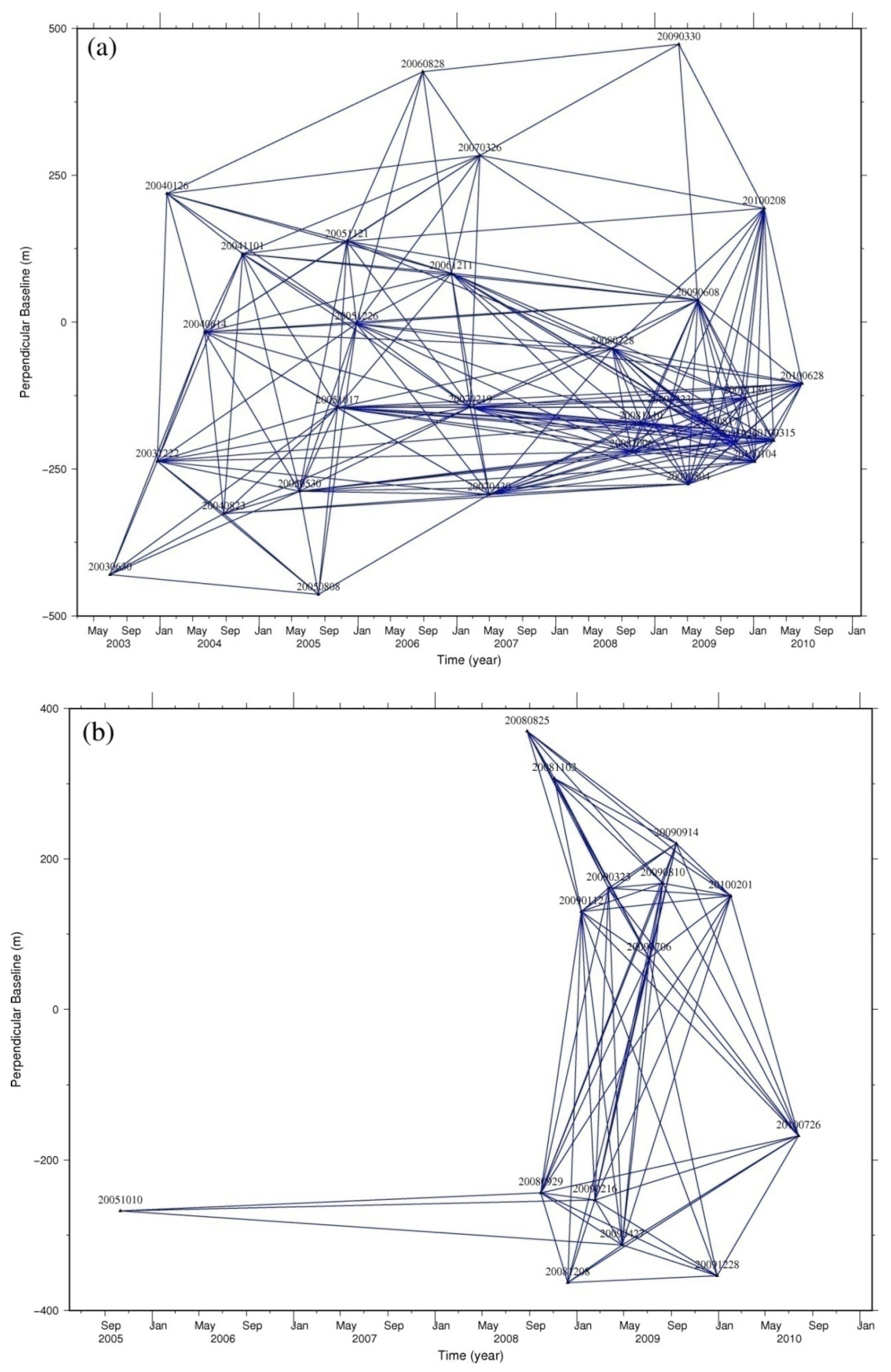
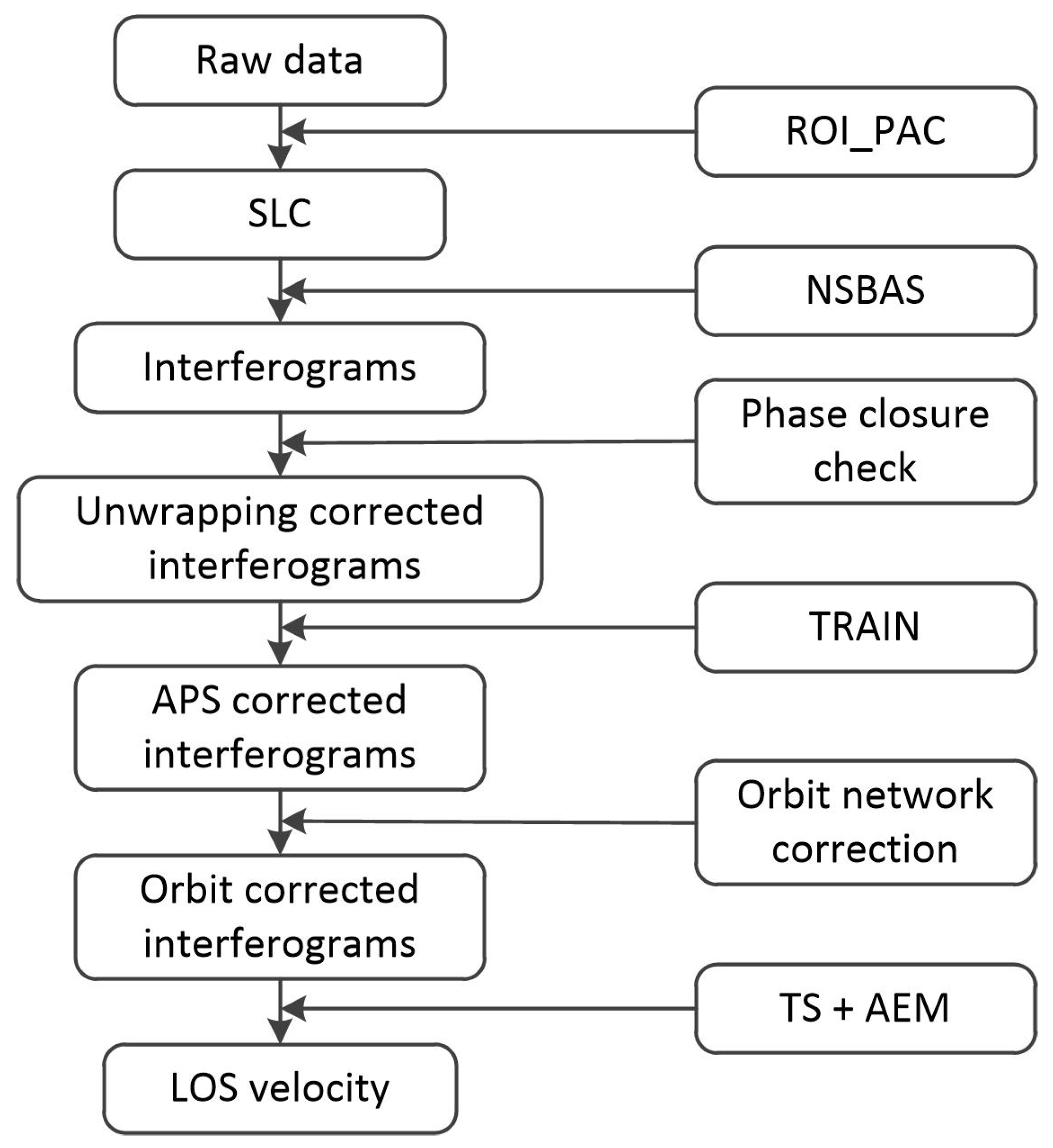
2.1. InSAR Data and Processing

Synthetic aperture radar images from the advanced SAR (ASAR) instrument on board the ENVISAT satellite were used in this study to investigate interseismic deformation across the ATF at 85°E. The data set was acquired between June 2003 and June 2010, and includes 33 descending images and 15 ascending images. The raw data were processed with repeat orbit interferometry package (ROI_PAC) Version 3.1 beta [30]. Precise DORIS orbital data for ENVISAT satellite provided by ESA has been used for interferometric processing. All of the interferograms were produced using the NSBAS package [31,32]. Image pairs were selected by spatial and temporal baselines: (i) B_t < 1 year and B_s < 500 m; (ii) B_t < 3 year and B_s < 300 m; and (iii) B_t < 5 year and B_s < 100 m (Figure 2). In ascending track 298, the 10 October 2005data extends the time baseline from 2 to 5 years, which is significant for the time series deformation analysis. Unlike ROI_PAC, the NSBAS takes into account the DEM when co-registering images [33], which improved the interferometric processing and increased the coherence of interferograms.

During SAR data processing, we multilooked the SAR images 4 and 20 times in the azimuth and range directions, respectively, during processing to improve the signal-to-noise ratio. The phase component of the topography was removed using the three-arc second shuttle radar topography mission (SRTM) DEM [34] with the ESA DORIS precision orbits. A power spectrum filter [35] was applied to further reduce the phase noise to improve the interferogram coherence. Most interferograms were unwrapped using the branch-cut method [36], but some of them needed manual unwrapping (bridge) across the fault due to the loss of coherence. The unwrapping errors were detected and removed by a phase-closure technique [37,38]. After phase closure check, we correct the atmospheric errors and orbital ramps (Figure 3) respectively. The whole process flow is summarized in Figure 4. The coherence of north areas of the ATF was commonly higher than that of the southern part because of snow cover on the southern mountains (Figure 5). Areas near the ATF have poor coherence even compared with the southern part as a result of the topography.

2.2. Atmospheric Correction

The greatest factor limiting InSAR measurement accuracy is atmospheric delay, particularly from tropospheric water vapor [39].This is exacerbated for the ATF due to its relief of ~4 km [16]. Crustal deformation signals measured over short time scales are dominated by orbital and atmospheric errors. The atmospheric phase delay, mainly derived from the temporal variation of stratified troposphere, may reach tens of centimeters [40,41].

There are two groups of correction methods to estimate atmospheric phase delay, the empirical and the predictive methods. Assuming that the relationship between the atmospheric delays and elevation is approximately linear, a first order function [16,41,42] could be used to estimate the conversion coefficient. Unfortunately, empirical methods cannot be easily used when the expected deformation signal correlates with topography, which is the case for such major topographic steps like ATF [16]. Predictive methods are based on inputs from external data sets to compute synthetic delay maps and directly correct for tropospheric delays in interferograms. The external data sets include local meteorological data [43], GPS zenith delay measurements [44,45,46,47], satellite multi-spectral imagery [48,49], and outputs from local meteorological models constrained by local data collection [50,51,52]. These external data have proven successful and accurate for atmospheric correction; however, rarely available local data limit the popularity of this method.

Here, we use the method from Bekaert et al. [33,53,54] to estimate the atmospheric phase delay maps using the ERA-I global atmospheric model reanalysis product [55] obtained from the European Center for Medium-Range Weather Forecasts. The ERA-I provides estimates of temperature, water vapor partial pressure, and geopotential height along 37 pressure levels, on a global 0.7° × 0.7° grid at regular 6-hour intervals from 1989 to present. Both hydrostatic and wet contributions to the phase delay are taken into account in this approach (Figure 3). This method accounts for spatial variability of the tropospheric properties and successfully captures tropospheric signals over large regions. In Figure 3, for example, we removed the elevation-correlated atmospheric path delay from original observations to correct for atmospheric errors; in Figure 3b, the clear difference across the fault in Figure 3a is removed denoting the reduction of the elevation-correlated atmospheric delay. We have calculated the standard deviation(σ) reduction of the APS correction and find that σ is reduced in 38% by ECMWF-based correction. The results confirm that the ERA-I model can overcome limitations of empirical models [56].

2.3. Orbital Correction

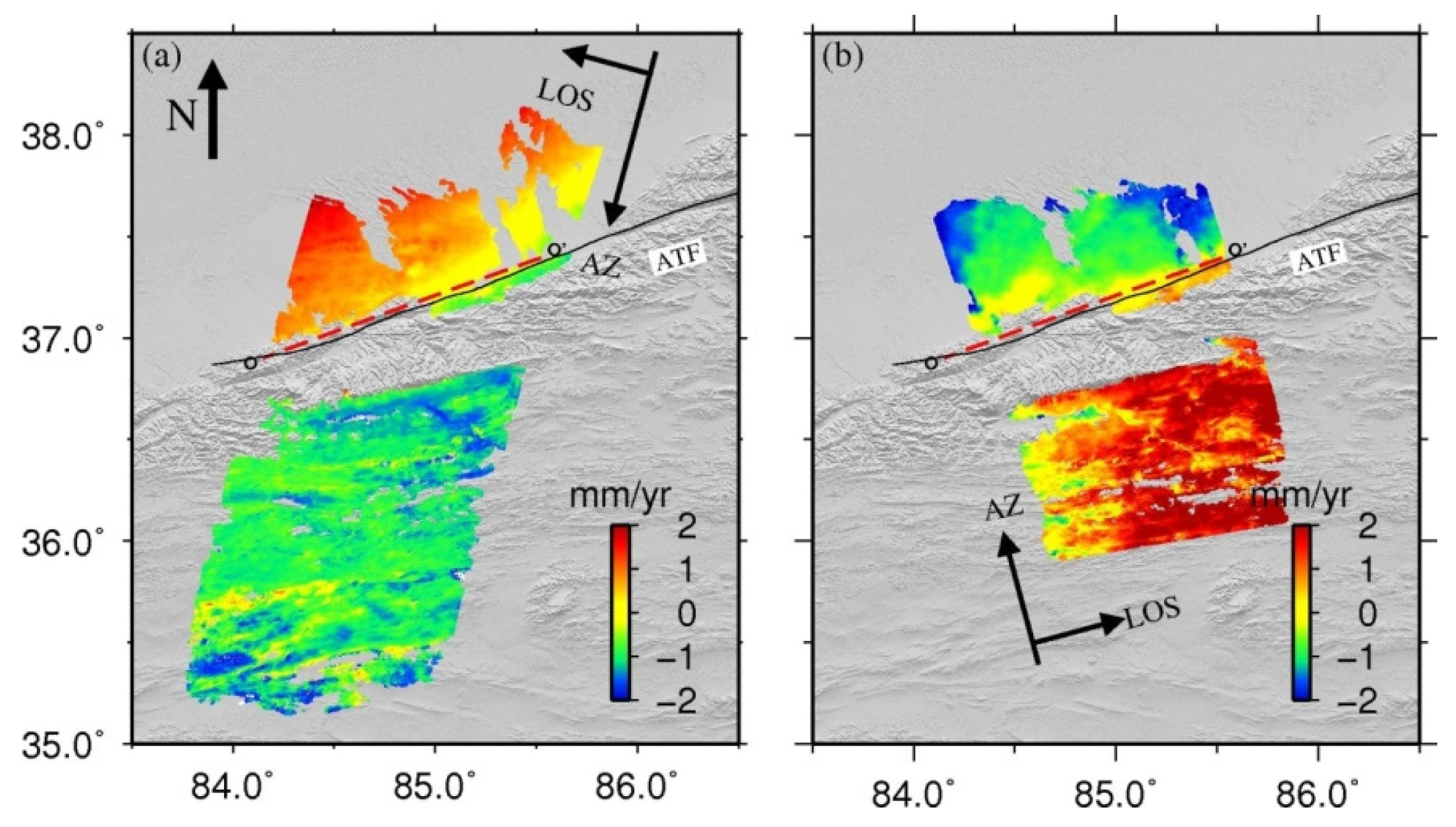
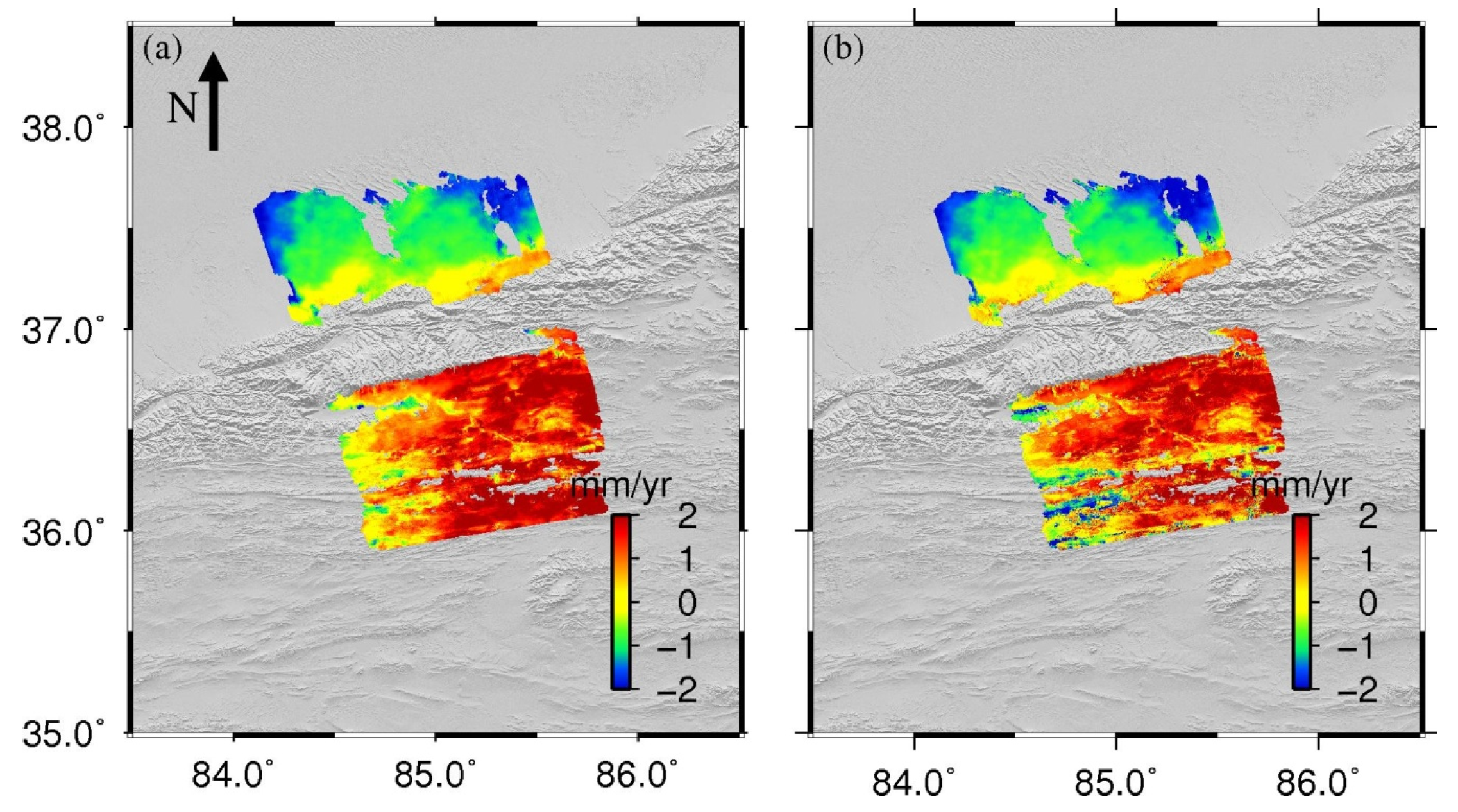
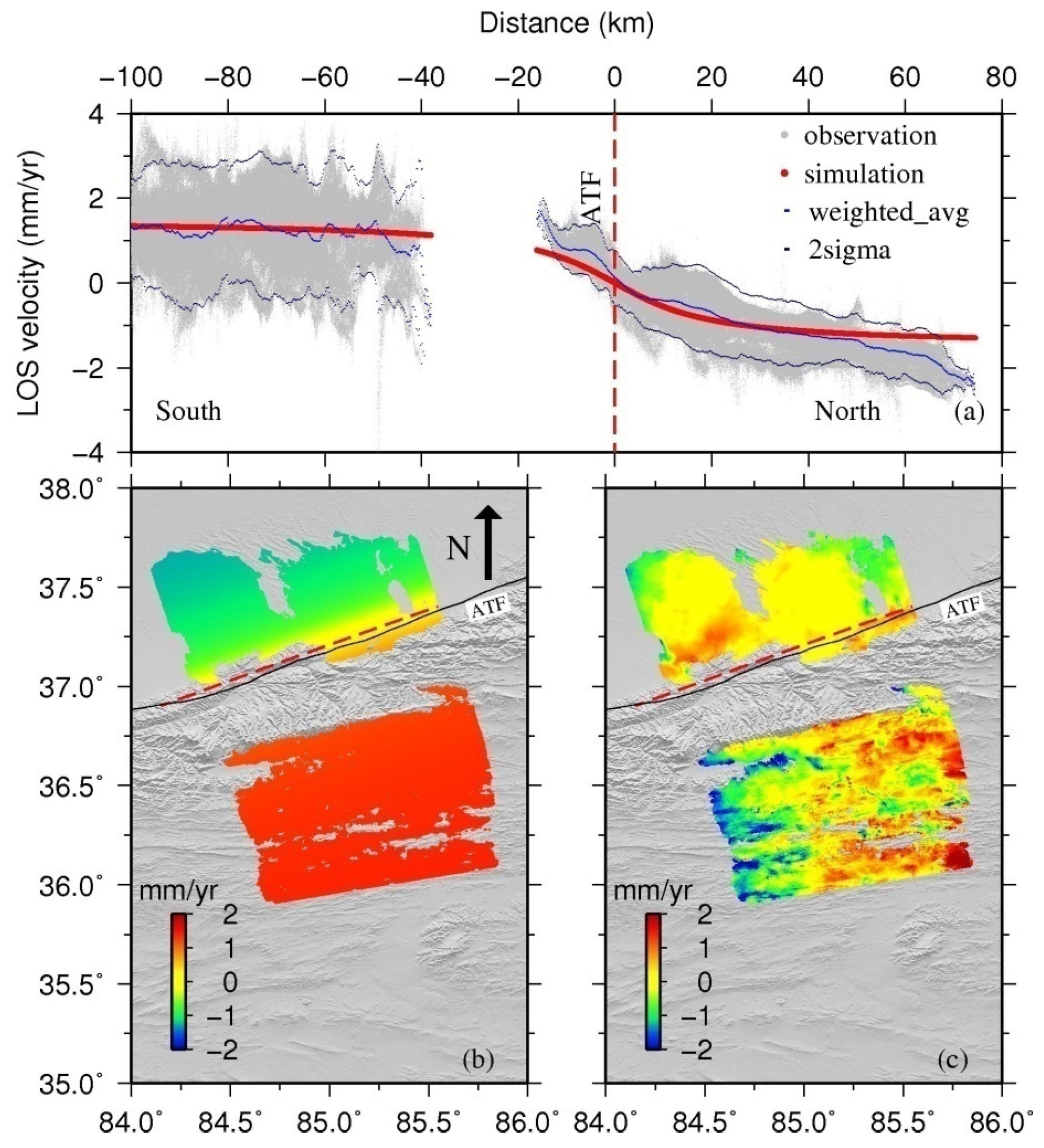
Because of our imperfect knowledge of the state vector of the ENVISAT satellite, even after the effects of baseline separation have been removed, an orbital error remains in the interferogram [57]. A clear linear ramp is shown in atmospheric corrected interferogram (Figure 3b). It is caused by long wavelength orbital errors and the orbital correction is needed before further processing. A linear approximation is usually sufficiently accurate for short strips (100–200 km along track) and a quadratic approximation is required for longer strips. This approach is sufficient because the deformation signal represents a small portion of interferometric phase, such as volcanology and earthquakes [58]. Hence, it is possible to define a “far-field” area of the interferogram and to re-estimate the baseline parameters [37]. However, there is no true “far-field” in such a large area for studies of interseismic deformation, so the baseline for individual interferograms to deal with the orbital contributions cannot be precisely re-estimated.

For this reason, Biggs et al. [37] presented a global network orbital correction method to deal with the issue of orbital contributions at a later stage of re-estimating the baseline. Here, we use this method to remove orbital errors remaining in the interferograms (Figure 3c). It can be seen from Figure 3c that a phase ramp is removed from the atmospheric corrected interferogram (Figure 3b) after the network orbital correction. The σ reduction of this step is 13% of the interferogram. This correction technique also accounts for other long wavelength signals, such as ionospheric and long wavelength tropospheric contributions as well as errors in orbit [37].

2.4. Rate Map

A LOS rate map is calculated from the interferograms corrected for both atmospheric and orbital errors using the InSAR TS + AEM package developed at the University of Glasgow based on the SBAS algorithm [59,60,61] as the flow chart in Figure 4. The RMS between LOS deformation derived from the InSAR TS + AEM package and GPS measurements is smaller than 0.5 mm/year, which was validated independently by Li et al. (Abstract G13B-07 presented at Fall Meeting. 2010, AGU, San Francisco, CA, USA) and Hammond et al. [62].

We obtained the deformation rate map for the ATF from corrected interferograms using the InSAR TS + AEM approach (Figure5). It indicates that the deformation rate of ATF ranges from –2 mm/year to 2 mm/year in the LOS direction. One clear point is that the LOS velocity changes across the ATF in both tracks. The opposite gradient trends on ascending and descending tracks were consistent with left-lateral motion of the ATF system. There is no clear correlation between the topography and the mean-velocity map, indicating that the topography-related atmospheric errors have been successfully removed and that no significant residual atmospheric effect related to the topography is affecting the results.

To test the effect of the isolated 10 October 2005 acquisition to the final velocity results, we performed the inversion without the 10 October 2005 data. The result is shown in Figure 6: the left one (Figure 6a) is the velocity of data set including 10 October 2005 data, whereas the right one (Figure 6b) is velocity result from data set without 10 October 2005 data. From the velocity map we can know that the 10 October 2005 data actually affects the result in some degree (the range of LOS velocity changes from –2.00~1.72 mm/year of data set including 10 October 2005 data to –2.20~1.92 mm/year without 10 October 2005 data), however the first-order deformation characteristics is consistent with the results obtained from all the dataset.

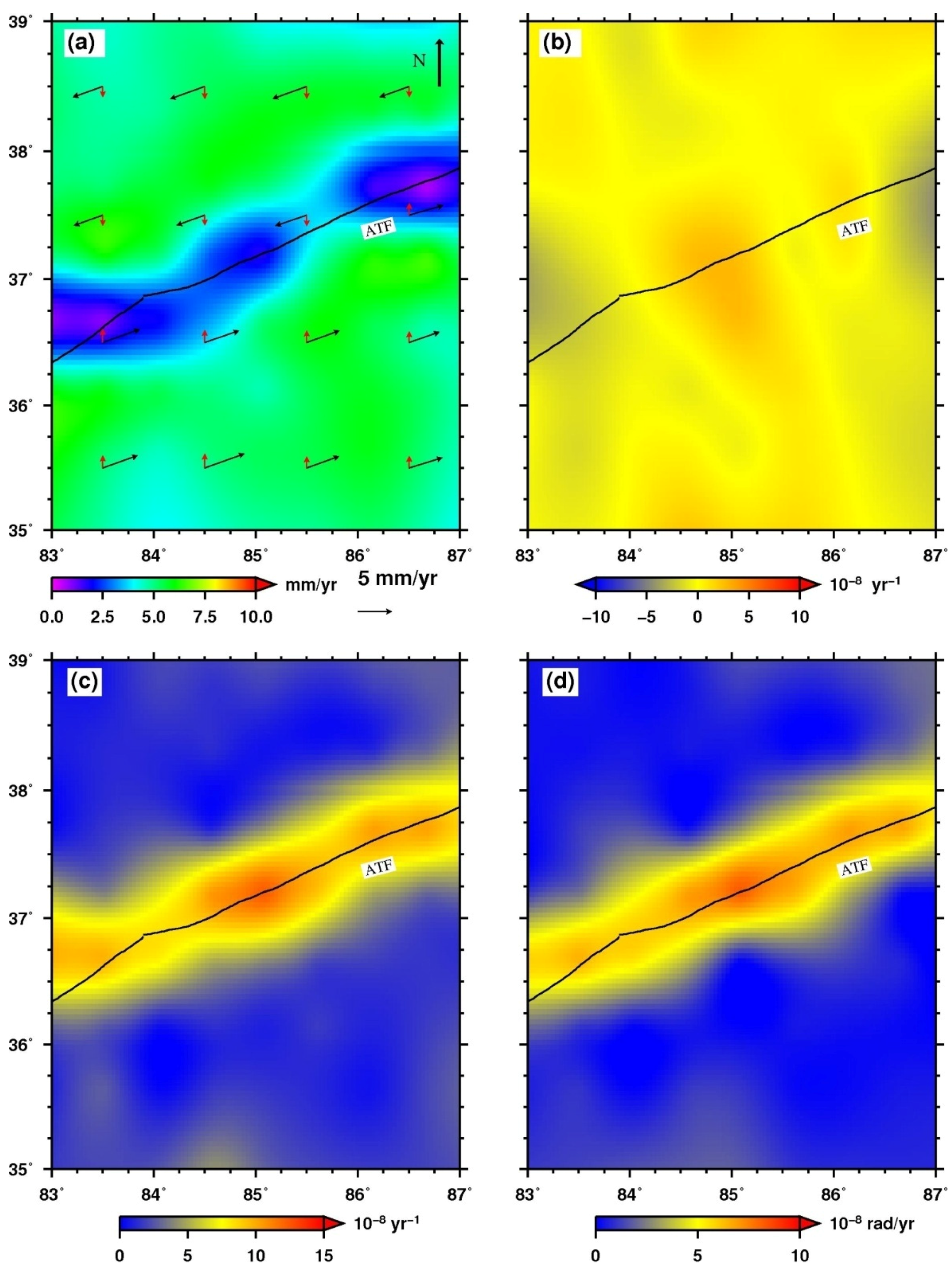
2.5. Strain Rate Map

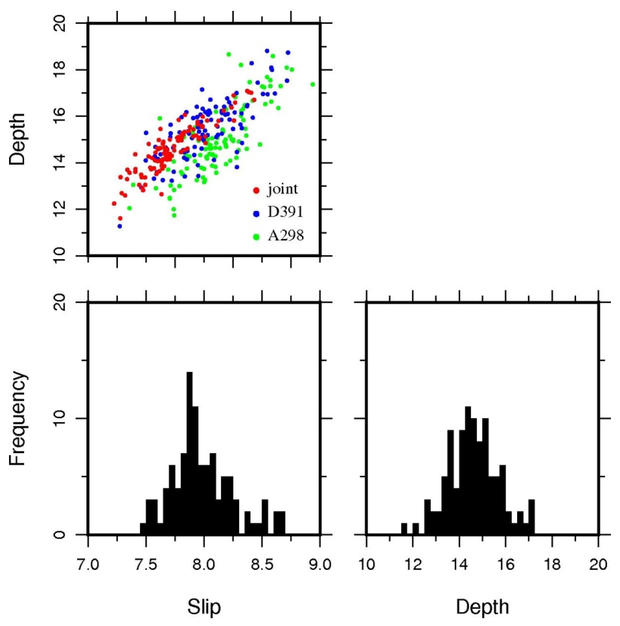
Strain fields of a region describe the geometric changes caused by deformation and, therefore, its characteristic pattern and amplitude are very important to understanding the present-day tectonic processes and underlying driving forces in this area. The strain rate tensor can be used to study crustal deformation and characterize geodynamic processes, such as strain accumulation, independent of a reference frame. Therefore, it is common to derive the distribution of strain rate fields to capture the tectonic mechanism of a region.

To better constrain the deformation characteristics of the ATF, we calculated the strain rate field in the spherical coordinates from velocity fields using the wavelet-based multi-scale estimation method proposed by Tape et al. [26]. This method can localize a given deformation field in space and scale as well as detect outliers in the observation set. Based on the relative less normal deformation from a GPS study [11], we resolved the along-fault velocity using ascending and descending track LOS velocities and used it as the total horizontal velocity. Then we extrapolated the velocity field of this area using the Kriging interpolation method (Figure 7a). Finally, we calculated the three invariant quantities, related dilatation rate, strain rate and rotation rate, which do not depend on the coordinate system.

The strain rate field (Figure 7c) exhibits the expected interseismic pattern for a locked fault with a maximum along the fault and symmetric on either side. Strain accumulation is strongly localized on the ATF. The northern Tarim Basin and southern high plateau regions are straining at very low rates in comparison to the major strike-slip faults. The maximum strain rate along the fault is approximately 12.4 × 10⁻⁸/year. The dilatation rate was nearly zero. The rotation rate has a maximum of approximately 10 × 10⁻⁸/year, indicating that rotation can partly account for the deformation in the vicinity of the fault. In comparison to previous studies, our results are consistent in one-order features, although we only calculate the strain rate field across the ATF rather than the whole Tibetan Plateau. The strain rate fields in Figure 7c reproduce the same first-order features as the velocity field, and show that strain is strongly focused on the main left-lateral strike-slip fault. In this study, we have shown that it is possible to create 2-D strain maps using InSAR data from two observations, even in the absence of GPS observations.

3. Modeling

As seen from the strain field in Figure 7c, the strain strongly focused on the main left-lateral strike-slip fault, so we can assume that the main contributions to the deformation are from the ATF. To aid in the interpretation of the first-order characteristics of the LOS velocity map, a simple elastic model with single fault geometry was used to invert the slip-rate and locking depth of the ATF. Although one more complex model may be more appropriate for this fault, the lack of data near the fault makes it hard to constrain the deformation using a complex model. Consequently, we assumed a strike-slip fault with 90° dip angle. We assumed that LOS deformation is a combination of fault parallel deformation and vertical deformation, ignoring normal fault deformation, which is justified by GPS measurements [11]. We modeled the fault as a buried infinite screw dislocation in a homogeneous, isotropic elastic half-space, where aseismic slip occurs at a rate (s) below a locking depth (d) during the interseismic period.

Under this assumption, we converted displacement of two profiles in LOS direction into horizontal displacements parallel to the fault and vertical displacements. We accounted for both horizontal and vertical displacement with two data tracks in our inversion rather than accounting for only horizontal displacement [16] with only one track, in our inversion process the contribution from vertical components is subtracted from the InSAR observations. The relationship between LOS displacements and horizontal and vertical displacement is given by:

$$d_{los}=u_{n}sin\phi sin\theta -u_{e}cos\phi sin\theta +u_{u}cos\theta$$

(1)

where $\phi$ is the azimuth angle for the satellite orbit, $\theta$ is the incidence angle, and u_(n,e,u) are the north, east, and up components of displacement, respectively. We decomposed the horizontal component of the fault to parallel and normal components and ignored the normal component. As it is one-third smaller with respect to the parallel component and nearly vertical to the LOS direction, its projection to the LOS is negligible. Thus, Equation (1) can be rewritten as:

$$d_{los}=u_{h}cos\alpha sin\theta +u_{u}cos\theta$$

(2)

where $\alpha$ is the angle between the fault line and horizontal projection of LOS. We thus have two unknowns (u_h, u_u) and two equations, so it is possible to solve the equations.

The slip rate (s) and locking depth (d) of the fault were determined based on the Savage and Burford [63] analytical solution, which explains the surface velocity (y) parallel to the fault at a given distance (x) from the fault as:

$$y=\frac{s}{\pi }ta{n}^{-1}\frac{x}{d}$$

(3)

We performed an initial parameter search over the 0.5–10.0 mm/year for slip rate and 5–35 km locking depth with the simulated annealing algorithm [64,65]. Our best-fit model for joint inversion, corresponding to the minimum of RMS misfit, yields a slip rate of 8.0 mm/year and a locking depth of 14.5 km. The simulation and residuals between observations and simulating results of D391 and A298 are presented in Figure 8 and Figure 9 respectively. The residuals of A298 are not as smooth as D391. This probably results from fewer image dates in the inversion, which again confirms that additional observations can reduce errors.

Regarding error associated with these fault parameters, the main source remaining in the mean velocity map is related to residual turbulent atmospheric perturbations and orbital error in the interferograms. Therefore, we attempted to estimate the impact of such perturbations in the fault parameters by generating 100 perturbed mean velocity maps and then using the same inversion scheme as for the non-perturbed dataset. The parameter uncertainties were determined using the standard deviation of the slip and locking depth estimate from the 100 runs, which resulted in a slip rate of 8.0 ± 0.7 mm/year and 14.5 ± 3 km for locking depth (Figure 10).

We also performed the parameter search for each track data and assumed no vertical displacements. The best-fit parameters for D391 are 8.2 mm/year of slip and a locking depth of 16 km (blue dots in Figure 10), whereas the best-fit parameters for A298 are a slip rate of 8.3 mm/year and 14.8 km of locking depth (green dots in Figure 10). The results from the two tracks are in good agreement with each other. Figure 8 and Figure 9 show profiles of the LOS velocity perpendicular to the strike direction of the ATF for the descending and ascending tracks, respectively, which are consistent overall with a classic arctangent shape predicted by screw dislocation models across strike-slip faults [63]. The residual maps show that the LOS velocity of the descending track (D391) fits well with the model, whereas the ascending track (A298) has some significant misfits in the southern part. This may be caused by unwrapping errors or less coherence resulting from a smaller number of SAR images.

The joint inversion results of both tracks are slightly slower because we ignored the vertical fault motion contribution in the single track inversion, as it is small relative to horizontal motion along the fault. We note that the joint inversion results are more concentrated near the best-fit parameters than the single track inversion, which demonstrates the importance of including the vertical displacements to better constrain the ATF deformation. The uncertainty for both slip rate and locking depth was reduced using SAR data from two directions as opposed to one single direction.

4. Discussion

After planar orbital and linear atmospheric corrections, we computed the strain rate fields using a multi-scale wavelet method. The strain fields show that deformation across the ATF is concentrated on the fault. England and Molnar [2] calculated crustal velocity fields and strain rates within Asia from estimates of Quaternary slip rates on faults and baseline length rates between GPS sites. They suggested that the strain rate fields determined by geodetic measurements taken on a decadal timescale are consistent with geological observations on a 10⁴ years timescale. Allmendinger et al. [66] derived 2-D strain and rotation rate fields from a GPS velocity field using both the nearest neighbor and distance weighted approach. Their results showed that the principal infinitesimal strain rate axes in Tibet are consistent with large, long term geological structures similar to England and Molnar [2]. Gan et al. [67] deduced the strain rate fields using ~726 GPS velocities around the plateau after removing the rotational component of the entire plateau. Although the method and data set are different from England and Molnar [2], their results were generally consistent in all of the relevant areas within the plateau. Our strain fields are consistent with the first-order characteristics across the major faults from previous studies [2]. This study confirms the possibility of creating 2-D strain rate maps from InSAR data and also shows that InSAR observations can constrain velocity and strain maps with respect to GPS data.

We inverted the slip rate and fault depth using a screw dislocation model. Our preferred model implies a left-lateral displacement rate across the ATF of 8.0 ± 0.7 mm/year and 14.5 ± 3 km locking depth. The locking depth was not as well constrained as the other geodetic inversion results [14]. We note that the slip rate is in good agreement with GPS measurements of 9 ± 4 mm/year [17] almost 1° east of our study area. It is also consistent with InSAR results of 11 ± 5 mm/year estimated from ERS data [16]. Similar to other geodetic measurements [15,16,17,68], we also identified the asymmetric deformation pattern between the two sides of the fault. The possible mechanisms to explain this interseismic velocity asymmetry maybe a variation of the elastic crustal thickness from rheological contrast on two sides of the ATF [68] or variation in fault dip angle.

Our results differ significantly from slip rates determined by geological methods (27 ± 7 mm/year; [18]) based on detailed measurements of different geomorphic terrace riser offsets using radiocarbon and cosmic ray dating. The discrepancy between these two methods could be due to the different time scales if both methods have no errors or slip rates vary with time like faults in Southern California [69]. Cowie et al. reported earlier that fault slip rates can vary in time or along strike the fault, both due to clustering or quiescence periods of the fault activity or due to long term effects [70,71]. Roberts et al. showed the first example of such fault slip rate variability from active faults [72]. Burchfiel et al. [73] suggested that whether the geodetically observed slip rates recorded over the last 5–10 years agree or are representative to the longer-term geologically derived slip rates is debetable. Indeed there are several examples where such a discrepancy occurs between geological and geodetic rates in several settings worldwide (e.g., Papanikolaou et al. [74]; Kenner and Simons, [75]) However, some geological authors suggest a low slip rate of the ATF that is consistent with our results. Yin et al. [76] derived an average rate of 9 ± 2 mm/year since 49 Ma. This significant difference was reconciled by geologic [77] and recent geodetic [17] data, which both agree on a slip rate of 9.0 ± 4.0 mm/year. As Cog will et al. [77,78] argued that the apparent discrepancy in slip rate along this fault might result more from systematic biases in geomorphic reconstructions rather than from true secular variation in slip rate.

Our consistent low slip rates along the fault are in consistent with the historical seismicity in this region. Only two great historical earthquakes have occurred along the ATF, both in 1924 west of 85°E [79,80]. In fact, contemporary instrumental recordings also show a low level of seismicity along the ATF. Paleoseismo logical studies suggest recurrence intervals of major earthquakes in the range of 700 ± 400 and 1100 ± 300 years for offsets of 4 and 7 m, respectively, consistent with a slip rate of ~10 mm/year [79,81,82].

Elliott et al. [16] measured the interseismic slip rate of the ATF using a stacking method with one single descending track of ERS data (1993–2000); their slip rate estimate was 11 ± 5 mm/year with significant uncertainty. Here, we used the InSAR TS + AEM method with 7 years (2003–2010) of ENVISAT ASAR data and both ascending and descending tracks; our slip rate estimate was 8.0 ± 0.7 mm/year. Our results are in agreement with results of Elliott et al. from ERS data [16] and GPS measurements (9 ± 4 mm/year; [17]). We used the same track ENVISAT ASAR data as [16] with an additional two years of descending track data and five years of ascending track data. The difference in slip rates between our study and Elliott et al. [16] is probably a result of time-varying slip rate or stacking method assumptions that the atmospheric effect was normally distributed. However, because the topographic variation across the ATF is large, maybe it is not appropriate to assume normal distribution atmospheric errors. We had to remove any topography-correlated atmospheric errors. This study again demonstrates the importance of atmospheric and orbital corrections in InSAR time series processing. We determined our slip rate from 216 interferograms, while they used only 66 interferograms, which possibly cannot constrain the InSAR slip rate as well. Additionally, because we used ascending and descending track data, we were able to calculate the velocity parallel to the ATF as well as vertical velocity from two observing geometries and thus remove the projection of vertical deformation velocity from the LOS velocity. Elliott et al. [16] simply ignored the vertical velocity whose contributions are subtracted from the InSAR observations in our study, so their result was a little higher than ours. It is likely our calculated velocity is closer to the real velocity. We were also able to reduce the range of uncertainty for both slip rate and locking depth using two look directions of data because we used both descending and ascending track data, in comparison to the results of [16] that are based on descending track data only. This improvement demonstrates the importance of using SAR data from two look directions for interseismic studies.

It is worth noting that we simplify the model by disregarding deformation produced by the other possible surrounding secondary faults in the study area. The real tectonic setting is definitely more complex than the simple model we have used in this study. The reasons we used this simple model are that reliable SAR data near the fault were not available, which may be insufficient for a distributed slip inversion in this case; and the fault-normal and vertical deformations across the ATF are relative less with respect the strike slip [1,2,14,15]. Our results may include contributions of surrounding secondary faults or other mechanisms like the shrinkage or expansion of clay minerals, or even excessive water pumping or significant seasonal variations of the water table. In addition, our SAR data covered only seven years, the low temporal resolution results prevent us from extracting the varying history of fault slip rate and locking depth. Our SAR data covered only a segment of the whole ATF, we assume that our results from SAR data can represent the first-order deformation characteristics of the ATF. The detailed deformation needs further geodetic or geological study.

In Figure 7a, we have shown the vertical component of the interpolated LOS velocity obtained from two tracks of SAR data. If we assumed that the Tarim basin is static, then the south part across the ATF is uplifting with respect to the Tarim basin with nearly 3 mm/year velocity in agreements with Bendickand coworkers’ [14] and England and Molnar’s [1] results. England and Molnar [1] estimated a shortening rate of 6 ± 4 mm/year across the central section of the ATF. Bendick et al. [14] reported a contraction rate of 3 ± 1 mm/year across the same section. Chen et al. [83] estimated 5 ± 2 mm/year across the east section at ~95°E. Shen et al. [15] estimate 0 ± 2 mm/year convergence across the central Altyn Tagh system, which indicates strongly that north-south shortening across the ATF is negligible. Also, geologic mapping along the NATF by Cog will et al. [84] suggested that it is mostly a left slip fault with only minor compression.

Previous geodetic results based on GPS [14,17,79] and InSAR [16,68] data suggested a slip rate of~10 mm/year at different points across the ATF. Our interseismic strain accumulation profiles across the ATF are in good agreement with these previous GPS measurements and InSAR results. The slip rates and locking depth for the ATF estimated from both GPS and InSAR studies and from geological studies [77,78] are also consistent with our results. This consistency indicates that the ATF played only a secondary role in the northeastward extrusion of material in the Tibetan Plateau [79], with most of the extrusion occurring in the interior of the plateau. Therefore, our results are close to the continuum models of Asian deformation requiring low fault slip rates [2,85].

5. Conclusions

Using a multi-scale wavelet method, we calculated the strain rate fields of the ATF region and determined that the strain was mainly localized along the fault, which is generally consistent with previous studies. We also show that high-resolution 2-D strain rate fields can be determined from InSAR data alone, especially in regions with spatially sparse GPS data. Based on the orbital ramp and atmospheric effect correction, we inverted the slip rate and locking depth using a screw dislocation model with ascending and descending track ENVISAT data. We performed the inversions for single track data and jointly. Our joint inversion result indicates that the ATF has a slip rate of 8.0 ± 0.7 mm/year and locking depth of 14.5 ± 3 km. The joint inversion slip rate is a little slower than the single track inversion because of vertical deformation in the inversion. Our results are more accurate than those of Elliott et al. [16] owing to a greater number of observations in our study and the fact that we accounted for the vertical deformation in the inversion process. This study shows the importance of using both descending and ascending data in interseismic InSAR studies. As a result of the more frequent data acquisition from satellite missions, such as Sentinel-1A, ALOS-2 and the upcoming Sentinel-1B, similar studies will become increasingly common. The relative low slip rate indicates that the ATF does not transfer a significant part of the convergence between India and Asia into the northeastward extrusion of the Tibetan Plateau [76], and the deformation pattern is close to the continuum deformation models [2].

References

1. England, P.; Molnar, P. Active deformation of Asia: From kinematics to dynamics. Science 1997, 278, 647–650. [Google Scholar] [CrossRef]
2. England, P.; Molnar, P. Late Quaternary to decadal velocity fields in Asia. J. Geophys. Res. 2005, 110, B12401. [Google Scholar] [CrossRef]
3. Meade, J. Present-day kinematics at the India-Asia collision zone. Geology 2007, 35, 81–84. [Google Scholar] [CrossRef]
4. Thatcher, W. Microplate model for the present-day deformation of Tibet. J. Geophys. Res. 2007, 112, B01401. [Google Scholar] [CrossRef]
5. Zhang, L.; Ye, G.; Jin, S.; Wei, W.; Unsworth, M.; Jones, A.; Jing, J.; Dong, H.; Xie, C.; Le Pape, F.; et al. Lithospheric electrical structure across the Eastern Segment of the Altyn Tagh Fault on the Northern Margin of the Tibetan Plateau. Acta Geol. Sin. 2015, 89, 90–104. [Google Scholar]
6. Molnar, P.; Tapponnier, P. Cenozoic tectonics of Asia: Effects of a continental collision. Science 1975, 189, 419–426. [Google Scholar] [CrossRef] [PubMed]
7. Avouac, J.-P.; Tapponnier, P. Kinematic model of active deformation in central Asia. Geophys. Res. Lett. 1993, 20, 895–898. [Google Scholar] [CrossRef]
8. Zhang, P.Z.; Shen, Z.K.; Wang, M.; Gan, W.; Bürgmann, R.; Molnar, P.; Wang, Q.; Niu, Z.; Sun, J.; Wu, J. Continuous deformation of the Tibetan Plateau from Global Positioning System data. Geology 2004, 32, 809–812. [Google Scholar] [CrossRef]
9. Wittlinger, G.; Tapponnier, P.; Poupinet, G.; Jiang, M.; Shi, D.; Herquel, G.; Masson, F. Tomographic evidence for localized lithospheric shear along the AltynTaghFault. Science 1998, 282, 74–76. [Google Scholar] [CrossRef] [PubMed]
10. Burchfiel, B.C.; Deng, Q.; Molnar, P.; Royden, L.; Wang, Y.; Zhang, P.; Zhang, W. Intracrustal detachment within zones of continental deformation. Geology 1989, 17, 748–752. [Google Scholar] [CrossRef]
11. Ge, W.-P.; Molnar, P.; Shen, Z.-K.; Li, Q. Present-day crustal thinning in the southern and northern Tibetan Plateau revealed by GPS measurements. Geophys. Res. Lett. 2015, 42, 5227–5235. [Google Scholar] [CrossRef]
12. Wallace, K.; Yin, G.; Bilham, R. Inescapable slow slip on the Altyn Tagh Fault. Geophys. Res. Lett. 2004, 31, L09613. [Google Scholar] [CrossRef]
13. Houseman, G.; England, P. Crustal thickening vs. lateral expulsion in the Indian-Asian continental collision. J. Geophys. Res. 1993, 98, 12233–12249. [Google Scholar] [CrossRef]
14. Bendick, R.; Bilham, P.; Freymueller, J.T.; Larson, K.M.; Yin, G. Geodetic evidence for a low slip rate in the Altyn Tagh fault system. Nature 2000, 386, 61–64. [Google Scholar]
15. Shen, Z.-K.; Wang, M.; Li, Y.; Jackson, D.D.; Yin, A.; Dong, D.; Fang, P. Crustal deformation along the Altyn Tagh fault system, western China, from GPS. J. Geophys. Res. 2001, 106, 30607–30622. [Google Scholar] [CrossRef]
16. Elliott, J.R.; Biggs, J.; Parsons, B.; Wright, T.J. InSAR slip rate determination on the Altyn Tagh Fault, northern Tibet, in the presence of topographically correlated atmospheric delays. Geophys. Res. Lett. 2008, 35, L12309. [Google Scholar] [CrossRef]
17. He, J.; Vernant, P.; Chéry, J.; Wang, W.; Lu, S.; Ku, W.; Xia, W.; Bilham, R. Nailing down the slip rate of the AltynTaghFault. Geophys. Res. Lett. 2013, 40, 5382–5386. [Google Scholar] [CrossRef]
18. Mériaux, A.-S.; Ryerson, F.J.; Tapponnier, P.; Van der Woerd, J.; Finkel, R.C.; Xu, X.; Xu, Z.; Caffee, M.W. Rapid slip along the central Altyn Tagh Fault: Morphochronologic evidence from Cherchen He and Sulamu Tagh. J. Geophys. Res. 2004, 109, B06401. [Google Scholar] [CrossRef]
19. Rosen, P.A.; Hensley, S.; Zebker, H.A.; Webb, F.H.; Fielding, E.J. Surface deformation and coherence measurements of Kilauea Volcano, Hawaii, from SIR-C radar interferometry. J. Geophys. Res. Planets 1996, 101, 23109–23125. [Google Scholar] [CrossRef]
20. Massonnet, D.; Rossi, M.; Carmona, C.; Adragna, F.; Peltzer, G.; Feigl, K.; Rabaute, T. The displacement field of the Landers earthquake mapped by radar interferometry. Nature 1993, 364, 138–142. [Google Scholar] [CrossRef]
21. Wright, T.; Parsons, B.; Fielding, E.J. Measurement of interseismic strain accumulation across the North Anatolian Fault by satellite radar interferometry. Geophys. Res. Lett. 2001, 28, 2117–2120. [Google Scholar] [CrossRef]
22. Walters, R.J.; Holley, R.J.; Parsons, B.; Wright, T.J. Interseismic strain accumulation across the North Anatolian Fault from Envisat InSAR measurements. Geophys. Res. Lett. 2011, 38, L05303. [Google Scholar] [CrossRef]
23. Xu, C.J.; Wang, H.; Jiang, G.Y. Study on crustal deformation of Wenchuan Ms8.0 earthquake using wide-swath scan SAR and MODIS. Geod. Geodyn. 2011, 2, 1–6. [Google Scholar]
24. Liu, Y.; Xu, C.J.; Wen, Y.M. InSAR measurement of surface deformation between two Da-Qaidam Mw6.3 earthquakes and joint analysis with coseismic rupture. Geod. Geodyn. 2016, 36, 110–114. [Google Scholar]
25. Papanikolaou, I.D.; Balen, R.V.; Silva, P.G.; Reicherter, K. Geomorphology of active faulting and seismic hazard assessment: New tools and future challenges. Geomorphology 2015, 237, 1–13. [Google Scholar] [CrossRef]
26. Tape, C.; Musé, P.; Simons, M.; Dong, D.; Webb, F. Multiscale estimation of GPS velocity fields. Geophys. J. Int. 2009, 179, 945–971. [Google Scholar] [CrossRef]
27. Walters, R.J.; Parsons, B.; Wright, T.J. Constraining crustal velocity fields with InSAR for Eastern Turkey: Limits to the block-like behavior of Eastern Anatolia. J. Geophys. Res. 2014, 119, 5215–5234. [Google Scholar] [CrossRef]
28. Garthwaite, M.C.; Wang, H.; Wright, T.J. Broadscale interseismic deformation and fault slip rates in the central Tibetan Plateau observed using InSAR. J. Geophys. Res. Solid Earth 2013, 118, 5071–5083. [Google Scholar] [CrossRef]
29. Ryder, I.; Parsons, B.; Wright, T.J.; Funning, G. Post-seismicmotion following the 1997 Manyi, Tibet earthquake, InSAR observations and modelling. Geophys. J. Int. 2007, 169, 1009–1027. [Google Scholar] [CrossRef]
30. Rosen, P.A.; Henley, S.; Peltzer, G.; Simons, M. Update repeat orbit interferometry package released. Eos Trans. AGU 2004, 85, 47. [Google Scholar] [CrossRef]
31. Doin, M.P.; Guillaso, S.; Jolivet, R.; Lasserre, C.; Lodge, F.; Ducret, G.; Grandin, R. Presentation of the small baseline NSBAS processing chain on a case example: The Etna deformation monitoring from 2003 to 2010 using Envisat data. In Proceedings of the European Space Agency Symposium “Fringe”, ESA SP-697. Frascati, Italy, 19–23 September 2011.
32. NSBAS. Available online: http://efidir.poleterresolide.fr/index.php/effidir-tools/nsbas (accessed on 8 March 2016).
33. Doin, M.P.; Lasserre, C.; Peltzer, G.; Cavalie, O.; Doubre, C. Corrections of stratified tropospheric delays in SAR interferometry: Validation with global atmospheric models. J. Appl. Geophys. 2009, 69, 35–50. [Google Scholar] [CrossRef]
34. Farr, T.G.; Rosen, P.A.; Caro, E.; Crippen, R.; Duren, R.; Hensley, S.; Alsdorf, D. The shuttle radar topography mission. Rev. Geophys. 2007, 45. [Google Scholar] [CrossRef]
35. Goldstein, R.M.; Werner, C.L. Radar interferogram filtering for geophysical applications. Geophys. Res. Lett. 1998, 25, 4035–4038. [Google Scholar] [CrossRef]
36. Goldstein, R.M.; Zebker, H.A.; Werner, C.L. Satellite radar interferometry—Two-dimensional phase unwrapping. Radio Sci. 1988, 23, 713–720. [Google Scholar] [CrossRef]
37. Biggs, J.; Wright, T.J.; Lu, Z.; Parsons, B. Multi-interferogram method for measuring interseismic deformation: Denali fault, Alaska. Geophys. J. Int. 2007, 170, 1165–1179. [Google Scholar] [CrossRef]
38. Wen, Y.; Li, Z.; Xu, C.; Ryder, I.; Bürgmann, R. Postseismic motion after the 2001 MW7.8 Kokoxili earthquake in Tibet observed by InSAR time series. J. Geophys. Res. 2012, 117, B08405. [Google Scholar] [CrossRef]
39. Puysségur, B.; Michel, R.; Avouac, J.-P. Tropospheric phase delay in interferometric synthetic aperture radar estimated from meteorological model and multispectral imagery. J. Geophys. Res. 2007, 112, B05419. [Google Scholar] [CrossRef]
40. Hanssen, R. Radar Interferometry: Data Interpretation and Error Analysis; Kluwer Academic Publishers: Dordrecht, The Netherlands, 2001. [Google Scholar]
41. Cavalié, O.; Doin, M.-P.; Lasserre, C.; Briole, P. Ground motion measurement in the Lake Mead area, Nevada, by differential synthetic aperture radar interferometry time series analysis: Probing the lithosphere rheological structure. J. Geophys. Res. 2007, 112, B03403. [Google Scholar] [CrossRef] [Green Version]
42. Wicks, C.W.; Dzurisin, D.; Ingebritsen, S.; Thatcher, W.; Lu, Z.; Iverson, J. Magmatic activity beneath the quiescent three sisters volcanic center, central Oregon Cascade Range, USA. Geophys. Res. Lett. 2002, 29. [Google Scholar] [CrossRef]
43. Delacourt, C.; Briole, P.; Achache, J.A. Tropospheric corrections of SAR interferograms with strong topography: Application to Etna. Geophys. Res. Lett. 1998, 25, 2849–2852. [Google Scholar] [CrossRef]
44. Williams, S.; Bock, Y.; Fang, P. Integrated satellite interferometry: Tropospheric noise, GPS estimates and implications for interferometric synthetic aperture radar products. J. Geophys. Res. 1998, 103, 27051–27067. [Google Scholar] [CrossRef]
45. Li, Z.; Fielding, E.J.; Cross, P.; Muller, J.-P. Interferometric synthetic aperture radar atmospheric correction: GPS topography-dependent turbulence model. J. Geophys. Res. 2006, 111, B02404. [Google Scholar] [CrossRef]
46. Onn, F.; Zebker, H.A. Correction for interferometric synthetic aperture radar atmospheric phase artifacts using time series of zenith wet delay observations from a GPS network. J. Geophys. Res. 2006, 111, B09102. [Google Scholar] [CrossRef]
47. Li, Z.; Fielding, E.J.; Cross, P.; Muller, J.-P. Interferometric synthetic aperture radar atmospheric correction: medium-resolution imaging spectrometer and advanced synthetic aperture radar integration. Geophys. Res. Lett. 2006, 33, L06816. [Google Scholar] [CrossRef]
48. Li, Z.W.; Xu, W.B.; Feng, G.C.; Hu, J.; Wang, C.C.; Ding, X.L.; Zhu, J.J. Correcting atmospheric effects on InSAR with MERIS water vapour data and elevation-dependent interpolation model. Geophys. J. Int. 2012, 189, 898–910. [Google Scholar] [CrossRef]
49. Wadge, G.; Dodson, A.; Waugh, S.; Veneboer, T.; Puglisi, G.; Mattia, M.; Baker, D.; Edwards, S.C.; Edwards, S.J.; Clarke, P.J.; et al. Atmospheric models, GPS and InSAR measurements of the tropospheric water vapour field over Mount Etna. Geophys. Res. Lett. 2002, 29, 1905. [Google Scholar] [CrossRef]
50. Foster, J.; Brooks, B.; Cherubini, T.; Shacat, C.; Businger, S.; Werner, C.L. Mitigating atmospheric noise for InSAR using a high resolution weather model. Geophys. Res. Lett. 2006, 33, L16304. [Google Scholar] [CrossRef]
51. Foster, J.; Kealy, J.; Cherubini, T.; Businger, S.; Lu, Z.; Murphy, M. The utility of atmospheric analyses for the mitigation of artifacts in InSAR. J. Geophys. Res. 2013, 118, 748–758. [Google Scholar] [CrossRef]
52. Li, Z.; Fielding, E.J.; Cross, P.; Preusker, R. Advanced InSAR atmospheric correction: MERIS/MODIS combination and stacked water vapour models. Int. J. Remote Sens. 2009, 30, 3343–3363. [Google Scholar] [CrossRef]
53. Bekaert, D.; Hooper, A.; Wright, T. A spatially variable power law tropospheric correction technique for InSAR data. J. Geophys. Res. 2015, 120, 1345–1356. [Google Scholar] [CrossRef]
54. Bekaert, D.; Walters, R.; Wright, T.; Hooper, A.; Parker, D. Statistical comparison of InSAR tropospheric correction techniques. Remote Sens. Environ. 2015, 170, 40–47. [Google Scholar] [CrossRef]
55. Dee, D.P.; Uppala, S.; Simmons, A.; Berrisford, P.; Poli, P.; Kobayashi, S.; Andrae, U.M.; Balmaseda, A.; Balsamo, G.; Bauer, P.; et al. The ERA-Interim reanalysis: Configuration and performance of the data assimilation system. Q. J. R. Meteorol. Soc. 2011, 137, 553–597. [Google Scholar] [CrossRef]
56. Walters, R.J.; Elliott, J.R.; Li, Z.; Parsons, B. Rapid strain accumulation on the Ashkabad fault (Turkmenistan) from atmosphere-corrected InSAR. J. Geophys. Res. 2013, 118, 1–17. [Google Scholar] [CrossRef]
57. Zebker, H.; Rosen, P.; Goldstein, R.M. On the derivation of coseismic displacement fields using differential radar interferometry: The Landers earthquake. J. Geophys. Res. 1994, 99, 19617–19634. [Google Scholar] [CrossRef]
58. Pritchard, M.E.; Simons, M. A satellite geodetic survey of large-scale deformation of volcanic centres in the central Andes. Nature 2002, 418, 167–171. [Google Scholar] [CrossRef] [PubMed]
59. Berardino, P.; Fornaro, G.; Lanari, R.; Sansosti, E. A new algorithm for surface deformation monitoring based on small baseline differential SAR interferograms. IEEE Trans. Geosci. Remote Sens. 2002, 40, 2375–2383. [Google Scholar] [CrossRef]
60. Mora, O.; Mallorqui, J.J.; Broquetas, A. Linear and nonlinear terrain deformation maps Fromareduced set of interferometric SAR images. IEEE Trans. Geosci. Remote Sens. 2003, 41, 2243–2253. [Google Scholar] [CrossRef]
61. Lundgren, P.; Hetland, E.A.; Liu, Z.; Fielding, E.J. Southern San Andreas-San Jacinto fault system slip rates estimated from earthquake cycle models constrained by GPS and interferometric synthetic aperture radar observations. J. Geophys. Res. 2009, 114. [Google Scholar] [CrossRef]
62. Hammond, W.C.; Blewitt, G.; Li, Z.; Plag, H.P.; Kreemer, C. Contemporary uplift of the Sierra Nevada, western United States, from GPS and InSAR measurements. Geology 2012, 40, 667–670. [Google Scholar] [CrossRef]
63. Savage, G.D.; Burford, R.O. Geodetic determination of relative plate motion in central California. J. Geophys. Res. 1973, 5, 832–845. [Google Scholar] [CrossRef]
64. Shirzaei, M.; Walter, T.R. Randomly iterated search and statistical competency as powerful inversion tools for deformation source modeling: Application to volcano interferometric synthetic aperture radar data. J. Geophys. Res. 2009, 114, B10401. [Google Scholar] [CrossRef]
65. He, P.; Wen, Y.; Xu, C.; Liu, Y.; Fok, H.S. New evidence for active tectonics at the boundary of the Kashi depression, China, from time series InSARobservations. Tectonophysics 2015, 653, 140–148. [Google Scholar] [CrossRef]
66. Allmendinger, R.W.; Reilinger, R.; Loveless, J. Strain and rotation rate from GPS in Tibet, Anatolia, and the Altiplano. Tectonics 2007, 26, TC3013. [Google Scholar] [CrossRef]
67. Gan, W.J.; Zhang, P.Z.; Shen, Z.K.; Niu, Z.J.; Wang, M.; Wan, Y.G.; Zhou, D.M.; Cheng, J. Present-day crustal motion within the Tibetan Plateau inferredfrom GPS measurements. J. Geophys. Res. 2007, 112, B08416. [Google Scholar] [CrossRef]
68. Jolivet, R.; Cattin, R.; Chamot-Rooke, N.; Lasserre, C.; Peltzer, G. Thin-plate modeling of interseismic deformation and asymmetry across the Altyn Tagh Fault zone. Geophys. Res. Lett. 2008, 35, L02309. [Google Scholar] [CrossRef]
69. Dolan, J.F.; Bowman, D.D.; Briole, C.G. Long-range and long term fault interactions in southern California. Geology 2007, 35, 855–858. [Google Scholar] [CrossRef]
70. Cowie, P.A.; Gupta, S.; Dawers, N.H. Implications of fault array evolution for synriftdepocentre development: Insights from a numerical fault growth model. Basin Res. 2000, 12, 241–261. [Google Scholar] [CrossRef]
71. Cowie, P.A. A healing-reloading feedback control on the growth rate of seismogenic faults. J. Struct. Geol. 1998, 20, 1075–1087. [Google Scholar] [CrossRef]
72. Roberts, G.P.; Michetti, A.M.; Cowie, P.; Morewood, N.C.; Papanikolaou, I. Fault slip-rate variations during crustal-scale strain localisation, Central Italy. Geophys. Res. Lett. 2002, 29, 91–94. [Google Scholar] [CrossRef]
73. Burchfiel, B.C.; Wang, E. Northwest-trending, Middle Cenozoic, left-lateral faults in southern Yunnan, China, and their tectonic significance. J. Struct. Geol. 2003, 25, 781–792. [Google Scholar] [CrossRef]
74. Papanikolaou, I.D.; Roberts, G.P.; Michetti, A.M. Fault scarps and deformation rates in Lazio-Abruzzo, Central Italy: Comparison between geological fault slip-rate and GPS data. Tectonophysics 2005, 408, 147–176. [Google Scholar] [CrossRef]
75. Kenner, S.J.; Simons, M. Temporal clustering of major earthquakes along individual faults due to post-seismic reloading. Geophys. J. Int. 2005, 160, 179–194. [Google Scholar] [CrossRef]
76. Yin, A.; Rumelhart, P.E.; Butler, R.; Cowgill, E.; Harrison, T.M.; Foster, D.A.; Ingersoll, R.V.; Zhang, Q.; Zhou, X.Q.; Wang, X.F.; et al. Tectonic history of the Altyn Tagh Fault system in northern Tibet inferred from Cenozoic sedimentation. Geol. Soc. Am. Bull. 2002, 114, 1257–1295. [Google Scholar] [CrossRef]
77. Cowgill, E. Impact of riser reconstructions on estimation of secular variation in rates of strike slip faulting: Revisiting the Cherchen River site along the Altyn Tagh Fault, NW China. Earth Planet. Sci. Lett. 2007, 254, 239–255. [Google Scholar] [CrossRef]
78. Cowgill, E.; Gold, R.D.; Chen, X.; Wang, X.-F.; Arrowsmith, J.R.; Southon, J.R. Low quaternary slip rate reconciles geodetic and geologic rates along the Altyn Tagh Fault, northwestern Tibet. Geology 2009, 37, 647–650. [Google Scholar] [CrossRef]
79. Zhang, P.Z.; Molnar, P.; Xu, X. Late Quaternary and present-day rates of slip along the Altyn Tagh Fault, northern margin of the Tibetan Plateau. Tectonics 2007, 26, TC5010. [Google Scholar] [CrossRef]
80. Gu, G.; Lin, T.; Shi, Z. Catalogue of Chinese Earthquakes (1831 BC-1969 AD); Science Press: Beijing, China, 1989; pp. 1373–1388. [Google Scholar]
81. Washburn, Z.; Arrowsmith, J.R.; Forman, S.L.; Cowgill, E.; Wang, X.-F.; Zhang, Y.-Q.; Chen, Z.-L. Late Holocene earthquake history of the central Altyn Tagh Fault, China. Geology 2001, 29, 1051–1054. [Google Scholar] [CrossRef]
82. Washburn, Z.; Arrowsmith, J.R.; Dupont-Nivet, G.; Wang, X.-F.; Zhang, Y.-Q.; Chen, Z.-L. Paleoseismology of the Xorxol segment of the central Altyn Tagh Fault, Xinjiang, China. Ann. Geophys. 2001, 46, 1015–1034. [Google Scholar]
83. Chen, Z.; Burchfiel, B.C.; Liu, Y.; King, R.W.; Royden, L.H.; Tang, W.; Wang, E.; Zhao, J.; Zhang, X. Global Positioning system measurements from eastern Tibet and their implications for India/Eurasiaintercontinental deformation. J. Geophys. Res. 2000, 105, 215–227. [Google Scholar]
84. Cowgill, E.; Yin, A.; Wang, X.F.; Zhang, Q. Is the North Altyn Fault part of a strike-slip duplex along the Altyn Tagh fault system. Geology 2000, 28, 255–258. [Google Scholar] [CrossRef]
85. Vergnolle, M.; Calais, E.; Dong, L. Dynamics of continental deformation in Asia. J. Geophys. Res. 2007, 112, B11403. [Google Scholar] [CrossRef] [Green Version]
Figure 1. Location and velocity map of the Altyn Tagh Fault (ATF). The top left figure shows the whole tectonic background of the ATF, the low right figure is the zoom-in of the blue rectangular in it and shows the velocity map. In the low right part, the black solid line indicates the ATF. The blue rectangle is the InSAR frame of D391 and A298. The red dashed line is the estimated fault location, and the blue arrows represent the azimuth and LOS direction. The focal mechanism symbols represent the events after 1976 from the Harvard CMT catalogue. The black arrow shows the north direction. The red arrows with ellipses show the GPS velocity projected to the rough fault line. The GPS velocity is from Ge et al. [11].
Remotesensing 08 00233 g001
Figure 2. Temporal and spatial baseline of InSAR interferograms: (a) D391 and (b) A298.
Remotesensing 08 00233 g002
Figure 3. Example interferogram (17 October 2005–19 February 2007) showing the effects of APS and orbit correction. (a) observation interferogram; (b) APS corrected interferogram (using TRAIN software); (c) orbit corrected interferogram (using Biggs’s network correction method).
Remotesensing 08 00233 g003
Figure 4. Flow chart of data processing, from raw data to final LOS velocity.
Remotesensing 08 00233 g004
Figure 5. (a) Ground surface mean LOS velocity maps from InSAR time series analysis for D391. The fat black arrow shows the north direction. The dashed line indicates the fault location used for the 2-D modeling. The OO′ line stands for the fault location. (b) Ground surface mean LOS velocity maps from InSAR time series analysis for A298.
Remotesensing 08 00233 g005
Figure 6. LOS velocity map of Ascending track 298 with (a) and without (b) the 10 October 2005 acquisition.
Remotesensing 08 00233 g006
Figure 7. ATF strain map: (a) velocity map, the red arrows show the vertical velocity (directs north means upmotions and south means down motions) and the fat black arrow shows the north direction; (b) dilatation rate; (c) strain rate and (d) rotation rate.
Remotesensing 08 00233 g007
Figure 8. (a) D391 mean LOS velocity profiles (gray dots) and the weighted average profile (dark blue) with 2σ deviation (light blue). All of the points shown on the left are projected onto the profile as gray dots. The red line is the best-fit model with a slip rate of 8.0 mm/year and 14.5 km locking depth; (b) Model simulation map from the best-fit model values. The fat black arrow shows the north direction; (c) Residuals between model and observation results. The near zero residuals demonstrate the inversion goodness.
Remotesensing 08 00233 g008
Figure 9. (a) A298 mean LOS velocity profiles (red dots) and the weighted average profile (dark blue) with 2σ deviation (light blue). All the points shown in the left are projected onto the profile as red dots. The red line is the best-fit model with a slip rate of 8.0 mm/year and 14.5 km locking depth; (b) Model simulation map from the best-fit model values. The fat black arrow shows the north direction; (c) Residuals between model and observation (Figure 5b) results.
Remotesensing 08 00233 g009
Figure 10. Results from the Monte Carlo error analysis. The red dots represent joint inversion whereas blue (D391) and green (A298) dots represent single inversions. The higher frequencies of slip rate and depth concentrate near 8.0 mm/year and 14.5 km, respectively.
Remotesensing 08 00233 g010