
Absolute Orientation Based on Distance Kernel Functions

1
Center for Remote Sensing, School of Architecture, Tianjin University, Tianjin 300072, China
2
Hamlyn Centre for Robotic Surgery, Department of Computing, Faculty of Engineering, Imperial College London, London SW7 2BX, UK
3
Guangxi Key Laboratory for Geomatics and Geoinformatics, Guilin University of Technology, Guilin 532100, China
4
Beijing Key Lab of Spatial Information Integration and 3S Application, Peking University, Beijing 100871, China
*
Authors to whom correspondence should be addressed.
Remote Sens. 2016, 8(3), 213; https://doi.org/10.3390/rs8030213
Submission received: 25 November 2015
/
Revised: 21 February 2016
/
Accepted: 29 February 2016
/
Published: 5 March 2016
Abstract
:The classical absolute orientation method is capable of transforming tie points (TPs) from a local coordinate system to a global (geodetic) coordinate system. The method is based only on a unique set of similarity transformation parameters estimated by minimizing the total difference between all ground control points (GCPs) and the fitted points. Nevertheless, it often yields a transformation with poor accuracy, especially in large-scale study cases. To address this problem, this study proposes a novel absolute orientation method based on distance kernel functions, in which various sets of similarity transformation parameters instead of only one set are calculated. When estimating the similarity transformation parameters for TPs using the iterative solution of a non-linear least squares problem, we assigned larger weighting matrices for the GCPs for which the distances from the point are short. The weighting matrices can be evaluated using the distance kernel function as a function of the distances between the GCPs and the TPs. Furthermore, we used the exponential function and the Gaussian function to describe distance kernel functions in this study. To validate and verify the proposed method, six synthetic and two real datasets were tested. The accuracy was significantly improved by the proposed method when compared to the classical method, although a higher computational complexity is experienced.
1. Introduction
Absolute orientation in photogrammetry can be defined as the problem of using three or more pairs of ground control points (GCPs) between the local and global (geodetic) coordinate systems in an attempt to find the best transformation parameters for the points’ transformation. Absolute orientation has been widely used in many applications, including registration, matching, etc. [1,2,3,4,5,6,7].
Assuming that the pairs of points in two different coordinate systems satisfy a rigid-body transformation, in the classical method, a set of seven similarity transformation parameters is utilized to describe the transformation. Because the observation function of the absolute orientation is non-linear, the iterative solution is the simplest method of finding the optimal unknown parameters, namely one scaling factor parameter, three rotational angles and three translation vectors [8,9,10]. When an initialization of all unknown parameters is given, the first derivative w.r.t. the seven similarity transformation parameters is deduced to describe the descent direction for finding the global minima of the non-linear optimization problem. Although this method is rigorous and yields accurate estimations, the iterative solution also suffers from certain disadvantages, including a high computational cost and the risk of divergence. More importantly, it is difficult to provide a suitable initialization for the iterative solution to guarantee that the non-linear problem can converge to the global minima without the risk of divergence. To overcome this bottleneck, various researchers have made great efforts to find a closed-form solution for use instead of the iterative solution. [11] presented a Gauss–Jacobi combinatorial algorithm for when three points are available in both coordinate systems to obtain a closed-form overdetermined problem of the seven-parameter datum transformation, in which the approximate starting values were not required. By supposing that the translation vectors and the scaling are known constants, [12] determined the rotation of the space model using the solution of linear equations. Furthermore, [13] presented a closed-form solution when representing the rotation using unit quaternions when the translation vectors and the scaling are unknown. Then, the optimal translation vectors can be calculated based on the difference between centroids of two coordinates. The optimal scale factor is the ratio of the root-mean-square deviations of the two coordinates, and the optimal rotation is equal to the eigenvector of a symmetric matrix [13]. Additionally, [14] proposed an alternative closed-form solution using orthonormal matrices based on singular value decomposition (SVD) [15]. Unfortunately, this method fails to produce a correct rotation matrix if the data are severely corrupted. To address this drawback, [16] gave another strict closed-form solution based on SVD, therein guaranteeing greater robustness even for corrupted data. [17] described the 3D absolute orientation of LiDAR points from the scanner coordinate system to a global coordinate system based on GPS measurements. [18] registered two different scanning points based on a set of rigid-body transformation parameters, which can be deduced using absolute orientation. [19] presented a direct solution of the seven-parameter transformation problem using Grobner bases and polynomial resolution, therein obtaining the values of the translation, the rotation and the scale factor without requiring linearization.
In all of the above-mentioned methods, the main task concerning the absolute orientation problem is to solve a least squares problem, where the weighting matrices are set as identity matrices. Then, a unique set of similarity transformation parameters is optimized to achieve the point transformation between the two coordinate systems. The weighting matrices should be used to describe the uncertainty of the measurements, namely the GCPs, in the absolute orientation problem. Because of the lack of uncertainty descriptions of the GCPs in practice, the above methods must assume that the noise of the GCPs satisfies a Gaussian distribution and that the weighting matrices can therefore be described with identity matrices. Although the uncertainties of the GCPs are missing, here, we attempt to describe the weighting matrices based on distance kernel functions to improve the accuracy of the absolute orientation problem. For each local tie point (TP), the distances between such a point and the GCPs in the local coordinate system are calculated to serve as the variable of the distance kernel functions when computing the weighting matrices for different GCPs. Finally, the least squares problem, which is assigned varying weighting matrices instead of identity matrices, can be solved.
The remainder of this study is organized as follows. Section 2 briefly introduces the classical absolute orientation method, where the weighting matrices in the least squares problem are set as identity matrices. Section 3 describes the novel absolute orientation method on the basis of distance kernel functions, with which the weighting matrices can be evaluated using distance kernel functions instead of identity matrices. Section 4 discusses two types of distance kernel functions: the exponential function and the Gaussian function. In Section 5, six synthetic datasets and two real datasets, covering small-scale and large-scale terrain in aerial photogrammetry, are tested to demonstrate the improved accuracy of the point transformation provided by the proposed method. Section 7 presents the conclusions and possible further studies.
2. Classical Absolute Orientation Based on a Unique Set of Transformation Parameters
In this study, we call the points in the local coordinate system the local points for simplicity. Similarly, the points in the global coordinate system are called the global points. In the classical absolute orientation method in photogrammetry, only a unique set of similarity transformation parameters is exploited to describe the transformation from the local point to the global point as follows:
where R is the rotational matrix computed with three Euler angles, t refers to the three translation vectors and c denotes the scaling factor. and t constitute the set of similarity transformation parameters. In addition, this transformation can also be expressed in the form of a homogeneous vector as follows:
Supposing that there are n pairs of points in the local and global coordinate systems, and , to minimize the total difference between the global points and their transformed points of the local points using Equation (1), the set of similarity transformation parameters can be optimized via the solution of a least squares problem as follows:
In Equation (3), the global points serve as the measurement in the least squares problem, where the weighting matrices of all measurements are the identity matrices. Thus, they are eliminated and not noted in Equation (3). To find the optimal set of similarity transformation parameters in Equation (3), we can choose an iterative solution [1] or a closed-form solution [16]. In this section, we briefly introduce a closed-form solution for the absolute orientation problem. The main idea is to use the SVD algorithm, with the last singular value being zero. We take and as the mean and standard deviation, respectively, of . Meanwhile, we express the covariance matrix of the point sets as Σ. The detailed formulation is as follows:
We first decompose the covariance matrix Σ using the SVD as . Then, we obtain another matrix S:
When the determinant of the covariance matrix is negative, S is a diagonal matrix in which the last element is set as −1. If not, S is an identity matrix. With the above basic matrices and vectors, we can compute the final rotation matrix, translation vectors and scaling factor as:
where denotes the trace of a matrix. The three Euler rotational angles are easy to compute via inverse transformation of the rotation matrix.
The three rotational angles, the three translation vectors and a scaling constitute the set of transformation parameters, therein ensuring that the transformed points of the local points are close to the global points. When the set of transformation parameters is known, we can transform TPs from the local coordinate system to a global one via Equation (1).
3. Absolute Orientation Based on Distance Kernel Functions
3.1. Absolute Orientation Based on Various Sets of Similarity Transformation Parameters
In the classical method, the set of seven similarity transformation parameters, uniquely describing the transformation between two point sets in two coordinate systems, can be estimated when the points of GCPs in the local and global coordinate systems are available. In this section, for each TP , we introduce a new absolute orientation method to obtain the transformed point using the individual set of similarity transformation parameters , as shown here:
where and represent the computed scaling factor, rotation matrix and translation vectors used to transform TP into , respectively. The calculated transformation parameters are significantly different for different TPs. For the pair of points , the set of similarity transformation parameters is expressed by instead of . should be different for different pairs of points. Supposing that there are n TPs to be transformed, the number of sets of transformation parameters calculated should be n. In other words, k in ranges from one to n.
To accurately transform a TP in the local coordinate system to the global coordinate system, we should consider the influence of the distances between and the GCPs. Thus, we first exchange and in Equation (7) to obtain the new observation function as follows:
where and are the scaling factor, rotation matrix and translation vector used to transform into . The GCPs close to should play a more important role in determining the global point of . Thus, in contrast to the least squares problem in (3), a least squares problem with weighting matrices is constructed to find the optimal set of similarity transformation parameters as follows:
When the set of transformation parameters in Equation (8) is computed, for can be calculated using:
The weighting matrix should be used to describe the uncertainty of the measurement . In the classical method, this weighting matrix is set as the identity matrix, namely (I denotes the identity matrix). For the least squares problem in Equation (9), the weighting matrix is exploited to describe the relevance between the point and in the space, instead of the uncertainty of . The weighting matrix is calculated based on the distance kernel functions, which serve as a function of the distance between and in the local coordinate system.
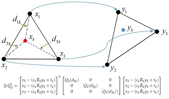
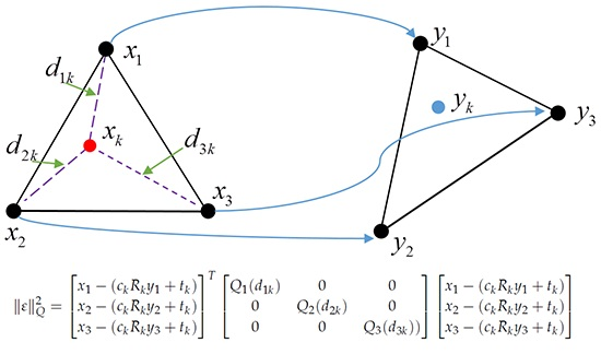
In the simple example illustrated in Figure 1, the red local point should be transformed to obtain the projected blue global point using Equation (7), when given three pairs of GCPs drawn with black points in two coordinate systems. The distances between the red point and the local points of the GCPs are . The distances will make varying contributions to determining the global point .
The objective function of the least squares problem is:
where , a matrix, is a weighting matrix that is a function of the distance and serves as a variable for distance kernel functions. After finding the best similarity transformation parameters , we can perform a similarity transformation to obtain using Equations (7) and (10).
To avoid numerical instability when the iterative solution is adopted for this non-linear solution, data normalization should be required. The normalization matrices of two sets of points in two coordinate systems can be expressed as follows:
where and are the centres of two point sets and and are the covariance of two point sets. Furthermore, the centres and variance can be computed using the following:
After the original points are subject to data normalization, the maximum distance between a point and the centre is . The normalization matrices are applied to two sets of points, and the normalized points are treated as new measurements to estimate the optimal similarity transformation parameters as described by:
Now, the final similarity transformation parameters , with which we can transform , can be computed via multiplication between the normalization matrices and , so that:
3.2. Initialize Similarity Transformation Parameters Using Affine Transformation
To solve the non-linear problem in Equation (9), an affine transformation, which approximates the similarity transformation, will be utilized to provide the initialization. The affine transformation between a pair of points can be defined in the form of the homogeneous vector:
where the matrix A and the vector a consist of twelve affine transformation parameters. To determine the best unknown parameters, Equation (16) can be expressed with another linear equation as a function of affine transformation parameters:
where refers to the elements of the i-th row of matrix A. If more than four pairs of GCPs are available, a linear system can be constructed as follows:
to find the solution of Equation (17); where:
Then, the SVD algorithm can be adopted to solve the linear system:
and the affine transformation parameters can be obtained as:
where:
when the affine transformation parameters are known, the similarity transformation parameters can be calculated via:
4. Distance Kernel Functions
In contrast to the classical method with identity matrices for each measurement, the local points of GCPs should be assigned different weighting matrices as functions of the distances between CPs and these local points. In this study, the weighting matrices will be measured using distance kernel functions; here, the exponential function and Gaussian function are used.
4.1. Exponential Function
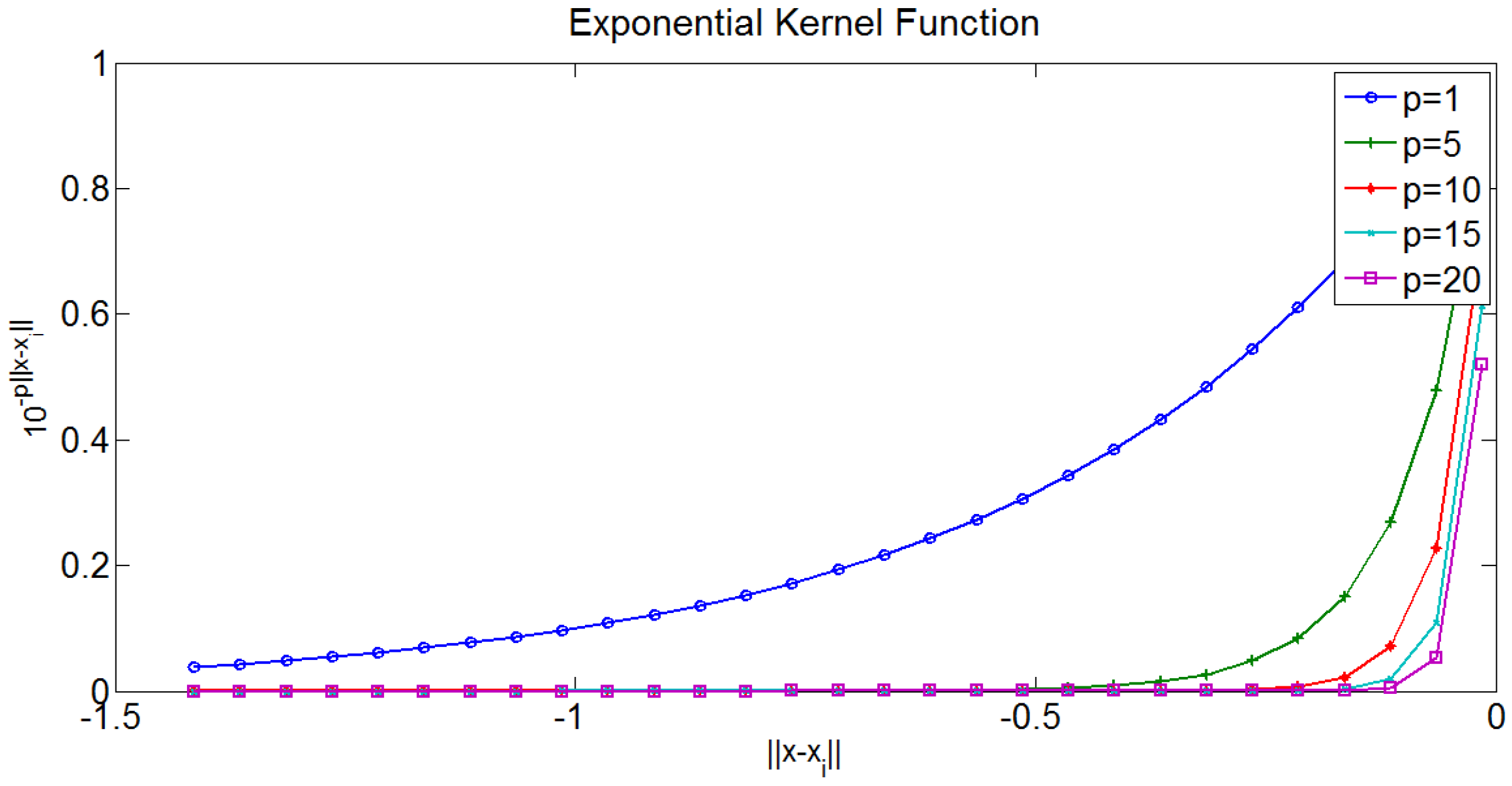
When given a TP must be transformed into the global coordinate system, the weighting matrix of the GCPs can be defined as follows:
where the distance between and is expressed by . Additionally, p controls the gradient of the curve of the exponential function shown in Figure 2, where the five curves of the exponential kernel function are drawn with different colours.
Because all raw points are processed with data normalization, the maximum and minimum distance between two points are and zero, respectively. The weight, computed using the exponential kernel function, ranges from to one, that is . For the maximum weight, when a point to be transformed is located at the position of a GCP, the distance between the two points is zero, that is . In addition, p plays an important role in the distribution of the weight, as well as the minimum weight. If p is large, the minimum weight will be very small, and the gradient of the curve will be very sharp, leading to the ill-conditioning of the least squares in Equation (9). When p is very small, the gradient of the curve is very gentle, and the weights are nearly the same for points with different distances, resulting in poor transformation accuracy. The parameter p is critical to guaranteeing a non-linear least-squares solution with more accuracy of the transformation and better convergence. Thus, we will discuss how the parameter should be set in the Experimental Section.
4.2. Gaussian Function
Similarly, the Gaussian function in Equation (25) is chosen to serve as another type of distance kernel function to compute the weighting matrices as follows:
where determines the minimum weight and the gradient of the Gaussian curve. The five curves are depicted with different colours in Figure 3, where the gradient will become steep when the parameter decreases.
Similarly to the exponential function, the maximum weight of the Gaussian kernel function is one when the point just is located at the position of a GCP, and the minimum weight is . The influence of the accuracy of the absolute orientation affected by this parameter will be thoroughly discussed in Section 5.3.
5. Experiments and Results
In this experiment, six synthetic and two real datasets were utilized to validate and verify the proposed algorithm. First, the six synthetic datasets, whose sizes of the area in the study case range from 20 km × 20 km to 800 km × 100 km, were tested, and we conducted a fair comparison with the classical method. Furthermore, we verified the algorithm using two real datasets to analyse the accuracy obtained using the classical method and the proposed method. Finally, we discussed the influence of two parameters of the distance kernel function on the accuracy using one synthetic datum.
5.1. Synthetic Data
In this section, six synthetic datasets, covering small-scale and large-scale terrains, were designed to validate and analyse the accuracy of the proposed method. To manufacture the two sets of points in the local and global coordinate systems for the absolute orientation problem, we generated the synthetic data using the bundle adjustment (BA) model, as explained in Figure 4. When the terrain size was determined, we randomly generated evenly-distributed GCPs and TPs. In Figure 4, the black points and the red points represent the TPs and the GCPs, respectively. These 3D points can be projected into cameras, forming various image point correspondences. Here, images are captured by a camera that is free of distortion. Additionally, the maximum size of the camera is up to 7680 × 13,824 pixels, and the principal point is located on the centre of the image. The TPs and the GCPs are denoted as and , which are located in the global coordinate system defined as . The image projections of the TPs on the two images involves and , whereas the ones of the GCPs on all visible images consist of and . For the TPs, random Gaussian noise ( pixel) is added to the theoretical image points. Note that no noise is added to the image projections of the GCPs. Serving as the measurements, these image projections will be input into the BA model to triangulate 3D points and orientate cameras in the local coordinate system defined by . Some of these GCPs will be used as the measurements for estimating the similarity transformation parameter, and the remainder will be treated as check points (CPs) to assess the accuracy using the residual mean square error (RMSE).
We manufactured six synthetic datasets, as listed in Table 1, where the area of the study case and the number of images continuously increases. The trajectories of images were designed like a snake shape in the aerial survey [20], in which a downward camera is used. In addition, the forward and side overlaps are up to and , respectively. In Table 1, the numbers of TPs, GCPs and CPs are listed in the fourth, fifth and sixth columns, respectively. In addition, the spatial distribution of GCPs, CPs and 3D TPs of six synthetic datasets is shown in Figure 5, where the terrains are represented with various blue quadrangles using 3D TPs. In addition, the red triangles and yellow circles represent the GCPs and the CPs, respectively.
The GCPs in the sixth column of Table 1 are used to estimate the transformation parameters between two point sets, and the CPs in the seventh column are used to check the accuracy in Table 2. We conducted a fair comparison among the classical absolute orientation method (CAO), the absolute orientation with the exponential kernel function (AO-EF) and the absolute orientation with the Gaussian kernel function (AO-GF). In addition, all results of the absolute orientation method will be compared to another type of method. The method incorporates the GCPs into the BA model in the global coordinate system, yielding better accuracy. We call this technique BA-GCP in this study for convenience. As shown in the fourth column of Table 2, the RMSE of CAO continuously increased with increasing area of the study case. The main reason is that the transformation of the large study case cannot be accurately represented by a set of similarity transformation parameters. However, the accuracies of the two solutions of the proposed method, AO-EF and AO-GF, are very similar and significantly better than those of the CAO. For example, the height RMSE of the AO-EF solution can be reduced to approximately fifty times that of the CAO for the largest dataset. Moreover, the accuracies of the absolute orientation methods, including the classical method and the proposed method, are poorer than those of the BA-GCP method. In contrast to the BA-GCP, which is a direct solution used to triangulate TPs in only one step, the absolute orientation methods first triangulate the local points using a free-net BA model and then perform the 3D transformation. In the first step of the free-net BA, the error will be propagated into the second step, increasing the final error.
Summarizing the above results, the proposed method can significantly improve the accuracy of the absolute orientation, compared to the classical method, regardless of the size of the area of the study case.
5.2. Real Data
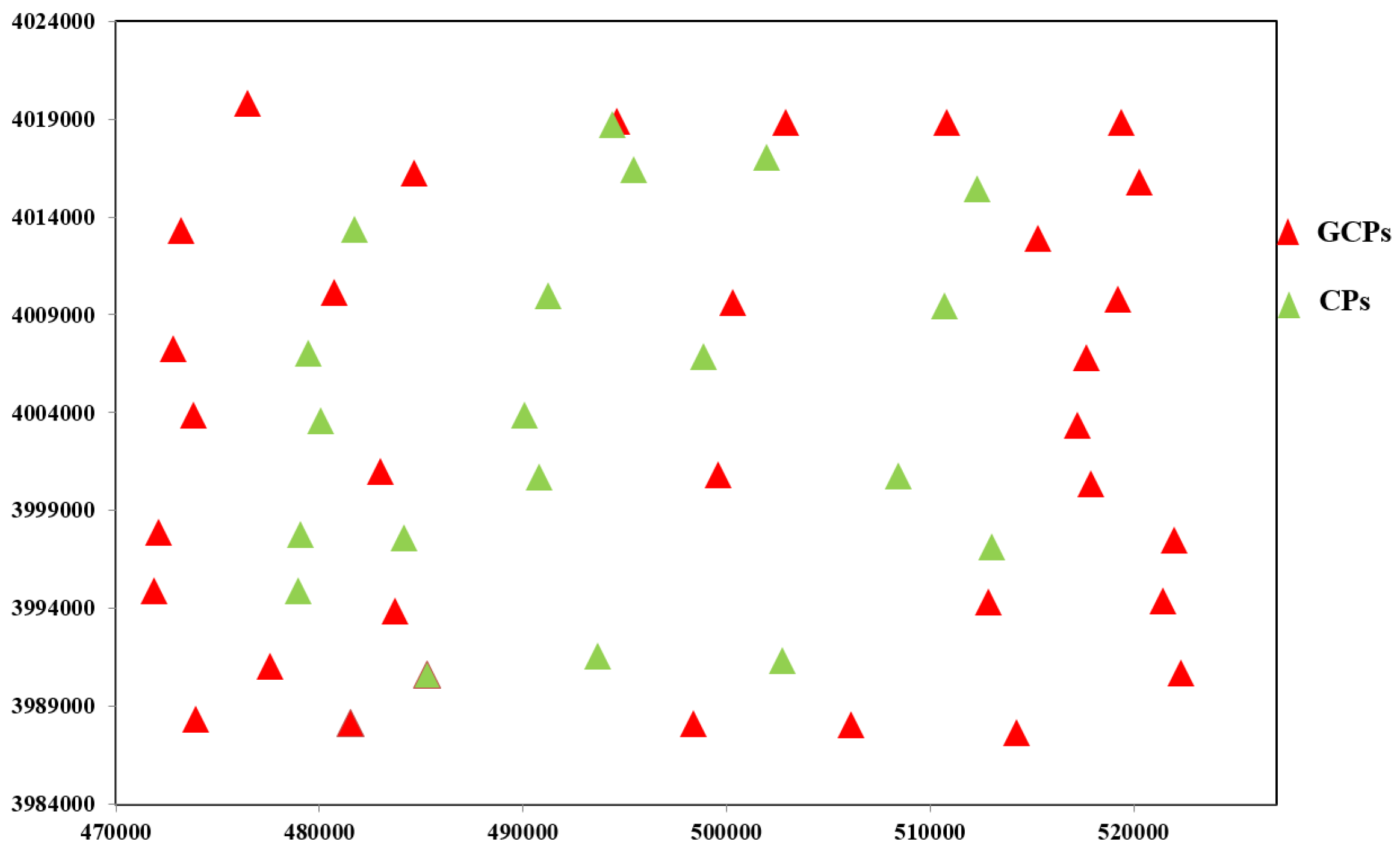
In this section, a small-scale “Village” dataset and a large-scale “Taian” dataset are used to test the proposed algorithm, and the areas of the study cases are up to 2 km × 3.5 km and 53 km × 35 km, respectively. The Village dataset includes imagery of a hilly terrain, and the images with 0.1-m ground sample distances (GSD) are captured by a DMCcamera at a height of 1000 m. The Taian dataset includes imagery of a mountain terrain with 0.5 GSD, and its images are also captured by a DMC camera at a height of 3500 m. Similar to the synthetic datasets, the Village and Taian images were captured by a downward camera and orientated in a snake shape. The forward and side overlaps of the Village dataset are and , while those of the Taian dataset are up to and . In contrast to the synthetic datasets manufactured in Section 5.1, the local points can be triangulated by the BA model using image points generated using feature extraction and a matching algorithm. The L2-SIFT algorithm, which is designed to efficiently extract image point correspondence from large-scale aerial images, is used [20], and ParallaxBA, a type of BA, is utilized to estimate structures and motion [21,22]. The overall parameters of the two real datasets are listed in Table 3. There are six GCPs, six CPs and 90 cameras in the Village dataset, as shown in Figure 6. The GCPs and CPs are denoted by red triangles and green triangles, respectively. In addition, 32 GCPs and 20 CPs of the Taian dataset are evenly distributed in Figure 7, where there are 737 cameras.
For the Village dataset, six GCPs were used to estimate the transformation parameters between two coordinate systems, and the plane and height RMSE are analysed in Table 4 using six CPs. In this table, the RMSE and max residual associated with CAO, AO-EF and AO-GF are compared. The max residuals and the RMSE obtained using the proposed method are slightly better than those obtained using the classical method. The errors of the local points obtained using a free-net BA tested on small study cases are comparatively small and propagated into the global points transformed based on the absolute orientation. For the small-scale aerial photogrammetry, the deformation of point sets in the local and global coordinate systems is relatively small, and the relationship between two coordinate systems can be accurately expressed with the similarity transformation. Thus, the accuracy is slightly improved by the proposed method.
For the Taian dataset, 32 CPs and 20 CPs were used to check the maximum residual and the RMSE obtained by CAO, AO-EF and AO-GF in Table 5, where the accuracies of AO-EF and AO-GF are approximately equal. As shown in the row for the max residual, the height and plane residuals of the proposed method were approximately three-times smaller than those of the classical method. Moreover, the plane RMSE and height RMSE obtained using the proposed method were approximately three- and four-times higher than those of the classical method, and the height RMSE of the proposed method decreased to as low as 3.2 m from the original 12.4 m.
For both the Village and Taian datasets, as in the synthetic datasets, the obtained accuracies using the BA-GCP method are certainly also better than those obtained using the absolute orientation methods. However, the complexity of the absolute orientation method is lower than that of the BA-GCP method, although the accuracy is poorer. More importantly, the absolute orientation method not only is utilized to achieve the TP transformation following the use of the free-net BA using image data, but also performs registration when only 3D points are available.
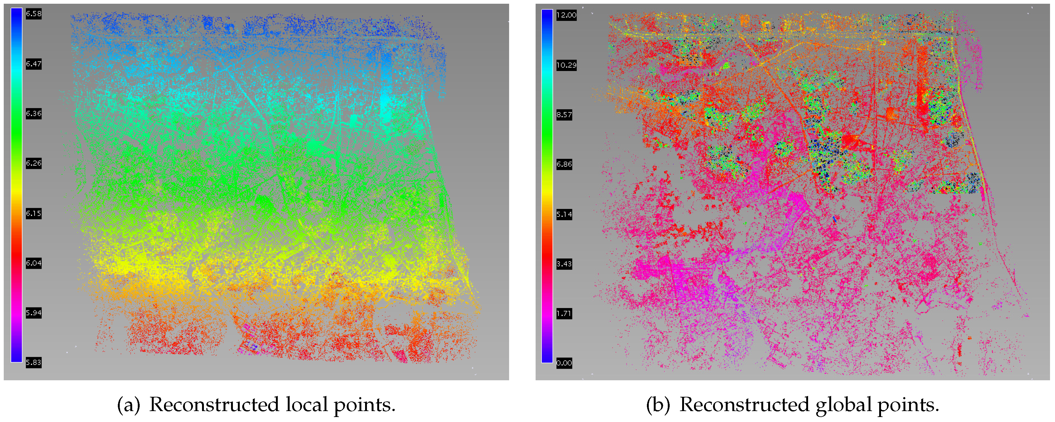
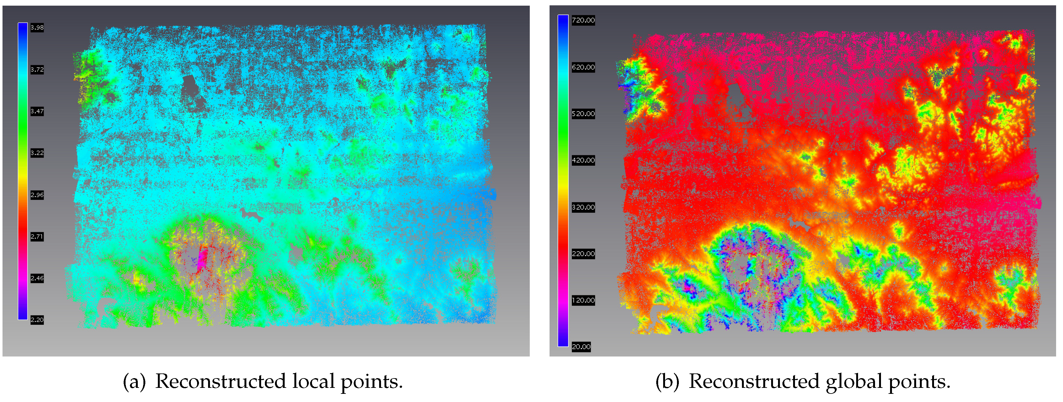
Finally, the transformed TPs located in the global coordinate system using the proposed method are depicted in Figure 8 and Figure 9, and the local TPs are shown in Figure 8a and Figure 9a. The global TPs are drawn in Figure 8b and Figure 9b, and the different elevations of points are shown in different colours. Because there were only slight differences among the TPs transformed using two solutions of the proposed method, we only present the result of the absolute orientation based on the exponential kernel function. From the drawn points, the local points were transformed with high accuracy, and we did not change their structure.
5.3. The Parameters of Distance Kernel Functions
The two parameters, namely those of the exponential kernel function and the Gaussian kernel function, and the distance between the two points affecting the weighting matrices used in the least squares problem are defined in Equation (9). In this study, these two parameters were manually set, and their suggested values are discussed in the experimental analyses as follows. The Sim200-100 synthetic dataset, introduced in Section 5.1, was used to discuss the accuracy variation with these two parameters.
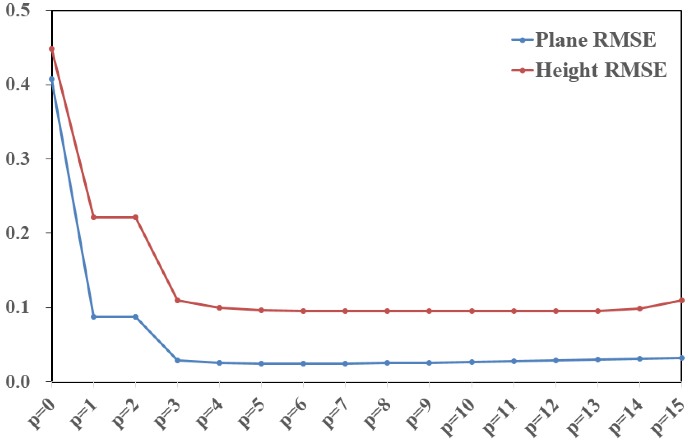
For the exponential kernel function, we set the parameters as . The RMSE and maximum residual of the plane and height are listed in Table 6. Additionally, the RMSE, as a function of the different parameters, is drawn in Figure 10. The plane and height RMSE decreased when the parameters were increased and remained almost constant when pwas set as six. Thus, the parameter of the exponential kernel function was set as six to yield the best results in the experiments.
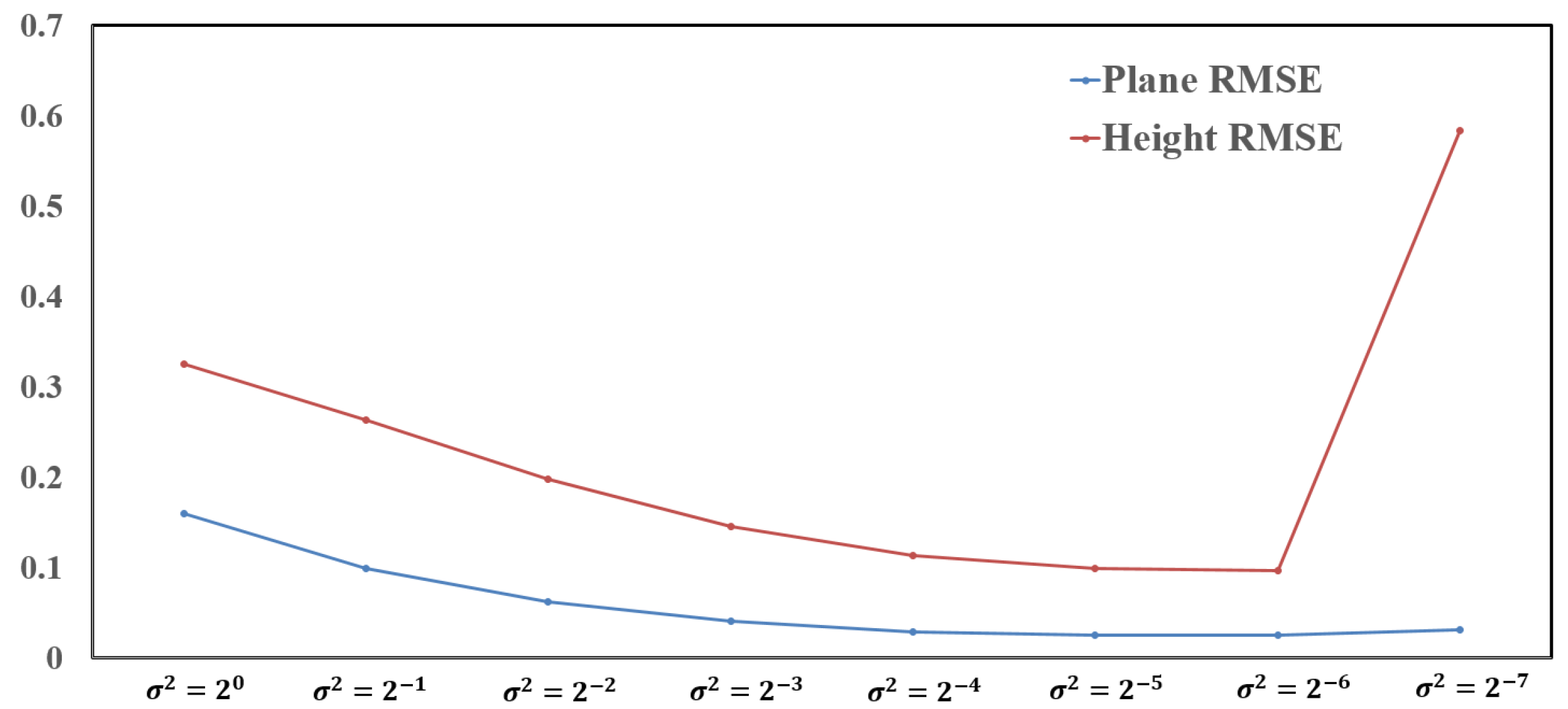
To analyse the parameter of the Gaussian kernel function, we set , and recorded the RMSE and the maximum residual in Table 7, where the plane and height accuracies are listed. In addition, the RMSE, as a function of the parameter, is depicted in Figure 11. The plane and height errors decreased when the parameters ranged from 0 to −7. However, a larger RMSE and larger maximum residual was obtained when , because the effect of the weighting matrices on the distance between points was reduced when was very small. Thus, was found to yield better accuracy in the Gaussian kernel function.
6. Discussion
To improve the accuracy of transformed points, the proposed method represents the transformation of the absolute orientation problem using various sets of similarity transformation parameters instead of only one set. When computing the various sets of parameters, we assign the GCPs with different weighting matrices measured by distance kernel functions.
From the results obtained using synthetic and real datasets analysed in Section 5, it is clearly demonstrated that the accuracies of transformed points obtained using the absolute orientation method are significantly improved by the proposed method compared to the classical method. The extracted image points suffer from noise, which will be propagated into the triangulate points; thus, a 3D reconstructed terrain deforms in the local coordinate system. When the size of a study case area increases, the deformation increases accordingly. For the classical method, the transformation between two coordinate systems is regarded as a rigid-body transformation without deformation, and it is sufficient to represent the transformation using a similarity transformation with seven degrees of freedom. However, the transformation with deformation cannot be accurately expressed using a unique set of similarity transformation parameters by the classical method. The influence of the deformation on the accuracy will be reduced using various sets of similarity transformation parameters in the proposed method, in which the GCPs will be assigned different weighting matrices calculated by distance kernel functions.
The accuracy of the BA-GCP method is higher than that of the classical and proposed absolute orientation methods. This is mainly because the BA-GCP method is a direct solution for triangulating TPs within only one step, whereas the absolute orientation methods first triangulate the local points by a free-net BA model and then perform 3D transformation. For the first step of the free-net BA, the errors of local points will be propagated into the second step, increasing the final error. Although the complexity of the absolute orientation method is lower than that of the BA-GCP method, the accuracies associated with the absolute orientation methods are poorer. Thus, the BA-GCP method is the best method of obtaining a photogrammetric model in the global coordinate system and cannot be substituted by the proposed method for aerial surveys. This study mainly focuses on increasing the accuracy of the classical absolute orientation method. The main deficiency is the higher computational complexity of the proposed method, in which the numerous sets of seven parameters should be computed instead of one set.
7. Conclusions and Future Work
To improve the accuracy of the transformed points obtained using the classical absolute orientation method, a novel method based on distance kernel functions is proposed in this study. The proposed method is able to transform TPs from the local coordinate system to the global one with better accuracy regardless of the size of the study case. In contrast to the classical absolute orientation method, the proposed method represents the transformation using various sets of similarity transformation parameters instead of only one set. For each local TP, a different set of parameters is estimated by a least squares solution, in which GCPs are assigned different weighting matrices measured by distance kernel functions. In this study, the exponential function and Gaussian function are used. Although a higher computational cost is required, the proposed method can significantly improve the accuracy of transformed points, especially for large-scale study cases, as demonstrated by its application to the six synthetic and two real datasets. Thus, the proposed method represents a feasible solution for obtaining more accurate transformed points using the absolute orientation method in the field of photogrammetry.
In future, we will focus on determining robust parameters for the exponential and Gaussian distance kernel function.
Acknowledgments
This work is supported by the National Natural Science Foundation of China (Grant Numbers 41431179 and 41571432) and the Guangxi Natural Science Foundation with Grant Number 2015GXNSFDA139032. Finally, the authors would like to sincerely thank the editor and anonymous reviewers. Due to their patience, the quality of the paper was greatly improved.
Author Contributions
Yanbiao Sun, Liang Zhao and Guoqing Zhou conceived of and designed the experiments. Yanbiao Sun performed the experiments. Lei Yan and Guoqing Zhou analysed the data. Yanbiao Sun wrote the paper.
Conflicts of Interest
The authors declare no conflict of interest.
References
- Dowman, I.J. Automating image registration and absolute orientation: Solutions and problems. Photogramm. Rec. 1998, 16, 5–18. [Google Scholar] [CrossRef]
- Garcia-Gago, J.; Gonzalez-Aguilera, D.; Gomez-Lahoz, J.; San Jose-Alonso, J.I. A photogrammetric and computer vision-based approach for automated 3D architectural modeling and its typological analysis. Remote Sens. 2014, 6, 5671–5691. [Google Scholar] [CrossRef]
- Johnson, A.E.; Hebert, M. Surface registration by matching oriented points. In Proceedings of the International Conference on Recent Advances in 3-D Digital Imaging and Modeling, Washington, DC, USA, 12 May 1997; pp. 121–128.
- Remondino, F. Heritage recording and 3D modeling with photogrammetry and 3D scanning. Remote Sens. 2011, 3, 1104–1138. [Google Scholar] [CrossRef] [Green Version]
- Sharp, G.C.; Lee, S.W.; Wehe, D.K. ICP registration using invariant features. IEEE Trans. Pattern Anal. Mach. Intell. 2002, 24, 90–102. [Google Scholar] [CrossRef]
- Tommaselli, A.M.; Galo, M.; De Moraes, M.V.; Marcato, J.; Caldeira, C.R.; Lopes, R.F. Generating virtual images from oblique frames. Remote Sens. 2013, 5, 1875–1893. [Google Scholar] [CrossRef]
- Xu, Z.; Wu, L.; Shen, Y.; Li, F.; Wang, Q.; Wang, R. Tridimensional reconstruction applied to cultural heritage with the use of camera-equipped UAV and terrestrial laser scanner. Remote Sens. 2014, 6, 10413–10434. [Google Scholar] [CrossRef]
- Blostein, S.D.; Huang, T.S. Estimating 3-D motion from range data. In Proceedings of the Artificial Intelligence Applications, Denver, CO, USA, 5 December 1984; pp. 246–250.
- Wolf, P.R. Solutions Manual to Accompany Elements of Photogrammetry: With Air Photo Interpretation and Remote Sensing; McGraw-Hill: New York, NY, USA, 1983. [Google Scholar]
- Slama, C.C.; Theurer, C.; Henriksen, S.W. Manual of Photogrammetry, 4th ed.; American Society for Photogrammetry and Remote Sensing: Bethesda, MD, USA, 1980. [Google Scholar]
- Awange, J.L.; Grafarend, E. Polynomial optimization of the 7-parameter datum transformation problem when only three stations in both systems are given. Zeitschrift fuer Vermessungswesen 2003, 127, 109–117. [Google Scholar]
- Thompson, E.H. An exact linear solution of the problem of absolute orientation. Photogrammetria 1959, 15, 163–179. [Google Scholar] [CrossRef]
- Horn, B.K. Closed-form solution of absolute orientation using unit quaternions. J. Opt. Soc. Am. A 1987, 4, 629–642. [Google Scholar] [CrossRef]
- Horn, B.K.; Hilden, H.M.; Negahdaripour, S. Closed-form solution of absolute orientation using orthonormal matrices. J. Opt. Soc. Am. A 1998, 5, 1127–1135. [Google Scholar] [CrossRef]
- Arun, K.S.; Huang, T.S.; Blostein, S.D. Least-squares fitting of two 3-D point sets. IEEE Trans. Pattern Anal. Mach. Intell. 1987, 5, 698–700. [Google Scholar] [CrossRef]
- Umeyama, S. Least-squares estimation of transformation parameters between two point patterns. IEEE Trans. Pattern Anal. Mach. Intell. 1991, 13, 376–380. [Google Scholar] [CrossRef]
- Mohamed, A.; Wilkinson, B. Direct georeferencing of stationary LiDAR. Remote Sens. 2009, 1, 1321–1337. [Google Scholar] [CrossRef]
- Alba, M.I.; Barazzetti, L.; Scaioni, M.; Rosina, E.; Previtali, M. Mapping infrared data on terrestrial laser scanning 3D models of buildings. Remote Sens. 2011, 3, 1847–1870. [Google Scholar] [CrossRef]
- Hashemi, A.; Kalantari, M.; Kasser, M. Direct Solution of the 7 parameters transformation problem. Appl. Math. 2013, 7, 1375–1382. [Google Scholar] [CrossRef]
- Sun, Y.; Zhao, L.; Huang, S.; Yan, L.; Dissanayake, G. L2-sift: Sift feature extraction and matching for large images in large-scale aerial photogrammetry. ISPRS J. Photogramm. Remote Sens. 2014, 91, 1–16. [Google Scholar] [CrossRef]
- Zhao, L.; Huang, S.; Yan, L.; Dissanayake, G. Parallax angle parametrization for monocular SLAM. In Proceedings of the IEEE International Conference on Robotics and Automation (ICRA), Shanghai, China, 9 May 2011; pp. 3117–3124.
- Zhao, L.; Huang, S.; Sun, Y.; Yan, L.; Dissanayake, G. Parallaxba: Bundle adjustment using parallax angle feature parametrization. Int. J. Robot. Res. 2015, 34, 493–516. [Google Scholar] [CrossRef]
Figure 1.
A simple example using three pairs of ground control points (GCPs) to compute the optimal set of transformation parameters for tie points (TPs).
Figure 1.
A simple example using three pairs of ground control points (GCPs) to compute the optimal set of transformation parameters for tie points (TPs).
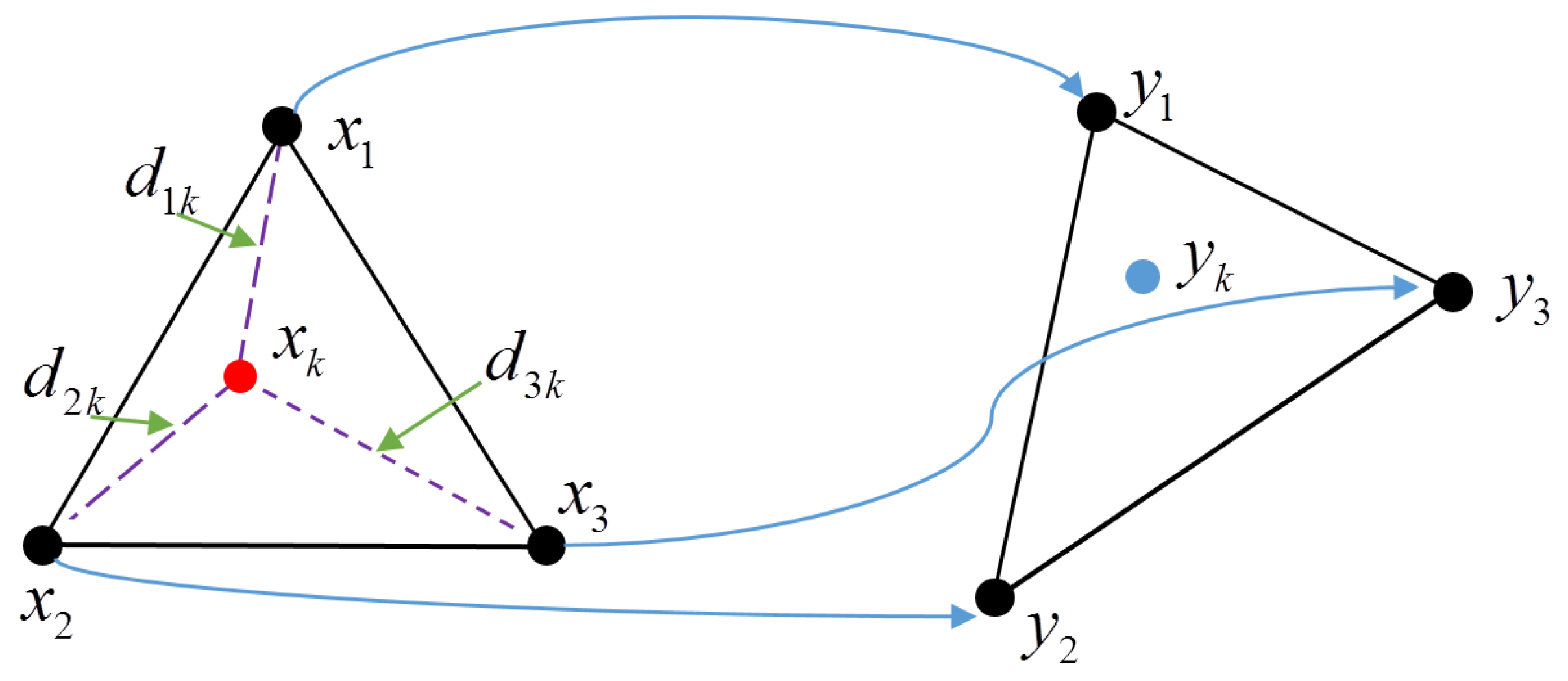
Figure 2.
Exponential kernel function.

Figure 3.
Gaussian kernel function.
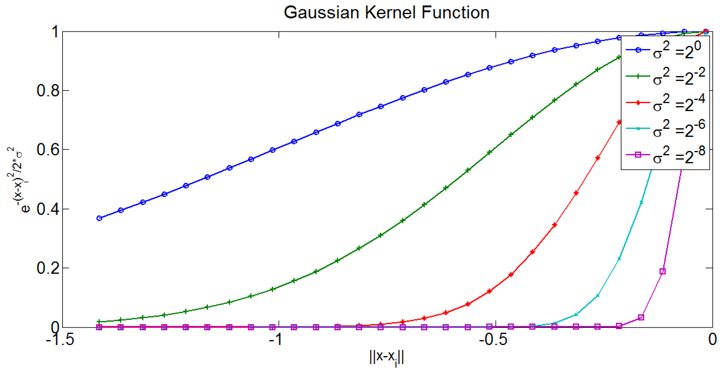
Figure 4.
The workflow of manufacturing two point sets of synthetic data using the bundle adjustment (BA) model.
Figure 4.
The workflow of manufacturing two point sets of synthetic data using the bundle adjustment (BA) model.

Figure 5.
The spatial distribution of GCPs, CPs and 3D tie points of six synthetic datasets. The red triangles and yellow circles represent GCPs and CPs, respectively. Additionally, TPs are drawn with blue quadrangles. (a), (b), (c), (d), (e) and (f) represent the spatial distribution of Sim20-20, Sim50-50, Sim100-100, Sim200-100, Sim400-100 and Sim800-100 datasets, respectively.
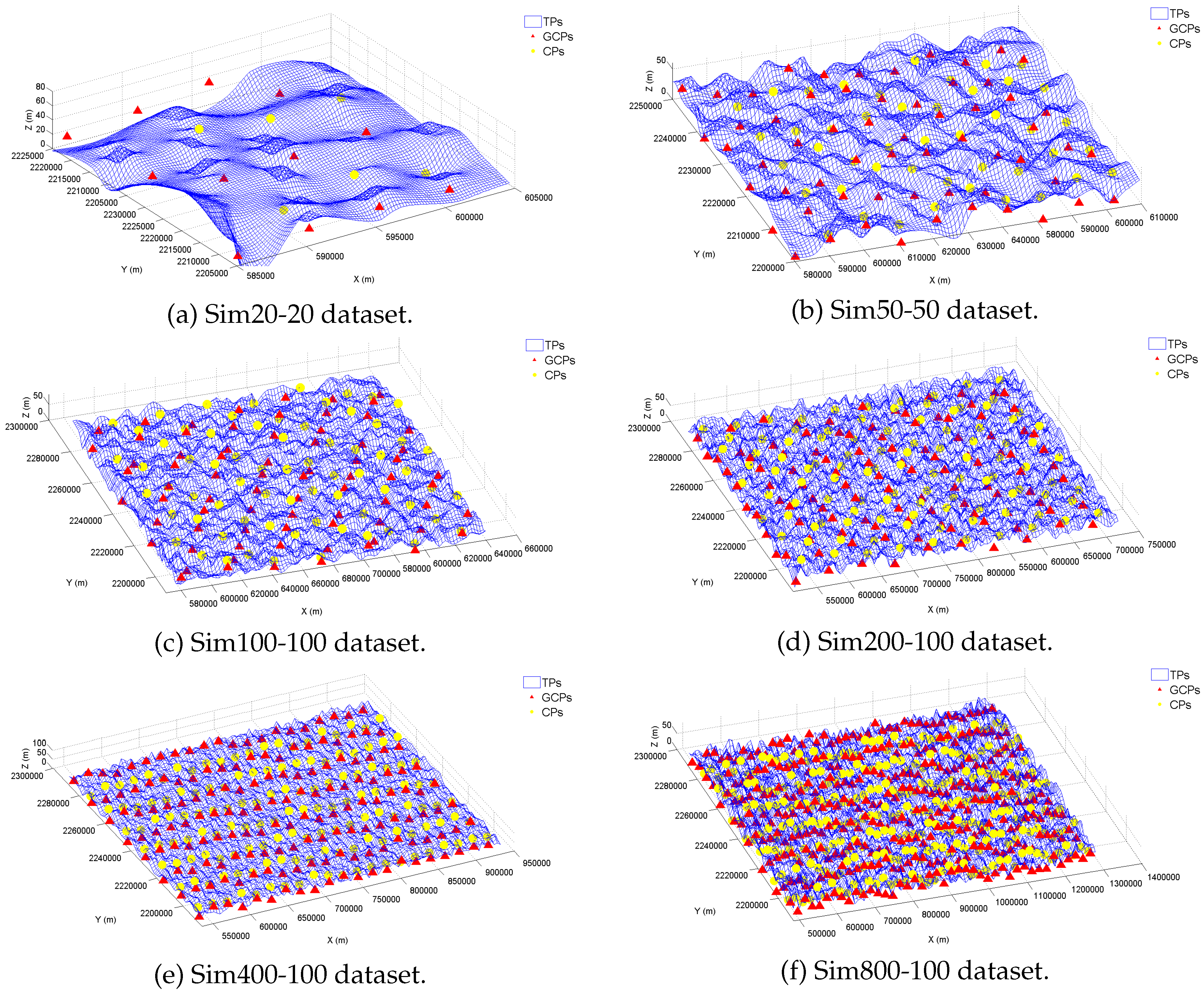
Figure 6.
Distribution of the GCPs and CPs for the Village data.
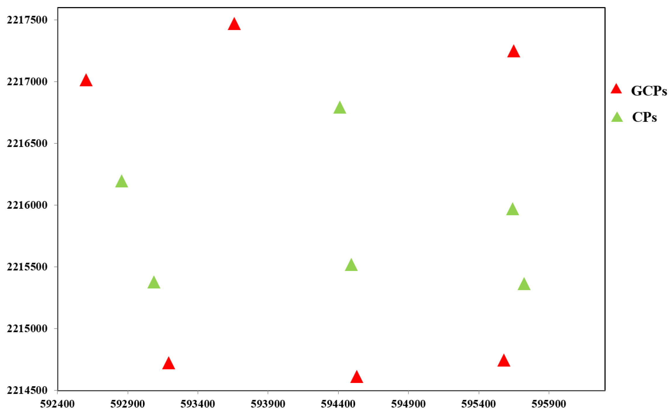
Figure 7.
Distribution of the GCPs and CPs for the Taian data.

Figure 8.
Reconstructed 3D terrain of the Village dataset in the local and global coordinate systems. The unit of measure of the reconstructed points in the global coordinate system is meters, whereas the local points have no practical meaning due to a lack of scale and origin information. (a) and (b) are 3D triangulated points of the Village dataset in the local and global coordinate systems, respectively.

Figure 9.
Reconstructed 3D terrain of the Taian dataset in the local and global coordinate systems. The unit of measure of the reconstructed points in the global coordinate system is meters, whereas the local points have no practical meaning due to a lack of scale and origin information. (a) and (b) are 3D triangulated points of the Taian dataset in the local and global coordinate systems, respectively.

Figure 10.
The RMSE as a function of the different parameters in the exponential kernel function.

Figure 11.
The RMSE as a function of the different parameters in the Gaussian kernel function.


| Data | Area | Images | Tie Points | GCPs | CPs |
|---|---|---|---|---|---|
| Sim20-20 | 20 km × 20 km | 80 | 1585 | 12 | 6 |
| Sim50-50 | 50 km × 50 km | 440 | 10,320 | 60 | 55 |
| Sim100-100 | 100 km × 100 km | 1738 | 42,422 | 74 | 69 |
| Sim200-100 | 200 km × 100 km | 3453 | 84,045 | 110 | 105 |
| Sim400-100 | 400 km × 100 km | 6886 | 167,712 | 168 | 147 |
| Sim800-100 | 800 km × 100 km | 13,772 | 335,268 | 336 | 294 |
Table 2.
The plane and height RMSE obtained using the classical method and the proposed method. CAO, classical absolute orientation; AO-EF, absolute orientation with the exponential kernel function; GF, Gaussian kernel function.
| RMSE (m) | BA-GCP | CAO | Proposed AO-EF | Proposed AO-GF | |
|---|---|---|---|---|---|
| Sim20-20 | Plane | 0.0056 | 0.0286 | 0.0136 | 0.0145 |
| Height | 0.00625 | 0.1269 | 0.0866 | 0.0863 | |
| Sim50-50 | Plane | 0.0067 | 0.0503 | 0.0112 | 0.0106 |
| Height | 0.0385 | 0.1356 | 0.0495 | 0.0494 | |
| Sim100-100 | Plane | 0.0080 | 0.0791 | 0.0125 | 0.0134 |
| Height | 0.0448 | 0.2251 | 0.0511 | 0.0552 | |
| Sim200-100 | Plane | 0.0112 | 0.4078 | 0.0255 | 0.0248 |
| Height | 0.0867 | 0.4477 | 0.0951 | 0.0990 | |
| Sim400-100 | Plane | 0.0096 | 0.3456 | 0.0184 | 0.0243 |
| Height | 0.0700 | 1.2799 | 0.0932 | 0.1339 | |
| Sim800-100 | Plane | 0.0098 | 1.2407 | 0.0239 | 0.0665 |
| Height | 0.0772 | 7.4464 | 0.1399 | 0.2939 |
| Data | Area | Images | TPs | GCPs | CPs |
|---|---|---|---|---|---|
| Village | 2 km × 3.5 km | 90 | 305,719 | 6 | 6 |
| Taian | 53 km × 35 km | 737 | 2,743,625 | 32 | 20 |
Table 4.
The plane and height RMSE of the Village dataset obtained by the classical method and the proposed method.
| Parameter | BA-GCP | CAO | Proposed AO-EF | Proposed AO-GF | |
|---|---|---|---|---|---|
| Max residual (m) | East | 0.1361 | 0.1307 | 0.0999 | 0.1091 |
| North | 0.2347 | 0.1775 | 0.1968 | 0.2001 | |
| Plane | 0.1779 | 0.2068 | 0.2143 | 0.2189 | |
| Height | 0.3185 | 0.4147 | 0.2959 | 0.3253 | |
| RMSE (m) | East | 0.0707 | 0.0797 | 0.0635 | 0.0658 |
| North | 0.1370 | 0.0967 | 0.1046 | 0.1033 | |
| Plane | 0.1090 | 0.1253 | 0.1224 | 0.1224 | |
| Height | 0.1800 | 0.2541 | 0.2287 | 0.2320 | |
Table 5.
The plane and height RMSE of the Taian dataset obtained by the classical method and the proposed method.
| Parameter | BA-GCP | CAO | Proposed AO-EF | Proposed AO-GF | |
|---|---|---|---|---|---|
| Max residual (m) | East | 0.6881 | 1.7903 | 0.5742 | 0.5606 |
| North | 1.0715 | 2.5271 | 0.7532 | 0.6710 | |
| Plane | 0.7579 | 2.5284 | 0.7989 | 0.7585 | |
| Height | 3.6663 | 21.2717 | 7.6978 | 7.4669 | |
| RMSE (m) | East | 0.2507 | 0.6500 | 0.2312 | 0.2313 |
| North | 0.3923 | 0.9734 | 0.3177 | 0.3039 | |
| Plane | 0.3292 | 1.1705 | 0.3929 | 0.3819 | |
| Height | 1.2780 | 12.4855 | 3.2782 | 3.2696 | |
Table 6.
The RMSE and max residual of the plane and height directions as a function of the parameters in the exponential kernel function.
| RMSE (m) | Max Residual (m) | |||
|---|---|---|---|---|
| Plane | Height | Plane | Height | |
| 0.4078 | 0.4477 | 1.0732 | 1.1884 | |
| 0.0877 | 0.2217 | 0.3525 | 0.6538 | |
| 0.0877 | 0.2217 | 0.3525 | 0.6538 | |
| 0.0295 | 0.1094 | 0.1360 | 0.3425 | |
| 0.0262 | 0.1003 | 0.1113 | 0.3024 | |
| 0.0252 | 0.0971 | 0.1000 | 0.2923 | |
| 0.0249 | 0.0958 | 0.0949 | 0.2871 | |
| 0.0251 | 0.0953 | 0.0925 | 0.2842 | |
| 0.0255 | 0.0951 | 0.0961 | 0.2825 | |
| 0.0262 | 0.0950 | 0.1057 | 0.2821 | |
| 0.0271 | 0.0949 | 0.1160 | 0.2834 | |
| 0.0282 | 0.0949 | 0.1264 | 0.2845 | |
| 0.0293 | 0.0950 | 0.1362 | 0.2852 | |
| 0.0303 | 0.0959 | 0.1448 | 0.2858 | |
| 0.0312 | 0.0992 | 0.1520 | 0.3011 | |
| 0.0320 | 0.1098 | 0.1578 | 0.4331 | |
Table 7.
The RMSE and maximum residual of the plane and height directions obtained using different parameters in the Gaussian kernel function.
| RMSE (m) | Max Residual (m) | |||
|---|---|---|---|---|
| Plane | Height | Plane | Height | |
| 0.1589 | 0.3243 | 0.5063 | 0.8495 | |
| 0.0982 | 0.2630 | 0.3645 | 0.7273 | |
| 0.0616 | 0.1973 | 0.2604 | 0.5867 | |
| 0.0407 | 0.1449 | 0.1857 | 0.4574 | |
| 0.0288 | 0.1127 | 0.1274 | 0.3526 | |
| 0.0248 | 0.0990 | 0.0947 | 0.2978 | |
| 0.0251 | 0.0963 | 0.0896 | 0.2843 | |
| 0.0312 | 0.5833 | 0.1498 | 3.5668 | |
© 2016 by the authors; licensee MDPI, Basel, Switzerland. This article is an open access article distributed under the terms and conditions of the Creative Commons by Attribution (CC-BY) license (http://creativecommons.org/licenses/by/4.0/).
Share and Cite
MDPI and ACS Style
Sun, Y.; Zhao, L.; Zhou, G.; Yan, L. Absolute Orientation Based on Distance Kernel Functions. Remote Sens. 2016, 8, 213. https://doi.org/10.3390/rs8030213
AMA Style
Sun Y, Zhao L, Zhou G, Yan L. Absolute Orientation Based on Distance Kernel Functions. Remote Sensing. 2016; 8(3):213. https://doi.org/10.3390/rs8030213
Chicago/Turabian StyleSun, Yanbiao, Liang Zhao, Guoqing Zhou, and Lei Yan. 2016. "Absolute Orientation Based on Distance Kernel Functions" Remote Sensing 8, no. 3: 213. https://doi.org/10.3390/rs8030213
Note that from the first issue of 2016, this journal uses article numbers instead of page numbers. See further details here.