1. Introduction
The Earth’s surface has been experiencing intensive tree cover loss and gain [
1]. Tree cover change has a significant influence on environmental change, including global warming, carbon sequestration, hydrology regulation, ecosystem disturbance and soil erosion [
2,
3,
4]. It also has crucial social impacts on food security, outdoor recreation, local economy and social stability. The intensified forest tree cover change and its prominent environmental and social impacts necessitate the monitoring and identification of its drivers. A large and growing body of literature focuses on exploring factors of tree cover loss [
5,
6,
7,
8,
9,
10,
11], while factors of tree cover gain have received much less attention [
12,
13,
14]. Even fewer studies have investigated tree cover loss and gain simultaneously [
2]. Furthermore, the scale of analysis is closely related to which aspects of tree cover loss and/or gain are analyzed,
i.e., the quantity and location issue [
6]. Most studies were conducted at the regional or global scale, with the mapping unit of analysis being continents [
5] or administrative units, such as country [
7,
15] and municipality [
2]. These studies are usually limited to the quantity issue: how are the rate and extent of tree cover change influenced by different factors? The location issue focuses on exploring factors that determine where the tree cover change may occur. The explanation of the location issue is still unsatisfactory. Because the physical and social environments vary, important factors of tree cover loss and gain may be different among regions and across time. Even the same factor may function distinctively [
16,
17,
18,
19,
20]. The spatio-temporal variation is only partly recognized and rarely addressed in the literature. Identification of underlying factors that influence the location of tree cover loss and gain and the examination of their spatio-temporally-variant importance are of utmost importance for more effective and sustainable forest management practices and the development of future forestry policies.
The major factors of tree cover loss and gain include socioeconomic factors, institutional factors, biophysical factors, proximity to infrastructure and initial landscape patterns [
2,
4,
12,
21,
22,
23,
24,
25]. Socioeconomic and institutional factors tackle the quantity issue. They actually “drive” the tree cover change by creating land change pressures and, therefore, can also be referred to as socioeconomic and institutional drivers. The biophysical, proximity to infrastructure and initial landscape pattern factors, on the other hand, are not drivers of tree cover change. Their spatial variability influence the location preference of tree cover and determine collectively at the local level where the tree cover change may occur (
i.e., the location issue) [
26].
Biophysical factors, such as topography and soil type, determine the suitability of a location for tree growth. Fertile soils, low lying zones, flat and gently-sloping areas generally characterize regions of tree cover loss [
4,
16,
27,
28]. This can be attributed to the suitability of these regions for agriculture and grazing, leading to a high probability of them being lost to cropland or pastures [
22,
24]. Similarly, the concentration of agriculture in these regions makes tree cover gain more likely to occur in marginal, abandoned agricultural areas [
29]. More emphasis has recently been put on proximity to infrastructure factors [
26]. Many studies have demonstrated the importance of proximity factors in tree cover change. For example, tree cover loss tends to occur along major transportation networks [
26,
30]; proximity to settlements generally tends to reduce the tree cover loss probability [
27]. Though less considered, initial landscape pattern factors, such as the initial land cover, initial landscape pattern in the vicinity and distances to patches of different land cover types are also critical for tree cover change [
4,
21,
27,
31].
This paper focuses on pinpointing factors influencing tree cover loss and gain probabilities at the pixel level and on evaluating the heterogeneous importance of factors in two periods of 1991 through 2002 and 2002 through 2013 and in four different counties within the Li River Basin (LRB), Guangxi Zhuang Autonomous Region, China. Since this paper intends to address the location issue rather than the quantity issue, the biophysical, proximity to infrastructure and initial landscape pattern factors were considered. Remote sensing has been successfully used in the studies exploring factors of tree cover change [
6,
22,
32,
33,
34]. It is a cost-effective means to provide wall-to-wall information on land cover change over a large region and, therefore, is superior to ground-based investigation in broad-scale tree cover change studies. In this paper, Landsat images in combination with other ancillary spatially-explicit data were used to generate land cover classification images and three types of factors, including biophysical, proximity to infrastructure and initial landscape pattern factors. The random forests modeling technique [
35] can generate an estimate of the relative importance of independent variables and can deal with a large number of independent variables and large datasets with a high efficiency [
36]. These advantages make random forests a suitable modeling approach to be used in this paper. Models were built for the four counties within the LRB, for the two periods and for the complete pooled dataset. A factor importance ranking and a set of important factors were derived for each model. The partial dependence plots were generated for the most important factors to reveal how tree cover loss and gain probabilities change with these factors. These further our understanding of how factors of tree cover loss and gain and their importance vary by region and period at the pixel level.
2. Materials and Methods
2.1. Study Area
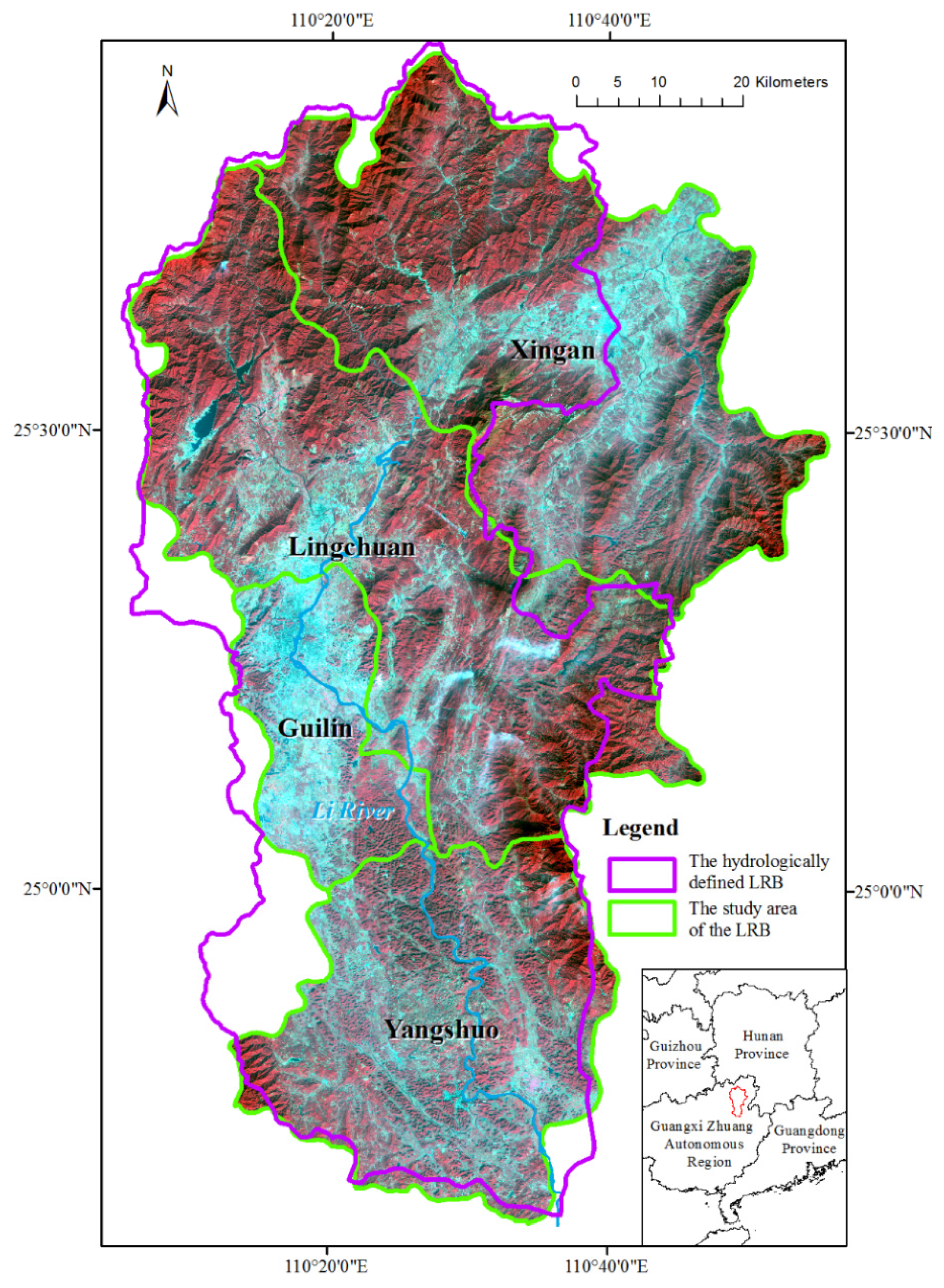
In lieu of the hydrologically-defined Li River Basin, this paper uses an area encompassing the four counties of Guilin Municipal District (GL), Lingchuan County (LC), Xing’an County (XA) and Yangshuo County (YS) as the study area, referred to as the Li River Basin (LRB) (
Figure 1). This is to facilitate the investigation of how the influence of potential factors on tree cover change varies across counties.
The LRB is located in the northeastern Guangxi Zhuang Autonomous Region, China. The climate is mainly a sub-tropical monsoon climate with the dry season in September to February and the wet season in March to August. It has highly complex topography consisting of steep mountains and floodplains. The LRB is also well known for its unique karst landscape. Originating from Mao’er Mountain in Xing’an County, the Li River meets with the Gantang River, Taohua River, Yulong River and Jinbao River, and as such, it flows south to become the Gui River. The Li River and its tributaries formed the advanced river system within the LRB. The well-developed transportation infrastructure includes three national roads, three provincial roads, the Guilin Liangjiang International Airport and the Hunan-Guangxi Railway, providing connections to local tourism destinations.
Guilin, as the most developed and fastest growing county within the LRB, has the lowest tree coverage, much more dynamic tree cover change and the most advanced transportation network. Lingchuan is immediately northeast of Guilin and functions as the suburban expansion of Guilin to deal with the issue associated with the saturated urbanization level of Guiling. Xing’an has Mao’er Mountain, the highest peak in southern China, and is the origin of many rivers. Both Lingchuan and Xing’an are abundant with dense native tree cover mostly distributed on the steep mountains and, therefore, have many natural reserves, featuring the Qingshitan Origin Reserve in Lingchuan and the Mao’er Mountain reserve in Xingan. Yangshuo has been a popular resort destination since the 1980s with a rapid growth in service industries. It is of great interest to assess the influence of three categories of factors on tree cover change in the four counties with distinctive characteristics across time within the period of 1991 through 2013 addressed in this paper.
2.2. Generation of the Dependent Variable
The study area of the LRB is covered by four scenes of Landsat images. A total of 12 geometrically-corrected and geo-referenced scenes of Landsat images for the years of 1991, 2002 and 2013 were downloaded from the Earth Resources Observation and Science (EROS) Center, United States Geological Survey (USGS).
Table S1 shows the acquisition time, sensor and processing level of each scene. The scenes were mostly acquired in the dry season with either no or very sparse cloud cover. The radiometric calibration module of the Environment for Visualizing Images software (ENVI, Version 5.1) was used to conduct the radiometric calibration. The scenes were further atmospherically corrected using the dark object subtraction (DOS) method [
37]. Each scene was also orthorectified using a 1:50,000 topographical map to enable more accurate tree cover change detection across time. The harvested cropland, degraded rangeland and barren land in the dry season have similar spectral property and are not able to be distinguished accurately. Since this paper focuses on tree cover change, the 12 scenes were classified into tree cover, water, urban, other land cover and cloud/shadow using an object-oriented algorithm implemented by eCognition 8.7. The cloud/shadow pixels were excluded from the following analysis. The accuracy of the land cover classification image of 2013 was assessed via ground-truthing and photointerpretation of high resolution Google Earth (GE) images [
38,
39]. A total number of 100 ground points were randomly selected in the vicinity of major roads, and the land cover types of 69 were able to be identified via field visits in October 2013. Another 500 points were obtained using stratified random sampling, and the land cover types of 470 were able to be identified via photointerpretation of GE images. GE images were acquired in 2013 by SPOT, GeoEye and WorldView, with a horizontal accuracy of 39.7 meters [
40]. The ground information was not available for the other two historical images. The accuracy assessment of these images was conducted via the county-level land use maps, field interviews, yearbooks and historical documents. The overall accuracies of the three images are all over 88%.
Table S2 shows the confusion matrices for the three land cover classification images.
The dependent variable was generated as a categorical variable for each period. The two land cover classification images associated with each period were used to re-categorize each pixel into four types: (1) tree cover loss pixels: the pixels that were initially tree cover and converted to non-tree-cover during the corresponding period; (2) tree cover gain pixels: the pixels that were initially non-tree-cover and converted to tree cover during the corresponding period; (3) remain tree-covered pixels: the pixels that remain tree covered during the corresponding period; (4) other pixels: the pixels that remain non-tree covered during the corresponding period.
Figure S1 presents the areas of tree cover loss and gain.
2.3. Generation of Potential Factors
The potential factors collectively determine the probability of a pixel to experience tree cover loss and gain.
Table 1 shows a complete list of potential factors, including the initial landscape pattern, biophysical and proximity factors.
2.3.1. Initial Landscape Pattern Factors
The initial landscape pattern factors include the initial land cover, initial landscape pattern in the vicinity, and distance to patches of different land cover types. The initial landscape pattern factors were calculated for two types of neighborhood: the immediate neighbors (the eight surrounding pixels) and the round neighborhood with a radius of 200 meters. Land cover consistency and heterogeneity focus on the immediate neighbors. Land cover consistency is the number of pixels that are of the same land cover type with the focal pixel, and land cover heterogeneity is the number of land cover types in the eight surrounding pixels. The land cover majority and variety, edge density, and percentage of landscape are calculated for the round neighborhood. The land cover majority and variety are respectively the majority of and the number of land cover types within the neighborhood. Edge density and percentage of landscape are two important landscape pattern metrics calculated using Fragstats 4.2 [
41]. Landscape pattern metrics are patch-based algorithms. A patch is a contiguous area composed of pixels of the same land cover type [
42]. Spatial patterns of patches, classes of patches and entire landscapes are quantified to acquire patch-level, class-level and landscape-level metrics, respectively. Edge density was calculated at the landscape level, describing landscape fragmentation in the neighborhood:
where
is edge density,
is the total length of edge in landscape and
is the total landscape area. The percentage of landscape is an indicator of the landscape composition and was calculated as:
where
is the percentage of the landscape occupied by land cover type
,
is area of the
j-th patch of land cover type
and
is the total landscape area. Distances to patches were calculated as the distances to the closest patch of each land cover type and took the value of zero when the focal pixel was within the patch.
2.3.2. Biophysical Factors
Biophysical factors include topographic factors, soil type and climatic factors. Topographic factors, including elevation, slope, aspect and geomorphological complexity, were generated from the ASTER Global Digital Elevation Model Version 1 released in 2009 by a collaboration of The Ministry of Economy, Trade and Industry (METI) of Japan and the United States National Aeronautics and Space Administration (NASA). SLOPE was organized into a six-level ordinal variable using the break points of 2°, 5°, 10°, 20° and 30°. ASPECT was a categorical variable with its possible values being north-, south-, east- and west-facing, as well as undefined when the slope gradient is less than 2°. Geomorphological complexity (GEOM) was calculated as the standard deviation of elevation in the neighborhood with a radius of 200 meters. Soil type was derived from the Harmonized World Soil Database (HWSD) [
43]. Climatic factors include annual mean temperature, annual precipitation and the standard deviations of monthly temperature and precipitation, describing the average and seasonal variation of temperature and precipitation. The four climatic factors were calculated from the WorldClim dataset representative of the climatic conditions of 1950 to 2000 with a spatial resolution of 30 arc-seconds [
44]. These factors were resampled to 30 meters to be compatible with Landsat data.
2.3.3. Proximity Factors
Proximity factors of the period 1991 to 2002 and 2002 to 2013 were calculated using the vector data of 2002 and 2013, respectively. The vector data of 2002 were acquired from the National Fundamental Geographic Information System (NFGIS) database produced by the State Bureau of Surveying and Mapping of China. The vector data of 2013 were acquired by updating the 2002 vector data using the OpenStreetMap dataset and yearbooks. The proximity factors include both distance factors and density factors. Distance factors include distances to all roads regardless of their types and to four types of roads, including national roads, provincial roads, county roads and highways, as well as distances to railways, attractions, public transportation stations and settlements. The kernel densities of settlements and roads were generated for the neighborhood with a search radius of 6 km.
2.4. Sampling
Spatial autocorrelation is a major concern of many statistical analysis techniques and modeling approaches. The systematic sampling is very effective in reducing spatial autocorrelation. However, pixels in small or narrow patches may be overlooked if the sampling interval is large. On the contrary, random sampling can represent the population very well, although it has low efficiency in reducing spatial autocorrelation. Most factors considered in this paper are associated with moderate to high spatial autocorrelation. A systematic sampling approach was conducted with a fixed sampling interval of nine pixels. The spatial autocorrelation of all continuous factors has been greatly reduced as indicated by Moran’s I coefficient. A random sampling approach was then applied on the systematically-sampled pixels, so that 50,000 pixels were sampled. The systematic plus random sampling has been demonstrated to be effective in reducing spatial autocorrelation and in generating a representative sample leading to unbiased modeling results [
21,
45,
46]. The 50,000 pixels yielded a total number of 100,000 cases (observations) for the two periods of 1991 to 2002 and 2002 to 2013. These cases were partitioned into six datasets corresponding to four counties and two periods. Random forests models were built respectively using the six partitioned datasets and the complete pooled dataset, in order to analyze how the potential factors influence the forest cover change.
The unbalanced categories in the dependent variable can cause the prediction error between categories also to be unbalanced in random forests modeling [
35,
47]. Therefore, stratified sampling was used to down-sample the majority category, which has been demonstrated to work better than over-sampling the minority category [
48]. For each partitioned dataset, all cases in the minority category were retained, while the same number of cases were randomly sampled without replacement from the majority category.
2.5. Random Forests Models
The random forests technique was developed by Leo Breiman in 2001 [
35]. It is an ensemble machine learning method by constructing a number of decision trees during training and making predictions as the classification voted by most of the individual decision trees. Two types of random forests models were developed to model where tree cover loss and gain may occur, respectively. Both tree cover loss and gain models were built for different counties, different periods and for the complete pooled dataset to help understand the spatio-temporal variation of tree cover loss and gain. The models built using the pooled dataset are referred to as the pooled models. The tree cover loss models used cases that were initially tree cover,
i.e., tree cover loss cases and remain tree-covered cases. The tree cover gain models used cases that were initially non-tree-cover,
i.e., tree cover gain cases and other cases. Initial land cover (Init_LC) and distance to tree cover patches (Init_DIS_TC) were not included in the tree cover loss models, because they are constant for all cases (
i.e., Init_LC = tree cover and distance to tree cover patches (Init_DIS_TC) = 0).
This paper uses the “cforest” function in the R package “party” to build random forests models, which is demonstrated to be able to yield unbiased and reliable rankings of variable importance [
49,
50,
51,
52]. Variable importance is quantified by the mean decrease in accuracy, which is more intuitive and reliable than the mean decrease in the Gini index [
51]. The random forests model uses the out-of-bag (OOB) error to evaluate its prediction power. The OOB error is the average of misclassification errors of all samples. The performance of random forests models has been shown to be sensitive to two parameters: mtry and ntree. The parameter mtry is the number of variables randomly chosen to split nodes, and ntree is the number of trees in the forest. In this paper, mtry is kept at 5 by default, and ntree is kept at 2000, which was demonstrated to be able to lead to a much more stable variable importance estimate [
53]. Because each decision tree was randomly built and inevitably associated with uncertainties, each run of random forests leads to slightly different results, including the OOB errors and variable importance rankings. To obtain a more reliable variable importance ranking, a random forests model was run 50 times, and an average OOB error and variable importance were thereby derived. The variable importance was standardized to a range between 0 and 1 for easier comparison across time and among regions. The descriptive rankings of variable importance were also derived from the standardized variable importance, because it is considered to be more meaningful and reliable than the absolute values [
52].
The sets of important factors for the pooled dataset, different counties and different periods were derived using an approach adapted from Genuer
et al. [
53]. Firstly, a random forests model with all potential factors (number of potential factors denoted by n) included were run 50 times, and the average values of variable importance were computed; then, n nested models were built using the most important k factors (for
k = 1 to n), and the mean value and the standard deviation of 50 OOB errors were computed for each nested model; the smallest mean OOB error plus its associated standard deviation was used as the threshold, and the factors that yield the smallest mean OOB error beyond this threshold were regarded as important.
The partial dependence plot is a useful visualization tool showing the marginal effect an independent variable has on the dependent variable [
2,
36]. This paper used this tool to plot the probability of a case being classified as tree cover loss or gain as influenced by different factors. Previous studies usually described the relationships as simple positive or negative correlations [
54,
55]. The partial dependence plots in this paper further revealed how the relationships vary across different ranges of corresponding factors. Partial dependence plots were generated for the three most important factors of each county and each period, as indicated by the variable importance rankings.
3. Results and Discussion
Table 2 and
Table 3 exhibit, respectively, for tree cover loss and gain models, the standardized variable importance of the most important factors, and the OOB errors associated with the set of important factors. The complete standardized variable importance and the set of important factors are shown in
Tables S3 and S4. The rankings of variable importance for tree cover loss and gain are illustrated in
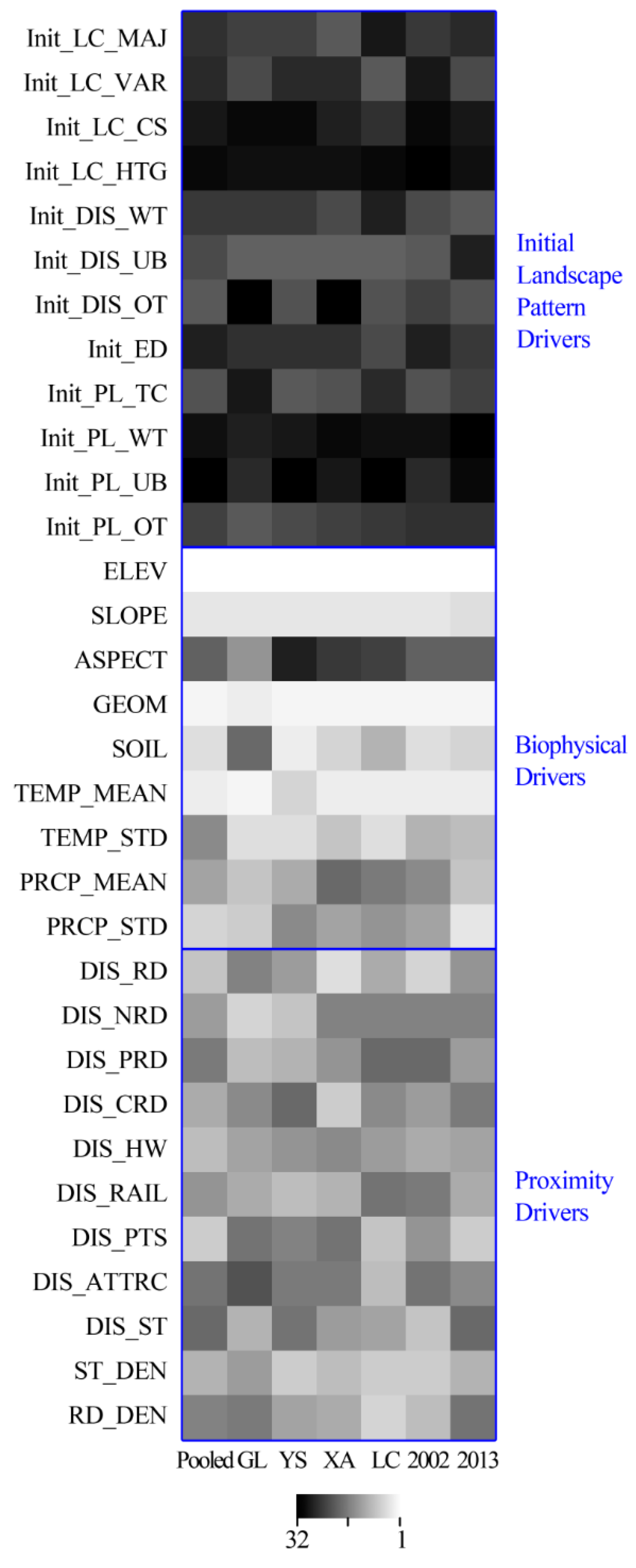
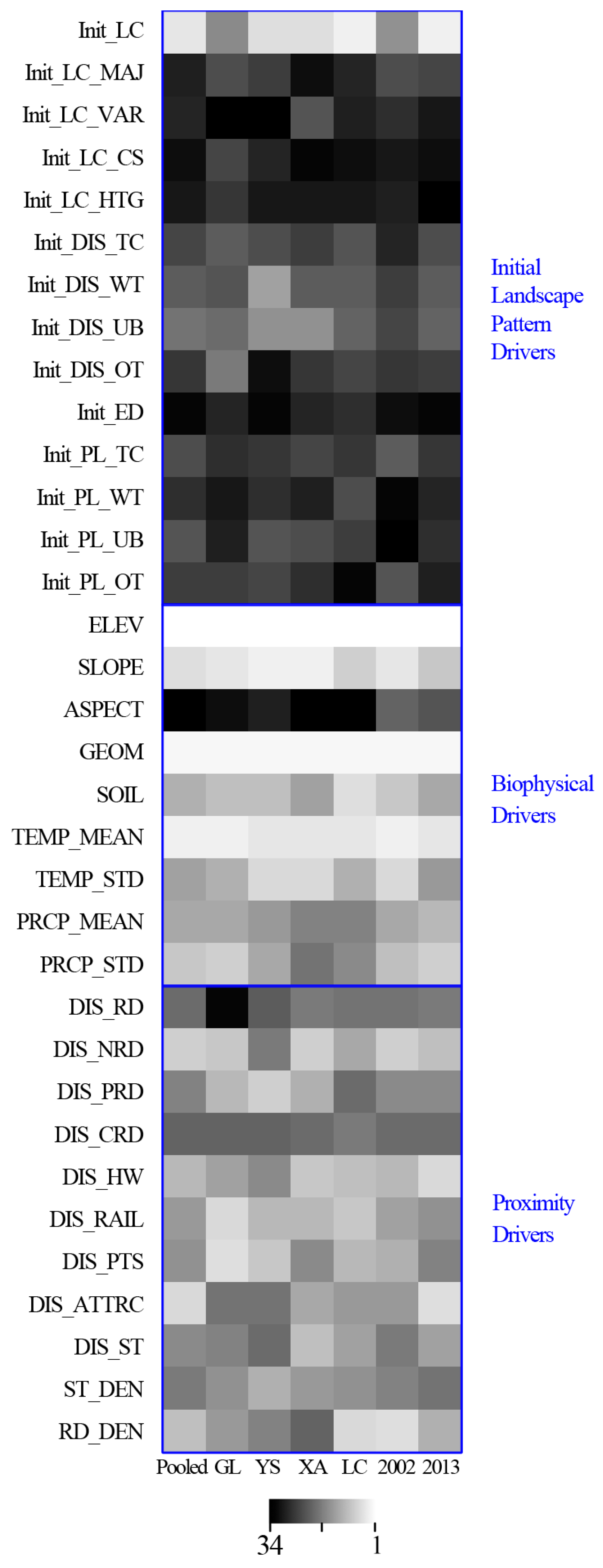
Figure 2 and
Figure 3 using grayscale values, with the brighter squares representing higher ranks. The results of the pooled models can serve as a baseline. However, the interpretation of the pooled models should be done with caution, because it can be biased and misleading without considering the spatio-temporally-variant influence of different factors on tree cover loss and gain probabilities.
3.1. Factors of Tree Cover Loss
The OOB errors of the tree cover loss models for different counties and periods vary within a limited range between 21.98% and 22.47% (
Table 2). Biophysical factors are the most important, and initial landscape pattern factors are the least (
Table S3 and
Figure 2). Seven factors are regarded as important for all six models, demonstrating their general importance. Six of them are biophysical factors, including topographic, soil and temperature factors; the other one is density of settlements, a proximity factor. Six other factors are considered not important and useless in improving the prediction power of all models, including land cover variety (Init_LC_VAR), land cover consistency (Init_LC_CS), land cover heterogeneity (Init_LC_HTG), edge density (Init_ED), the percentage of landscape occupied by water patches (Init_PL_WT) and the percentage of the landscape occupied by urban patches (Init_PL_UB), all of which are initial landscape pattern factors.
The six models identify some common features. Biophysical factors that are closely associated with elevation, including topographic factors and mean annual temperature, exhibit much higher importance than the remaining biophysical factors, evidencing the significance of elevation. Aspect in general has the least importance among all biophysical factors. The temperature factors are generally more important than the precipitation factors, which is consistent with the findings of Aide
et al. and Armenteras
et al. [
2,
56]. The annual mean value is generally more important than the seasonal variation for temperature, while it is the opposite for precipitation. Soil is regarded as very important, because rich soil is more likely to experience tree cover loss by converting to cropland [
24,
57]. The relative importance of proximity factors varies among regions and periods. This implies that though not as important as biophysical factors, proximity factors are significant in explaining the intra-region and intra-period difference of tree cover loss mechanisms. The factors of distances to roads are generally important for all counties and periods, because the cost of access to forests can be greatly reduced by the road network [
58]. The importance of initial landscape pattern factors is low. The factors of immediate neighbors are less important than those of the 200-m radius neighborhood.
A comparison among county models reveals the spatially-variant variable importance. Soil is much less important in Guilin than in Yangshuo, because soils have less variety in Guilin. Precipitation factors are more important in more humid Guilin by ranking seventh and eighth, while the ranks are greater than 10 in other counties. This finding is consistent with Hoyos
et al., who concluded that precipitation may be significant in influencing the tree cover loss caused by agricultural expansion, and the tree cover loss is much more pronounced in more humid regions [
59]. Many studies have recognized the importance of distance to roads as a factor influencing tree cover loss [
60]. However, few have discriminated road types and evaluated the influence of distances to different types of roads [
61,
62]. Different road types indicate different paving, width and traffic flow and can further represent different levels of accessibility and human activity intensity [
63]. This is expected to cause the relative importance of distances to different types of roads to vary across counties. For example, the higher-level roads are more important in Guilin and Yangshuo, while it is opposite in Xing’an. Distance to urban patches was the most important among factors of distances to different types of patches. The percentage of tree cover was more important than the rest of the three PLAND factors in Yangshuo and Xing’an, and the percentage of other land cover was more important in Guilin and Lingchuan.
The number of important factors for tree cover loss in the period of 2002 to 2013 is much smaller, and the OOB error is higher, as compared to the period of 1991 to 2002. Almost all factors that are important within the later period are also important within the earlier period. Generally, the importance of biophysical factors increased while that of proximity and initial landscape pattern factors decreased. Specifically, the importance of climatic factors increased, while that of the other biophysical factors in the two periods is comparable. The importance of density variables decreased. The distances to all types of roads were considered important in 1991 to 2002, while only distance to the highway was important in 2002 to 2013. Initial landscape pattern factors are only included in the model for the earlier period, indicating their decreased importance.
3.2. Marginal Effects of Important Factors on Tree Cover Loss
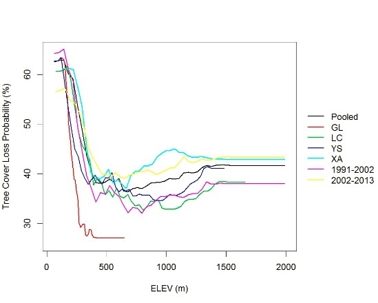
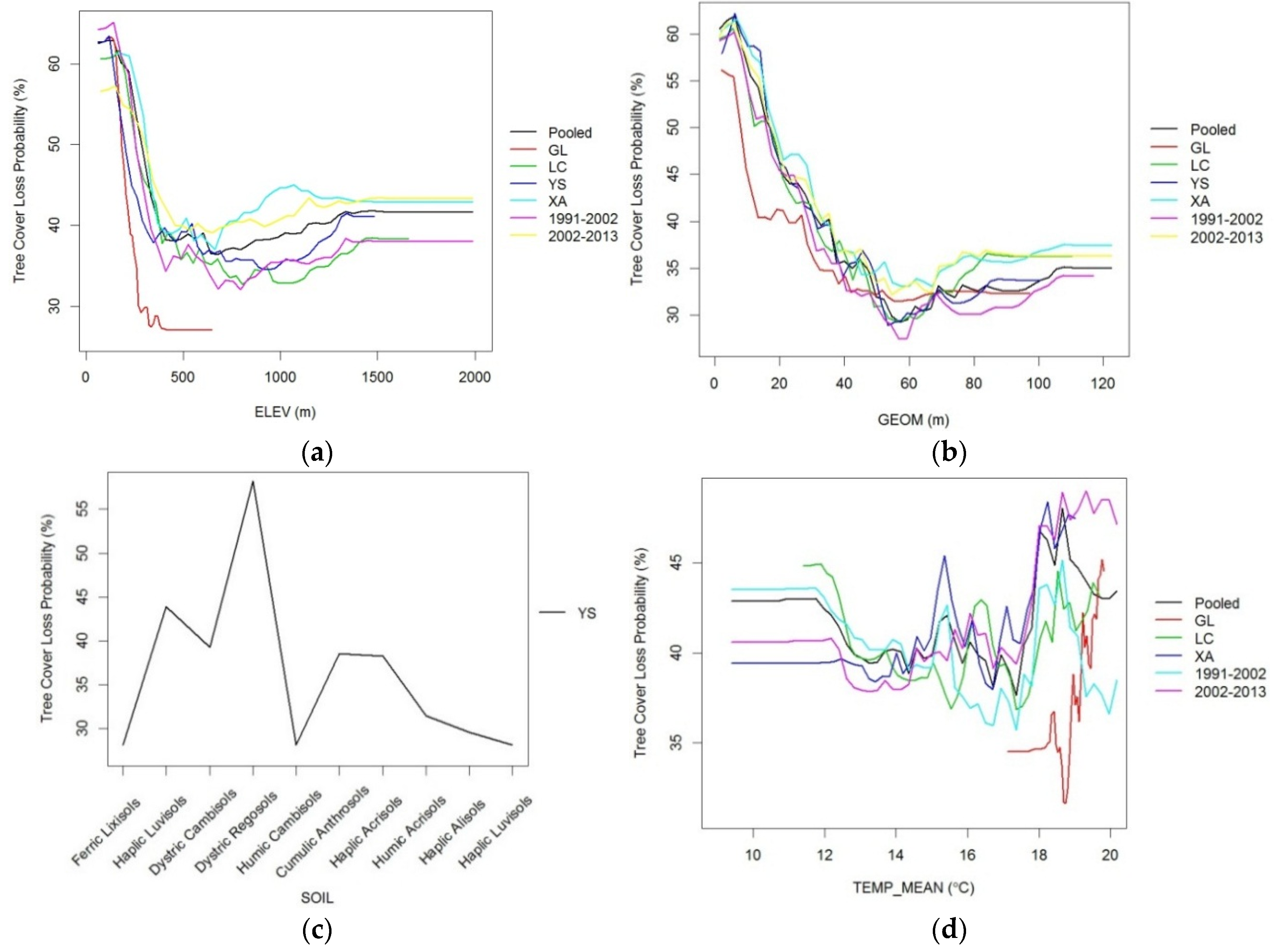
Elevation, geomorphological complexity and annual mean temperature are the three most important factors for all models, except for the model in YS, where soil replaced mean annual temperature as the third most important factor. The partial dependence plots illustrated the marginal effects of the four factors on tree cover loss probability (
Figure 4). Each factor’s influence on tree cover loss probability shared similar trends in different counties and periods.
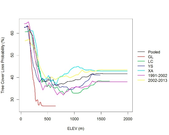
Elevation undoubtedly ranks as the most important factor for all six models. The tree cover loss probability decreases rapidly as elevation increases up until 250 to 500 m dependent on the county or period. Beyond this elevation threshold, the decrease becomes much slower and is followed by an increasing trend in all counties and periods, except for in Guilin. Guilin has the lowest tree cover loss probability beyond 200 m, indicating that a pixel at the same elevation is least likely to experience tree cover loss in Guilin among the four counties. The mountainous Xing’an generally has the highest tree cover loss probability at all elevations. The high tree cover loss probability at higher elevations around 1000 m in Xing’an is probably caused by infrastructure encroachment into mountainous areas. The tree cover loss probabilities of Lingchuan and Yangshuo are in between. Generally, the probability was higher in Lingchuan when elevation is less than 400 m and higher in Yangshuo beyond 400 m. The partial dependence curves of elevation for the two periods reveals that tree cover loss became more likely to occur at higher elevations above 250 m and less likely on lower ones. This is to be expected. With intense human activities and rapid economic development, the remaining tree cover at lower elevations are mostly for recreational purposes and, therefore, less likely to experience tree cover loss.
The tree cover loss probability also decreases when geomorphological complexity increases, though not as rapidly as when elevation increases. The tree cover loss probability tends to be stable beyond a certain threshold. Guilin has the lowest tree cover loss probability when GEOM is less than 40 meters and evolves to have higher probability than Lingchuan and Yangshuo when GEOM values are between 50 and 70 m. Xing’an has the highest probability almost at all values of GEOM. The tree cover loss probability becomes higher at the same level of geomorphological complexity in 2002 to 2013 than in 1991 to 2002. Both partial dependence plots of elevation and geomorphological complexity reveal that the protection of topography on tree cover attenuated when the level of development is high.
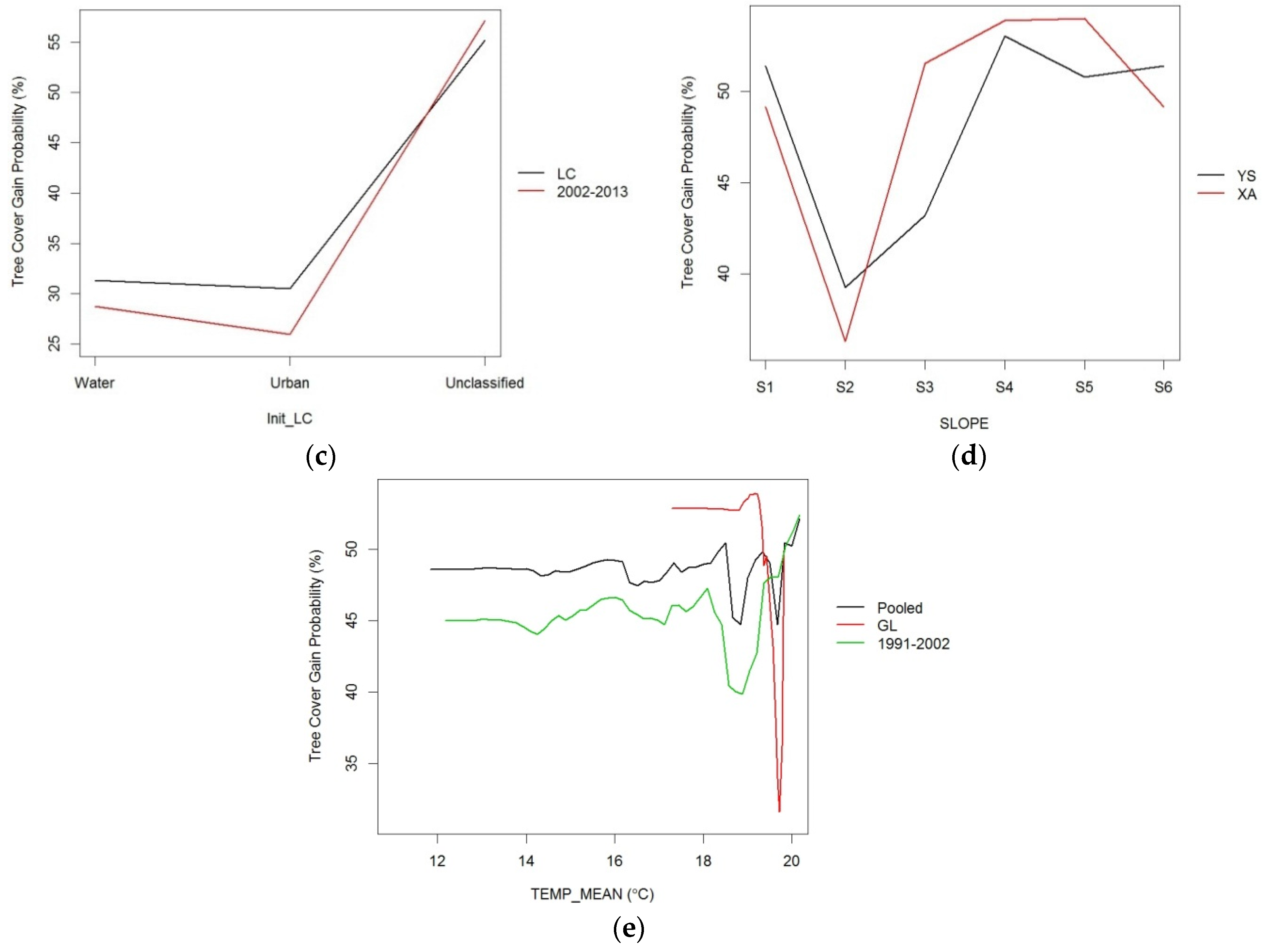
Soil is only ranked top three in Yangshuo.
Figure 4c shows how soil types influence the tree cover loss probability. The x axis shows the soil type according to the FAO-90 soil classification system. Dystric Regosols, a soil type that can be commonly observed for eroding lands, were shown to have the highest tree cover loss probability. Ferric Lixisols, Humic Cambisols and Haplic Luvisols have the lowest tree cover loss probabilities.
The dependence between mean annual temperature and tree cover loss probability is complicated. This is because the mean annual temperature and tree cover loss interrelate. Tree cover loss is more likely to occur in regions with lower mean annual temperatures. Firstly, the mean annual temperature is closely associated with elevation. The lower altitude locations have higher mean annual temperatures, and the high accessibility of these locations necessarily led to a higher tree cover loss probability. Another situation is that regions close to urban or barren areas also tended to have high annual mean temperature because of the decreased evapotranspiration in the neighborhood. This determines that these regions have a higher accessibility and disturbance level, leading to an increased tree cover loss probability.
3.3. Factors of Tree Cover Gain
The OOB errors of the tree cover gain models are higher than those of the tree cover loss ones, ranging from 27.93% to 28.35% (
Table 3). This suggests that tree cover gain probability is more difficult to explain using the potential factors proposed in this paper. This difficulty is probably because that tree cover gain requires more human intervention, whose effect is more difficult to assess quantitatively. There are 16 out of 34 factors that are important for all counties and periods. These 16 factors include most biophysical factors, a majority of proximity factors and two initial landscape pattern factors.
Elevation is the most important factor for both tree cover loss and gain in the LRB, regardless of counties and periods. Slope, geomorphological complexity and mean annual temperature, which are closely related to elevation, are the most important biophysical factors. Aspect is the least important. Temperature factors are more important than precipitation factors. These features for tree cover gain are consistent with those for tree cover loss. As represented by the greyscale values, Distance to national roads, highways, railways and public transportation stations are generally the most important proximity factors. The spatio-temporal variations of proximity factors for tree cover gain were smaller than those for tree cover loss, and therefore, more common features can be observed: distances to higher-level roads are generally more important; distance to all roads is not as important as distances to different types of roads; in most models, except for the Xing’an model, road density is more important than distance to roads. Initial land cover is much more important than the initial landscape pattern of the neighborhood in determining tree cover gain probability, as indicated by the much brighter strip of the first row in
Figure 3. Distances to four land cover types are also very important initial landscape pattern factors. Distances to water and urban patches are generally more important than distances to the other two types of patches. As stated in
Section 3.1, distance to urban patches is also an important initial landscape pattern factor for tree cover loss. Its overall importance as quantified by the importance rank is higher for tree cover gain than tree cover loss. This may indicate that while human activity is important for both tree cover loss and gain, tree cover gain requires more human intervention.
Tree cover gain models for counties reveal that each county has unique features in terms of factors influencing tree cover gain probability. The importance rankings of biophysical factors are highly concordant among counties with only limited variations. Precipitation factors were more important in Guilin than in other counties for both tree cover loss and gain. It may also be hypothesized that precipitation factors are more important for tree cover gain in more humid areas. On the other hand, while annual mean temperature is quite important for all counties, Standard deviation of monthly temperature (TEMP_STD) is more important in Yangshuo and Xing’an than in other counties. Yangshuo is characterized by high average and low seasonal variation of temperature, while Xing’an by low average and high seasonal variation. Lingchuan and Guilin have intermediate values of the average and seasonal variation. It is interesting that TEMP_STD is more important in counties with either high mean temperature or high seasonal variation of temperature. Each county shows more uniqueness in terms of the importance of proximity factors. Though generally higher-level roads are deemed more important, distance to provincial roads is more important than distances to other types of roads in Yangshuo. In attraction-intensive Guilin and Yangshuo, distance to attractions is less important than in the other two counties. This is probably because the spatial variability of distance to attractions in Guilin and Yangshuo is limited and, therefore, is less effective in identifying locations of tree cover gain. As for the initial landscape pattern factors, though initial land cover is the most important of this category, it is much less important in Guilin. This indicates that the tree cover gain in Guilin took place more independently of the initial land cover. While distance to urban patches is of universal importance, distance to water patches is even more important in Yangshuo and distance to other land cover more important in Guilin.
The tree cover gain models for different periods suggest that locations of tree cover gain in the earlier period are easier to map: a smaller set of important factors led to a lower OOB error. The important factors for tree cover gain for 1991 to 2002 are a subset of those for 2002 to 2013. These indicate that there are more uncertainties associated with the tree cover gain within the period of 2002 through 2013. This is probably because of the improved environmental awareness reflected in the national policies, regional programs and civilian initiatives [
13,
64]. The public participation of environmental protection, as compared to national forest programs and natural regeneration, considers less the suitability for forest growth and, therefore, makes the tree cover gain in the latter period more difficult to model. Distance to highways is more important in the latter period. As most highways were actually built in the late 2010s, the increased importance of distance to highways is to be expected. Since the newly-built highways diverted traffic volume, it is reasonable for the ranks of distances to other types of roads, to railways and to public transportation stations to remain the same or become lower. With regard to the initial landscape pattern factors, the rank of initial land cover changed from 15 to three, indicating that it has much more importance in the latter period.
3.4. Marginal Effects of Important Factors on Tree Cover Gain
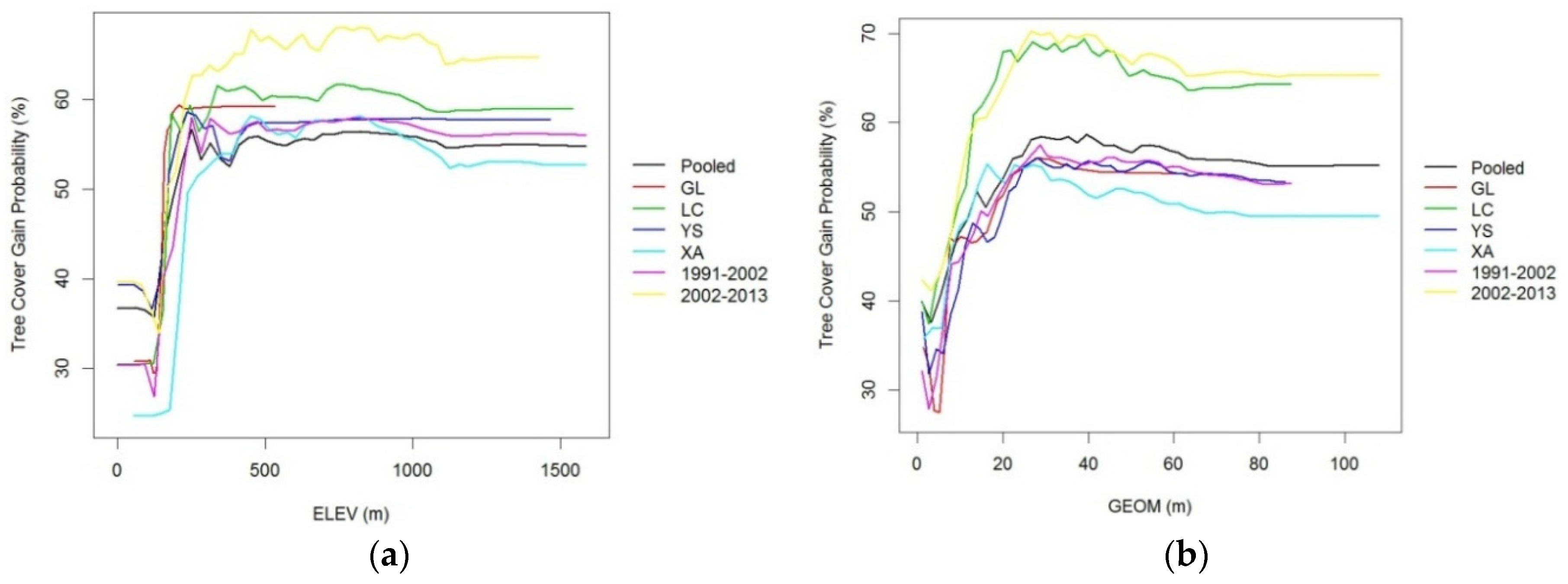
There are five factors that are considered most important, including elevation, geomorphological complexity, initial land cover type, slope and mean annual temperature. Elevation ranks first for all regions and periods. The influence of elevation on the tree cover gain probability in different counties and periods shares a similar trend (
Figure 5a): tree cover gain probability increases dramatically and stabilizes beyond a certain threshold. This trend is an inverse of tree cover loss probability as influenced by elevation. Generally, at the same elevation, the tree cover gain probability is the highest in Lingchuan and the lowest in Xing’an. The tree cover gain probability increases dramatically from the period of 1991 to 2002 to the period of 2002 to 2013. Geomorphological complexity ranks second for all six models. Its influence is very similar to that of elevation, yet the increase rate is not as abrupt and rapid. At the same level of geomorphological complexity, the tree cover gain probability is much higher in Lingchuan than in other counties. The tree cover gain probability also increased from 1991 to 2002 to 2002 to 2013 at all levels of geomorphological complexity.
Initial land cover is among the top three most important factors in Lingchuan and in the period of 2002 to 2013. As shown in
Figure 5c, both partial dependence curves indicate that the other land cover patches are much more likely to experience tree cover gain than water and urban patches. Other land cover patches mainly include barren lands, grassland and cropland, and it is obviously easier for them to be converted to tree cover. This is largely associated with the implementation of the nationwide Sloping Land Conversion Program (SLCP) in 2002, which promotes the conversion of sloping cropland to tree cover [
13]. Slope ranks the third in Yangshuo and Xing’an. Generally, steeper slopes promote tree cover gain. As with tree cover loss probability, the annual mean temperature’s influence on tree cover gain probability is also complicated, but generally, the curves include a stable stretch, a decreasing part and an increasing part as temperature increases.
4. Conclusions
This paper aims to identify the factors that influence the locations of tree cover loss and gain at the pixel level and to evaluate the importance of these factors in the four counties and two periods in the LRB. Three categories of factors were considered, including initial landscape pattern factors, biophysical factors and proximity factors. The random forests modeling technique was used to model the responses of tree cover loss and gain probabilities of sampled pixels to three categories of factors. The metric of the mean decrease in accuracy was used to quantitatively evaluate the importance of factors in different regions and periods. The relative importance of factors was compared among regions and periods to reveal the spatio-temporal heterogeneity. A set of important factors was derived for each region and period according to the smallest mean OOB error. The partial dependence plots were generated for the three most important factors for each region and period, in order to reveal the exact variation of tree cover loss and gain probabilities as influenced by different factors.
The modeling results indicate that biophysical factors are the most important, and initial landscape pattern factors are the least for both tree cover loss and gain. The importance of factors for tree cover loss and gain is heterogeneous across space and time. The tree cover gain models are associated with higher OOB errors as compared to the tree cover loss models. This indicates that where tree cover gain occurs, it is more difficult to explain using the potential factors and may be attributed to more human intervention required by tree cover gain.
Elevation is the most important in determining the locations of tree cover loss and gain in the LRB, irrespective of counties and periods. Moreover, the factors that are closely associated with elevation, including slope, geomorphological complexity and annual mean temperature, are also among the most important factors. The areas with high elevation and complex topography are associated with low accessibility and disturbance levels, providing protection to the tree cover and leading to high tree cover gain and low tree cover loss probabilities. Topography’s protection attenuated when the development level is high. Temperature factors are generally more important than precipitation factors, while precipitation factors may be more important in humid regions for both tree cover loss and gain. The importance rankings of biophysical factors are highly consistent across time and region, while each county and period exhibits more uniqueness in terms of the importance of proximity factors and initial landscape pattern factors. The spatio-temporal variations of importance of proximity factors for tree cover gain are smaller than those for tree cover loss. Therefore, while common features are difficult to be extracted from different tree cover loss models, some common features can be identified for tree cover gain models. An outstanding one is that distances to higher-level roads are generally more important for tree cover gain. Though initial landscape pattern factors are of much less importance for both tree cover loss and gain, the initial land cover is considered to be very important for tree cover gain. The initial landscape pattern of immediate neighbors is less important than those of the 200-m radius neighborhood.
The model performance can be potentially improved if the following issues are satisfactorily addressed. As stated in
Section 2.2, croplands are difficult to distinguish from degraded rangeland and barren land, because most scenes were acquired in the dry season. However, adopting a land cover classification system including cropland is beneficial, because the SLCP has greatly promoted reforestation by encouraging the conversion of sloping cropland to forest [
13]. Identifying cropland thereby can better explain the tree cover gain in the study area.
Nature reserves have been continuously established in the study area following the implementation of the Nature Reserve Construction Program (NRCP). Incorporating the nature reserve as one of the factors is expected to improve the model performance upon the acquisition of reliable boundaries of nature reserves. It is also worthwhile to explore the variant factors of tree cover loss and gain in nature reserves and other areas and to analyze the influence of the nature reserve on the probabilities of tree cover loss and gain.
Different regions and periods are characterized by distinct combinations of factor values. For example, Guilin is characterized by low values of distance to roads, low elevation and low levels of geographical complexity. Therefore, the performance of tree cover loss and gain models is expected to increase if separate models are built directly for different intervals of factors, instead of for different regions and periods. This can be achieved by applying a multivariate clustering on the sampled cases and using the cases in each cluster to build separate models. However, this approach makes it more difficult to associate factors with specific administrative regions and time periods, thereby limiting its practical applications.
This paper identified potential factors influencing the locations of both tree cover loss and gain at the pixel level, with the seldom considered initial landscape pattern factors taken into account. It also demonstrated an approach of evaluating the variable importance of factors. The analysis of spatio-temporally-variant variable importance furthers the understanding of how different factors took effect in the counties and periods with different developmental stages, climatic conditions, landscape composition and other characteristics. The findings are expected to assist with the policy-making and administrative planning concerning ecosystem conservation, infrastructure development and land management.


