Spatial Up-Scaling Correction for Leaf Area Index Based on the Fractal Theory

Abstract

The scaling effect correction of retrieved parameters is an essential and difficult issue in analysis and application of remote sensing information. Based on fractal theory, this paper developed a scaling transfer model to correct the scaling effect of the leaf area index (LAI) estimated from coarse spatial resolution image. As the key parameter of the proposed model, the information fractal dimension (D) of the up-scaling pixel was calculated by establishing the double logarithmic linear relationship between D-2 and the normalized difference vegetation index (NDVI) standard deviation (σ_NDVI) of the up-scaling pixel. Based on the calculated D and the fractal relationship between the exact LAI and the approximated LAI estimated from the coarse resolution pixel, a LAI scaling transfer model was established. Finally, the model accuracy in correcting the scaling effect was discussed. Results indicated that the D increases with increasing σ_NDVI, and the D-2 was highly linearly correlated with σ_NDVI on the double logarithmic coordinate axis. The scaling transfer model corrected the scaling effect of LAI with a maximum value of root-mean-square error (RMSE) of 0.011. The maximum absolute correction error (ACE) and relative correction error (RCE) were only 0.108% and 8.56%, respectively. The spatial heterogeneity was the primary cause resulting in the scaling effect and the key influencing factor of correction effect. The results indicated that the developed method based on fractal theory could effectively correct the scaling effect of LAI estimated from the heterogeneous pixels.

1. Introduction

Spatial scaling correction is an essential and difficult issue in analysis and application of remote sensing information. Scale effect are highly correlated with many issues, such as parameters inversion [1,2], objects classification [3,4], agricultural and ecological data assimilation [5,6], remote sensing product validation [7,8], and data fusion [9]. Therefore, it is necessary to comprehensively explore the scaling effect correction. Leaf area index (LAI) is an important land surface parameter in running both land surface and global atmospheric circulation models [10,11,12,13]. The scaling effect of LAI estimated from remote sensing data is deeply studied in the aspect of phenomenon description, cause analysis, and establishment of the scale transformation relationships. Previous studies have shown that the spatial resolutions correlated nonlinearly with the LAIs estimated at different spatial resolutions [14,15]. Compared with the nonlinearity of the LAI retrieval models or algorithms, the spatial heterogeneity is the main factor resulting in the phenomenon [16,17,18]. In order to quantitatively describe and reduce (or eliminate) the scaling effect, some empirically linear or nonlinear transformation relationships among LAIs at different resolutions have been established with statistical methods [19,20,21,22,23]. However, since these empirical models were established using a large amount of sample data and lacked a clear theoretical interpretation, several general models were proposed based on mathematical theory or the biophysical mechanism of scaling effect [24,25,26,27,28]. For instances, Hu and Islam suggested a method by establishing the relationship between variance, covariance and the mean values of parameters at the pixel scale [24]. On the basis of this method proposed by Hu and Islam, Garrigues et al. extended the Taylor expansion to correct the scaling effect using a multivariate transfer function [25]. A spatialization model named computational geometry method (CGM) was developed by Raffy to reduce the scaling effect [26].

During the commonly used methods for scale transformation, fractal theory performs well in describing how the study objects evolved with scale changing [29,30,31]. The essence of fractal theory is scale transformation. Fractal theory is used to describe and study an object with the following characteristics: (1) the part and the whole of the object are similar (self-similarity); and (2) the characteristic length of the object does not exist, namely it is scale-free. Li et al. pointed out that fractal (or similar fractal) relationship is one of the three different transformation tendencies that are used for describing scaling effect [32]. As a classic scale transformation method, fractal could quantitatively describe the transformation law of the object on a continuous scale [30,31]. In addition, the fractal method is more general compared with the empirical method. Compared with the biophysical model, the fractal method has the potential, namely introducing less parameters to provide a more concise and clear description about the spatial-temporal variation of the object, and thereby it generates a more practical model for scale transformation [33,34]. Several studies for scaling effect correction based on fractal theory have been carried out. Liu [35] and Jiang et al. [36] found that the high frequency coefficients, acquired by Haar wavelet decomposition, of LAIs retrieved at finer spatial resolution and the scaling bias of neighboring scales obey a fractal relationship. However, the proposed fractal relationship could only be suitable for neighboring scales, possibly due to the dyadic property of the Haar wavelet. Zhang et al. defined the information fractal of remote sensing products and applied it to describe the scale transformation law of the LAIs estimated from different resolution images [7]. Although the information fractal is an efficient tool for the description of scaling effect, the proposed method based on information fractal in reference [7] was neither suitable for LAI calculation at different resolutions nor for scaling effect correction. Through extending the method of Zhang et al. [7], the authors established an image-based LAI scaling transfer model by using the information fractal dimension (D) [37]. The LAI scaling transfer model was developed by establishing the double logarithmic linear relationship between the scale (spatial resolution) and average LAIs of the image at different scales. However, this model could only calculate the average LAIs of the entire image at different spatial resolutions and evaluate the scaling effect of them. In practical applications, we aim to correct the LAI scaling effect of the coarse resolution image pixel by pixel.

The objective of this paper is to correct the scaling bias (errors due to scaling) of the LAI retrieved from the coarse resolution pixels based on fractal theory, through comparing the images with different resolutions (fine and coarse resolutions). This proposed method in this paper could efficiently realize the scaling effect correction of the estimated LAI at different spatial resolutions with high accuracy. Inspired by the image-based model in reference [37], a pixel-based LAI spatial scaling transfer model using the information fractal dimension D was developed in the current study. In this method, each up-scaling pixel was considered an “image” for using the image-based model to correct the LAI scaling effect of the up-scaling pixel. The key of the idea was the D (the coefficient of the pixel-based model) calculation of each up-scaling pixel. The D of the up-scaling pixel was calculated by establishing the double logarithmic linear relationship between D-2 and the normalized difference vegetation index (NDVI) standard deviation (σ_NDVI) of the up-scaling pixels. Therefore, based on the calculated D and the fractal relationship between the exact LAI (corresponding to the LAI estimated from the fine spatial resolution pixels) and the approximated LAI (corresponding to the LAI derived from the coarse resolution pixels), this new model established the transformation relationship between the exact LAI and the approximated LAI of the up-scaling pixel, and hence it could be used to correct the scaling effect of the LAI estimated from the heterogeneous pixels in the coarse resolution image.

This paper is organized as follows. Section 2 briefly introduces the remote sensing image and ground datasets, and provides a detailed description of the proposed pixel-based LAI spatial scaling transfer model. In Section 3, experimental results of scaling effect correction and the validation using MODIS data are provided to demonstrate the applicability of the new method. Section 4 further discusses the proposed method, followed by conclusions in Section 5.

2. Materials and Methods

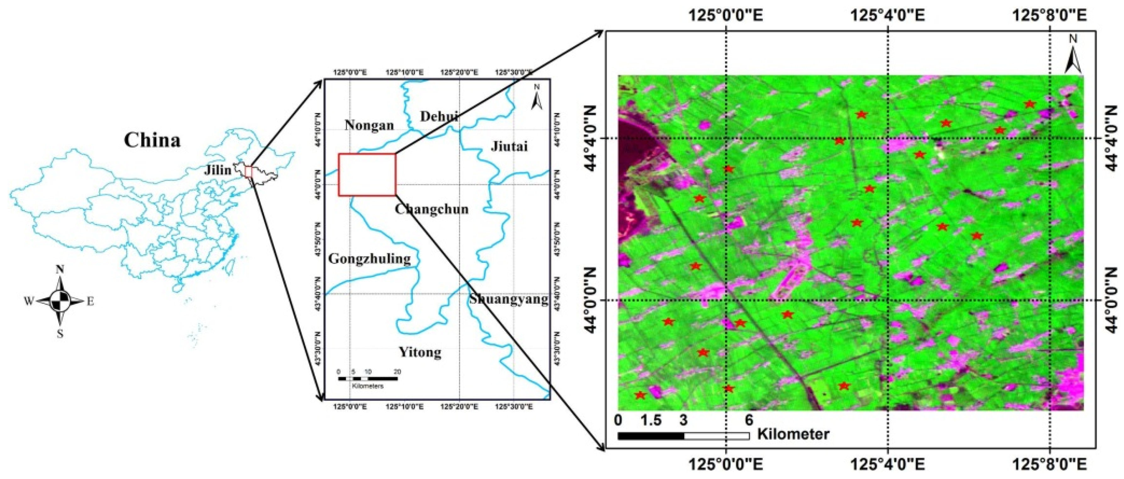
2.1. Materials

The study area (44°01.42′N, 125°03.06′E) is located in a suburb of Changchun City, Jilin Province, China, with a flat terrain. Farmland is the main land-cover class with scattered water bodies, roads, and buildings (Figure 1). Single precocity rice is the dominant crop of the farmlands in this area. In this study, remotely sensed data with a size of 512 × 512 pixels, namely, HJ-1 charge-coupled device (CCD) image, were acquired from the Environment and Disaster Reduction Small Satellites on 29 July 2009, which were successfully launched on 6 September 2008 for monitoring the environment and natural disasters. The CCD cameras in the HJ-1 satellite can capture CCD images with a ground swath width of 700 km and a revisit cycle of 2 days. The CCD image possesses a ground-projected instantaneous field of view (GIFOV) of 30 m and is acquired in four spectral wavebands that mirror those of the IKONOS satellite sensor. These wavebands range from 0.45 μm to 0.52 μm (blue waveband), 0.52 μm to 0.60 μm (green waveband), 0.63 μm to 0.69 μm (red waveband), and 0.76 μm to 0.9 μm (near-infrared waveband). The radiometric calibration, atmospheric correction and geometric rectification for the CCD image were carried out before data application. The radiometric calibration for the CCD image was achieved using the calibration coefficient of each band provided by the China Centre for Resources Satellite Data and Application. Then, the geometric rectification of the CCD image using a rectified TM image was also conducted and the geolocation error of the CCD image was less than one pixel. Finally, the 6S atmospheric radiative transfer model was used for the atmospheric correction. The MODIS image (spatial resolution: 250 m) of the same area was adopted to estimate the MODIS LAI for the validation of the proposed LAI scaling transfer model.

As an efficient indicator of vegetation abundance, the NDVI was adopted for LAI estimation in this study [38]. Twenty sampling sites were selected in the study area (see the red stars in Figure 1). The LAI values of each site (30 m × 30 m) were measured at five points by using LAI-2000 on 30 July 2009, and the average measurements was used to represent the LAI value in each site. The starting point was randomly selected and then the next four points were determined randomly with a distance of 5 m along to the former point. Thereafter, an empirical regression function f (Equation (1)) (Figure 2a) relating LAI to NDVI with a determination coefficient (R²) of 0.814 was established to generate the LAI map (Figure 2c) from NDVI image (Figure 2b).

$$f:LAI=0.2258e^{3.727NDVI}$$

(1)

In this study, the empirical regression function f was specifically applied to investigate the scaling effect of the LAI estimated from the heterogeneous pixels and hence the LAI estimation accuracy is not the focus. The pixels with high spatial resolution (defined as a pixel size of 30 m in this study) were considered homogeneous in this study. Therefore, the regression function f was assumed to be without any scaling effect at high spatial resolution.

2.2. Methods

According to reference [25], the two up-scaling methods of LAI retrieval are shown in Figure 3. As shown in path 1 of Figure 3, the calculation of the exact LAI value (LAI^exa) of a coarse resolution pixel includes the following steps: (1) calculating the corresponding LAI value (LAI_i) of each original high resolution pixel by applying the empirical regression function f to the vegetation index (VI_i) of the original high resolution pixel; and (2) averaging all the LAI_i results of the original high resolution pixels within the coarse resolution pixel. The calculation of the approximated LAI value (LAI^app) of a coarse resolution pixel includes the opposite steps (path 2 in Figure 3): (1) averaging all the VI_i results (VI_m) of the original high resolution pixels within the coarse resolution pixel; and (2) applying f to VI_m of the coarse resolution pixel. The difference between LAI^exa and LAI^app is defined as scaling bias on account of both the spatial heterogeneity of the coarse resolution pixel and the nonlinearity of the empirical regression function f.

As shown in Figure 3, the LAI values of the same object retrieved by the same empirical regression function change with the change of observation scales (spatial resolutions). This phenomenon is similar to the case that the coastline lengths of England are varied when different scales are used [39], which indicates the remotely sensed products are dependent on the pixel scales and the characteristic length of the remotely sensed products does not exist, namely the scale-free phenomenon [7]. Besides, Penland et al. pointed out that the remote sensing images possess the self-similarity characteristics [40]. Scale-free and self-similarity are the foundation of fractal theory established by Mandelbrot [41]. Therefore, fractal theory could be considered as an effective tool to correct the scaling effect of retrieved parameters.

In accordance with fractal theory, the measurements of the study object perform power function correlation with the scales [42]. Consequently, for the jth coarse pixel of an up-scaling remote sensing image with a coarse resolution of n × 30 m, the LAI value LAIm,j of the jth coarse pixel (Equation (2)) calculated using scale m (m = 1, 2, …, n) is a power function of scale m (Equation (3)), i.e.,

$$LA{I}_{m,j}=\frac{1}{{(\frac{n}{m})}^2}{\displaystyle \sum _{g=1}^{{(\frac{n}{m})}^2}f(\frac{1}{m^2}{\displaystyle \sum _{i=1}^{m^2}NDV{I}_{i,g}})}$$

(2)

$$LA{I}_{m,j}=K\times m^{d_{n,j}}$$

(3)

where j is the number of coarse resolution pixels within the up-scaling image (j = 1, 2, …, (N/n)²), and the size of the remote sensing image with a high spatial resolution is N × N original pixels; g is the number of pixels with a size of m × m original pixels within the jth coarse resolution pixel (g = 1, 2, …, (n/m)²); i is the number of the original pixels within the gth pixel with a size of m × m original pixels (i = 1, 2, …, m²); NDVI_i,g is the ith high spatial resolution NDVI value within the gth pixels with a size of m × m original pixels; and d_n,j, the slope of the linear fitting curve of the scale m versus the LAI value LAI_m,j on the double logarithmic coordinate axis, is the scaling parameter related to the information fractal dimension D of the jth coarse pixel. The D of the up-scaling pixel is given by Equation (4) [41].

$$D=2-d$$

(4)

According to the definition of LAI^exa in Figure 3, LAI_1,j is the same as the exact LAI value ${LAI}_{n,j}^{exa}$ of the jth coarse resolution pixel when scale m equals 1 (Equation (5)), which is calculated by first applying f to all high spatial resolution NDVI values within the jth coarse pixel and then aggregating the results of the corresponding LAI. Meanwhile, LAI_1,j equals K according to Equation (3); therefore, K is the same as ${LAI}_{n,j}^{exa}$. Similarly, according to the definition of LAI^app in Figure 3, LAI_n,j is the same as the approximated LAI value ${LAI}_{n,j}^{app}$ of the jth coarse resolution pixel when scale m equals n (Equation (6)), which is calculated by first averaging all high spatial resolution NDVI values within the jth coarse pixel and then applying f to the average NDVI of the jth coarse resolution pixel. Therefore, the transformation of Equation (3) is as follows (Equation (7)):

$$LA{I}_{1,j}=\frac{1}{{(\frac{n}{1})}^2}{\displaystyle \sum _{g=1}^{{(\frac{n}{1})}^2}f(\frac{1}{1^2}{\displaystyle \sum _{i=1}^{1^2}NDV{I}_{i,g}})}=\frac{1}{n^2}{\displaystyle \sum _{g=1}^{n^2}f(NDV{I}_{i,g}})=LA{I}_{n,j}^{exa}$$

(5)

$$LA{I}_{n,j}=\frac{1}{{(\frac{n}{n})}^2}{\displaystyle \sum _{g=1}^{{(\frac{n}{n})}^2}f(\frac{1}{n^2}{\displaystyle \sum _{i=1}^{n^2}NDV{I}_{i,g}})}=f(\frac{1}{n^2}{\displaystyle \sum _{i=1}^{n^2}NDV{I}_{i,g}})=LA{I}_{n,j}^{app}$$

(6)

$$LA{I}_{n,j}^{app}=LA{I}_{n,j}^{exa}\times n^{2-D_{n,j}}$$

(7)

The key of scaling effect correction using Equation (7) is the acquisition of the D. The geometric significance of D computed by Equation (7) is that it can reflect the heterogeneity characteristic of the LAI spatial distribution. The more homogeneous the land surface is, the smaller the fractal dimension is. Obviously, the D of the up-scaling pixel is 2 when the land cover type is homogeneous. The NDVI standard deviation σ_NDVI of the up-scaling pixel can represent the spatial heterogeneity of the up-scaling mixed pixel, and hence a correlation should exist between D and σ_NDVI. Therefore, the D of each up-scaling pixel can be acquired by establishing the relationship between the D (or transformation form of D) and the σ_NDVI of the up-scaling pixel. Based on the calculated D and the fractal relationship between the exact LAI ${LAI}_{n,j}^{exa}$ and the approximated LAI ${LAI}_{n,j}^{app}$ (Equation (7)), the ${LAI}_{n,j}^{app}$ retrieved from a coarse spatial resolution pixel can be corrected to the corrected LAI ${LAI}_{n,j}^{corr}$ using the proposed LAI scaling transfer model in this study (Equation (8)).

$$LA{I}_{n,j}^{corr}=LA{I}_{n,j}^{app}\times n^{D_{n,j}-2}$$

(8)

3. Results and Analysis

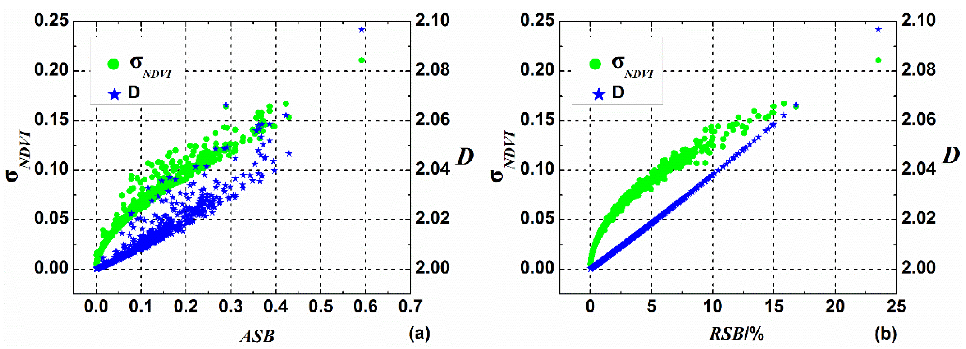
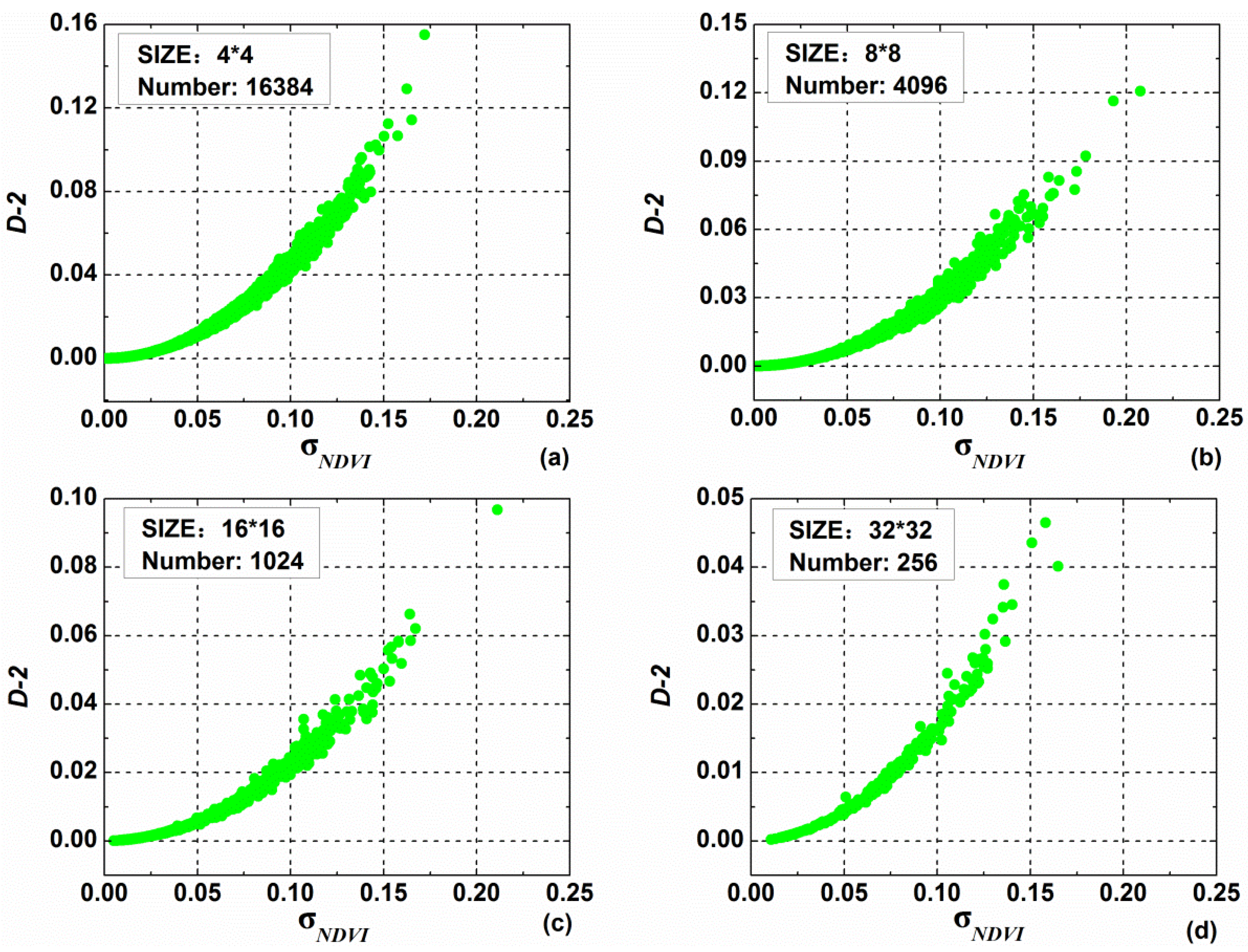
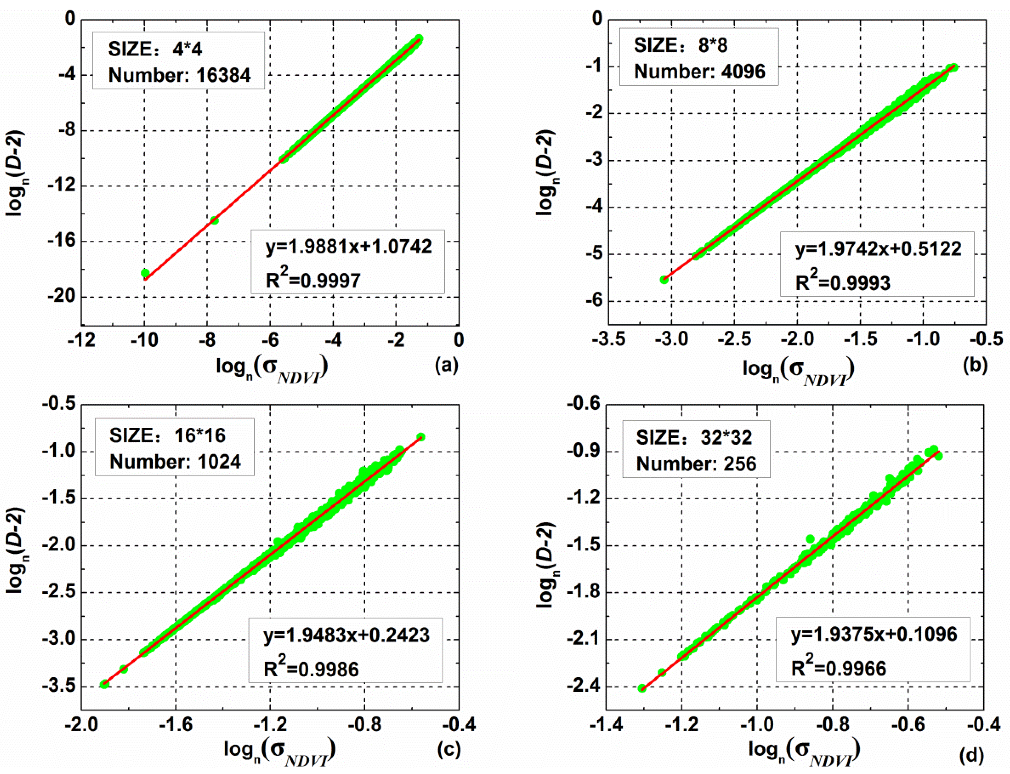
3.1. Calculation of Information Fractal Dimension

As mentioned in Section 2.2, a correlation should exist between D and σ_NDVI. Considering the up-scaling pixels of sizes 4 × 4, 8 × 8, 16 × 16, and 32 × 32 original pixels for example in this study, the CCD image of size 512 × 512 original pixels was divided into 16,384, 4,096, 1024, and 256 up-scaling pixels of sizes 4 × 4, 8 × 8, 16 × 16, and 32 × 32 original pixels, respectively. The relationships between D-2 (-d in Equation (4)) and σ_NDVI of the up-scaling pixels at four different spatial resolutions were established, respectively (Figure 4). From Figure 4, regardless of the size of the up-scaling pixels, the D of the up-scaling pixels increased with increasing σ_NDVI, and D-2 had power law dependence at σ_NDVI. Therefore, a linear empirically determined function (Equation (9)) that is used to estimate D was developed by applying a log transformation on both D-2 and σ_NDVI (Figure 5). The R² were almost equal to 1 at four different spatial resolutions, thereby indicating the high correlation between D-2 and σ_NDVI. Hence, based on the known σ_NDVI of the up-scaling pixels and the linear empirically determined function, the D of the up-scaling pixels could be calculated, which provides the foundation for scaling effect correction using the LAI scaling transfer model (Equation (8)). Although establishing the empirically determined function using all pixels of an image is unrealistic in practical application, the R² of the function were almost equal to 1. Thus, the difference of fitting parameters (a and b in Equation (9)) between the calculation using all pixels and the calculation using part of all pixels was insignificant. Selecting representative sample data within the range of σ_NDVI to establish the function for calculating information fractal dimension D is therefore feasible.

$${\text{log}}_n(D-2)=a\times {\text{log}}_n\left({\sigma }_{NDVI}\right)+b$$

(9)

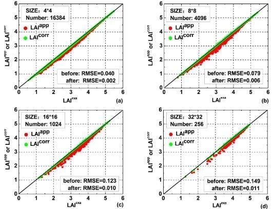
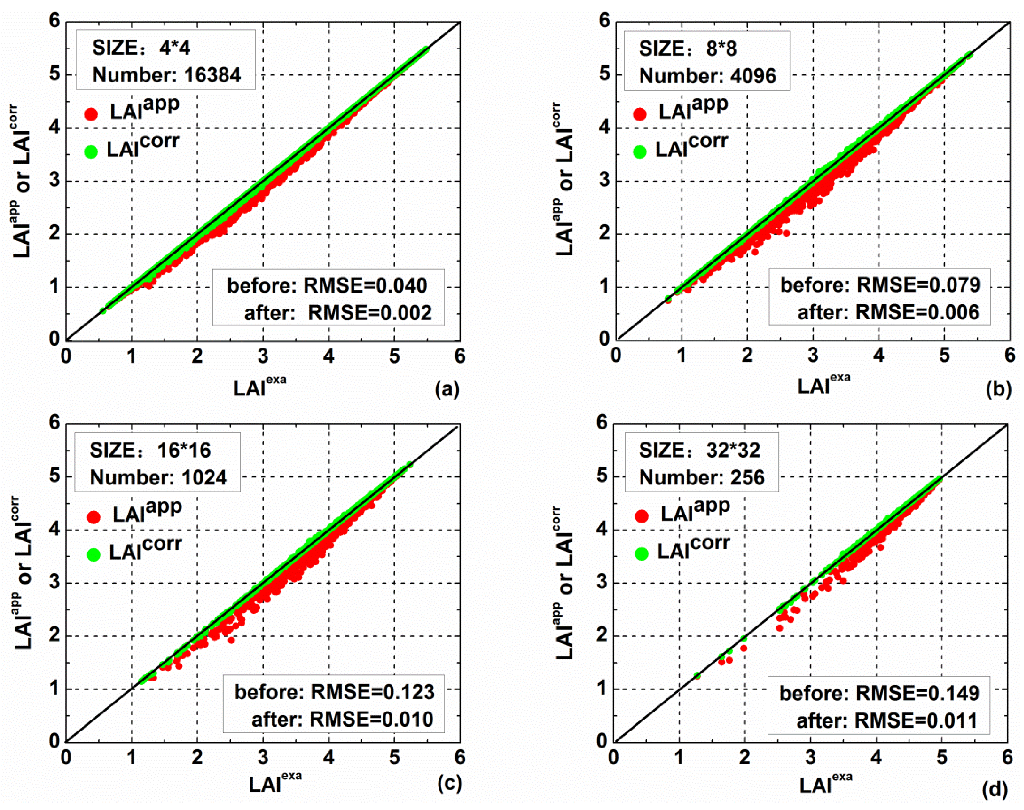
3.2. Correction of Scaling Effect

According to previous studies [18,25], the scaling bias of the LAI derived from the up-scaling pixel is closely correlated with the spatial heterogeneity of the up-scaling mixed pixel. The scatterplots between σ_NDVI (or D) and absolute scaling bias (ASB) (Equation (10)) (or relative scaling bias (RSB) (Equation (11))) were drawn to analyze the influence of spatial heterogeneity on scaling effect (Figure 6). Figure 6 shows that the ASB (or RSB) of LAI inversion increased with an increase in σ_NDVI (or D) of the up-scaling mixed pixel. Strongly, linear dependence of RSB on D was observed. This proved that the spatial heterogeneity of land surface is the primary source of the scaling effect of LAI. From Figure 6, the maximum RSB was almost to the point of 25%, and therefore the scaling effect of LAI caused by the spatial heterogeneity could not be ignored and should be corrected.

By using the D derived from Equation (9), the LAI correction value LAI^corr was computed by the LAI scaling transfer model (Equation (8)). By comparing the LAI^corr, the exact LAI LAI^exa, and the approximated LAI LAI^app (Figure 7), LAI values were distributed in the lower right of the scatterplot before correction, thereby indicating the underestimation of the LAI retrieved from the remote sensing image with a coarse spatial resolution. After correction, the root-mean-square error (RMSE) significantly decreased, with a maximum value of only 0.011 at four different spatial resolutions. The two values of LAI^corr and LAI^exa were close. Accordingly, the developed method for LAI spatial scaling effect correction based on fractal theory is effective.

$$ASB=LA{I}^{exa}-LA{I}^{app}$$

(10)

$$RSB=\frac{LA{I}^{exa}-LA{I}^{app}}{LA{I}^{exa}}$$

(11)

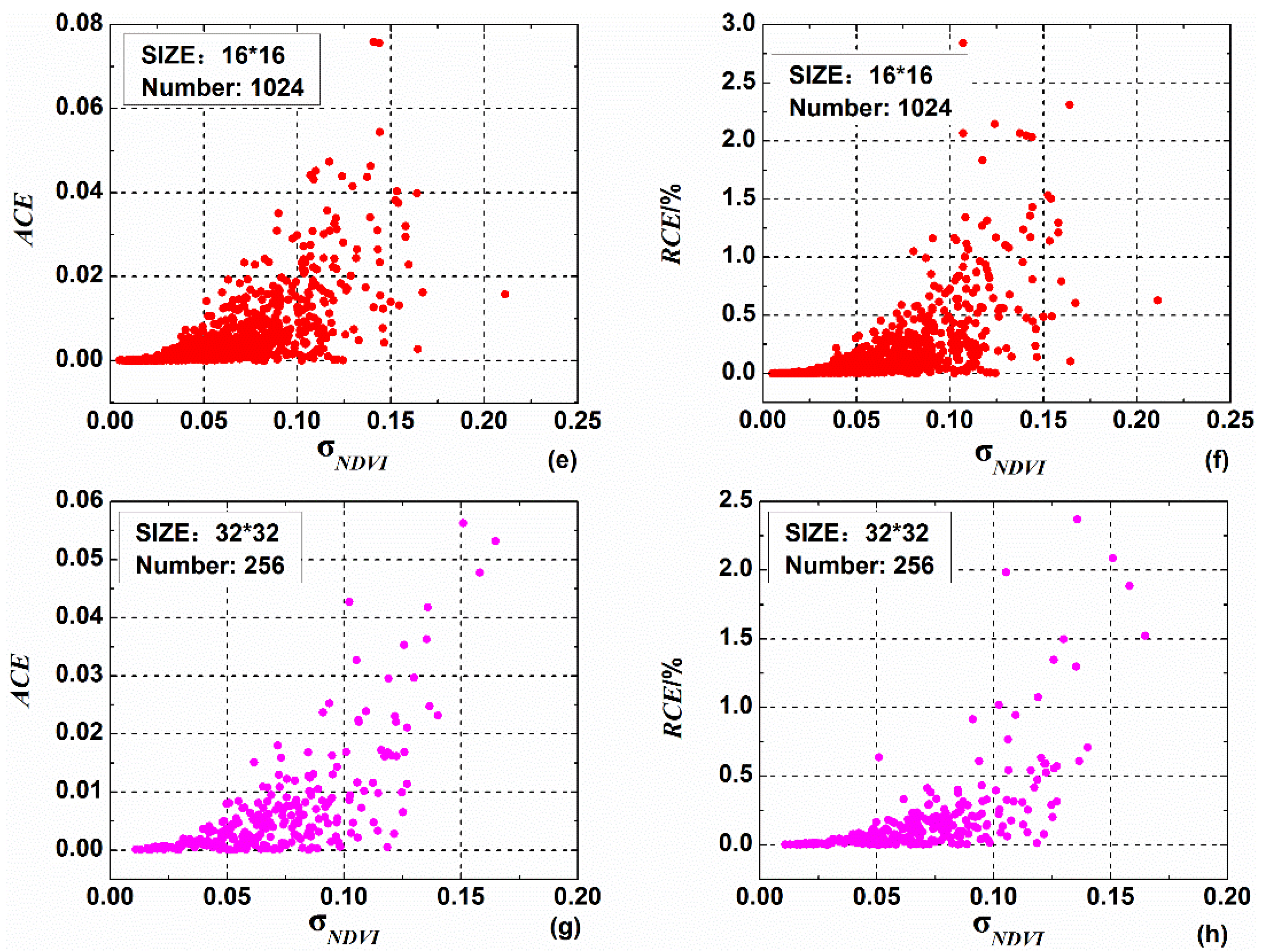
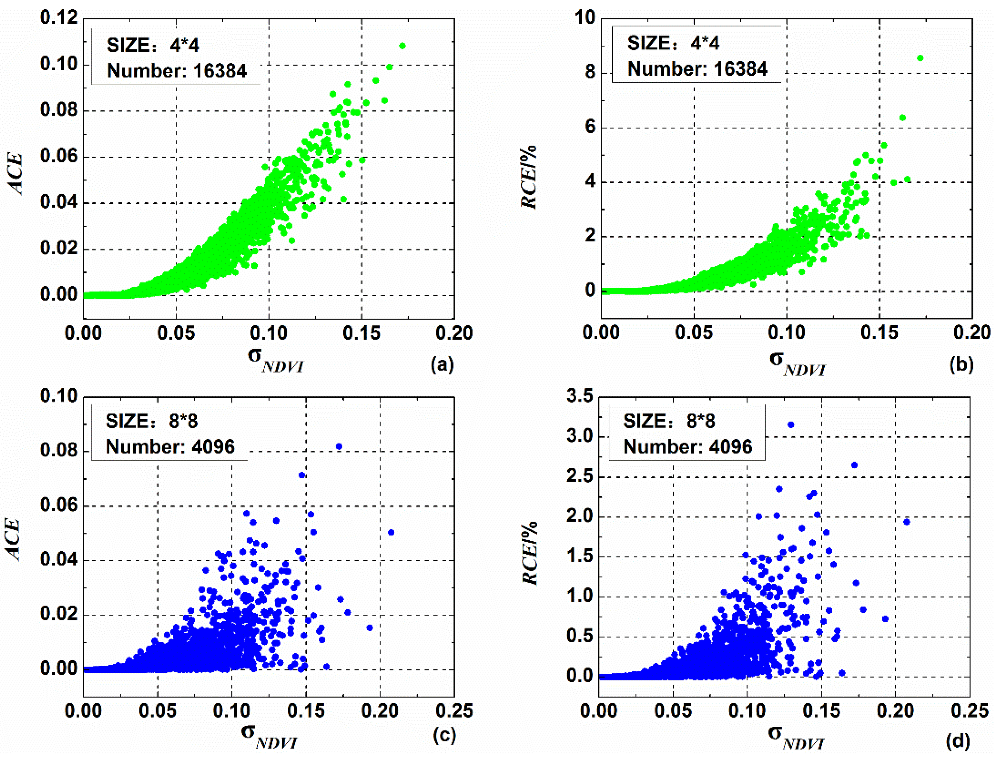
3.3. Analysis of Correction Error

To analyze the correction effect using the proposed method, two indicators of absolute correction error (ACE) (Equation (12)) and relative correction error (RCE) (Equation (13)) were defined, and the scatterplots between two indicators and σ_NDVI were drawn (Figure 8). From Figure 8, the ACE and the RCE generally increased with increasing σ_NDVI, which means that the correction effect is relatively insignificant when σ_NDVI is large. The maximum ACE and RCE corresponded to the low and medium LAI values at four different resolutions (

Table 1. Maximum ASB and RSB before correction and Maximum ACE and RCE after correction.

Scale/Pixels	Before Correction				After Correction
	Maximum ASB	Corresponding LAIexa	Maximum RSB/%	Corresponding LAIexa	Maximum ACE	Corresponding LAIexa	Maximum RCE/%	Corresponding LAIexa
4 × 4	0.353	2.407	19.35	1.265	0.108	1.265	8.56	1.265
8 × 8	0.576	2.595	22.21	2.595	0.082	3.094	3.15	1.098
16 × 16	0.591	2.514	23.52	2.514	0.076	3.709	2.84	1.554
32 × 32	0.454	3.499	14.88	2.533	0.056	2.695	2.37	1.763

). Particularly, the LAI values corresponding to the maximum RCE were all less than 2. The reasons are as follows: (1) the spatial heterogeneity (σ_NDVI) of the low LAI value of a large scale mixed pixel in the study area is generally high (Figure 9); and (2) for the part of the mixed pixels with medium LAI values, although the average values of LAI are slightly large, the spatial distribution of vegetation within the mixed pixel is not homogeneous, which leads to a high spatial heterogeneity. To summarize, σ_NDVI (spatial heterogeneity) is the key influencing factor of the correction effect. Compared with the ASB and the RSB before correction, the ACE and the RCE after correction are greatly decreased (Table 1). Although the ACE and the RCE generally increased with increasing σ_NDVI, the maximum ACE and RCE were only 0.108% and 8.56%, respectively, for the up-scaling pixels with four different resolutions. The aforementioned results indicate that the proposed LAI scaling transfer model based on fractal theory in this study is feasible.

$$ACE=|LA{I}^{exa}-LA{I}^{corr}|$$

(12)

$$RCE=\frac{|LA{I}^{exa}-LA{I}^{corr}|}{LA{I}^{exa}}$$

(13)

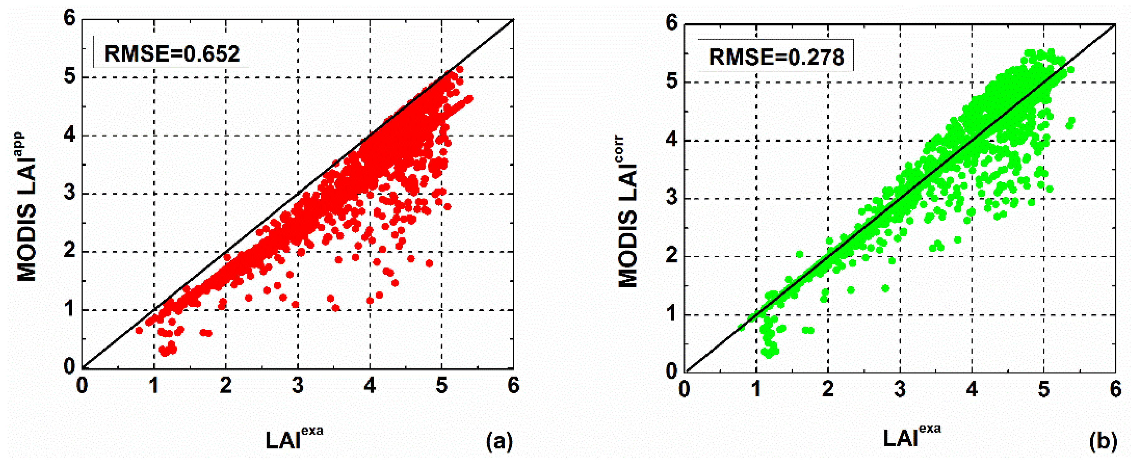
3.4. Validation of LAI Scaling Transfer Method

For the further validation of the availability of the proposed method, the correction of the LAI estimated from the MODIS image (spatial resolution: 250 m) using the developed model was performed. For the spatial one–one correspondence between the up-scaling pixels of CCD image and the original ones of MODIS image, the MODIS image was reprojected and resampled to 240 m, and then the geometric rectification of the MODIS image using the CCD image was conducted. The MODIS LAI^app at the coarse resolution of 240 m was calculated using Equation (1) and then the corrected MODIS LAI^corr was obtained using the proposed LAI scaling transfer model. By comparing the LAI^corr, the LAI^exa, and the LAI^app (Figure 10), the same as with the simulation CCD data in Figure 7, the LAI^app retrieved from the MODIS image were underestimated. Although the correction accuracy of MODIS LAI was low compared with that of the simulation data, the RMSE between the exact LAI LAI^exa estimated from CCD image and the LAI estimated from MODIS image also significantly decreased from 0.652 to 0.278 after correction. Accordingly, the developed method for LAI spatial scaling effect correction based on fractal theory is effective for MODIS LAI correction.

4. Discussion

In accordance with fractal theory, the paper suggested a pixel-based LAI scaling transfer model for correcting the scaling effect by establishing the double logarithmic linear relationship between the fractal dimension D-2 and the NDVI standard deviation σ_NDVI of the up-scaling pixels. The results showed that the scaling transfer model performed well.

In this study, the influence of the spatial heterogeneity of NDVI on the scaling effect of LAI products was mainly considered. However, the spatial scaling effect is caused not only by the spatial heterogeneity of remote sensing data, but also by the nonlinearity of LAI retrieval model [43]. Even if the relationship between the vegetation index (VI) and the LAI were linear, and the spatial distribution of the objects were heterogeneous, there would not be the scaling bias among the LAIs estimated from the different resolution pixels. Furthermore, the scaling bias changes when the nonlinearity type of the empirical regression function used is different [36]. Because the LAI value of the heterogeneous pixel would be overestimated (with the logarithmic regression function), underestimated (with the exponential regression function) or not be affected (with the linear regression function), and therefore it leads to the difference among the scaling bias generated from the same heterogeneous pixel. Therefore, the proposed methodology in this study also depends on the empirical regression function type of the VI and the LAI. In this study, only the exponential function for LAI estimation was analyzed according to the relationship between the measured LAI values and the NDVI values on the sample sites of the study area. The effects of the LAI retrieval model type on LAI scale transformation modeling with fractal theory should be considered in our future work. Besides, the nonlinearity relationship between NDVI and the reflectance of red and near-infrared bands (scaling effect of NDVI) also contributes to the scaling effect of LAI products [31,44,45,46]. Our future work will also further investigate this issue.

Remote sensing products have a property of information fractal [7]. In geometric fractal, the dimension of the ruler or square plane is the same as that of the measured curve or curved surface for computing the geometric fractal dimension [47,48,49]. However, in information fractal, the dimension of the pixel area is not identical to the dimension of the remote sensing products, such as NDVI or LAI value. To express the difference among remote sensing products at different spatial resolutions caused by the scaling effect, we used the remote sensing retrieval results at different spatial resolutions to calculate the information fractal dimension D, which can solve the problem of different dimensions. Given the difference in the computing methods, the ranges of the two types of fractal dimensions are different. For example, the information fractal dimension of the entire CCD image is 2.0088, whereas the geometric fractal dimension of that calculated by the fractal Brownian motion method (FBM) [47] is 2.0552. Although the information fractal dimension of the CCD image is not as large as the geometric fractal dimension, its insignificant variation can cause a great variation in LAIs at different scales. For example, the maximum information fractal dimension of the up-scaling pixel at scale 16 is only 2.0967, whereas the exact LAI value is 1.24 times as large as the approximated LAI value estimated from the coarse resolution pixel (Figure 7).

In this study, the coarse spatial resolution pixels were acquired by aggregating the original high spatial resolution pixels, which means that the up-scaling images share the common imaging characteristics with the original high resolution image. However, the different spatial resolution images captured by different sensors possess the different imaging parameters in reality. Therefore, it is necessary to normalize the imaging parameters of the remote sensing images from different sensors when correcting the LAI scaling effect by using the scaling transfer model in further exploration and study.

5. Conclusions

In analysis and application of remote sensing information, it is necessary to correct the scaling effect of the LAI retrieved from the heterogeneous pixel. Fractal theory offers an efficient and simple tool for spatial scaling effect correction. This study developed a pixel-based LAI scaling transfer model based on fractal theory for correcting the LAI scaling effect. Results indicated that the information fractal dimension D of the up-scaling pixel was closely related to the NDVI standard deviation σ_NDVI of the up-scaling pixel. The LAI scaling transfer model that was established based on the aforementioned relationship performed well in estimating the exact LAI value, with a maximum value of RMSE equaling to 0.011 at different spatial resolutions. The maximum ACE and RCE were only 0.108% and 8.56%, respectively. The standard deviation σ_NDVI (spatial heterogeneity) was the primary cause of the scaling effect and the key influencing factor of the correction effect. The results suggested that the developed method performs well in LAI spatial scaling correction and provides a new perspective for correcting the scaling effect of the other remote sensing products.

References

1. Hilker, T.; Hall, F.G.; Coops, N.C.; Lyapustin, A.; Wang, Y.J.; Nesic, Z.; Grant, N.; Black, T.A.; Wulder, M.A.; Kljun, N.; et al. Remote sensing of photosynthetic light-use efficiency across two forested biomes: Spatial scaling. Remote Sens. Environ. 2010, 114, 2863–2874. [Google Scholar] [CrossRef]
2. Nagler, P.L.; Brown, T.; Hultine, K.R.; van Riper, C.; Bean, D.W.; Dennison, P.E.; Murray, R.S.; Glenn, E.P. Regional scale impacts of Tamarix leaf beetles (Diorhabda carinulata) on the water availability of western US rivers as determined by multi-scale remote sensing methods. Remote Sens. Environ. 2012, 118, 227–240. [Google Scholar] [CrossRef]
3. Raptis, V.S.; Vaughan, R.A.; Wright, G.G. The effect of scaling on land cover classification from satellite data. Comput. Geosci.-UK 2003, 29, 705–714. [Google Scholar] [CrossRef]
4. Chini, M.; Chiancone, A.; Stramondo, S. Scale Object Selection (SOS) through a hierarchical segmentation by a multi-spectral per-pixel classification. Pattern Recogn. Lett. 2014, 49, 214–223. [Google Scholar] [CrossRef] [Green Version]
5. Huang, J.X.; Tian, L.Y.; Liang, S.L.; Ma, H.Y.; Becker-Reshef, I.; Huang, Y.B.; Su, W.; Zhang, X.D.; Zhu, D.H.; Wu, W.B. Improving winter wheat yield estimation by assimilation of the leaf area index from Landsat TM and MODIS data into the WOFOST model. Agric. For. Meteorol. 2015, 204, 106–121. [Google Scholar] [CrossRef]
6. Huang, J.X.; Fernando, S.; Huang, Y.B.; Ma, H.Y.; Li, X.L.; Liang, S.L.; Tian, L.Y.; Zhang, X.D.; Fan, J.L.; Wu, W.B. Assimilating a synthetic Kalman filter leaf area index series into the WOFOST model to improve regional winter wheat yield estimation. Agric. For. Meteorol. 2016, 216, 188–202. [Google Scholar] [CrossRef]
7. Zhang, R.H.; Tian, J.; Li, Z.L.; Su, H.B.; Chen, S.H.; Tang, X.Z. Principles and methods for the validation of quantitative remote sensing products. Sci. China Ser. D 2010, 53, 741–751. [Google Scholar] [CrossRef]
8. Liang, L.; Schwartz, M.D.; Fei, S.L. Validating satellite phenology through intensive ground observation and landscape scaling in a mixed seasonal forest. Remote Sens. Environ. 2011, 115, 143–157. [Google Scholar] [CrossRef]
9. Zhang, H.; Jiao, Z.T.; Yang, H.; Li, X.W.; Wang, J.D.; Su, L.H.; Yan, G.J.; Zhao, H.G. Research on scale effect of histogram. Sci. China Ser. D 2002, 45, 949–961. [Google Scholar] [CrossRef]
10. Sellers, P.J.; Dickinson, R.E.; Randall, D.A.; Betts, A.K.; Hall, F.G.; Berry, J.A.; Collatz, G.J.; Denning, A.S.; Mooney, H.A.; Nobre, C.A.; et al. Modeling the exchanges of energy, water, and carbon between continents and the atmosphere. Science 1997, 275, 502–509. [Google Scholar] [CrossRef] [PubMed]
11. Arora, V. Modeling vegetation as a dynamic component in soil-vegetation-atmosphere transfer schemes and hydrological models. Rev. Geophys. 2002, 40, 1–26. [Google Scholar] [CrossRef]
12. Jonathan, A. Vegetation-Climate Interaction; Springer-Verlag: London, UK, 2010. [Google Scholar]
13. Che, M.L.; Chen, B.Z.; Zhang, H.F.; Fang, S.F.; Xu, G.; Lin, X.F.; Wang, Y.C. A new equation for deriving vegetation phenophase from time series of leaf area index (LAI) data. Remote Sens. 2014, 6, 5650–5670. [Google Scholar] [CrossRef]
14. Friedl, M.A.; Davis, F.W.; Michaelsen, J.; Moritz, M.A. Scaling and uncertainty in the relationship between the NDVI and land surface biophysical variables: An analysis using a scene simulation model and data from FIFE. Remote Sens. Environ. 1995, 54, 233–246. [Google Scholar] [CrossRef]
15. Liang, S.L. Numerical experiments on the spatial scaling of land surface albedo and leaf area index. Remote Sen. Rev. 2000, 19, 225–242. [Google Scholar] [CrossRef]
16. Tian, Y.H.; Woodcock, C.E.; Wang, Y.J.; Privette, J.L.; Shabanov, N.V.; Zhou, L.M.; Zhang, Y.; Buermann, W.; Dong, J.R.; Veikkanen, B.; et al. Multiscale analysis and validation of the MODIS LAI product: I. Uncertainty assessment. Remote Sens. Environ. 2002, 83, 414–430. [Google Scholar] [CrossRef]
17. Chen, J.; Ni, S.X.; Li, J.J.; Wu, T. Scaling effect and spatial variability in retrieval of vegetation LAI from remotely sensed data. Acta Ecol. Sin. 2006, 26, 1502–1508. [Google Scholar]
18. Zhu, X.H.; Feng, X.M.; Zhao, Y.S.; Song, X.N. Scale effect and error analysis of crop LAI inversion. J. Remote Sens. 2010, 14, 586–592. [Google Scholar]
19. Artan, G.A.; Neale, C.M.U.; Tarboton, D.G. Characteristic length scale of input data in distributed models: implications for modeling grid size. J. Hydrol. 2000, 227, 128–139. [Google Scholar] [CrossRef]
20. Fernandes, R.A.; Miller, J.R.; Chen, J.M.; Rubinstein, I.G. Evaluating image-based estimates of leaf area index in boreal conifer stands over a range of scales using high-resolution CASI imagery. Remote Sens. Environ. 2004, 89, 200–216. [Google Scholar] [CrossRef]
21. Tian, Q.J.; Jin, Z.Y. Research on calculation and spatial scaling of forest leaf area index from remote sensing image. Remote Sen. Inform. 2006, 4, 5–11. [Google Scholar]
22. Jin, Z.; Tian, Q.; Chen, J.M.; Chen, M. Spatial scaling between leaf area index maps of different resolution. J. Environ. Manage. 2007, 85, 628–637. [Google Scholar] [CrossRef] [PubMed]
23. Liu, Y.; Wang, J.D.; Zhou, H.M.; Xue, H.Z. Upscaling approach for validation of LAI products derived from remote sensing observation. J. Remote Sens. 2014, 18, 1189–1198. [Google Scholar]
24. Hu, Z.; Islam, S. A framework for analyzing and designing scale invariant remote sensing algorithms. IEEE Trans. Geosci. Remote Sens. 1997, 35, 747–755. [Google Scholar]
25. Garrigues, S.; Allard, D.; Baret, F.; Weiss, M. Influence of landscape spatial heterogeneity on the non-linear estimation of leaf area index from moderate spatial resolution remote sensing data. Remote Sens. Environ. 2006, 105, 286–298. [Google Scholar] [CrossRef]
26. Raffy, M. Change of scale in models of remote sensing: a general method for spatialization of models. Remote Sens. Environ. 1992, 40, 101–112. [Google Scholar] [CrossRef]
27. Chen, J.M. Spatial scaling of a remotely sensed surface parameter by contexture. Remote Sens. Environ. 1999, 69, 30–42. [Google Scholar] [CrossRef]
28. Xu, X.R.; Fan, W.J.; Tao, X. The spatial scaling effect of continuous canopy leaves area index retrieved by remote sensing. Sci. China Ser. D 2009, 52, 393–401. [Google Scholar] [CrossRef]
29. Kim, G.; Barros, A.P. Downscaling of remotely sensed soil moisture with a modified fractal interpolation method using contraction mapping and ancillary data. Remote Sens. Environ. 2002, 83, 400–413. [Google Scholar] [CrossRef]
30. Chen, Y.; Chen, L. Fractal Geometry; Earthquake Press: Beijing, China, 2005. [Google Scholar]
31. Luan, H.J.; Tian, Q.J.; Yu, T.; Hu, X.L.; Huang, Y.; Du, L.T.; Zhao, L.M.; Wei, X.; Han, J.; Zhang, Z.W.; et al. Modeling continuous scaling of NDVI based on fractal theory. Spectrosc. Spect. Anal. 2013, 33, 1857–1862. [Google Scholar]
32. Li, X.W.; Wang, J.D.; Strahler, A.H. Scale effect of Planck’s law over nonisothermal blackbody surface. Sci. China Ser. E 1999, 42, 652–656. [Google Scholar] [CrossRef]
33. Su, L.H.; Li, X.W.; Huang, Y.X. An review on scale in remote sensing. Adv. Earth Sci. 2001, 16, 544–548. [Google Scholar]
34. Xu, X.R. Physical Principles of Remote Sensing; Peking University Press: Beijing, China, 2005. [Google Scholar]
35. Liu, C.H. Remote Sensing Inversion of Crop Leaf Area Index Spatial Scale Transformation Modeling Study. Master’s Thesis, China University of Geosciences (Beijing), Beijing, China, 2013. [Google Scholar]
36. Jiang, J.L.; Liu, X.N.; Liu, C.H.; Wu, L.; Xia, X.P.; Liu, M.L.; Du, Z.H. Analyzing the spatial scaling bias of rice leaf area index from Hyperspectral data using wavelet-fractal technique. IEEE J. Sel. Top. Appl. Remote Sens. 2014, 8, 3068–3080. [Google Scholar] [CrossRef]
37. Wu, L.; Liu, X.N.; Zheng, X.P.; Qin, Q.M.; Ren, H.Z.; Sun, Y.J. Spatial scaling transformation modeling based on fractal theory for the leaf area index retrieved from remote sensing imagery. J. Appl. Remote Sens. 2015, 9, 096015. [Google Scholar] [CrossRef]
38. Rouse, J.W.; Haas, R.H.; Schell, J.A.; Deering, D.W. Monitoring vegetation systems in the Great Plains with ERTS-1. In Proceeding of the Third Earth Resources Technology Satellite Symposium, Washington, DC, USA, 10–14 December 1973; pp. 309–317.
39. Mandelbrot, B. How long is the coast of Britain. Science 1967, 156, 636–638. [Google Scholar] [CrossRef] [PubMed]
40. Penland, A.R.; Picard, W.; Sclaroff, S. Photobook: Content based manipulation of image databases. Int. J. Comput. Vis. 1996, 18, 233–254. [Google Scholar] [CrossRef]
41. Mandelbrot, B. The Fractal Geometry of Nature; Freeman: San Francisco, CA, USA, 1982. [Google Scholar]
42. Chen, S.S.; Keller, J.M.; Crownover, R.M. On the calculation of fractal features from images. IEEE Trans. Pattern Anal. 1993, 15, 1087–1090. [Google Scholar] [CrossRef]
43. Fan, W.J.; Gai, Y.Y.; Xu, X.R.; Yan, B.Y. The spatial scaling effect of the discrete-canopy 1 effective leaf area index retrieved by remote sensing. Sci. China Ser. D 2013, 56, 1548–1554. [Google Scholar] [CrossRef]
44. Jiang, Z.Y.; Huete, A.R.; Chen, J.; Chen, Y.H.; Li, J.; Yan, G.J.; Zhang, X.Y. Analysis of NDVI and scaled difference vegetation index retrievals of vegetation fraction. Remote Sens. Environ. 2006, 101, 366–378. [Google Scholar] [CrossRef]
45. Obata, K.; Wada, T.; Miura, T.; Yoshioka, H. Scaling effect of area-averaged NDVI: Monotonicity along the spatial resolution. Remote Sens. 2012, 4, 160–179. [Google Scholar] [CrossRef]
46. Liu, L.Y. Simulation and correction of spatial scaling effects for leaf area index. J. Remote Sens. 2014, 18, 1158–1168. [Google Scholar]
47. Yu, Z.F.; Lin, Z.J. arithmetic research of fractal dimension with image face based on fractional Brownian motion. Geomat. Inf. Sci. Wuhan Univ. 2005, 30, 161–165. [Google Scholar]
48. Chaudhuri, B.B.; Sarkar, N. Texture segmentation using fractal dimension. IEEE Trans. Pattern Anal. 1995, 17, 72–77. [Google Scholar] [CrossRef]
49. Jaggi, S.; Quattrochi, D.A.; Lam, N.S.N. Implementation and operation of 3 fractal measurement algorithms for analysis of remote-sensing data. Comput. Geosci.-UK 1993, 19, 745–767. [Google Scholar] [CrossRef]
Figure 1. Location of the study area and the charge-coupled device (CCD) image used in this study. The CCD image (RGB = G (0.52 μm to 0.60 μm), NIR (0.76 μm to 0.90 μm), and R (0.63 μm to 0.69 μm)) is of the study area in Changchun, China. The sample sites for modeling are shown as red stars.
Remotesensing 08 00197 g001
Figure 2. Mapping of leaf area index (LAI) from CCD image: (a) empirical regression function f relating LAI to normalized difference vegetation index (NDVI); (b) NDVI data generated from CCD image; and (c) LAI distributions mapped from NDVI data.
Remotesensing 08 00197 g002
Figure 3. Two up-scaling methods of LAI retrieval (cited from [25]): f is an empirical regression function relating LAI to the vegetation index (VI); VIi (i = 1, 2, 3, 4) is the VI value of the original high resolution pixel and LAIi is the corresponding LAI value; LAIexa, the exact LAI value of the coarse resolution pixel, is calculated by averaging all the LAIi results within the coarse resolution pixel (i = 1, 2, 3, 4); VIm (i.e., the average of VIi) represents the VI value of the coarse spatial resolution pixel; and LAIapp, calculated by applying f to VIm, is the approximated LAI value of the coarse resolution pixel.
Remotesensing 08 00197 g003
Figure 4. Relationships between the transformation form of the information fractal dimension D-2 and the NDVI standard deviation σNDVI of the up-scaling pixels with different sizes. The sizes of the pixels are: (a) 4 × 4; (b) 8 × 8; (c) 16 × 16; and (d) 32 × 32 original pixels.
Remotesensing 08 00197 g004
Figure 5. Double logarithmic diagram of the transformation form of the fractal dimension D-2 and the NDVI standard deviation σNDVI of the up-scaling pixels with different sizes. The sizes of the up-scaling pixels are: (a) 4 × 4; (b) 8 × 8; (c) 16 × 16; and (d) 32 × 32 original pixels.
Remotesensing 08 00197 g005
Figure 6. Analysis of the absolute scaling bias (ASB) and the relative scaling bias (RSB) of the up-scaling pixels (e.g., the up-scaling pixels of size 16 × 16 original pixels): (a) the relationship between ASB and σNDVI (or D); and (b) the relationship between RSB and σNDVI (or D).
Remotesensing 08 00197 g006
Figure 7. Correction of the scaling effect of the LAI estimated from the coarse remote sensing images at different spatial resolutions. The sizes of the pixels are: (a) 4 × 4; (b) 8 × 8; (c) 16 × 16; and (d) 32 × 32 original pixels. LAIexa is the exact LAI; LAIapp is the approximated LAI before correction; and LAIcorr is the corrected LAI.
Remotesensing 08 00197 g007
Figure 8. Relationships between the absolute correction error (ACE) (or relative correction error (RCE)) and σNDVI of the up-scaling pixels with different sizes. The sizes of the up-scaling pixels are: (a,b) 4 × 4; (c,d) 8 × 8; (e,f) 16 × 16; and (g,h) 32 × 32 original pixels.
Remotesensing 08 00197 g008aRemotesensing 08 00197 g008b
Figure 9. Relationships between the exact LAI value LAIexa and σNDVI of the up-scaling pixels with different sizes. The sizes of the up-scaling pixels are: (a) 4 × 4; (b) 8 × 8; (c) 16 × 16; and (d) 32 × 32 original pixels.
Remotesensing 08 00197 g009
Figure 10. Verification of the LAI scaling transfer model applicability to the MODIS image with the spatial resolution of 250 m. MODIS LAI (a) before and (b) after correction.
Remotesensing 08 00197 g010