Article

Noise Localization Method for Model Tests in a Large Cavitation Tunnel Using a Hydrophone Array

1
Advanced Ship Research Division, Korea Research Institute of Ships & Ocean Engineering, Daejeon 34103, Korea
2
Department of Defense Systems Engineering, Sejong University, Seoul 143-747, Korea
3
Department of Naval Architecture and Ocean Engineering, Seoul National University, Seoul 151-744, Korea
*
Author to whom correspondence should be addressed.
Remote Sens. 2016, 8(3), 195; https://doi.org/10.3390/rs8030195
Submission received: 3 December 2015 / Revised: 21 January 2016 / Accepted: 24 February 2016 / Published: 27 February 2016
(This article belongs to the Special Issue Underwater Acoustic Remote Sensing)

Abstract

:
Model tests are performed in order to predict the noise level of a full ship and to control its noise signature. Localizing noise sources in the model test is therefore an important research subject along with measuring noise levels. In this paper, a noise localization method using a hydrophone array in a large cavitation tunnel is presented. The 45-channel hydrophone array was designed using a global optimization technique for noise measurement. A set of noise experiments was performed in the KRISO (Korea Research Institute of Ships & Ocean Engineering) large cavitation tunnel using scaled models, including a ship with a single propeller, a ship with twin propellers and an underwater vehicle. The incoherent broadband processors defined based on the Bartlett and the minimum variance (MV) processors were applied to the measured data. The results of data analysis and localization are presented in the paper. Finally, it is shown that the mechanical noise, as well as the propeller noise can be successfully localized using the proposed localization method.

Graphical Abstract

1. Introduction

In order to reduce shipping noise, the characteristics of ship noise should be understood. Localizing the noise sources in the design stage via an indirect method, such as acoustic sensing, as well as visual observation might be very helpful for this purpose.
Propeller noise, which is one of the main noise sources in ships, is mainly due to its turns as spectral harmonics and to cavitation as broadband noise. Thus, research has focused on propeller cavitation theoretically and experimentally. Experimental studies of cavitation noise have been performed to meet various objectives, including detecting the inception and extent of cavitation, identifying noise characteristics with respect to cavitation behaviors and predicting cavitation noise levels [1,2,3,4,5,6]. In contrast to the full-scale measurements where noise components coming from other sources, such as a loud engine, are inevitably included, the measurement of noise levels generated by rotating propellers exclusively is possible in the cavitation tunnel experiments. However, since the noise levels measured at the cavitation test facility are model scaled, the full-scale noise levels are approximated through scaling laws [7,8,9,10,11]. In the noise tests, it is important to set up the proper test procedure for reliable measurements and analysis of the noise data. Therefore, one of the main concerns of the cavitation noise study was establishing the measuring techniques or procedures appropriate for each type of facility configuration [7,12,13,14,15,16,17].
The noise measurements in the cavitation tunnel are performed using single hydrophone or/and a hydrophone array. A single hydrophone measurement is usually utilized when the level of signals, i.e., propeller noise, is larger than the background noise due to its easy implementation. However, it is not applicable when the level of signals is comparable to, or lower than, the background noise. This limitation can be overcome by using the hydrophone array and its array gain. Most large cavitation tunnels where model tests are possible using a model ship with appendages are equipped with the array system [18,19,20]. The hydrophone array is generally installed inside the acoustic trough, which is isolated from the test section by acoustic windows in order to reduce the effect of flow noise.
Utilization of the hydrophone array is inevitable for array signal processing, such as beamforming [21] and matched field processing (MFP) [22]. Beamforming has been widely used to detect and localize an acoustic source in the ocean. However, the multi-path reflections can degrade the accuracy of beamforming. In order to overcome this drawback, MFP has been widely investigated in the underwater acoustics research community [22,23]. Since MFP fully utilizes the acoustic field, including multi-path components, it is adequate for shallow water applications. In principle, there is no difference between MFP and beamforming, except for utilizing the spatial complexity [23]. The conventional beamforming is still widely used in the airborne application, such as noise localization in a wind tunnel [24].
Park et al. [25] localized the propeller cavitation noise using the 10-channel hydrophone array vertically configured inside the test section of the small cavitation tunnel. MFP was used as the localization method, and the replica fields were directly measured using a virtual source. Chang et al. [26,27] localized vortex cavitation utilizing the time difference of arrival (TDOA). The experiment was performed in a small-sized water tunnel with a number of hydrophones in multiple configurations. Anderson [28] localized the laser-induced cavitation in a twelve-inch diameter water tunnel using hydrophones of different array configurations. A number of localization methods including MFP were tested in the localizations. For the MFP, a replica field was simulated by a ray-based model accounting for the effects of multiple reflections in the test section. Lee et al. [29] used narrowband matched field inversion (MFI) in order to model the propeller sheet cavitation noise source. The boundary element method (BEM) was used for the calculation of the replica pressure field, and the dominant one blade passage frequency (BPF) components of the received signals were used in the localization process. Kim et al. [30] performed similar research for the modeling of non-cavitating propeller noise. Recently, Kim et al. [31] suggested a ray-based MFI method for the localization of incipient tip vortex cavitation using nearfield data measured at the hydrophones flush mounted on the hull of a model ship. They used ray-based simulation for the calculation of the replica field. Felli et al. [32] performed an experimental study on the propeller-induced perturbation on the rudder. They directly measured the pressure field over the rudder surface behind the propeller using a set of flush-mounted transducers in order to identify the perturbation sources affecting the propeller-rudder interaction.
At our institute, KRISO, a large cavitation tunnel is operated, which has a low background noise characteristic for the noise test. We performed a set of experiments for measuring and localizing propeller noise using a 45-channel hydrophone array, which is installed inside the acoustic trough. In this paper, the experiments are described, and the results are presented. We defined two objective functions for the broadband source localizations and applied them to the noise data from various sources, such as a virtual source, cavitating propellers, non-cavitating propellers, a singing propeller and a driving motor. Section 2 describes the noise experiment performed in the KRISO cavitation tunnel and the array signal processing method. Section 3 presents the results and discussion. Finally, the summary and conclusion are given in Section 4.

2. Methods

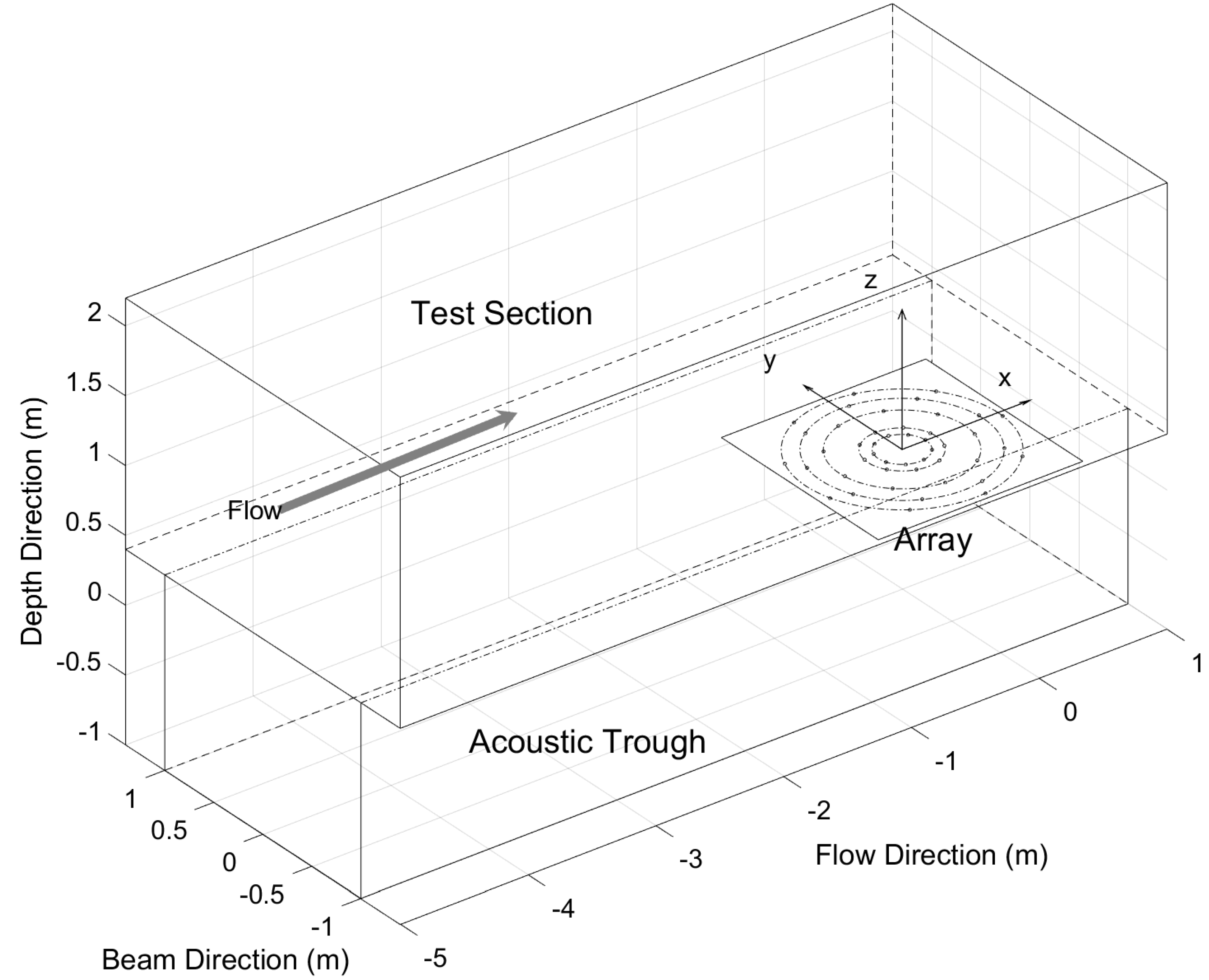
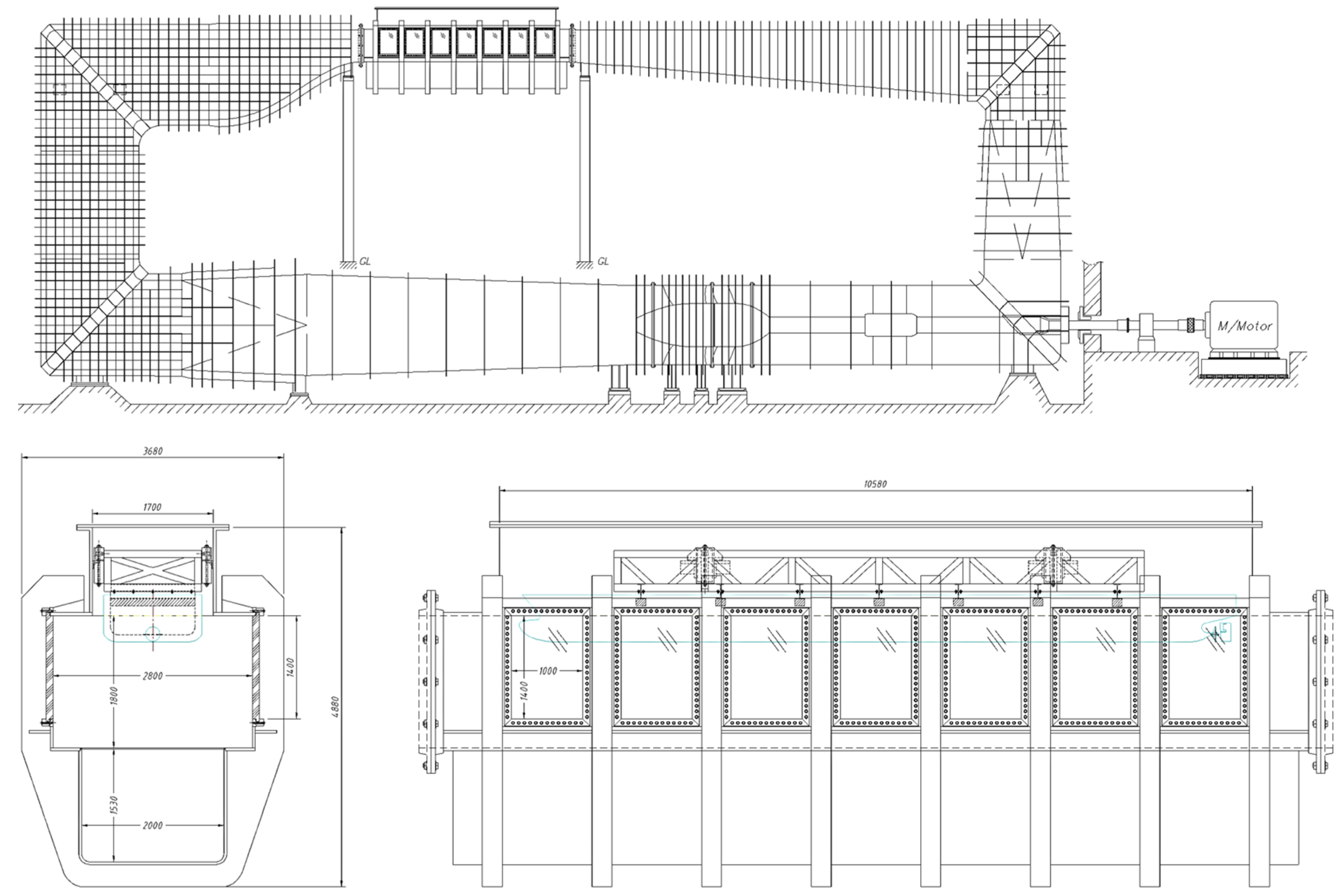
2.1. Description of Model Tests

The propeller noise measurement experiments were performed in the KRISO large cavitation tunnel. The objectives of the experiment were to measure and analyze the noise generated by a set of model propellers and model ships. The cavitation tunnel has a rectangular test section, which is 12.5 m (L) × 2.8 m (B) × 1.8 m (H). In the test section, a model ship of a maximum length of 12 m can be installed. The maximum flow speed is 16.5 m/s, and the pressure can be adjusted from 0.02 to 3.5 bar. A schematic diagram of the large cavitation tunnel is shown in Figure 1.
The main function of the cavitation tunnel is observing the cavitation patterns of the model propellers. Therefore, it is important to set the flow around the model propeller similarly to that of a full-scale ship. The large cavitation tunnel has the advantage of easily satisfying the flow similarity using a fully-fitted model ship. The large cavitation tunnel is also suitable for noise measurement experiments, since it does not require the wake screen usually used for simulating the ship’s wake flow in a small cavitation tunnel, thus generating unwanted noise. However, the scale effect still exists due to the discrepancy of the Reynolds number between the full-scale and the model. It can alter the ship wake, thus changing the cavitation behavior. In addition, the inception of the tip vortex, which is the main source of noise for naval ships, mega-yachts and cruise ships, is strongly affected by the Reynolds scale effect [3,11]. In order to reduce its effects on the model test, various techniques, such as utilizing a dummy body to simulate the estimated full-ship wake and artificial increasing of leading edge roughness to avoid laminar boundary flow, can be applied. However, no modifications were applied in the model tests in this paper.
The measuring system consists of a hydrophone array, signal conditioning amplifiers and a data acquisition unit. The hydrophone was the B&K 8103, which has a flat frequency response over the range of 0.1 Hz to 180 kHz with a nominal receiving sensitivity of −211 dB re 1 V/μPa [33]. The B&K NEXUS Type 2692 was used as a conditioning amplifier, and signals were acquired by the B&K PULSE analyzer platform. The array was installed inside the acoustic trough, as shown in Figure 2. The acoustic window separates the acoustic trough from the test section where the models are installed and the water flows. Sound-absorbing materials are installed on the trough walls in order to reduce inside reverberations. A Lexan plate with dimensions of 1.6 m × 1.6 m is used as a signal conditioning plate to securely fix the hydrophones at the designed positions of the array. The configuration of the array was determined via an optimization technique, which is comprised of design parameters, an objective function and an optimization algorithm [34]. The design parameters were defined for variously-shaped planar arrays. The objective function was defined in order to consider the main lobe beam width and the maximum side lobe level simultaneously. A global optimization scheme was applied to the array design using very fast simulated reannealing (VFSR). After applying the optimization technique to the arrays, respectively, the optimum shape was chosen for the 45-channel array. The designed array comprises 5 concentric circles of which the radii vary from 0.18 m to 0.75 m. In each circle, 9 hydrophones are evenly spaced around the circle, and the azimuth angle of the reference hydrophone was decided by the optimization. The array faces upward, as shown in Figure 2. The vertical distance from the center of the array to the top of the test section is 2.2 m. Figure 3 shows beam patterns for the selected direction of arrival (DoA) when the array is uniformly weighted [21]. The beam patterns are calculated for the elevation angle with respect to the z-axis from −90° to 90°, while the azimuth angle from the x-axis is set to 0° (see Figure 2). The direction of arrival also refers to the elevation angle with the azimuth angle of 0°.
The propeller noise was measured during the cavitation observation tests. The test conditions were determined using the thrust identity method at a specified self-propulsion point [1]. In the cavitation tests, the propeller operating condition is defined by the non-dimensional coefficients, propeller thrust coefficient K T and cavitation number σ n , which are defined as follows.
K T = 16 T ρ n 2 R 4
σ n = 8 ( p 0 p v ) ρ n 2 R 2
where ρ is the water density, n is the propeller rotational speed per second and R is the radius of the propeller. In addition, T refers to the thrust of the propeller, and p 0 and p v represent the static and vapor pressures, respectively. During the propeller cavitation observations and noise measurements, the pressure in the cavitation tunnel is adjusted according to the local cavitation number at the point approximating the center of the expected cavitation extent.
Background noise was also measured in the experiments. Background noise refers to noise from all sources other than the source being tested, i.e., propeller cavitation. The background noise derives mainly from the propeller drive system, the tunnel operation, the water flow, the measurement chain, etc. To check the quality of the noise measurements, i.e., of the propeller, the background noise level should be measured and specified. According to [35], the background noise can be measured in absence of the propeller cavitation, but with all other operating conditions similar to those in the propeller noise measurement. The cavitation can be removed by replacing the propeller by a dummy boss or by increasing tunnel pressure to suppress it. Both methods to measure background noise have pros and cons. The increase of tunnel pressure allows one to keep the propeller load condition, K T , and to detect propeller non-cavitating noise (e.g., propeller singing), but changes the air content. It also removes or at least reduces the cavitation from the appendages of the ship model, which should be included in the background noise if it exists. The replacement of the propeller by a dummy boss keeps the same air content, but changes the load of the propeller drive system. Thus, it would alter the mechanical noise characteristics from the propeller drive system. We adopted the method to replace the propeller by a dummy boss.
In the above procedure, the sound pressure level (SPL) is obtained by converting the measured acoustic pressures into decibels. In order to obtain the source level (SL) from the SPL, we need to measure or estimate the transfer function between the source and the receiver. For the transfer function measurement, the propeller was replaced by a known source, which is called the virtual source. The underwater transducer ITC-1032, which converts the electrical input to the pressure signal with its own transmitting voltage response (TVR), was used as the virtual source. ITC-1032 has a resonance frequency ( f r ) of 33 kHz, and its TVR at f r is 149 dB//μPa/V @ 1 m [36]. The source strength of the virtual source can be calculated directly from the known input signal (voltage) and TVR. The white noise generated by a function generator (Agilent33500B) was used as the input signal. Other signals, such as the chirp signal [37], can be used for the virtual source, as well. The input signal fully covered the frequency range of interest (1 to 100 kHz). The localization of the virtual source will also be used as a reference position to check the validity of the other source localization results, such as propeller cavitations.

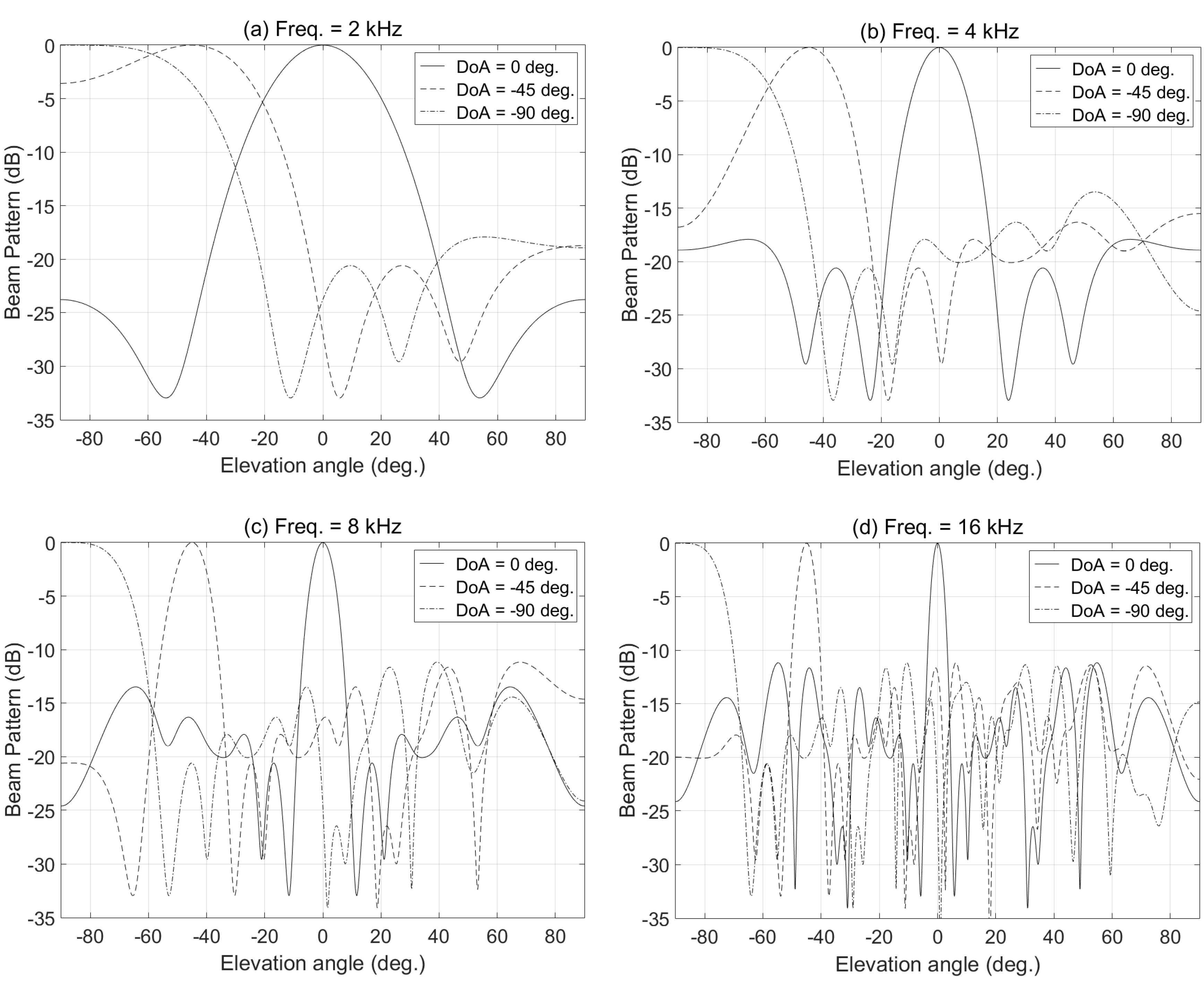
2.2. Array Signal Processing for Source Localization

The acoustic data measured from a rotating propeller behind a body, such as a ship or submarine, comprises signals of interest propagated from the propeller and additional noise due to other sources, such as unsteady flows along the body surface or/and tunnel walls and the inherent electrical noise of measuring devices. If we consider a specific source, the measured data d ( t ) can be modeled by the following equation, since the propagation of the source signal s ( t ) through the medium can be expressed by convolution with an impulse response h ( t ) in a linear time-invariant system [38].
d ( r , t ) = s ( r s , t ) * h ( r , r s , t ) + n ( r , t )
In Equation (3), * refers to the convolution operator; r and r s represent the receiver and source positions, respectively; and n ( t ) is the additional noise signal. If more sources exist, the corresponding terms can be simply added to Equation (3). Applying Fourier transform to Equation (3), the frequency domain expression for the angular frequency ω becomes:
D ( r , ω ) = S ( r s , ω ) H ( r , r s , ω ) + N ( r , ω )
For an array of M receivers, the measured noise field at all receiver points can be expressed by vector D = [ D 1 , D 2 , , D M ] T . Similarly, we can construct a replica field vector H = [ H ^ 1 , H ^ 2 , , H ^ M ] T . Replica fields are usually obtained by the numerical simulation of transfer functions. The transfer function of the tunnel can be modeled as:
H ^ ( r , r s , ω ) = k = 1 A k ( r , r s , ω ) e i k ( r , r s , ω )
Equation (5) represents multiple arrivals with different amplitudes ( A ) and phases ( ). Figure 4a shows an example of Green’s functions for the 45 receivers obtained using a virtual source. The virtual source was located at the positions of (0.1 m, 0 m, 1.9 m) relative to the array center, and the frequency range of the input signal was from 1 kHz to 100 kHz. From the figure, multiple reflections along with strong direct arrivals are observed. Figure 4b shows the simulated Green’s function, where such arrivals are included as follows: D, direct arrival; DB, array plate (bottom)-reflected arrival; DBm, multiple reflections between the acoustic window and array plate; S, surface-reflected arrival; SB, surface-bottom-reflected arrival; W, wall-reflected arrival; WB, wall-bottom-reflected arrival; SW, surface-wall-reflected arrival; and SWB, surface-wall-bottom-reflected arrival. Green’s function is calculated using a ray tracing method. The eigenrays representing multiple reflections are shown in Figure 4c. The detail of the bottom-reflected arrival is also given in the figure. The standoff distance in the plot is 15.8 mm for B&K 8103 [33]. Comparing Figure 4a,b, it can be seen that (i) the surface- and wall-reflected arrivals are not distinct in the measured data and (ii) multiple reflections from unknown reflectors exist. Thus, it is very difficult to simulate the transfer function exactly, so we approximate it using only a direct arrival as:
H ^ ( r , r s , ω ) = 1 | r r s | e i ω | r r s | c 0
where | r r s | is the distance between the source and the receiver and c 0 is the sound speed. Kim et al. [31] used the direct arrivals for the localization of the tip vortex cavitation. In addition, source localization results using multiple reflections were not better than those obtained using direct arrivals only, as can be seen in Subsection 3.1.
Cross-correlating the measured field with the replica leads to the Bartlett processor that evaluates the similarity between structures of two acoustic fields [22]. If the positions of the virtual source and actual source coincide, the processor will show the highest correlation value, since the measured field vector and the replica field vector should be similar. To incorporate the broadband nature of the propeller cavitation noise, an incoherent broadband processor is given as the first objective function as follows:
Φ B ( r ^ s ) = 1 N f j = 1 N f w B + ( r , r ^ s , ω j ) C ( r , ω j ) w B ( r , r ^ s , ω j )
where:
w B ( r , r ^ s , ω ) = H ^ ( r , r ^ s , ω ) H ^ ( r , r ^ s , ω ) , C ( r , ω j ) = D ( r , ω ) D ( r , ω ) + D ( r , ω ) 2
In Equation (7), C and w B represent the cross-spectral data matrix and the weight vector of the Bartlett processor, respectively. In addition, w + refers to the transpose of the complex vector   w , while r ^ s is a candidate source position. a is the L 2 norm of a vector a , and b is the expected value of b .
Similarly, the incoherent broadband processor using the minimum variance (MV) processor is given as the second objective function as follows:
Φ M V ( r ^ s ) = 1 N f j = 1 N f ( w B + ( r , r ^ s , ω j ) C 1 ( r , ω j ) w B ( r , r ^ s , ω j ) ) 1
where C 1 is the inverse matrix of C .
The MV processor has both pros and cons at the same time. It is optimum in the sense that the output noise power is minimized subject to the constraint that the signal be undistorted by the processor [22]. It can achieve the best localization performance under the ideal conditions, such as a large signal-to-noise ratio (SNR) and without mismatch. However, the source of errors, such as an inaccurate array position, and the discrepancy between the measured signal and the replica can degrade its performance significantly.
The MFP utilizes both amplitude and the phase. However, it is more sensitive to the phase than the amplitude. The spatial resolution is one of the main parameters to evaluate the array performance. In order to get insight into it, a simulation study is performed regarding the source-array configuration, which decides the phase in Equation (6). The spatial resolution can be evaluated by the half power beam width (HPBW), which is defined by the distance between the candidate points ( r ^ s ), where Φ ( r ^ s ) / Φ ( r s ) = 0.5 , as shown in Figure 5a. For simplicity’s sake, a monopole source in the free field is used in the simulation. The source is assumed to be located at r s = ( x s ,   0.0   m , 1.3 m ) , where 2.0 m x s   2.0   m .
Figure 5b,c shows the simulation results for the Bartlett and the MV processor, respectively, under the condition of 8 kHz and 0 dB SNR. The x-directional HPBW ( HPBW x ) increases monotonically as the source moves from the array center, i.e., broadside. The HPBW y also shows a monotonic increase, but the change is gradual. However, the HPBW z decreases up to x s ± 1.1 m and increases again after passing the point. Comparing two processors, the MV processor shows better resolution than the Bartlett processor, since there is no mismatch in the simulation.
The different behaviors of the spatial resolution can be explained by the phase difference depending on the source-array configuration. If we consider a source at r s and two different receivers at r 1 and r 2 , the phase difference ( Δ φ ) becomes k ( | r 1 r s | | r 2 r s | ) , where k is the wavenumber. The phase sensitivity, which refers to the effect of the change of the source position in a direction on the phase difference, is defined by | Δ φ | r s | | . Assuming two receiver positions as (−0.1 m, 0 m, 0 m) and (0.1 m, 0 m, 0 m), the phase sensitivity with respect to the source position is shown in Figure 5d. Comparing the HPBW in Figure 5b,c and the phase sensitivity in Figure 5d, it is clear that the fine spatial resolution is achieved at the source position around where the phase difference changes significantly.

3. Results and Discussion

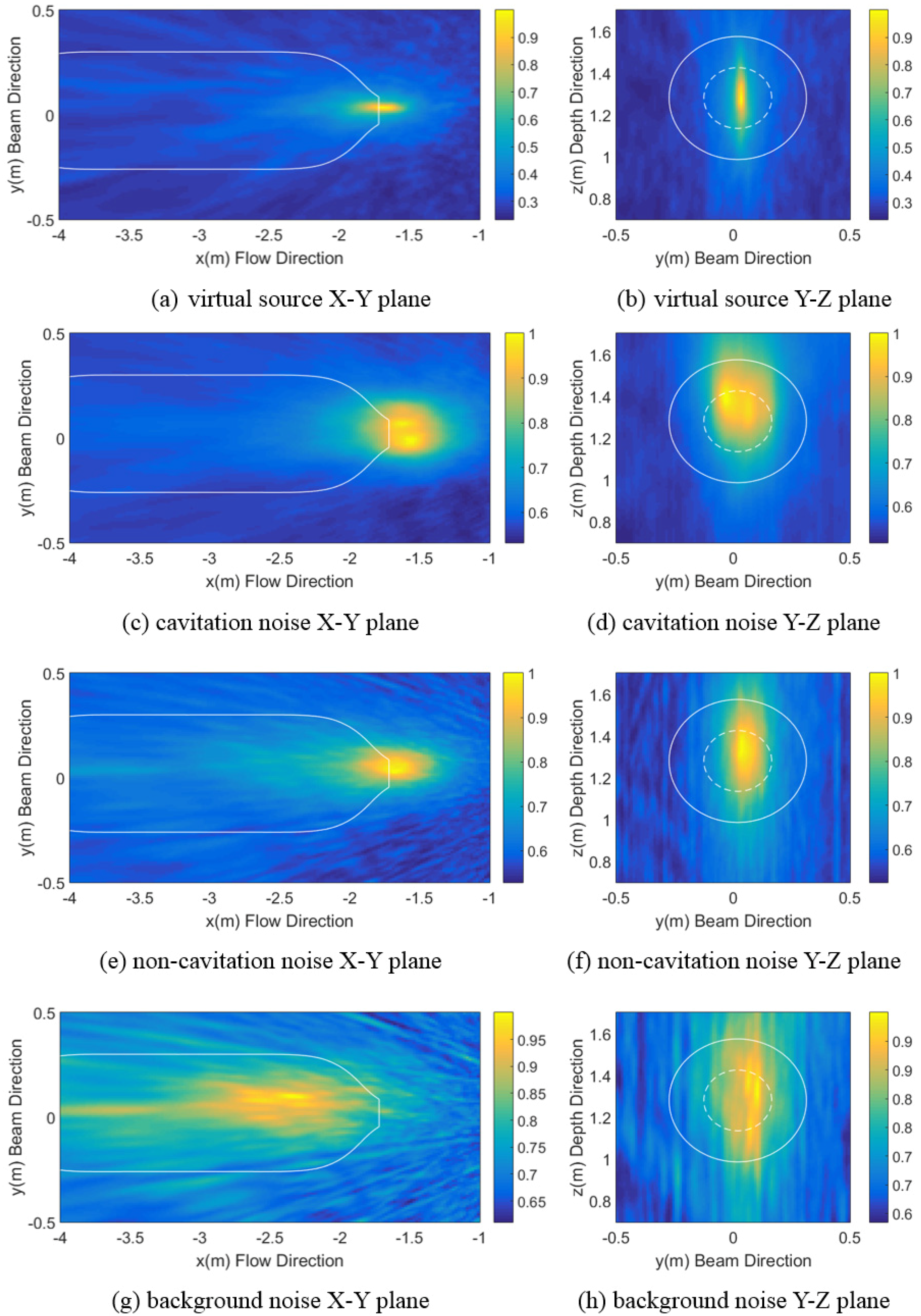
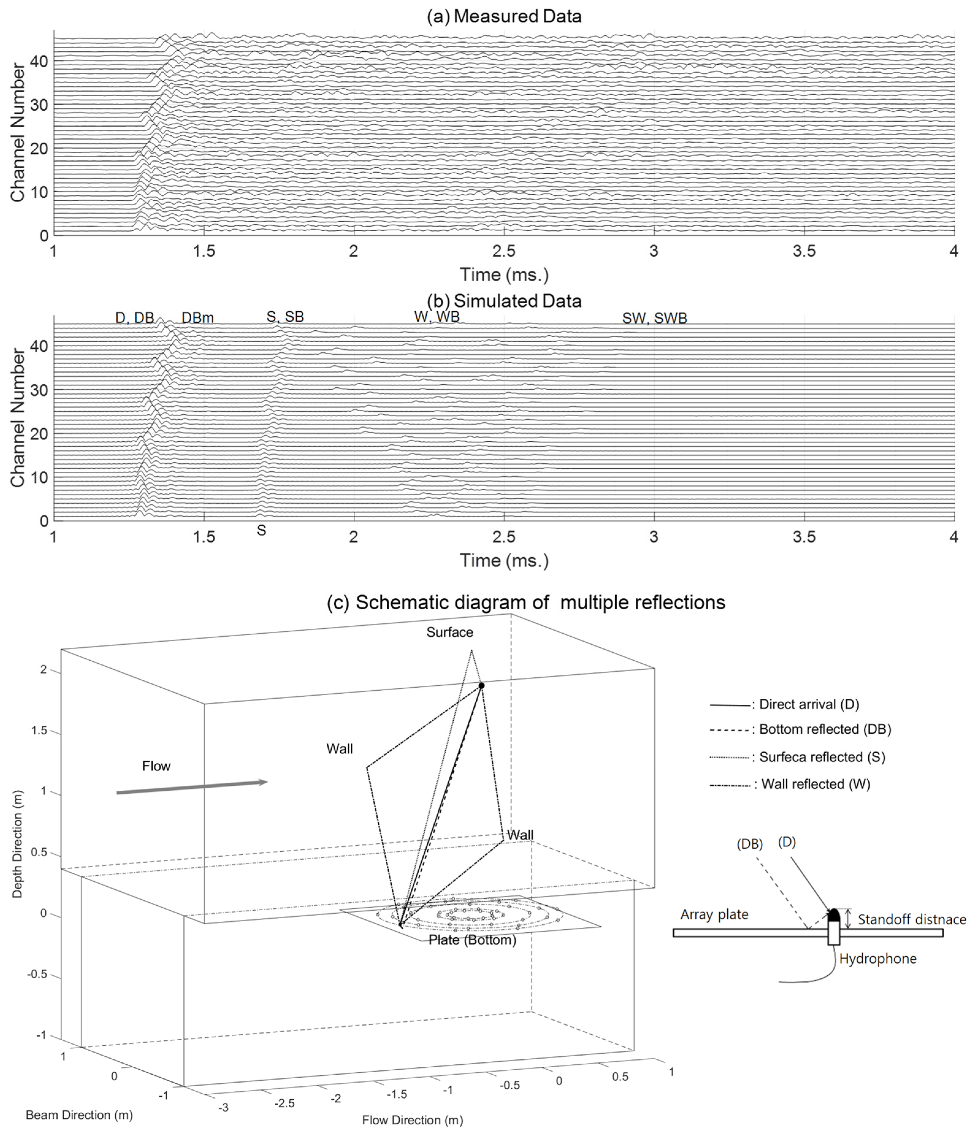
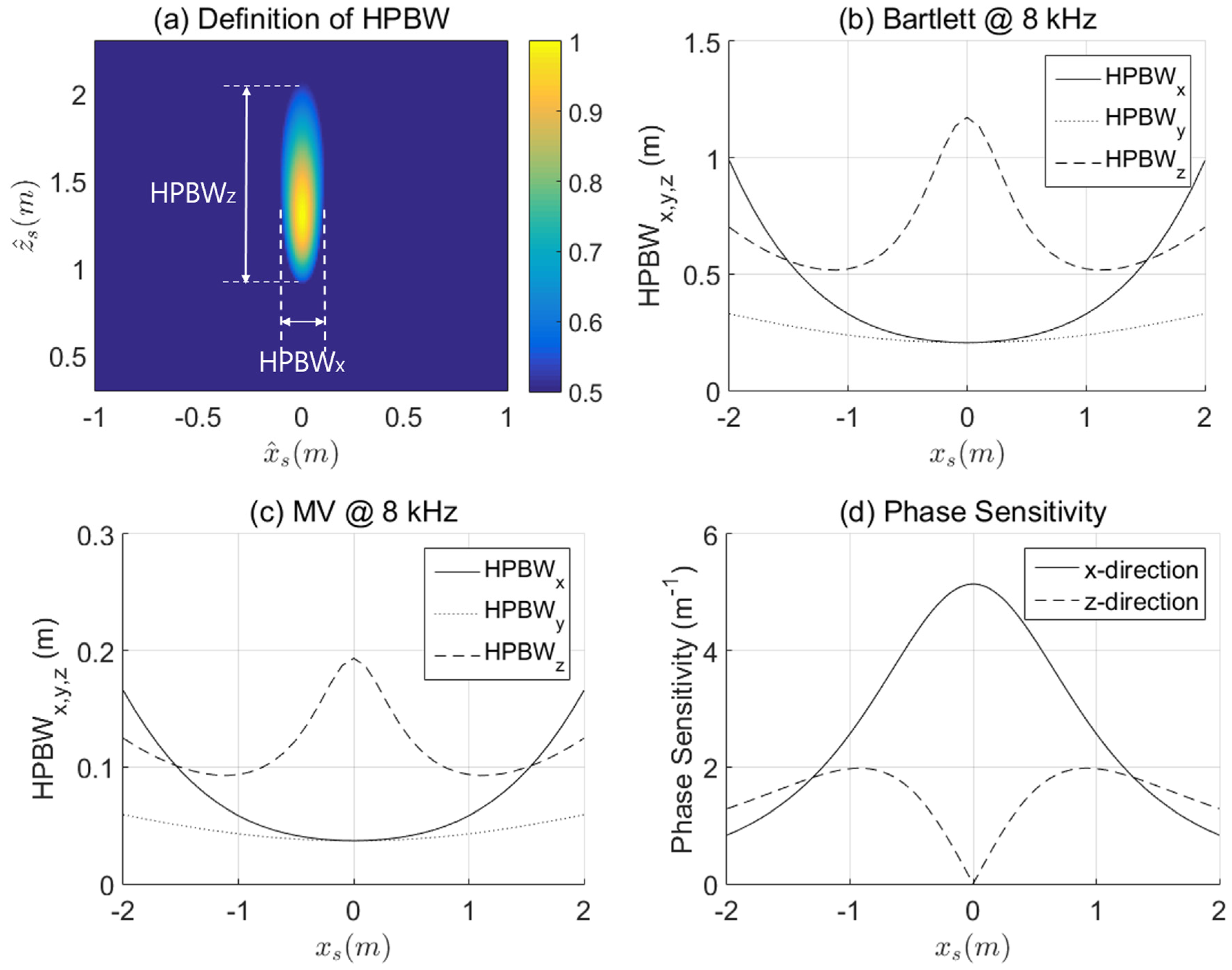
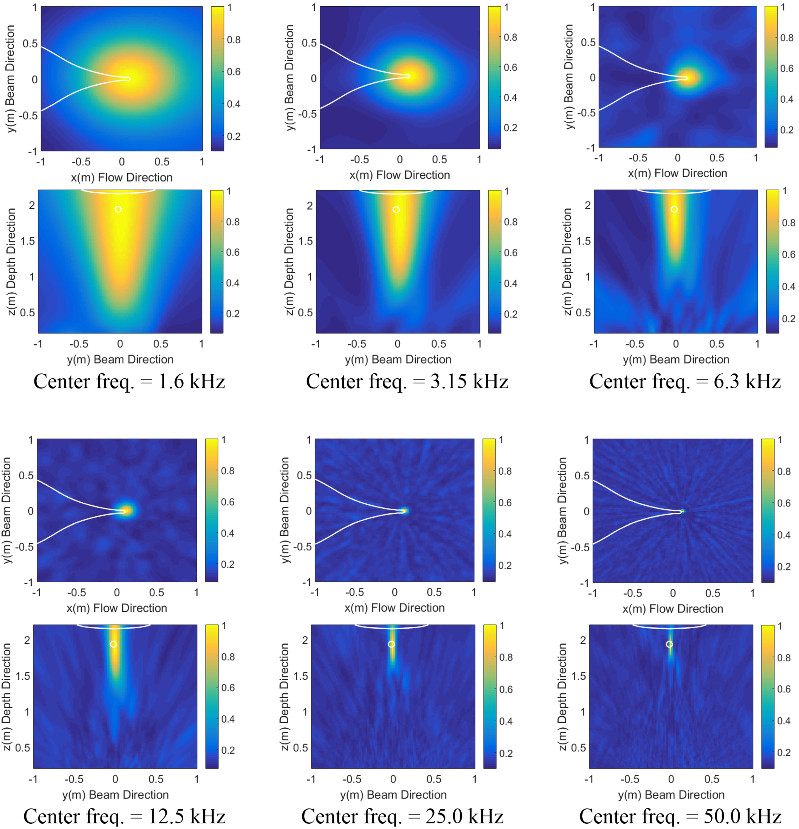
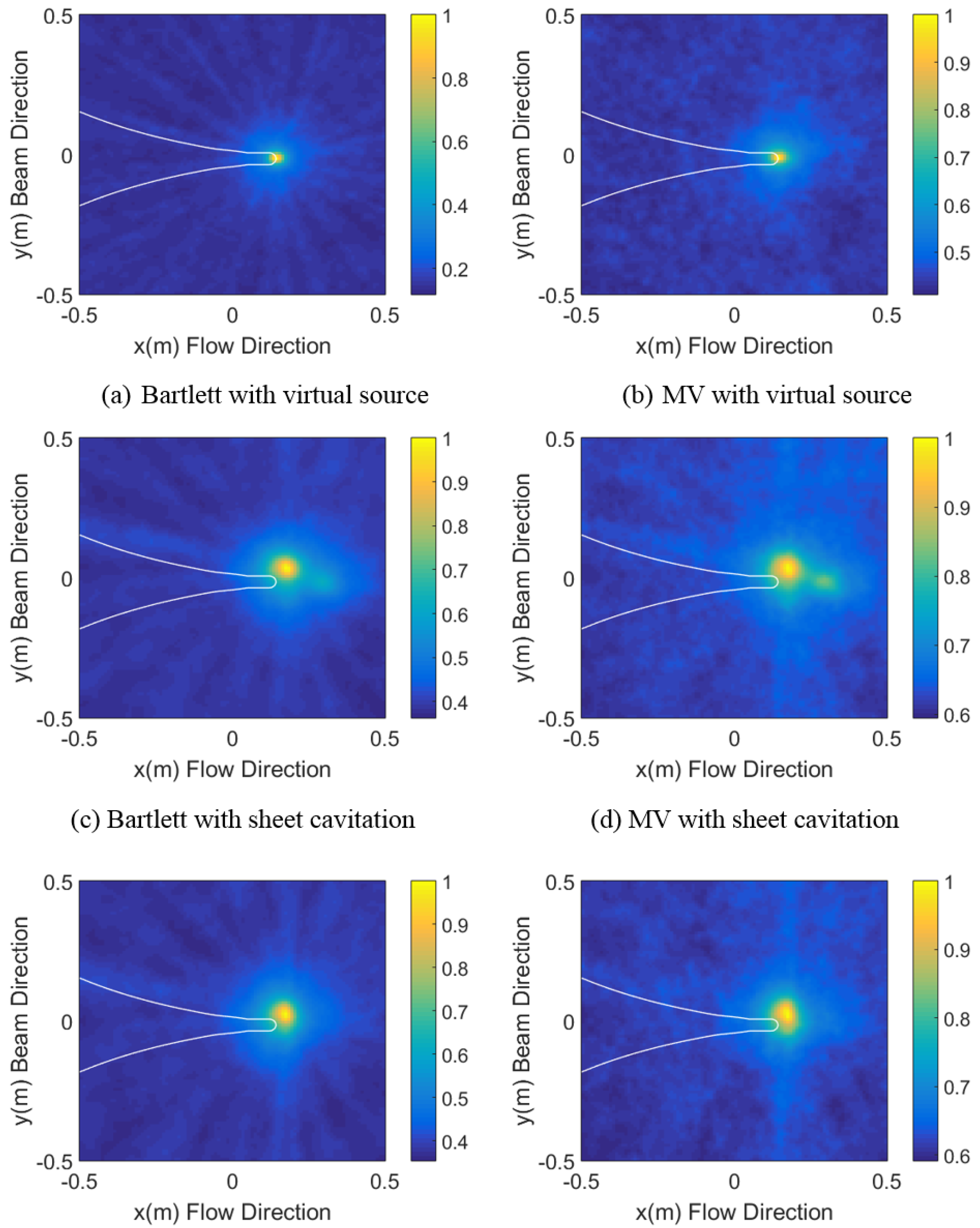
3.1. Virtual Source Experiment

An experiment was carried out using a virtual source installed at the end of the propeller shaft, as shown in Figure 6a. The ITC-1032 hydrophone was used as the virtual source, and it emitted white noise. The sound pressure level (SPL), which is averaged using the results from the 45 channels, is shown in Figure 6b. Green’s functions measured at the 45 hydrophones shown in Figure 4a are obtained by cross-correlating the input signal with the measured signals.
The measured noise data were digitized with the sn Equations (7) and (8). The frequency range is from 1 kHz to 100 kHz with a bandwidth resolution ( Δ f ) of 1 kHz. Figure 7 present the localization results using the objective function of Equations (7) and (8) for two different replica fields, i.e., Equations (5) and (6): (a) Bartlett processor + multiple arrivals; (b) MV processor + multiple arrivals; (c) Bartlett processor + direct arrival; (d) MV processor + direct arrivampling frequency ( f s ) of 240 kHz. We process them by employing the objective functions ial. Each plot in Figure 7 is composed of three orthogonal slices along the flow, beam and depth directions, which are also designated as the x-, y- and z-directions, respectively. Each slice, which is called an ambiguity surface, represents the normalized power of the values calculated from the objective function, such that the maximum value equals one. The high valued regions in each plot indicate the possible source locations. The outline of the model ship, which is cut vertically along the propeller shaft, is also shown in the plots.
From Figure 7, one distinct noise source is observed without ambiguity. The maximum processor power occurs at r s = (0.11 m, −0.02 m, 1.94 m), (0.11 m, −0.02 m, 1.90 m), (0.11 m, −0.02 m, 1.92 m) and (0.11 m, −0.02 m, 1.90 m) for the case of (a), (b), (c) and (d), respectively. The localization results for all cases are exactly the same, except for the source depth. It is observed that the replica with direct arrivals shows similar performance to that of multiple arrivals, implying that the direct arrival plays a dominant role in the localizations. It is also encouraging that the MV processor successfully localizes the virtual source, although the environment for the replica field might be different from the true one. The spatial resolution can be inferred from the main lobe contour in the ambiguity surface. From the ambiguity surface of the x-z plane (or y-z plane), vertically-elongated contour shapes are observed for all cases, which implies the poorer vertical resolution compared to the horizontal. This is due to the source-array configuration (see Figure 2), as discussed previously in Figure 5. The relatively large discrepancy between the estimated source depths can be explained by this, as well.
In order to investigate the array performance with respect to the frequency, one-third octave band analysis is performed. The direct arrivals are used as the replica in the processing. In each frequency band, the same number of data is used, and thus, the bandwidth resolution ( Δ f ) varies depending on the center frequency ( f c ) . The number of data is 30, and Δ f is 48 Hz, 97 Hz, 186 Hz, 379 Hz, 793 Hz and 1552 Hz for f c of 1.6 kHz, 3.15 kHz, 6.3 kHz, 12.5 kHz, 25 kHz and 50 kHz, respectively.
Figure 8 shows two orthogonal ambiguity surfaces (x-y and y-z planes) of the Bartlett processor for the one-third octave bands, of which the center frequency is as given in the plot. Figure 9 is for the MV processor. Each plane is cut to include the position of the maximum processor power, which is given in Table 1. As was stated in the previous Subsection 2.2, the phase sensitivity and, thus, the spatial resolution become high as the frequency increases. This frequency dependency is observed from the main lobes’ contour in the ambiguity surfaces. In addition, the directional dependency of the spatial resolution, which is mentioned above, is also commonly observed at all frequency bands. Table 1 shows the estimated source position for each frequency band. The mean position along with the standard deviation (SD) are also given. The mean source position agrees well with the previous estimates, (0.11 m, −0.02 m, 1.92 m) and (0.11 m, −0.02 m, 1.90 m) for the Bartlett and the MV processor, respectively. The source depth shows the maximum SD in both frequency. However, the error is still small compared to the diameter of ITC-1032 (6.86 cm) [36].

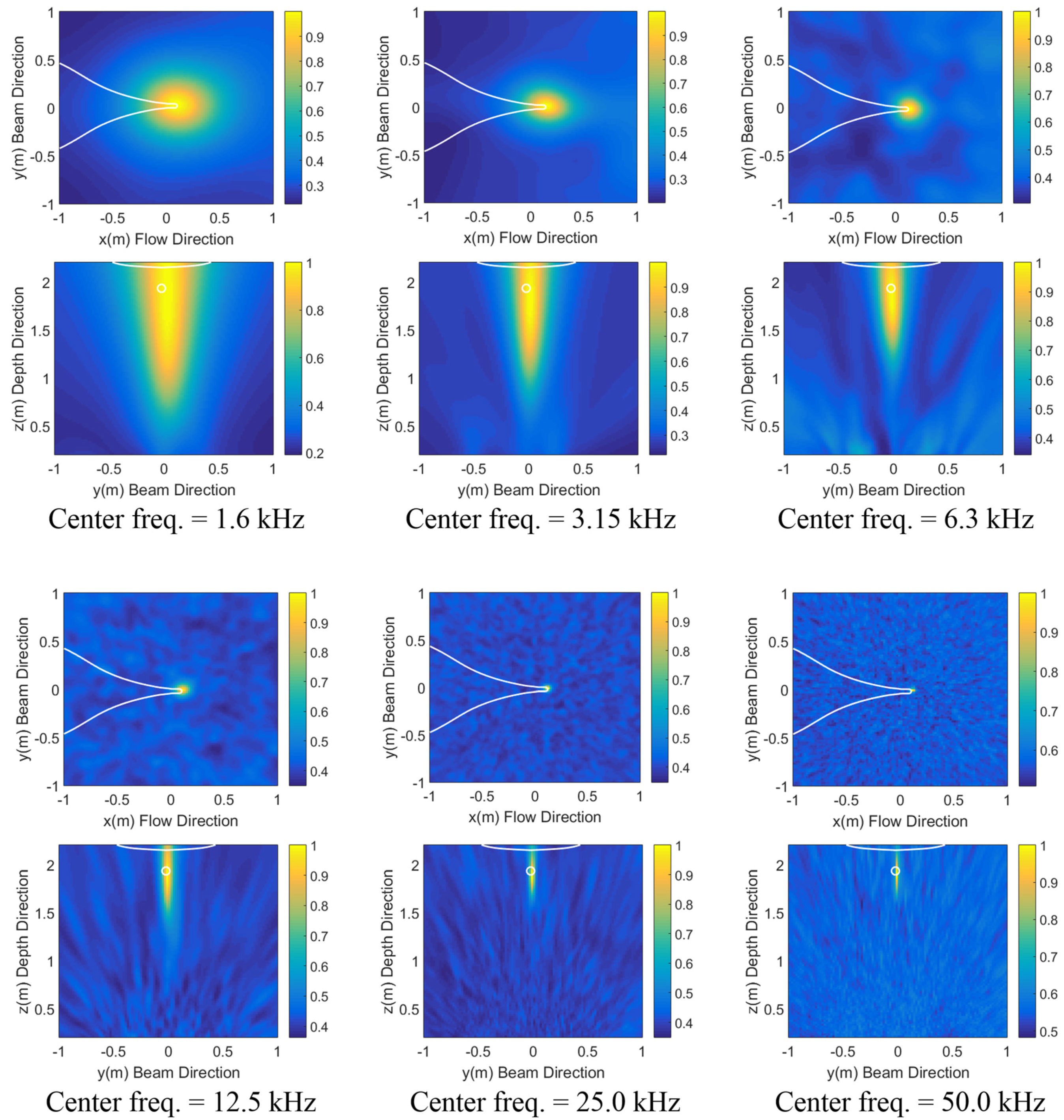
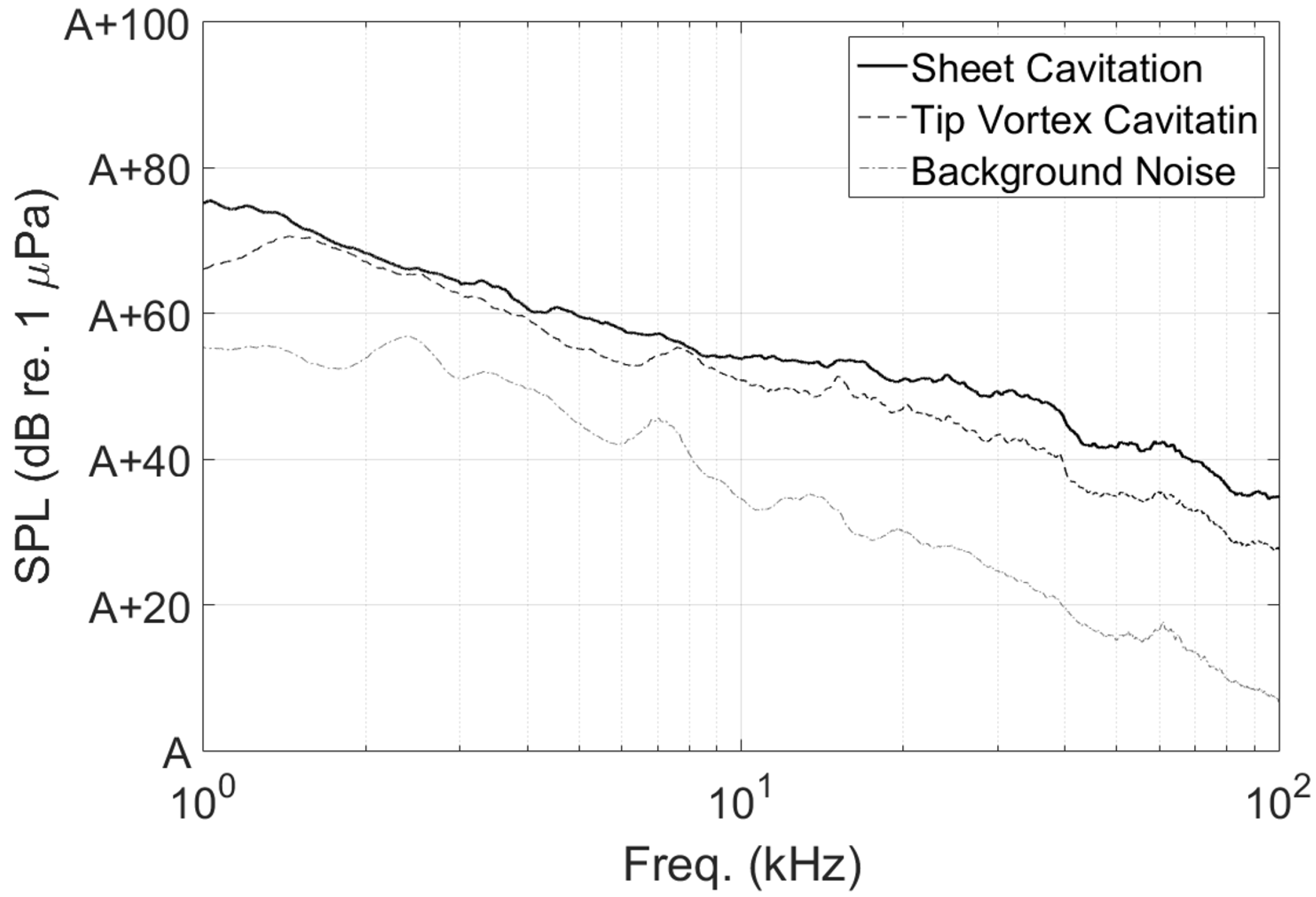
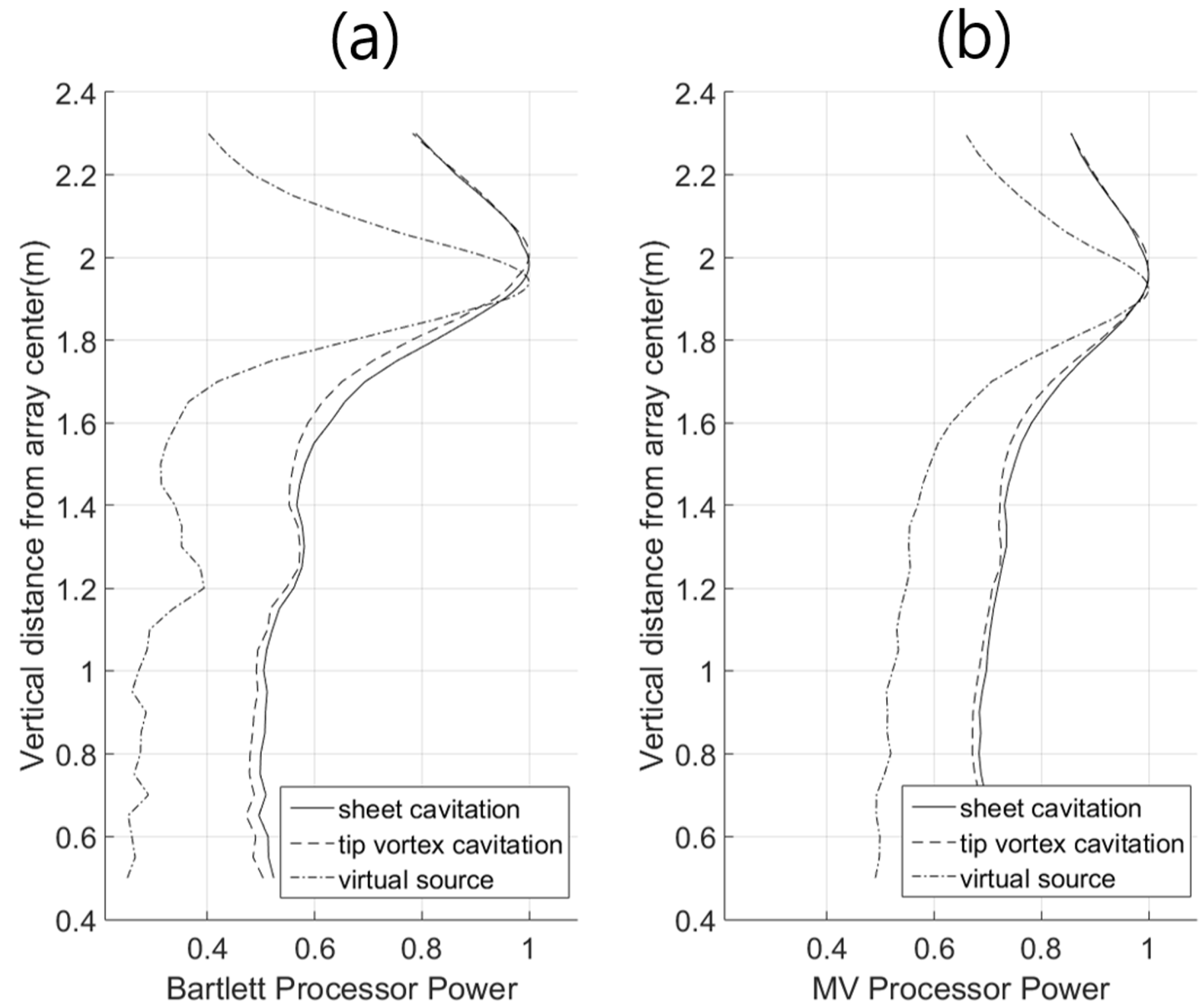
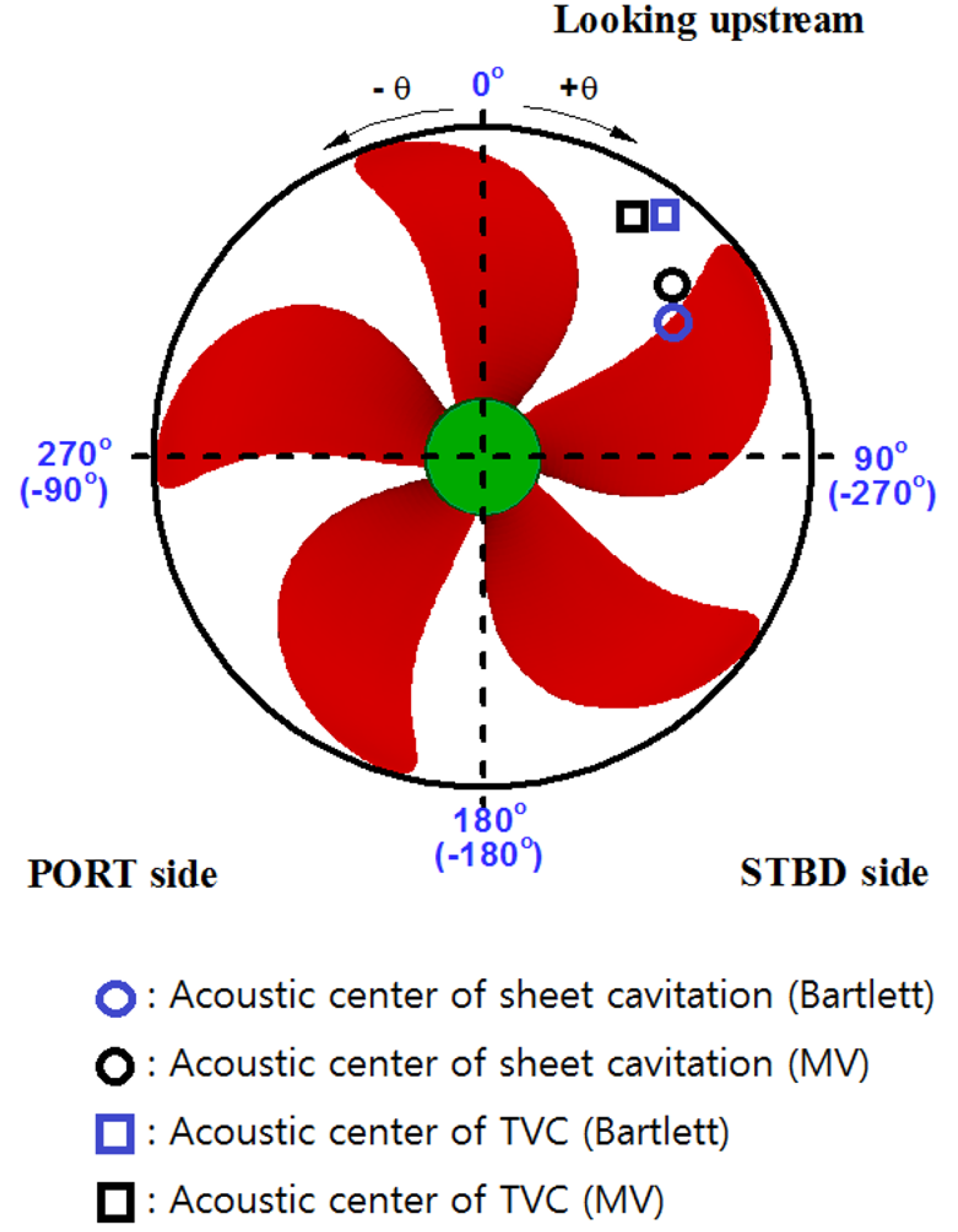
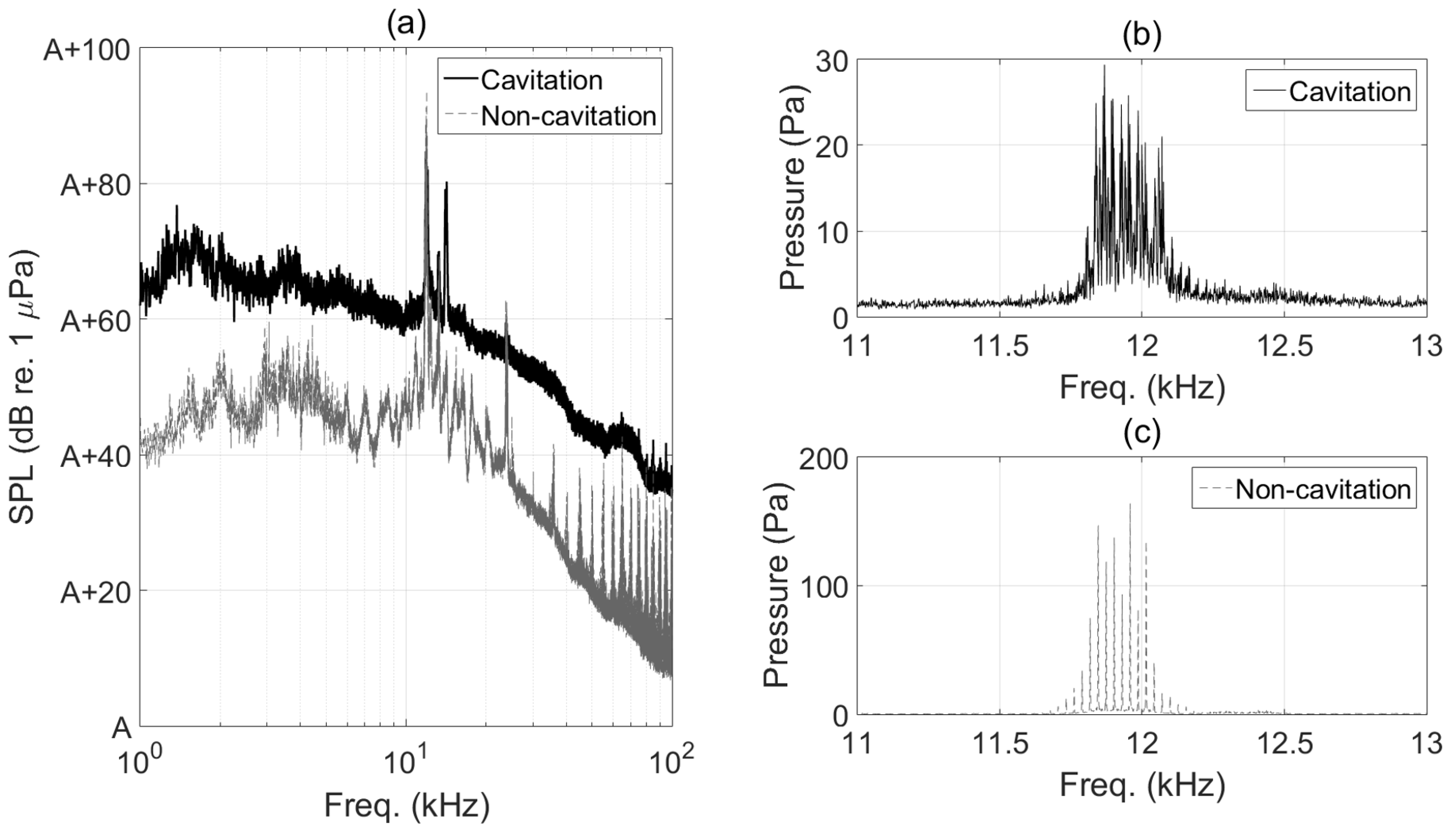
3.2. Propeller Cavitation Noise Experiment

Propeller cavitation experiments were performed for two test conditions. The first test condition was the operational condition of the ship at the load condition of the design draft, where sheet and tip vortex cavitations were observed at the same time. The propeller noise, which we name “sheet cavitation”, was measured during the cavitation observation test. In the second test, we adjusted the tunnel pressure in order to suppress the sheet cavitation and for the tip vortex to be prominent. The propeller noise, which we name “tip vortex cavitation”, was also measured. The background noise at two different conditions was measured after removing the propeller. Finally, the virtual source experiment was carried out in order to determine the reference position.
Figure 10 shows the average sound pressure levels of the 45-channel measurements for two cavitation noises. The SPL of the background noise for the test condition of sheet cavitation is also shown in the figure. The background noise for the tip vortex condition, which is not shown in the figure, was similar to that of sheet cavitation. From the figure, it is clear that the cavitation noise is much louder than the background noise for all frequency ranges. It is also noticeable that the sound pressure level of the sheet and tip vortex cavitations is higher than that of the tip vortex, and their difference increases from 9 kHz to about 30 kHz, then it seems to get practically constant up to 100 kHz.
In order to localize noise sources, the Bartlett processor (see Equation (7)), using the replica field of direct arrivals, was applied to a set of data with the frequency range from 5 kHz to 100 kHz, where Δ f is 1 kHz. The MV processor powers (see Equation (8)) were also calculated using the same data. The candidate source positions range from −0.5 m to 0.5 m in the flow and beam directions and from 0.5 m to 2.3 m in the depth direction, based on the reference point coinciding with the array center.
Figure 11 shows the maximum processor powers with respect to the depth for the virtual source, the sheet cavitation and the tip vortex cavitation. The values are normalized in order to achieve a maximum power of one. Figure 12 shows the ambiguity surfaces (x-y plane) corresponding to the depths where the maximum processor powers are obtained in Figure 11. The outline of the model ship, which is cut horizontally along the propeller shaft, is also shown in the plots. The positions of the maximum processor powers, which correspond to the estimated source positions, can be determined from Figure 11 and Figure 12, and the results are given in Table 2. Since the cavitation is spatially distributed, the estimated source position should be considered as the acoustic center of distributed noise sources.
The rotational direction of the propeller is right handed, and the angular position of a key blade is measured from the vertically upward position (0°) in a clockwise direction when the propeller is looked upstream. The notation of the angular position of the blade is shown in Figure 13. When the virtual source position is assumed to coincide with the propeller center, the acoustic centers of the sheet cavitation and the tip vortex cavitation can be calculated from the localization results.
According to the Bartlett localization results in Table 2, the acoustic centers of the sheet cavitation and the tip vortex cavitation are located at the radius of 0.72 R with the angle of 39.8° and at the radius of 0.82 R with the angle of 26.6°, respectively. In addition, the MV localizations showed maximum powers at the radius of 0.65 R with the angle of 45.0° for the sheet cavitation and at the radius of 0.86 R with the angle of 32.0° for the tip vortex cavitation. The acoustic centers for the sheet cavitation and the tip vortex cavitation are also shown in Figure 13.
Figure 14 shows photographs of the propeller sheet cavitation at the blade angles from 20° to 50°. The extent of the sheet cavitation seems to be at maximum at the angle of around 40° where the cavitation covers the blade above 0.7 R . The visual observation of the sheet cavitation agrees well with the acoustic centers estimated using the localization methods.

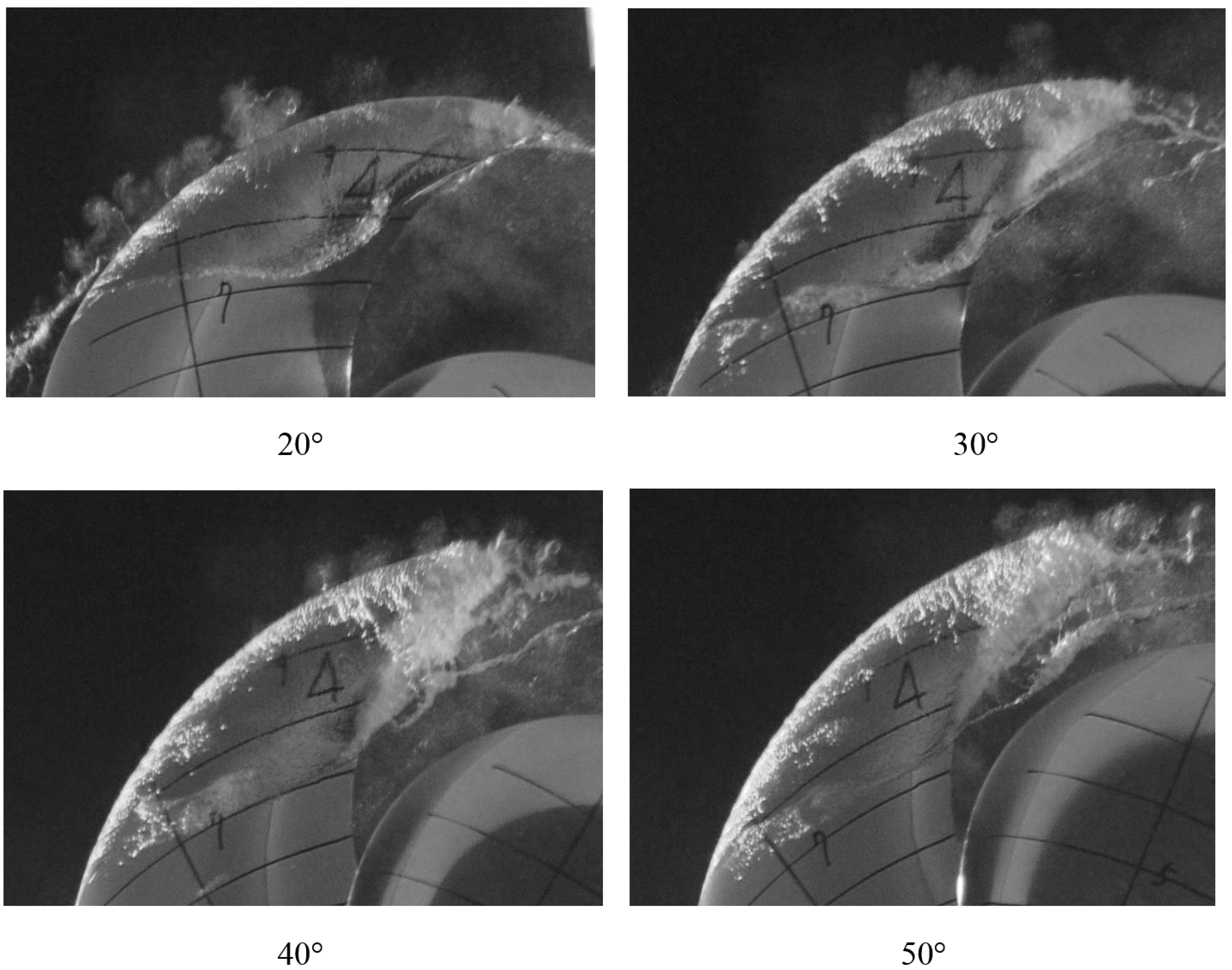
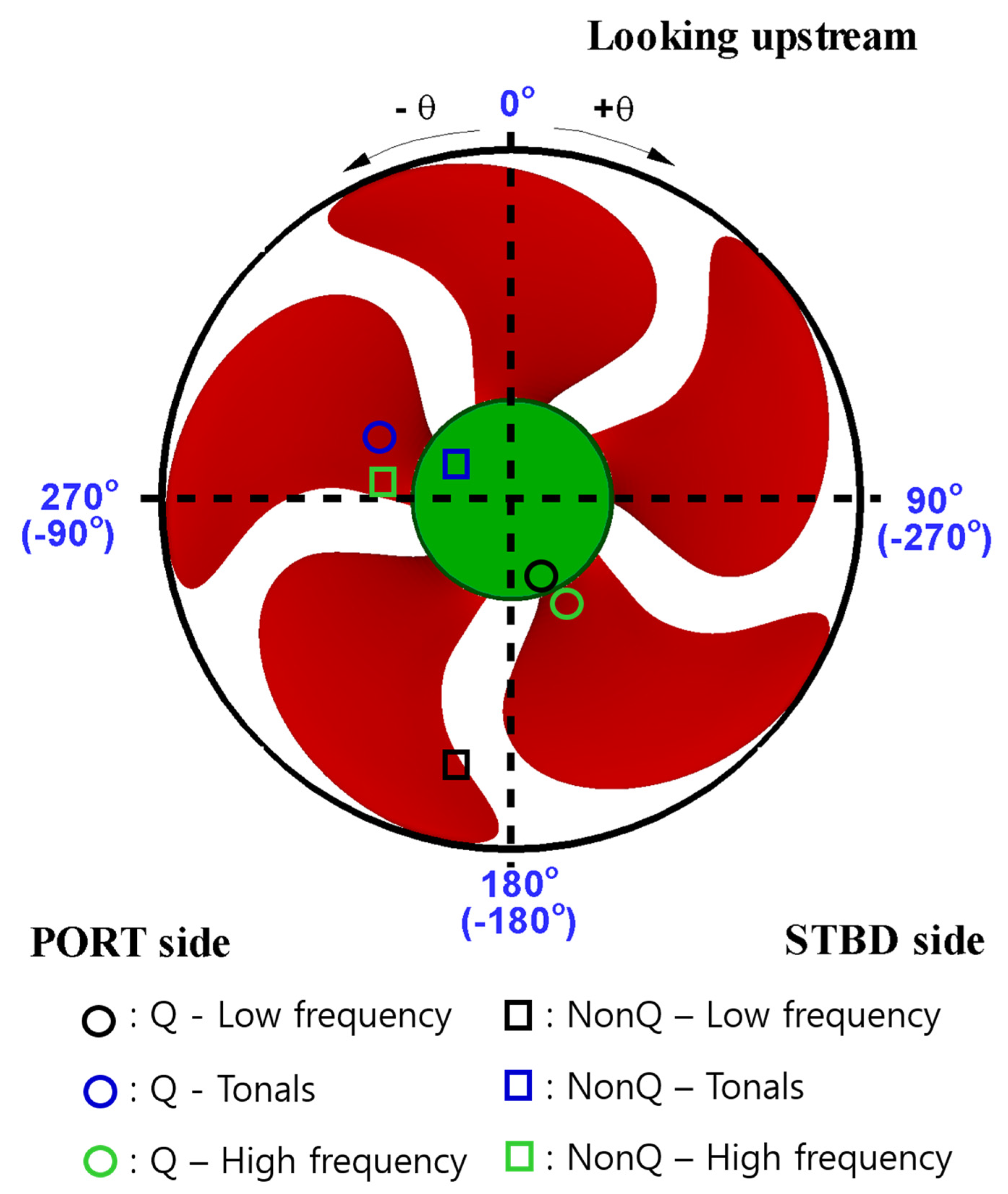
3.3. Propeller Singing Experiment

A cavitation test was carried out for the ship with twin propellers. The objective of the model test was to investigate the cavitation characteristics of the design propellers.
Figure 15a shows the average sound pressure levels of the 45-channel measurements for the cavitation noise and for the non-cavitation noise. The non-cavitation noise refers to the noise that was measured when no cavitation phenomenon was observed on the blade surfaces and around the propellers. In general, the sound pressure level of the non-cavitating propeller is much lower than that of the cavitating propeller. However, opposite results occurred for specific frequencies around 11 kHz. Figure 13c and Figure 15b show the frequency analysis results of both the cavitation noise and the non-cavitation noise, respectively, focusing on the frequency band of interest (11 to 13 kHz). From the figure, a train of high frequency tones is clearly seen for both cases. The difference frequency between two adjacent tones coincides with the propeller rotational speed. Thus, we were suspicious of the “propeller singing” [39].
In order to localize noise sources, the Bartlett processor (see Equation (7)) using the replica field of direct arrivals was applied to three sets of data: (i) the 5 to 0-kHz frequency range with Δ f of 100 Hz; (ii) tones in Figure 15; and (iii) the 20 to 30-kHz frequency range with Δ f of 500 Hz. The datasets are termed “low frequency data”, “tones” and “high frequency data”, respectively. The candidate source positions range from −0.5 m to 0.5 m in the flow and beam directions and from 0.5 m to 2.3 m in the depth direction.
Figure 16 shows the ambiguity surfaces (x-y plane) of cavitation and non-cavitation noise at the depths of maximum processor power. The estimated source positions, which correspond to the points yielding the maximum processer power, are given in Table 3. In the plots, the horizontal dashed line represents the keel line of the ship, and the vertical dashed-dotted line connects two propellers. The outline of the model ship, which is cut horizontally along the water line, is also shown in the plots.
With the low and high frequency data, two noise sources, which distinctly correspond to two propellers, are clearly localized for the non-cavitation noise, as well as for the cavitation noise. In contrast, a single noise source is present at the starboard side with the tonal localizations for both noise cases. However, this does not mean that a noise source does not exist at the port side. Applying the same localization method to only the port side region, we could also find a distinct noise source that is not given in the paper. The noise strength of the starboard side thus might be considered to overwhelm that of the port side, which implies that the starboard side propeller was singing during the noise measurement.
Figure 17 shows the estimated acoustic center of the starboard side propeller. From the figure, it is observed that noise sources are mostly scattered around the propeller hub, especially for the cavitation case. This result might reflect the complex cavitation behaviors, which are usual in the inclined twin-shafted propeller.

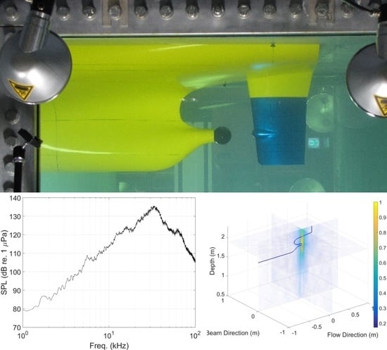
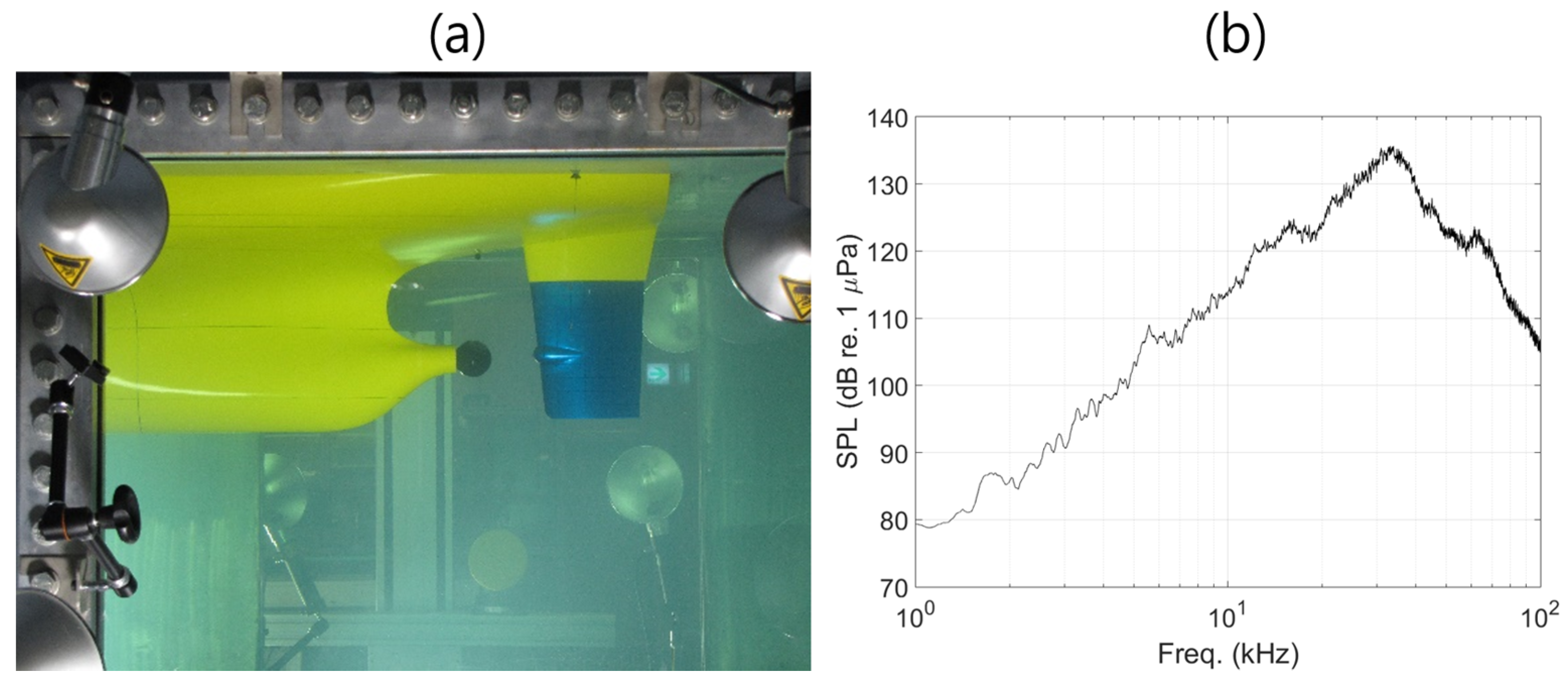
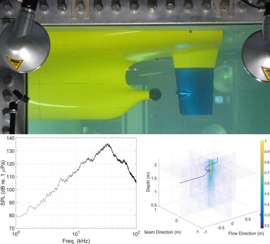
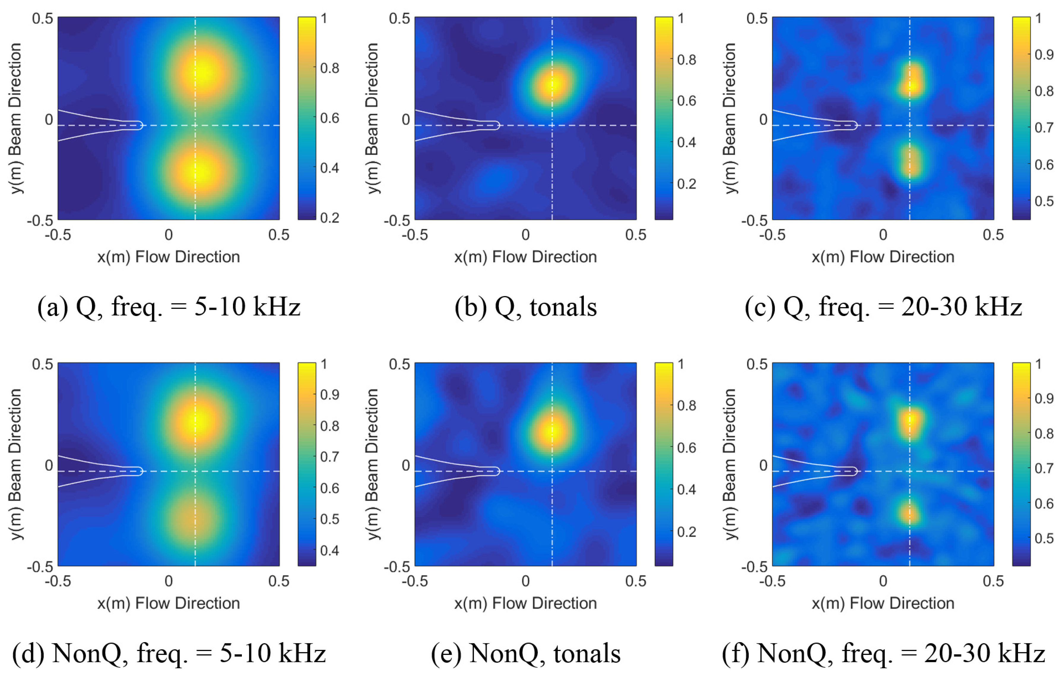
3.4. Underwater Vehicle Experiment

A cavitation test was carried out for the underwater vehicle in the large cavitation tunnel. The objective of the model test was to investigate the cavitation performance, including the cavitation inception speed of the designed propeller. The body of the vehicle was made of aluminum alloy according to the specified scale ratio between the model and the full ship. A driving motor and a dynamometer were installed inside the body. The background noise and the virtual source noise were also measured at the experiment, as well as the propeller noise.
Figure 18 shows the average sound pressure levels of the 45-channel measurements for the cavitation noise, the non-cavitation noise and the background noise. The test condition of background noise was the same as that of cavitation noise. From the figure, it is obvious that the cavitation noise is much louder than the background noise for all frequency ranges.
Figure 19 shows the ambiguity surfaces of various noise sources, such as the virtual source, propeller cavitation noise, non-cavitating propeller noise and background noise. The ambiguity surface of the x-y plane is obtained at the depth of maximum processor power, and that of the y–z plane is at the maximum processor range. The estimated source positions   ( x s ,   y s ,   z s ) , which correspond to the points yielding the maximum processer powers, are (−1.69 m, 0.03 m, 1.27 m) for the virtual source, (−1.68 m, −0.03 m, 1.37 m) for the cavitation noise, (−1.73 m, 0.03 m, 1.34 m) for the non-cavitation noise and (−2.40 m, 0.10 m, 1.33 m) for the background noise. In each plot, the white line represents the outline of the body, and the dashed circle is an imaginary disc of which the radius is the same as that of the propeller.
The model was installed for the propeller center to be 1.7 m upstream from the array center. Considering the estimated source positions, the model shifted to the end-fire region of the array (see Figure 2). Comparing the ambiguity surfaces in Figure 19 to the results in Figure 7 to Figure 9, the vertical resolution (z-direction) improves, and in contrast, the horizontal resolution (x-direction) deteriorates. The vertical variation of the phase difference between two receivers increases as the source approaches the end-fire region and then decreases again after a specific range, which is dependent on the source-receiver configuration, as shown in Figure 5d. The horizontal variation of phase difference between two receivers decreases monotonically as the source shifts from the broadside to the end-fire direction, as also shown in Figure 5d.
The localization results for the virtual source are given in Figure 19a,b as a reference. For the cavitation noise for which the localization results are shown in Figure 19c,d, the noise sources are distributed mainly in the upper part of the propeller, which agrees with the visual observation. The acoustic center of the non-cavitating propeller seems to exist at the blade surface approximately 0.4   R above the propeller center, as shown in Figure 19e,f.
Figure 19g,h shows the localization results for the background noise, which were measured by replacing the propeller with a dummy. In this case, the distributed noise sources are found inside the body, and the acoustic center coincides with the driving motor position. Thus, it is shown that the mechanical noise, as well as the propeller noise can be successfully localized by the proposed localization method using the array system.

4. Summary and Conclusions

The objective of the model test is to predict the noise level of the full ship and to control its noise signature. By localizing or identifying the noise source in model tests, it could be eliminated or its effect could at least be reduced at the design stage via applying a suitable noise measure, such as wake improvement, and/or the redesign of problematic objects, for example, a cavitating appendage. The noise localization method can also be used as a validation tool in the noise measurement by identifying whether there exists any other noise source than that of interest or not. Localizing noise sources in the model test might therefore be an important research subject along with measuring noise levels.
In this paper, we proposed a noise localization method using a 45-channel hydrophone array installed in the KRISO large cavitation tunnel. The noise measurement experiments were performed following the test procedure: (i) determining and setting of test condition, such as the propeller thrust coefficient K T and the cavitation number σ n ; (ii) measuring propeller noise; (iii) measuring background noise; and (iv) measuring the noise of the virtual source, if needed. For the localization method, two incoherent broadband processors, the Bartlett processor and the MV processor, are applied using simulated replica fields. The replica field can be constructed using multiple arrivals or only direct arrivals.
We carried out a noise experiment using a virtual source and scale models, including a ship with a single propeller, a ship with twin propellers and an underwater vehicle. Thus, the noise sources correspond to the virtual source, cavitating and non-cavitating propellers and the mechanical system, such as a driving motor. From the localization results, the following conclusions can be drawn.
(1)
The replica field constructed using direct arrivals shows reliable localization results. When the exact simulation of the tunnel environment is difficult, it is preferable to use the direct arrivals as the replica field.
(2)
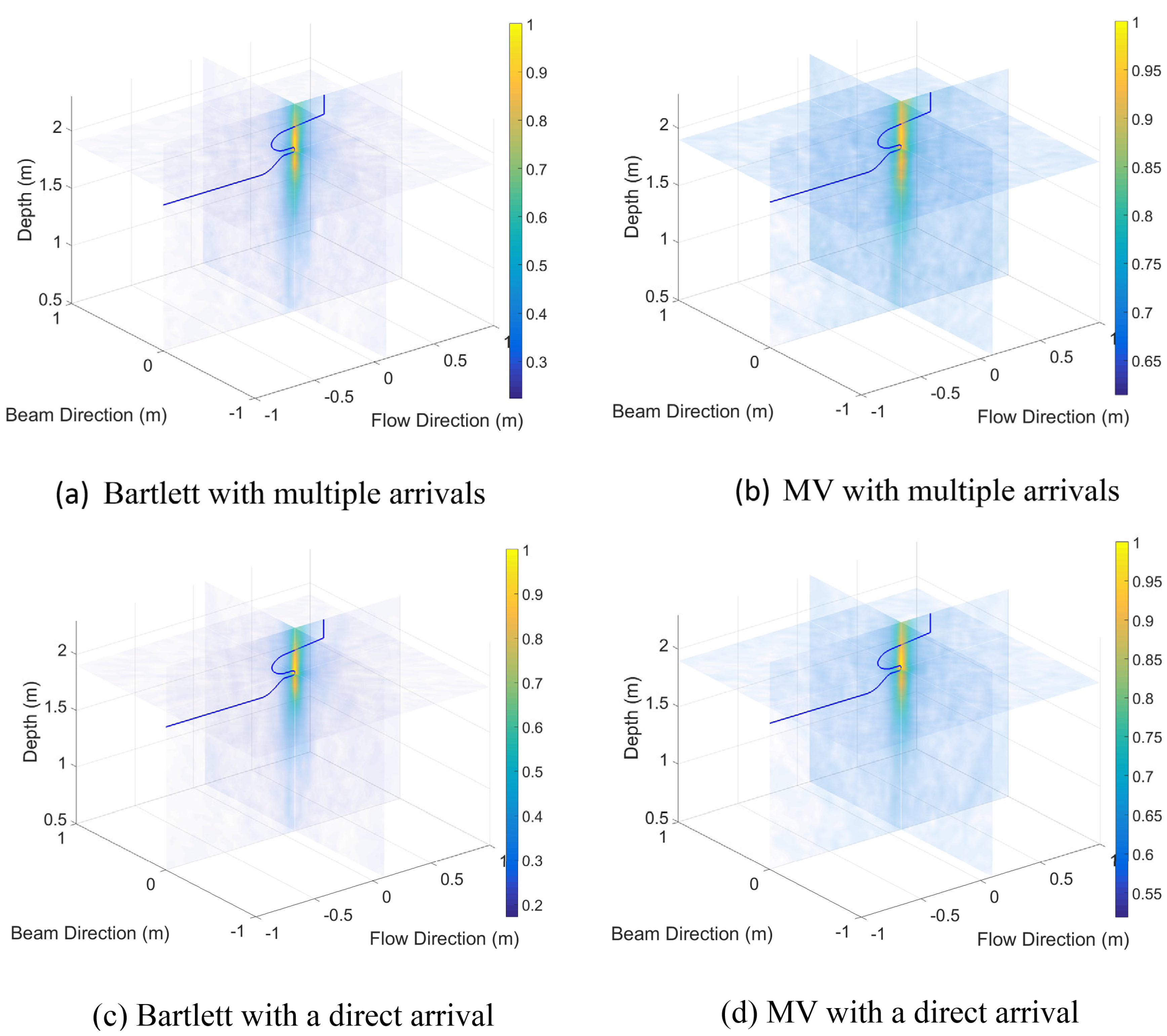
Both the Bartlett processor and the MV processor showed similar localization performances. However, the Bartlett processor seems to be more robust, especially when the sound pressure level is low.
(3)
The proposed localization method can be successfully applied to noise sources other than those of the propeller cavitation.
(4)
Finally, we suggest that the localization performance can be improved if the noise is measured at multiple array positions using a moving array system.

Acknowledgments

This work was supported by the Ministry of Trade, Industry and Energy (MOTIE) (project code: 10045337).

Author Contributions

All authors contributed equally to this work. Gun-Do Kim established the experimental plan and derived the test conditions for all experiments. Young-Ha Park was responsible for the experiments and data acquisition. Cheolsoo Park and Keunhwa Lee analyzed the measured data and derived the results. Woojae Seong initiated this work, reviewed the paper and discussed the results.

Conflicts of Interest

The authors declare no conflict of interest.

References

  1. Cavitation ITTC Committee. Final Report and Recommendations to the 15th ITTC. In Proceedings of the 15th ITTC, Hague, The Netherlands, 15–23 September 1978.
  2. Bark, G.; van Berlekom, W. Experimental investigations of cavitation noise. In Proceedings of the 12th Symposium on Naval Hydrodynamics, Washington, DC, USA, 9–14 August 1978.
  3. Latorre, R. Propeller tip vortex cavitation noise inception. In Proceedings of the SNAME Propellers’81 Symposium, Virginia Beach, VA, USA, 17–18 September 1981.
  4. Koop, B. Test Procedures for Hydro-Acoustic Investigations in the HSVA with Some Test Results; HSVA Report No. Ac 03/77; CORDIS: Hamburg, Germany, 1977. [Google Scholar]
  5. Thompson, D.E.; Billet, M.L. The Variation of Sheet Type surface Cavitation Noise with Cavitation Number; Applied Research Laboratory, Pennsylvania State University: Old Main, PA, USA, 1978. [Google Scholar]
  6. Bark, G.; Johnsson, C.A. Prediction of cavitation noise from model experiments in a large cavitation tunnel. In Noise Sources in Ships 1: Propellers; Nordforsk: Stockholm, Sweden, 1981. [Google Scholar]
  7. Blake, W.K.; Sevik, M.M. Recent developments in cavitation noise research. In Proceedings of the ASME International Symposium on Cavitation Noise, Phoenix, AZ, USA, 14–19 November 1982.
  8. Cavitation ITTC Committee. Final Report and Recommendations to the 18th ITTC. In Proceedings of the 18th ITTC, Kobe, Japan, 18–24 October 1987.
  9. Levkovskii, Y.L. Modelling of cavitation noise. J. Sov. Phys. Acoust. 1968, 13, 337–339. [Google Scholar]
  10. Lovik, A. Scaling of propeller cavitation noise. Noise Sources in Ships 1: Propellers; Nordforsk: Stockholm, Sweden, 1981. [Google Scholar]
  11. Strasberg, M. Propeller cavitation noise after 35 years of study. In Proceedings of the ASME International Symposium on Noise and Fluids Engineering, Atlanta, GA, USA, 16–20 June 1977.
  12. Blake, W.K. Acoustic measurements in cavitation testing. In Proceedings of the DRG Seminar on Advanced Hydrodynamic Testing Facilities, Hague, The Netherlands, 11–15 March 1982.
  13. Cavitation ITTC Committee. Final Report and Recommendations to the 16th ITTC. In Proceedings of the 16th ITTC, St. Petersburg, Russia, 27–30 June 1981.
  14. Ten Wolde, T.; De Bruijn, A. A new method for the measurements of the acoustical source strength of cavitating ship propellers. Int. Shipbuild. Progress 1975, 22, 385–396. [Google Scholar]
  15. Van der Kooji, J.; De Bruijn, A. Acoustic measurements in the NSMB depressurized towing tank. In Proceedings of the DRG Seminar on Advanced Hydrodynamic Testing Facilities, Hague, The Netherland; 1982. [Google Scholar]
  16. Noordzji, L.; Van der Kooji, J. Hydro-acoustics of a cavitating screw propeller; far-field approximation. J. Ship Res. 1981, 25, 90–94. [Google Scholar]
  17. Leggat, L.J. Propeller noise investigation in a free-field environment. In Proceedings of the DRG Seminar on Advanced Hydrodynamic Testing Facilities, Hague, The Netherlands, 26–28 April 1982.
  18. Abbot, P.A.; Celuzza, S.A.; Etter, R.J. The acoustic characteristics of the Naval Surface Warfare Center's Large Cavitation Channel (LCC). In Proceedings of the ASME Winter Annual Meeting, New Orleans, LA, USA, 28 November–3 December 1993.
  19. Friesch, J. The new cavitation test facility of Hamburg Ship Model Basin (HYKAT). In Proceedings of the International Symposium on Hydro- and Aerodynamics in Marine Engineering, Varna, Bulgaria, 28 October–1 November 1991.
  20. Sato, R.; Mori, T.; Yakushiji, R.; Naganuma, K.; Nishimura, M.; Nakagawa, K.; Sasajima, T. Conceptual design of the flow noise simulator. In Proceedings of the 4th ASME_JSME Joint Fluids Engineering Conference, Honolulu, HI, USA, 6–10 July 2003.
  21. Van Trees, H.L. Part IV of detection, estimation, and modulation theory. In Optimum Array Processing; John Wiley & Sons, Inc.: New York, NY, USA, 2002. [Google Scholar]
  22. Tolstoy, A. Matched Field Processing for Underwater Acoustics; World Scientific: Hackensack, NJ, USA, 1993. [Google Scholar]
  23. Baggeroer, A.B.; Kuperman, W.A.; Mikhalevsky, P.N. An overview of matched field methods in ocean acoustics. IEEE J. Ocean. Eng. 1993, 18, 401–424. [Google Scholar] [CrossRef]
  24. Muller, T.J. Aeroacoustic Measurements; Springer: Berlin, Germany, 2002. [Google Scholar]
  25. Park, C.; Seol, H.; Kim, K.; Seong, W. A study on propeller noise source localization in a cavitation tunnel. Ocean Eng. 2009, 46, 754–762. [Google Scholar] [CrossRef]
  26. Chang, N.A.; Dowling, D.R. Ray-based acoustic localization of cavitation in a highly reverberant environment. J. Acoust. Soc. Am. 2009, 125, 3088–3100. [Google Scholar] [CrossRef] [PubMed]
  27. Chang, N.A.; Ceccio, S.L. The acoustic emissions of cavitation bubbles in stretched vortices. J. Acoust. Soc. Am. 2011, 130, 3209–3219. [Google Scholar] [CrossRef] [PubMed]
  28. Anderson, S. Acoustic Cavitation Localization in Reverberant Environments. Master’s Thesis, The Pennsylvania State University, State College, PA, USA, 13 December 2012. [Google Scholar]
  29. Lee, K.; Lee, J.; Kim, D.; Kim, K.; Seong, W.; Lee, J. Propeller sheet cavitation noise source modeling. J. Sound Vib. 2014, 333, 1356–1368. [Google Scholar] [CrossRef]
  30. Kim, D.; Lee, K.; Seong, W. Non-cavitating propeller noise modeling and inversion. J. Sound Vib. 2014, 333, 6424–6437. [Google Scholar] [CrossRef]
  31. Kim, D.; Seong, W.; Choo, Y.; Lee, J. Localization of incipient tip vortex cavitation using ray based matched field inversion method. J. Sound Vib. 2015, 354, 34–46. [Google Scholar] [CrossRef]
  32. Felli, M.; Falchi, M.; Pereira, F. Investigation of the Flow Field around a Propeller-Rudder Configuration: On-Surface Pressure Measurements and Velocity-Pressure-Phase-Locked Correlations. In Proceedings of the Second International Symposium on Marine Propulsors, Hamburg, Germany, 17–18 June 2011.
  33. Brüel & Kjær. Hydrophones—Types 8103, 8104, 8105 and 8106. Available online: http://www.lthe.fr/LTHE/IMG/pdf/DocBruelKjaerHydro.pdf (accessed on 3 December 2015).
  34. Park, C.; Seol, H.; Kim, G.-D.; Park, Y.-H. A study on hydrophone array design optimization for cavitation tunnel noise measurement. J. Acoust. Soc. Korea 2013, 32, 237–246. [Google Scholar] [CrossRef]
  35. ITTC. Recommended Procedures and Guidelines 7.5-02-01-05: Model Scale Noise Measurements; ITTC: Centurion, South Africa, 2014. [Google Scholar]
  36. International Transducer Corporation. Deep Water Omnidirectional Transducer Model ITC-1032. Available online: http://www.channeltechgroup.com/publication/model-itc-1032-deep-water-omnidirectional-transducer/ (accessed on 3 December 2015).
  37. Tani, G.; Viviani, M.; Armelloni, E.; Nataletti, M. Cavitation Tunnel Acoustic Characterisation and Application to Model Propeller Radiated Noise Measurements at Different Functioning Conditions. Available online: http://pim.sagepub.com/content/early/2015/01/09/1475090214563860.abstract (accessed on 15 January 2015).
  38. Oppenheim, A.V.; Schafer, R.W. Discrete-Time Signal Processing; Prentice-Hall: Upper Saddle River, NJ, USA, 1989. [Google Scholar]
  39. Ross, D. Mechanics of Underwater Noise; Pergamon Press Inc.: New York, NY, USA, 1976. [Google Scholar]
Figure 1. Schematic diagram of the KRISO large cavitation tunnel.
Remotesensing 08 00195 g001
Figure 2. Forty five-channel hydrophone array configuration inside the acoustic trough.
Remotesensing 08 00195 g002
Figure 3. Beam patterns of the uniformly-weighted planar array at the frequencies of: (a) 2 kHz; (b) 4 kHz; (c) 8 kHz; and (d) 16 kHz. All of the beam patterns are calculated at the azimuth angle of 0°. The direction of arrival (DoA) refers to the elevation angle with the azimuth angle of 0°.
Remotesensing 08 00195 g003
Figure 4. Measured (a) and simulated (b) Green’s function for the 45-channel hydrophones. The schematic diagram of multiple reflections and the detail for bottom-reflected arrival are shown in (c). DBm, multiple reflections between the acoustic window and array plate.
Remotesensing 08 00195 g004
Figure 5. The definition of the half power beam width (HPBW) (a) and HPBWs simulated with respect to the source position at r s = ( x s ,   0.0   m , 1.3 m ) under the condition of 8 kHz and 0 dB SNR for the Bartlett processor (b) and for the minimum variance (MV) processor (c); The color bar in (a) represents the value of Φ ( r ^ s ) / Φ ( r s ) . The phase sensitivity simulated under the same condition is shown in (d); The receiver positions are assumed as (−0.1 m, 0 m, 0 m) and (0.1 m, 0 m, 0 m) in the phase sensitivity calculation.
Remotesensing 08 00195 g005
Figure 6. Configuration of the virtual source experiment (a) and measured sound pressure level (b), which is averaged for the 45-channel hydrophones. (SPL: sound pressure level, Freq.: frequency).
Remotesensing 08 00195 g006
Figure 7. Localization results of the virtual source experiment for the various combinations of replica fields and matched field processing (MFP) processors: (a) Bartlett processor with multiple arrival replica fields; (b) MV processor with multiple arrival replica fields; (c) Bartlett processor with direct arrival replica fields; and (d) MV processor with direct arrival replica fields. “Depth (m)” in the plots refers to the vertical distance from the array center. The outline of the model ship, which is cut vertically along the propeller shaft, is shown with blue lines. The color bar in each plot represents the normalized value as Φ ( r ^ s ) / max { Φ ( r ^ s ) } , such that the maximum equals one.
Remotesensing 08 00195 g007
Figure 8. Ambiguity surfaces of the Bartlett processor with direct arrivals using the 1/3 octave bands of which the center frequencies are shown in the plots. The reference position of the plane cut is r ^ s = (0.1 m, −0.02 m, 1.93 m). The outline of the model ship, which is cut correspondingly to each plane, is shown with the white line.
Remotesensing 08 00195 g008
Figure 9. Ambiguity surfaces of the MV processor with direct arrivals using the 1/3 octave bands of which the center frequencies are shown in the plots. The reference position of the plane cut is r ^ s = (0.1 m, −0.02 m, 1.93 m). The outline of the model ship, which is cut correspondingly to each plane, is shown with the white line.
Remotesensing 08 00195 g009
Figure 10. Sound pressure levels of the sheet cavitation, the tip vortex cavitation and the background noise. (A: a reference value).
Remotesensing 08 00195 g010
Figure 11. Maximum powers of the Bartlett processor (a) and the MV processor (b) with respect to depth for the virtual source, the sheet cavitation and the tip vortex cavitation.
Remotesensing 08 00195 g011
Figure 12. Ambiguity surfaces (x-y plane) corresponding to the depths where the maximum processor powers are obtained in Figure 11. The outline of the model ship, which is cut horizontally along the propeller shaft, is shown with white lines.
Remotesensing 08 00195 g012
Figure 13. Notation of the blade angular position for the right-handed propeller when looking upstream. The estimated acoustic centers are also shown as circles (O) for the sheet cavitation and as squares (□) for the tip vortex cavitation. (TVC: tip vortex cavitation, STBD: starboard).
Remotesensing 08 00195 g013
Figure 14. Photographs of the propeller sheet cavitations at the blade angles from 20° to 50°.
Remotesensing 08 00195 g014
Figure 15. Average sound pressure levels of the 45-channel measurements for the cavitation noise and for the non-cavitation noise (a); tonal components for the cavitation noise (b); and the non-cavitation noise (c).
Remotesensing 08 00195 g015
Figure 16. Ambiguity surfaces (x-y plane) of cavitation (ac) and non-cavitation noise (df) at the depths of maximum processor power in Table 3. “Q” refers to the cavitation and “NonQ” refers to the non-cavitation. The horizontal dashed line represents the keel line of the ship, and the vertical dashed-dotted line connects two propellers. The outline of the model ship, which is cut horizontally along the water line, is also shown with white lines.
Remotesensing 08 00195 g016
Figure 17. The estimated acoustic centers for the cavitation noise (O) and for the non-cavitation noise (□). The frequency conditions are as given in the plot.
Remotesensing 08 00195 g017
Figure 18. Average sound pressure levels of the 45-channel measurements for the cavitation noise, the non-cavitation noise and the background noise.
Remotesensing 08 00195 g018
Figure 19. Ambiguity surfaces (x-y plane and y-z plane) of the virtual source (a,b); propeller cavitation noise (c,d); non-cavitating propeller noise (e,f) and background noise (g,h); at the depth and the range of the maximum processor power. In each plot, the white line represents the outline of the body, and the dashed circle is an imaginary disc of which the radius is the same as the propeller.
Remotesensing 08 00195 g019
Table 1. Estimated noise source positions ( x s ,   y s ,   z s ) for the virtual source experiment.
Center FrequencyBartlett ProcessorMV Processor
1.6 kHz(0.10 m, 0.0 m, 1.94 m)(0.09 m, 0.02 m, 1.92 m)
3.15 kHz(0.11 m, 0.01 m, 1.85 m)(0.14 m, 0.0 m, 1.86 m)
6.3 kHz(0.11 m, −0.02 m, 1.88 m)(0.12 m, −0.03 m, 1.88 m)
12.5 kHz(0.10 m, −0.02 m, 1.92 m)(0.11 m, −0.02 m, 1.87 m)
25.0 kHz(0.11 m, −0.02 m, 1.91 m)(0.11 m, −0.02 m, 1.89 m)
50.0 kHz(0.11 m, −0.02 m, 1.91 m)(0.11 m, −0.02 m, 1.91 m)
Mean(0.11 m, −0.01 m, 1.90 m)(0.11 m, −0.01 m, 1.89 m)
SD(0.01 m, 0.01 m, 0.03 m)(0.01 m, 0.01 m, 0.02 m)
Table 2. Estimated noise source positions ( x s ,   y s ,   z s ) for the propeller cavitation noise experiment.
Bartlett ProcessorMV Processor
Virtual Source(0.14 m, −0.02 m, 1.93 m)(0.14 m, −0.02 m, 1.92 m)
Sheet Cavitation(0.17 m, 0.03 m, 1.99 m)(0.17 m, 0.03 m, 1.97 m)
Tip Vortex Cavitation(0.17 m, 0.02 m, 2.01 m)(0.17 m, 0.02 m, 2.00 m)
Table 3. Estimated noise source positions ( x s ,   y s ,   z s ) for the propeller singing noise experiment.
TypeLow Frequency Data (5 to 10 kHz)TonesHigh Frequency Data (20 to 50 kHz)
Cavitation(0.15 m, 0.22 m, 1.85 m)(0.12 m, 0.16 m, 1.91 m)(0.13 m, 0.23 m, 1.84 m)
Non-cavitation(0.14 m, 0.19 m, 1.78 m)(0.11 m, 0.19 m, 1.90 m)(0.11 m, 0.16 m, 1.89 m)

