Spectral Characteristics of Common Reed Beds: Studies on Spatial and Temporal Variability

Abstract

Reed beds are the second largest producer of biomass in Olkiluoto Island. Quantitative information on the extent and amount of reed stands is an integral part of the biosphere assessment related to long-term safety analysis of nuclear fuel repository site currently under construction. The major challenge in reed bed mapping is discrimination between reed and other green vegetation. Spectral field measurements were used to study the temporal and spatial variability of spectral characteristics of reed beds. Feasibility of discriminating reed beds from other vegetation based on hyperspectral measurements was studied as well. Results indicate that there is large temporal variation of reed bed spectra and the optimal time for data acquisition differs for old and new reed bed types. Comparing spectral characteristics of the reed bed and meadow classes in a local neighborhood indicated that the classes have high within-class spectral variability and similar mean spectra, however, 10 out of 11 targets had lower angle to the mean spectrum of the corresponding class than that of the other class when Spectral Angle Mapper (SAM) was used. Comparing the spectral characteristics of reed beds at four test sites within the Olkiluoto Island indicated that while some of the sites had similar spectra, the difference between others was remarkable. This is partly explained by different density and height of dead and live reed stems at the four sites.

1. Introduction

Common reed (Phragmites Australis), a native helophyte in coastal areas of the Baltic Sea, has significantly spread on the Finnish coast during the last decades raising ecological issues and concerns due to the important role it plays in the ecosystem dynamics of shallow coastal areas [1]. In addition to biodiversity there are other ecological and economic issues such as water protection, bioenergy, construction, farming and landscape. Reed beds have proven to be effective in the treatment of waste waters such as domestic sewage and industrial discharge containing heavy metal wastes [2]. Reed biomass can be used as an energy source in three ways, namely by combustion, biogas production and biofuel production [3]. There are currently studies aiming to develop economical and sustainable methods to harvest reed for bioenergy production in Finland. Reed can be used as a soil conditioner in agriculture thus substituting the use of fertilizers [4].

Recent developments in sensor technology and data processing methods have led to an increase in the use hyperspectral imagery for environmental applications. High spectral and spatial resolution imagery provides researchers the potential to map vegetation at species’ level, provided the plant species under study are spectrally distinct [5]. Species discrimination using remote sensing is based on the assumption that each species is characterized by a set of unique biophysical features and biochemical composition that control the variability in its spectral signature [6].

The fundamental problem in vegetation discrimination using remote sensing is that there is an overall qualitative similarity in the spectral reflectance of green plant species. Furthermore, the assumption that individual plant species have unique spectral signatures may be wrong. Price [7] has argued that several species may actually have quantitatively similar spectra due to the spectral signature variation present within a species.

The capability of discriminating plant species using hyperspectral imagery has been demonstrated in many studies. Clark et al. [8] successfully discriminated tropical rain forest tree species. Schmidt and Skidmore [9] studied the discrimination of vegetation types in coastal wetlands. Thenkabail [10] used hyperspectral data to discriminate agricultural crops. Vahtmäe et al. [11] demonstrated the feasibility of hyperspectral remote sensing for mapping benthic microalgae cover. The remote sensing of wetlands does, to some extent, differ from remote sensing based mapping of other terrestrial features. Differences exist because wetlands occupy a unique interface between aquatic and terrestrial ecosystems [12]. In addition, the reflectance spectra of wetland vegetation canopies are often very similar and are combined with reflectance spectra of underlying soil [13]. The frequent and rapid changes of water depth and salinity add to the complexity of analyzing wetland environment using remote sensing.

The use of remote sensing in reed bed discrimination has been studied in several publications. Pengra et al. [14] evaluated the use of the spaceborne Hyperion sensor. The classification of reed beds showed good overall accuracy of 81.4%. It was found, however, that the small size and spatial arrangement of Phragmites stands was less than optimal considering Hyperion’s spatial resolution of 30 m. Lopez et al. [15] studied the discrimination of Phragmites using airborne hyperspectral data collected by the Probe-1 sensor. The study produced Phragmites maps showing an estimated accuracy of 80%. Onojeghuo and Blackburn [16] proposed the use of airborne hyperspectral and LiDAR data in reed bed discrimination. A comprehensive set of methods such as Principal Component Analysis (PCA), Spectrally Segmented PCA (SSPCA) and Minimum Noise Fraction (MNF) were applied to the hyperspectral data and combined with LiDAR derived measures including those based on texture analysis. A significant improvement (+11%) in the accuracy of reed bed delineation was achieved when a LiDAR-derived Canopy Height Map (CHM) was used together with the optimal SSPCA data set. Stratoulias et al. [17] used airborne AISA Eagle data in order to derive narrow band spectral indices used to characterize reed beds’ ecological status. Seasonal time-series studies can provide important information on spectral variability. Given the dynamic character of vegetation cover, a snapshot in time is not nearly as revealing as a time sequence [18]. Ouyang et al. [19] studied the spectral characteristics of Phragmites and two other wetland species using time-series analysis. The results showed that differences among saltmarsh communities’ spectral characteristics were affected by their phenological stages. Artigas and Yang [20] published a field-collected seasonal time-series of Phragmites spectra. The measured spectra were used to determine the vigor gradient of plants in marshlands.

Several measures have been proposed to quantify spectral similarity or separability of targets [21], Euclidean Distance (ED) being probably the most well-known measure used. Spectral Angle Mapper (SAM) is another well-established similarity measure in remote sensing applications. SAM is related to Pearson’s Correlation Coefficient, sometimes also called Spectral Correlation Mapper (SCM) in remote sensing literature. An advantage of Pearson’s Correlation Coefficient over SAM is its ability to distinguish between negative and positive correlation. Spectral Information Divergence (SID) classifier represents an information theoretic approach to hyperspectral classification. SID compares the similarity between two spectra by measuring the probabilistic discrepancy between two corresponding spectral signatures. In principle, the similarity between two spectra has two components: similarity in absolute level of reflectance and similarity in spectral shape. In this study, both of these components of similarity are assessed using the Euclidean Distance and Spectral Angle measures. Jeffries–Matusita distance (JM) was used as a statistical separability measure.

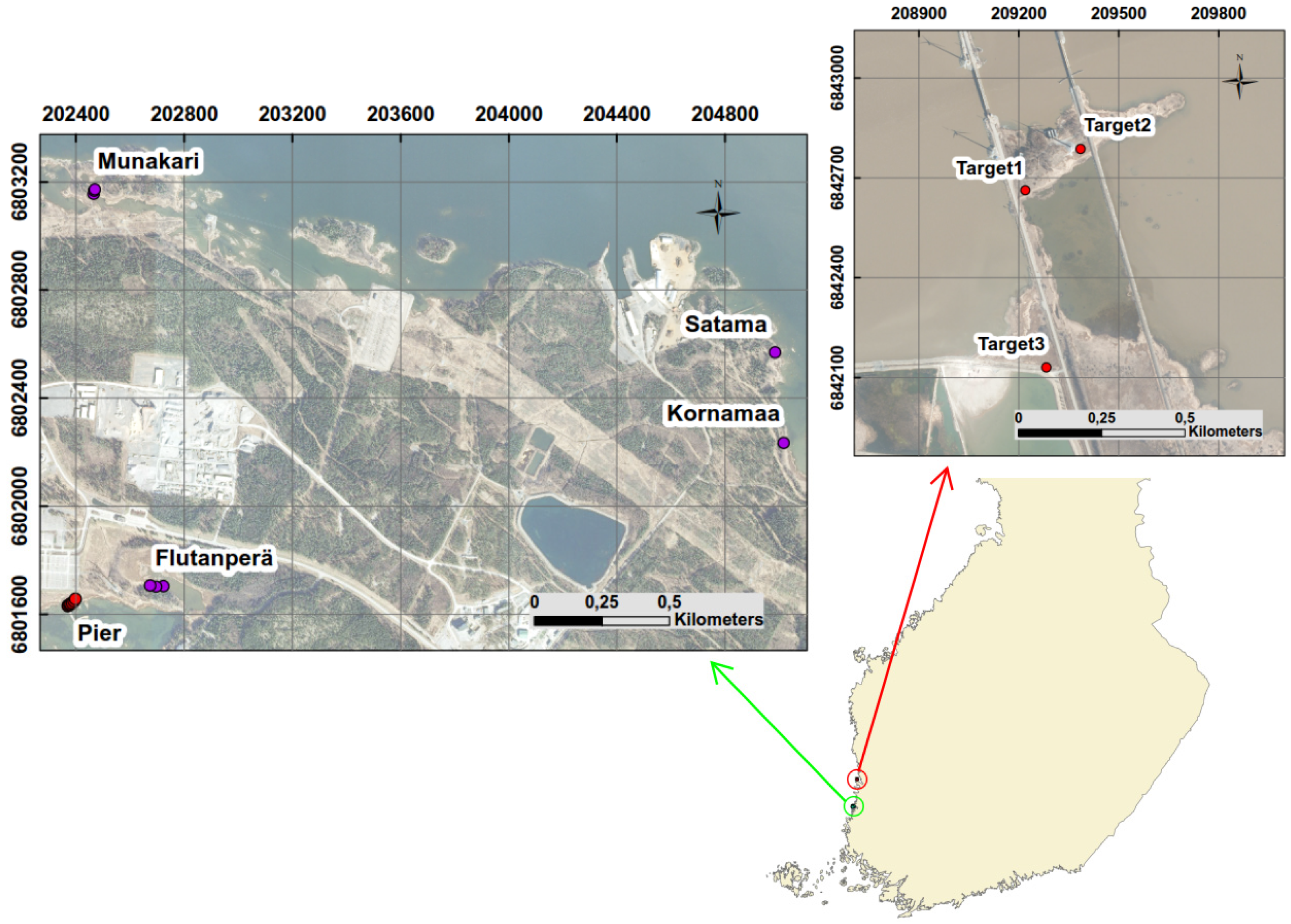
Reed beds cover significant part of the shoreline of the Olkiluoto Island. Reed can be found on gyttja, clay, till or stone bottoms [22]. The extent and vitality of the reed beds varies significantly, depending on the soil type and degree of shelter [22]. A repository site for spent nuclear fuel is currently under construction in Olkiluoto. The disposal is planned to begin in 2022. The results of reed bed studies will be used as input data to the biosphere assessment exercise for the safety analysis of the spent nuclear fuel repository at Olkiluoto [23]. Common reed is a major producer of biomass among wetland species in Olkiluoto and it has significant potential to store and transport radionuclides. Therefore, quantitative information on the extent and biomass of reed stands is an integral part of long-term biosphere assessment. The overall aim of this study is to determine temporal and spatial spectral variability of reed beds in the Olkiluoto Island. More specifically, the objectives of this study are: (1) to characterize the spectral properties of the dominant wetland species Phragmites Australis in different phenological stages and to identify the most suitable time to discriminate it from other green vegetation; (2) to study the spatial variability of reed spectra and evaluate the effects of this variability on reed bed mapping; and (3) to suggest promising methods to be used in reed bed mapping.

2. Data and Methods

2.1. Study Area

The main study area is located at the Olkiluoto Island (61°14′23.126′′N, 21° 28′55.58′′E) in southwest Finland (Figure 1). The surface area of Olkiluoto is 12 square kilometers and it is separated from the continent by a narrow strait [22]. Because of long shoreline, coastal ecosystems form a significant part of its nature [22]. The temporal changes in the environment in the coastal zone are rapid because the surrounding sea areas are shallow. The general eutrophication of the Baltic Sea is contributing to these changes by increasing the amount of organic matter in the shallow bays. Another important factor is the post-glacial land uplift [24].

There are currently two operational nuclear reactors on the island, Olkiluoto 1 and Olkiluoto 2, while a third reactor, Olkiluoto 3, is under construction. In addition, a decision has been made on the construction of a spent nuclear fuel repository on the island. Another study site, Hilskansaari Island, is located 40 km north of Olkiluoto (Figure 1). The phenological phases of reed beds and the weather conditions at Hilskansaari are similar to those in Olkiluoto. However, due to the effects of the Kokemäenjoki river, the water around Hilskansaari is more turbid and of less salinity. Hilskansaari was chosen as a separate study site in order to broaden the range of underlying environmental conditions and because it was more convenient for multi-temporal measurements as access to Olkiluoto is limited.

2.2. Spectral Field Measurements

All spectral field measurements of reed beds and other vegetation were carried out in the same manner. Reflectance spectra of reed beds were measured using a portable GER 1500 spectroradiometer (Spectra Vista Corporation, Poughkeepsie, NY, USA). The spectral range of the instrument is 300–1100 nm. Spectra were sampled at 1.5 nm intervals, and spectral resolution of the GER 1500 instrument is 3 nm. Reflectance was calculated as the ratio of radiance from the measured object to the radiance from the reflectance standard, i.e., a 99% Spectralon panel. The fiber optic light guide connected to the instrument was raised above the reed bed using a six-meter long fiberglass pole. The end of the optical fiber was placed above plant canopies at a distance of approximately four meters from the canopy. This arrangement provided a nadir view of the reed bed. The field-of-view of the optical fiber is 25 degrees, resulting in circular measurement area of 1.7 meters in diameter. Three repeated measurements at each measurement point were taken and the results were averaged. Each individual measurement was calibrated using a reflectance standard.

The partial spectra of reed beds, described in Section 3.5, were measured using a GER1500 instrument equipped with 2.4-meter-long optical fiber. The material under study was spread on a dark plate on the ground. The end of the fiber was approximately 15 centimeters above the sample. The samples of dead stems, dead inflorescence and live leafs were measured at site Pier, Olkiluoto, on 27 July 2012. The sample of live inflorescence was measured at site Kornamaa, Olkiluoto, on 14 August 2012.

In order to provide reference for the within-class variability studies, spectral field measurements made on 17 August 2010 near Olkiluoto were used. The target was a well-kept grass field in Otanlahti, Rauma. The reflected light from grass canopy at the wavelength range of 350–2500 was measured using a portable field spectroradiometer FieldSpec Pro from Analytical Spectral Devices Inc. ASD (Boulder, CO, USA). The spectral resolution of the device is 3 nm between 350–1000 nm and 10 nm between 1000 and 2500 nm. A total of 7 measurements were made along a straight line using three-meter intervals. The instrument was equipped with a 1.4-meter-long fiber optic light guide. The end of the optical fiber was placed above grass canopy at a distance of approximately 1.2 meters. This arrangement provided a nadir view of the grass field. The field-of-view of the optical fiber is 25 degrees resulting in circular measurement area of 0.5 meters in diameter.

The information related to spectral field measurements used in this study, including date of acquisition, air temperature, relative humidity and water height, is presented in

Table 1. Spectral field measurements used in this study. The water height is given in centimeters using a Finnish N2000 system. The temperature, humidity and water height data are the courtesy of Finnish Meteorological Institute.

Date	Location	Target	Section	Sensor	T(°c)	Relative Humidity	Water Heigth	Stage
12 June 2012	Hilskansaari	1,2 and 3	3.1, 3.2	GER1500	18	60%	10	Vegetative growth
21 June 2012	Hilskansaari	1,2 and 3	3.1, 3.2	GER1500	14	48%	12	Vegetative growth
29 June2012	Hilskansaari	1,2 and 3	3.1, 3.2	GER1500	19	40%	17	Vegetative growth
9 July 2012	Hilskansaari	1,2 and 3	3.1, 3.2	GER1500	18	94%	8	Vegetative growth
18 July 2012	Hilskansaari	1,2 and 3	3.1, 3.2	GER1500	19	49%	29	Vegetative growth
20 July 2012	Olkiluoto	Haircap Moss	3.2	GER1500	19	56%	31
20 July 2012	Olkiluoto Pier	4 Meadows	3.3	GER1500	19	56%	31
27 July 2012	Olkiluoto, Pier	3 partial spectra	3.5	GER1500	18	88%	21	Vegetative growth
27 July 2012	Olkiluoto, Pier	Reed bed (n = 7)	3.3	GER1500	18	88%	21	Vegetative growth
10 August 2012	Hilskansaari	1,2 and 3	3.1, 3.2	GER1500	16	48%	20	Flowering
14 August 2012	Kornamaa	partial spectra	3.5	GER1500	21	50%	8	Flowering
14 August 2012	Kornamaa, Munakari	Reed beds (n = 3)	3.4	GER1500	21	50%	8	Flowering
15 August 2012	Flutanperä, Satama	Reed beds (n = 3)	3.4, 3.5	GER1500	23	53%	6	Flowering
5 September 2012	Hilskansaari	1,2 and 3	3.1, 3.2	GER1500	16	59%	34	Flowering
25 September 2012	Hilskansaari	1,2 and 3	3.1, 3.2	GER1500	9	66%	31	Withering
3 October 2012	Hilskansaari	1,2 and 3	3.1, 3.2	GER1500	13	49%	37	Dormancy
17 August 2010	Rauma, Otanlahti	Grass field (n = 7)	3.3	FieldSpec	20	53%

. The section of the paper describing the respective spectra is also indicated in the table.

2.3. Description of Study Sites

Common reed begins to grow once the greatest threat of frost has passed in the spring. This happens typically at the beginning of May in southwest Finland. Stems can grow up to 5 centimeters a day if the growing conditions are optimal and the plant will reach its maximum height and density by the end of July. Flowering takes place typically in August. The leaves and stems die along with first frosts in autumn. Although dead, the strong stems will remain erect throughout the winter. In Finland, moving ice often cuts some of the stems. While common reed produces seeds, its primary method of reproduction is vegetative via a vast underground rhizome network [25]. The spectral characteristics of the reed bed are largely influenced by the phenological stage of reeds [26]. Time-series field measurements provided the means to study these changes.

The water at both study sites, Olkiluoto and Hilskansaari, is brackish meaning that it is a mixture of seawater and freshwater from a river. Field survey showed that there are two basic types of reed beds in Olkiluoto and Hilskansaari. In this paper, they are called “old reed bed” and “new reed bed”. By new reed bed we mean stands where there are no dead stems erect and new live stems are reproduced (Figure 2). By old reed bed we mean stands where dead stems are erect and new live stems are emerging amongst the dead stems. Three targets were chosen for time series measurements. Targets 1 and 2 represent old reed bed and target 3 represents new reed bed. In order to study the temporal variability of reed beds during the growth period, a field campaign was carried out where the spectra of the three targets were measured at nine time instances throughout the phenological cycle (see the measurement dates indicated in Figure 3). The measurement intervals were not exactly even due to adverse weather conditions.

Several factors such as height, density, soil type, nutrition and wetness may contribute to the spectral variability of reed beds [26]. Spatial variability was studied at two scales: within a small local neighborhood as well as all over the Olkiluoto Island. The measurements used to evaluate local variability were made at site Pier located at the south coast of Olkiluoto (Figure 1). The site was chosen because visually homogenous reed bed was found there and the pier provided a good platform for measurement setup. Measurements were taken along 40 meters long line parallel to the pier. The distance between the targets was 5 meters, roughly corresponding to the spatial resolution commonly used in airborne hyperspectral data acquisition. Out of the 8 targets, one target was discarded due to excessive interference in measured spectra. The measured reed bed was visually homogenous and the characteristics of targets such as height, water depth and density were similar. The spectral field measurements were performed on 27 July 2012. In addition, 4 randomly selected meadow targets representing green vegetation in the neighborhood of the Pier site were measured in the immediate vicinity of the reed beds.

In summer 2012, an extensive field survey of wetland vegetation was carried out in Olkiluoto. As a part of that field campaign, reed bed spectra were measured at four different sites: Flutanperä, Munakari, Kornamaa and Satama (see Figure 1). Three targets were measured at each site. The distance between the targets within a site ranges from 20 to 30 meters. These measurements provided information on the spatial variability of reed beds at different locations of the Olkiluoto Island. The spectral field measurements were performed on 14 and 15 August 2012. The height and density of reed beds at each target were measured as well (

Table 2. The average density ($\text{pcs}/{\mathrm{m}}^2$) and height (cm) of live and dead stems at Olkiluoto sites. Each value is the average of three measurement points.

	Density Live	Height Live	Density Dead	Height Dead
Flutanperä	65.33	201.3	10.67	72.22
Munakari	32.00	240.4	12.00	136.2
Kornamaa	53.33	186.3	4.000	97.00
Satama	56.00	197.3	33.33	146.6

). The measurements were done using a half-meter frame. Reed stems are enclosed inside the square frame and all stems inside are cut near the base. Live and dead stems are then counted and measured separately.

2.4. Airborne Hyperspectral Data

The HYPE08 flight campaign was carried out in July 2008. The total number of recorded flight lines was 27, of which 23 flight lines were recorded on 4 July 2008 and 4 flight lines 13 July 2008. The acquisition of Olkiluoto Island took place on 4 July 2008. The cloud cover on both days was absent providing homogenous solar irradiation from ground surface. The flight altitude during the acquisition was 1.9 km leading to ground resolution of 2.5 m × 2.5 m per pixel. The acquisition was done using Piper Pa23-250 aircraft carrying an AISA dual imaging spectrometer. The AISA dual spectrometer collects reflected solar radiation in 481 bands from 399 to 2452 nm wavelength. This includes the visible, near infrared and shortwave infrared regions of the electromagnetic spectrum. The spectral resolution is 3.3 nm at VNIR range and 12 nm at SWIR range.

2.5. Methods

The Euclidean distance between two vectors $X$ and $Y$ with $N_b$ bands and is defined as:

$$d_e=\sqrt{{{\displaystyle \sum }}_{i=1}^{N_b}{\left(x_i-y_i\right)}^2}$$

(1)

and the SAM measure is defined in [27] as:

$$\alpha =co{s}^{-1}\frac{{\displaystyle \sum }\text{}XY}{\sqrt{{\displaystyle \sum }\text{}{\left(X\right)}^2{\displaystyle \sum }\text{}{\left(Y\right)}^2}}$$

(2)

where $\alpha$ is the angle formed between reference spectrum, X is the image spectrum and Y is the reference spectrum.

Calculation of between and within-class variability for classes $\left\{{\mathit{X}}_k\right\}$, $k=1\dots n_x$ and $\left\{{\mathit{Y}}_k\right\}$, $k=1\dots n_y$, where $n_x$ and $n_y$ denote the number of spectra in the respective classes, is performed as follows. Let ${\mathit{\mu }}_x$ and ${\mathit{\mu }}_y$ denote the mean spectra of classes $\left\{{\mathit{X}}_k\right\}$ and $\left\{{\mathit{Y}}_k\right\}$, respectively, and let $\mathit{\mu }$ denote the mean over all spectra. The between-class variability $S_b$ can then be expressed as

$$S_b=\frac{1}{2}\left[{\left({\mathit{\mu }}_x-\mathit{\mu }\right)}^T\left({\mathit{\mu }}_x-\mathit{\mu }\right)+{\left({\mathit{\mu }}_y-\mathit{\mu }\right)}^T\left({\mathit{\mu }}_y-\mathit{\mu }\right)\right]$$

(3)

and the within-class variability $S_{w_x}$ for class $\left\{{\mathit{X}}_k\right\}$ can be expressed as:

$$S_{w_x}=\frac{1}{n_x}{{\displaystyle \sum }}_{k=1}^{n_x}{\left({\mathit{X}}_k-{\mathit{\mu }}_x\right)}^T\left({\mathit{X}}_k-{\mathit{\mu }}_x\right).$$

(4)

The Jeffries–Matusita distance (JM) is defined in [28] as:

$$\propto =\frac{1}{8}{\left({\mu }_{\mathrm{i}}-{\mu }_{\mathrm{j}}\right)}^{\mathrm{T}}{\left(\frac{{\mathrm{c}}_{\mathrm{i}}+{\mathrm{c}}_{\mathrm{j}}}{2}\right)}^{-1}\left({\mu }_{\mathrm{i}}-{\mu }_{\mathrm{j}}\right)+\frac{1}{2}\text{ln}\left(\frac{\left|\left({\mathrm{c}}_{\mathrm{i}}+{\mathrm{c}}_{\mathrm{j}}\right)/2\right|}{\sqrt{\left|{\mathrm{c}}_{\mathrm{i}}\right|\times \left|{\mathrm{c}}_{\mathrm{j}}\right|}}\right)$$

(5)

$${\text{JM}}_{\text{ij}}=\sqrt{2(1-{\mathrm{e}}^{-\mathsf{\alpha }})}$$

(6)

where $\mathrm{i}$ and $\mathrm{j}$ = the two classes being compared. ${\mathrm{c}}_{\mathrm{i}}$ = the covariance matrix of signature i. ${\mathsf{\mu }}_{\mathrm{i}}$ = the mean vector of signature i. ln = the natural logarithmic function. $\left|{\mathrm{c}}_{\mathrm{i}}\right|$ = the determinant of ${\mathrm{c}}_{\mathrm{i}}$.

Continuum removal is sometimes used to isolate and analyze features in reflectance spectra. Continuum removal is a normalization technique that allows comparison of individual absorption features from a common baseline. Continuum is a convex hull over the top of the spectrum, using straight-line segments that connect local spectral maxima [29]. Continuum is removed by dividing the reflectance value $R$ at each wavelength by the reflectance level of the continuum $R_c$. The first and last spectral data values are on the hull and therefore the values of the first and last bands in the continuum removed spectra are equal to 1 while all the other values remain between 0 and 1. Continuum removed spectra were calculated using the ENVI software package [30].

3. Results

3.1. Temporal Variability of Reed Bed Spectrum

Temporal variability of reed bed reflectance spectrum is illustrated in Figure 3. Seasonal variability of the reflectance spectrum of target 1 is remarkable (Figure 3). At the beginning of the growth period the spectrum is smooth although there is a gentle slope at the red edge region. Reflectance increases steadily as the wavelength increases. At the end of June the characteristic features of green vegetation, i.e., the gentle local maximum near 560 nm and the slope at the red edge region, become visible in the spectrum. In July these features become more distinct; the slope at the red edge becomes steeper and the maximum near 560 nm becomes stronger. In August the shape of the spectrum shows the form commonly associated with healthy and vigorous vegetation. The red edge is steeper and the reflectance is generally higher than earlier in the season. In addition, there is a weak local maximum near 640 nm. In late September, signs of senescence are visible in the spectrum; the red edge becomes gentler and the local maximum near 560 nm has disappeared. At the beginning of October, the spectrum is smooth without distinctive features. The seasonal spectra of target 2 show similar trends as those of target 1.

The seasonal spectral variability is significantly smaller in target 3 compared to targets 1 and 2 (Figure 3). The red edge is clearly visible in all measured spectra. The local maximum near 560 nm can be seen except in those measurements made in the autumn season. The spectral features of healthy vegetation are most distinctive in the spectrum measured on 5 September 2012, although the spectrum measured on 10 August 2012 is quite similar. The symptoms of senescence in late season are not as clear as in the spectra of targets 2 and 3; the red edge is still clearly visible.

3.2. Discrimination of Reed Beds from Reference Spectrum at Different Phases of the Phenological Cycle

In order to evaluate the feasibility of discriminating reed beds from other vegetation, field studies were performed and remote sensing data were analyzed in the neighborhoods of the reed beds in Olkiluoto Island. The datasets were analyzed by layering them using the ArcMap software. Datasets included very high resolution true and false color aerial photographs (2007 and 2009), hyperspectral data (2008) and reed bed maps (2007). Reed bed maps were produced by following the reed bed border on foot or by boat and tracking the route using a portable DGPS device. The reed bed borders were studied by switching the layers while following the reed bed map in ArcMap. The studies indicated that even though it is fairly easy to separate reed beds from other surfaces in the neighborhood such as water and rocks, the real difficulty lies in the discrimination between reed and other green vegetation. In order to determine the optimal time window for discriminating reed beds from surrounding vegetation, the reflectance spectrum of haircap moss (Polytrichum juniperinum) was selected from the spectral library as a reference. Haircap moss is commonly found near reed beds in Olkiluoto and its color is almost consistent during the observation period (Figure 4). The spectral library was collected in Olkiluoto on 20 and 26 July 2012.

In order to measure the separability of target and reference spectra, Euclidean Distance (ED), Jeffries–Matusita distance (JM) and Spectral Angle Mapper (SAM) value were calculated between all targets and the moss spectra (

Table 3. The Euclidean Distance (ED) values between the reference spectrum and target spectra during the growth period.

ED	12.06	21.06	29.06	09.07	18.07	10.08	05.09	25.09	03.10
target1/moss	177.1	171.9	152.1	124.6	104.9	156.4	64.2	57.1	202.1
target2/moss	167.3	155.6	141.6	118.1	87.1	104.8	54.3	79.8	108.7
target3/moss	156.6	199.8	227.6	244.8	254.2	284.6	322.1	177.7	185.2

,

Table 4. The Spectral Angle Mapper (SAM) values between the reference spectrum and target spectra during the growth period.

Radians	12.06	21.06	29.06	09.07	18.07	10.08	05.09	25.09	03.10
target1/moss	0.1824	0.1825	0.1282	0.096	0.0935	0.0791	0.0901	0.1500	0.2007
target2/moss	0.1733	0.1737	0.1219	0.0991	0.1038	0.0777	0.1195	0.2000	0.2157
target3/moss	0.1546	0.1408	0.1355	0.1337	0.1330	0.0941	0.0839	0.1062	0.0732

and

Table 5. The Jeffries-Matusita (JM)-distance values between the reference spectrum and target spectra during the growth period.

JM-Dist.	12.06	21.06	29.06	09.07	18.07	10.08	05.09	25.09	03.10
target1	0.394	0.371	0.268	0.157	0.096	0.099	0.041	0.027	0.513
target2	0.350	0.302	0.226	0.139	0.053	0.048	0.029	0.066	0.139
target3	0.089	0.142	0.176	0.197	0.209	0.247	0.293	0.122	0.132

, respectively) As can be expected on the basis of the spectra shown in Figure 3, the seasonal variability of the ED values is remarkable. The overall trend of the ED values is quite similar for targets 1 and 2, except on 3 October 2012 when there is a significant difference. The best separability of old reed bed from moss is obtained on 12 June 2012. The best separability of new reed bed is obtained on 5 September 2012. As in the case of ED values, the seasonal variability of the SAM values is remarkable. The overall trend of the SAM values is quite similar for targets 1 and 2. The best separability of old reed bed is obtained on 3 October 2012 while the best separability of new reed bed is obtained on 12 June 2012. The seasonal trends were quite similar when Jeffries–Matusita distance (JM) were used compared to those given by ED measure.

The results show that optimal date for best separability is largely dependent on the used separability measure and the phase of phenological cycle (

Table 6. The optimal date to separate reed beds from other vegetation.

Measure/Reed Bed Type	Old	New
Euclidean distance	12.06	05.09
Spectral angle mapper	03.10	12.06
JM-distance	12.06	05.09

). The optimal dates were the same when ED or JM-distance was used as separability measure.

3.3. Local Spatial Variability of Reed Bed Spectra and Separation from Meadow

The mean and standard deviation of the reed bed and meadow class reflectance spectra are shown in Figure 5. The mean reed bed and meadow spectra are rather similar both in shape and reflectance level. The most noticeable common features are the slope at the red edge and local reflectance maximum near 560 nm. The most remarkable difference in reflectance level occurs in the blue region of visible light. The standard deviation of meadow class is higher than that of the reed bed above wavelengths of 500 nm.

In order to study the feasibility of discriminating between the reed bed and the meadow class, ED, SAM and JM-distance values were calculated between the mean spectra of the classes and the spectra of each target (both reed bed and meadow) separately (

Table 7. The Euclidean distance (ED) values between the individual targets and the mean spectra of the two classes. R1–R2 and R4–R8 represent reed bed targets and M1–M4 represents meadow targets.

ED	R1	R2	R4	R5	R6	R7	R8	M1	M2	M3	M4
Reed	242.4	15.0	116.6	75.0	108.0	144.9	108.0	131.0	119.7	243.7	136.9
Meadows	216.9	67.7	111.7	117.3	109.3	137.7	99.7	125.7	71.6	225.8	153.6

,

Table 8. The SAM values between the individual targets and the mean spectra of the two classes. R1–R2 and R4–R8 represent reed bed targets and M1–M4 represents meadow targets.

R	R1	R2	R4	R5	R6	R7	R8	M1	M2	M3	M4
Reed	0.0692	0.0233	0.0298	0.0889	0.0086	0.0153	0.0447	0.1508	0.1343	0.0738	0.072
Meadows	0.0208	0.0985	0.0843	0.1693	0.0929	0.0821	0.0778	0.0804	0.0631	0.0723	0.0500

and

Table 9. The JM-distance values between the individual targets and the mean spectra of the two classes. R1–R2 and R4–R8 represent reed bed targets and M1–M4 represents meadow targets.

α	R1	R2	R4	R5	R6	R7	R8	M1	M2	M3	M4
Reed	0.1082	0.0018	0.0289	0.0112	0.0243	0.0426	0.0251	0.0301	0.0384	0.1003	0.0450
Meadow	0.0673	0.0128	0.0162	0.0315	0.0164	0.0260	0.0126	0.0276	0.0104	0.0665	0.0629

, respectively). When ED measure was used, four reed spectra and one meadow spectrum were closer to the spectra of other class than its own. The use of JM-distance showed slightly poorer results, five reed spectra and one meadow spectrum were closer to the spectra of the other class. The use of SAM measure produced different results, only one of the meadow targets (M4) was closer to the reed class to the meadow class.

The spectral features of the reed bed and meadow targets were also studied using the continuum removal (CR) method (Figure 6). The method allows comparison of individual absorption features from a common baseline. The main features of the continuum removed reed bed class spectra are located in the red edge region (680 to 750 nm) and near 560 nm. The steepness and position of the red edge are quite similar for all the reed targets. The depth of the feature near 560 nm is similar for all targets except R1, where it is deeper. It can be seen that high within-class variability is largely due to target R1. The feature at 760 nm is related to oxygen in the atmosphere. The origin of the feature near 840 nm is unknown, it cannot be found from other spectra measured at other reed bed sites in Olkiluoto. A small common feature is found near 950 nm. The main features of meadow class CR spectra are the same as for the reed bed class. Higher within-class variability of the meadow class is distinct and the variability is clearly higher in the visible region below red-edge. Two CR spectra, those of targets 1 and 4 clearly differ from typical CR spectra of green vegetation. Target 1 has a strong feature near 440 nm, whereas target 4 has a gentle local maximum near 640 nm. These are most likely due to changes in floral cover of the target.

Within-class variability calculated for the reed and meadow classes are shown in

Table 10. Within-class variability $S_w$ of reed and meadow classes.

Class	Sw
Reed bed	15.95
Meadow	24.62
Savannah trees *	5.574
Grass field **	8.857

* Published figure in reference [31]. ** Calculated using field measurements made in summer 2010 near Olkiluoto.

. The within-class variability of the reed class was somewhat lower (15.95) compared to that of the meadow class (24.62).

3.4. Spatial Variability of Reed Bed Spectra in Olkiluoto Island

In Figure 7, reed bed reflectance spectra at the four test sites at the Olkiluoto Island are shown. The shape of the measured reed spectra is quite similar in the visible region of the spectrum; however, differences in the near infrared region were remarkable. The measured spectra were quite convergent at sites Munakari and Kornamaa, while the spectra at Flutanpera and Satama differed from those.

Between-class variability was calculated between each pair of the reed bed sites (

Table 11. The calculated between-class variability between reed sites.

	Flutanperä	Munakari	Kornamaa	Satama
Flutanperä		17.97	37.58	114.02
Munakari	17.97		3.85	42.01
Kornamaa	37.58	3.85		22.06
Satama	114.02	42.01	22.06

). Each site was considered to form a separate class. The results show that between-class variability ranges from 3.85 to 114.02 the variability between Munakari and Kornamaa being the lowest. The variability between Flutanpera and those two sites is significantly higher and especially high with respect to Satama. When the JM-distance was used the results were highly consistent with those calculated using ED measure (

Table 12. The calculated JM-distances between reed sites.

	Flutanperä	Munakari	Kornamaa	Satama
Flutanperä		0.0615	0.1328	0.3718
Munakari	0.0615		0.0160	0.1850
Kornamaa	0.1328	0.0160		0.1106
Satama	0.3718	0.01850	0.1106

.).

In order to study the spectral variability of reed beds at Olkiluoto and Hilskansaari, the within-class variability for both locations was calculated. Since all measurements in Olkiluoto were made in July and August, measurements at other times were excluded from the Hilskansaari data. Variability in Hilskansaari was calculated using nine samples, while 19 samples were used in the case of Olkiluoto. The within-class variability of the reed bed spectra at the two sites was similar: 69.81 for Hilskansaari and 64.40 for Olkiluoto. The between-class variability of these two sites was 33.20, meaning that within-class variability is more significant.

3.5. Partial Spectra of Reed Beds

In dense reed bed the spectrum is a mixture of several partial spectra such as live leafs, live inflorescence, dead stems and dead inflorescence (Figure 8). Each component of reed has specific spectral features while the dead components are featureless (Figure 9). The spectrum of live leafs has typical features of healthy and vigorous green vegetation. Live inflorescence has gentle local maximum near 650 nm and the slope is less steep compared to live leaf.

3.6. Reed Bed Discrimination Using Airborne Hyperspectral Data

In order to study the effects of within-class variability in Olkiluoto on actual mapping results of reed beds, mapping of site Kornamaa was tested using an airborne hyperspectral data collected in summer 2008 and using SAM classification method. The classification results using the mean spectrum of Kornamaa are shown in Figure 10. The reed map produced in 2007 was used as ground truth (described in Section 3.2). The test area was classified into two classes; reed bed and other. Five different target spectra were used in SAM-classification: the mean spectra of sites Kornamaa, Munakari, Flutanperä and Satama as well as the mean reed bed spectrum of Olkiluoto. The results of agreement accuracy were modest albeit the overall accuracy values were good (

Table 13. Classification accuracy of reed beds at site Kornamaa.

Target Spectra	Agreement Accurary	Overall Accuracy
Kornamaa	48.0%	93.1%
Munakari	31.3%	90.8%
Flutanperä	31.8%	90.2%
Satama	30.6%	89.2%
Olkiluoto	37.1%	90.9%

.). The best accuracy was obtained when the mean spectrum of Kornamaa was used followed by the mean spectrum of Olkiluoto.

4. Discussion

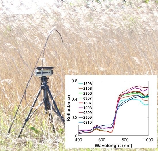
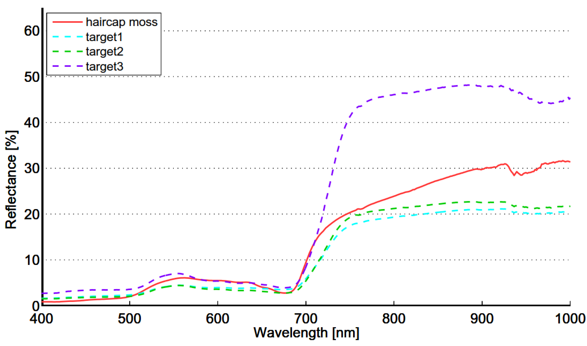
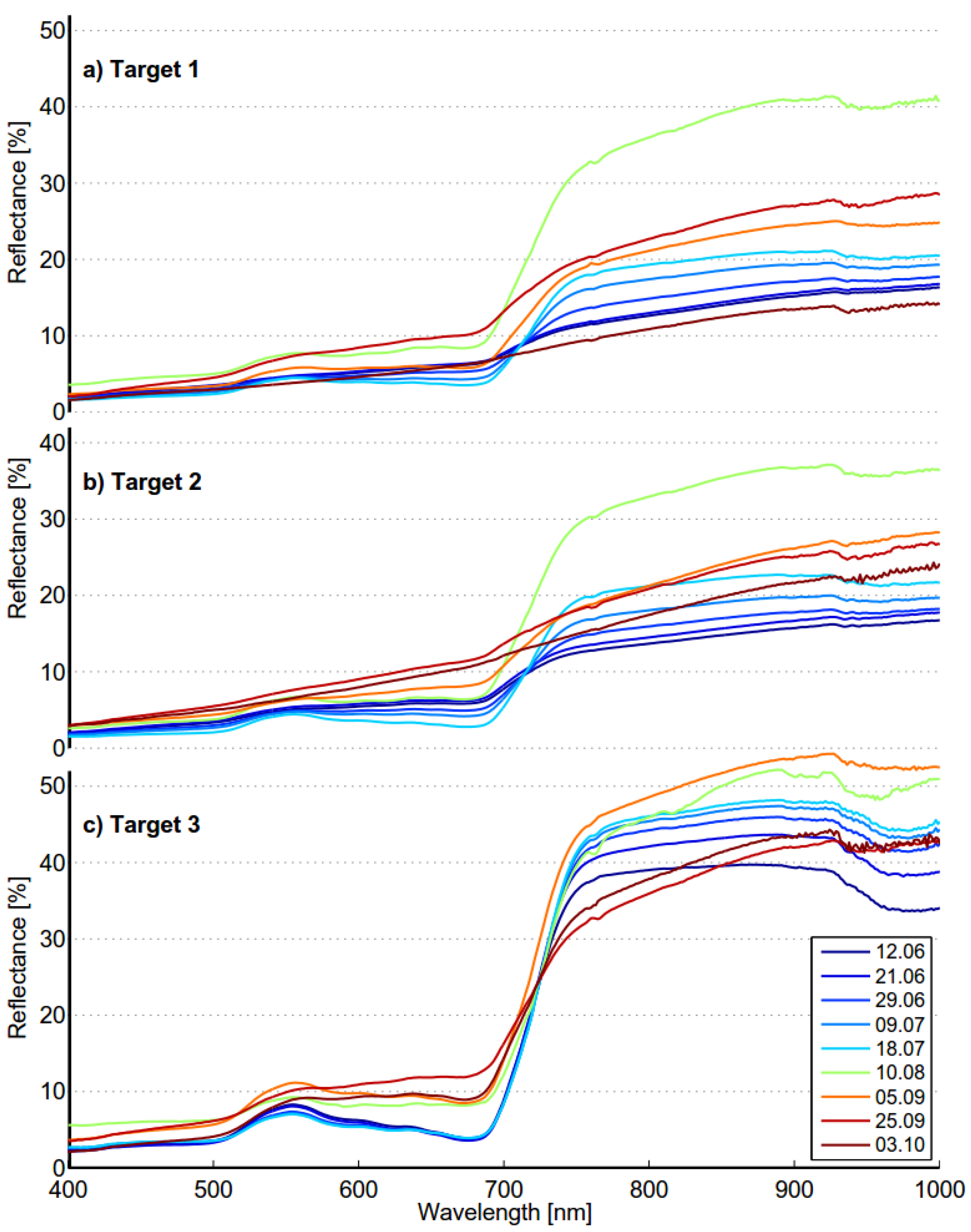
Several seasonal time-series spectra of Phragmites have been published in the literature. Seasonal spectra are dependent on local conditions, but spectral features reflecting phenological stages should be found in time-series spectra anywhere. The seasonal spectra of targets 1 and 2 are quite consistent with those published by Ouyang et al. [19]. The shape of the spectra is quite similar at the beginning and the end of the season as well as in the “full vigor” state. The growth period is naturally somewhat shorter in Finland than in Dongtan, China. The seasonal spectra of target 3 differ from those in [19] at the beginning and end of the season. The seasonal spectra of targets 1 and 2 show similar trends as those found in time-series spectra of Phragmites measured in New Jersey Meadowlands [20]. When seasonal spectra were compared to those published by Gilmore et al. [26], the situation was quite the opposite: the published spectra were very similar to those of target 3 in our study. The results show that the optimal time for data acquisition is dependent on classification method to be used. For distance based classifier optimal time for old reed bed is in the middle of June when it is the beginning of September for new reed bed. Optimal times are different when shape based classifier is used; beginning of October for old reed bed and the middle of June for new reed bed. The separability of old reed bed is almost as high in the middle of June as in October. Acquisition in the middle of June could give good results for both reed bed types.

The seasonal spectral changes of targets 1, 2 and 3 are largely determined by two variables: density of the reed bed and the ratio of dead and live biomass. Density defines if the soil or water is visible. Dark soil and water have low reflectance, which lowers the mixed spectra. Dead biomass has low and flat spectrum, whereas live biomass has distinct features of green vegetation. In the beginning of season old reed beds have only a small fraction on live biomass and the soil is partly visible because of low density. The spectrum is low and flat and therefore separable from moss. In the beginning of October old reed beds are full of dead biomass, resulting similar flat spectrum and high separability from green vegetation. The spectra of moss show signs of moderate chlorophyll content, modest local maximum near 560 nm and gentle red-edge. Target 3 is in “full vigor” state on 5 September 2012, the reflectance in green and NIR region is at the season’s highest level and therefore the separability from moss is optimal.

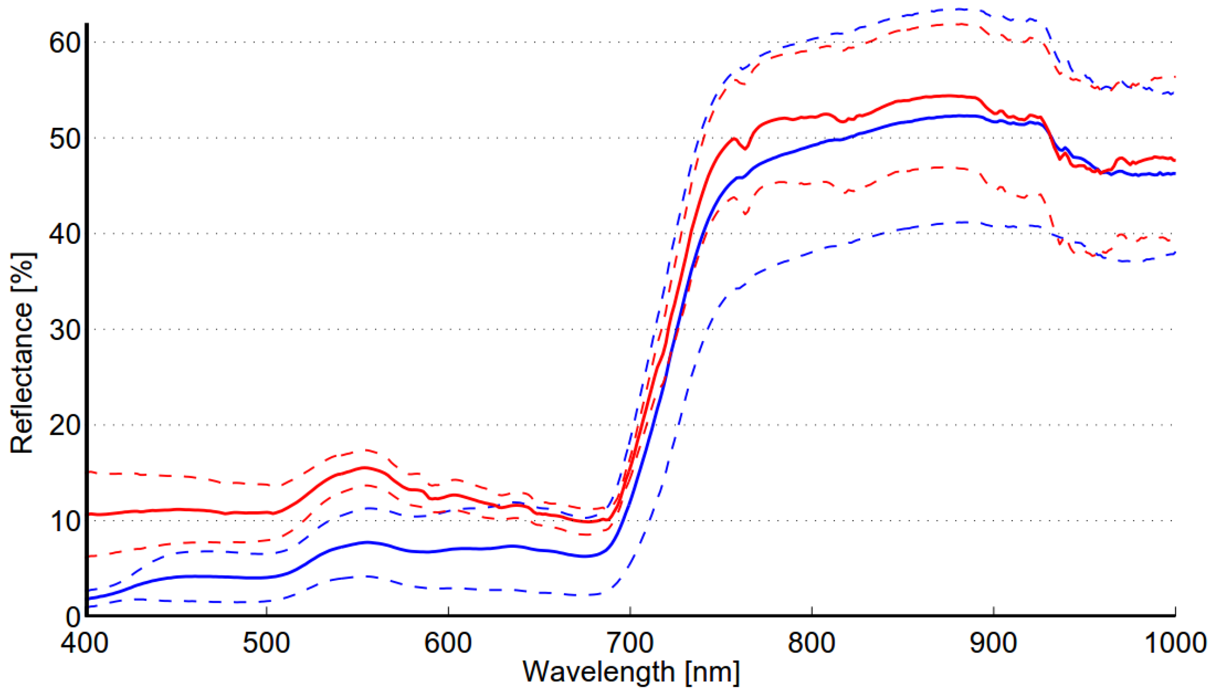
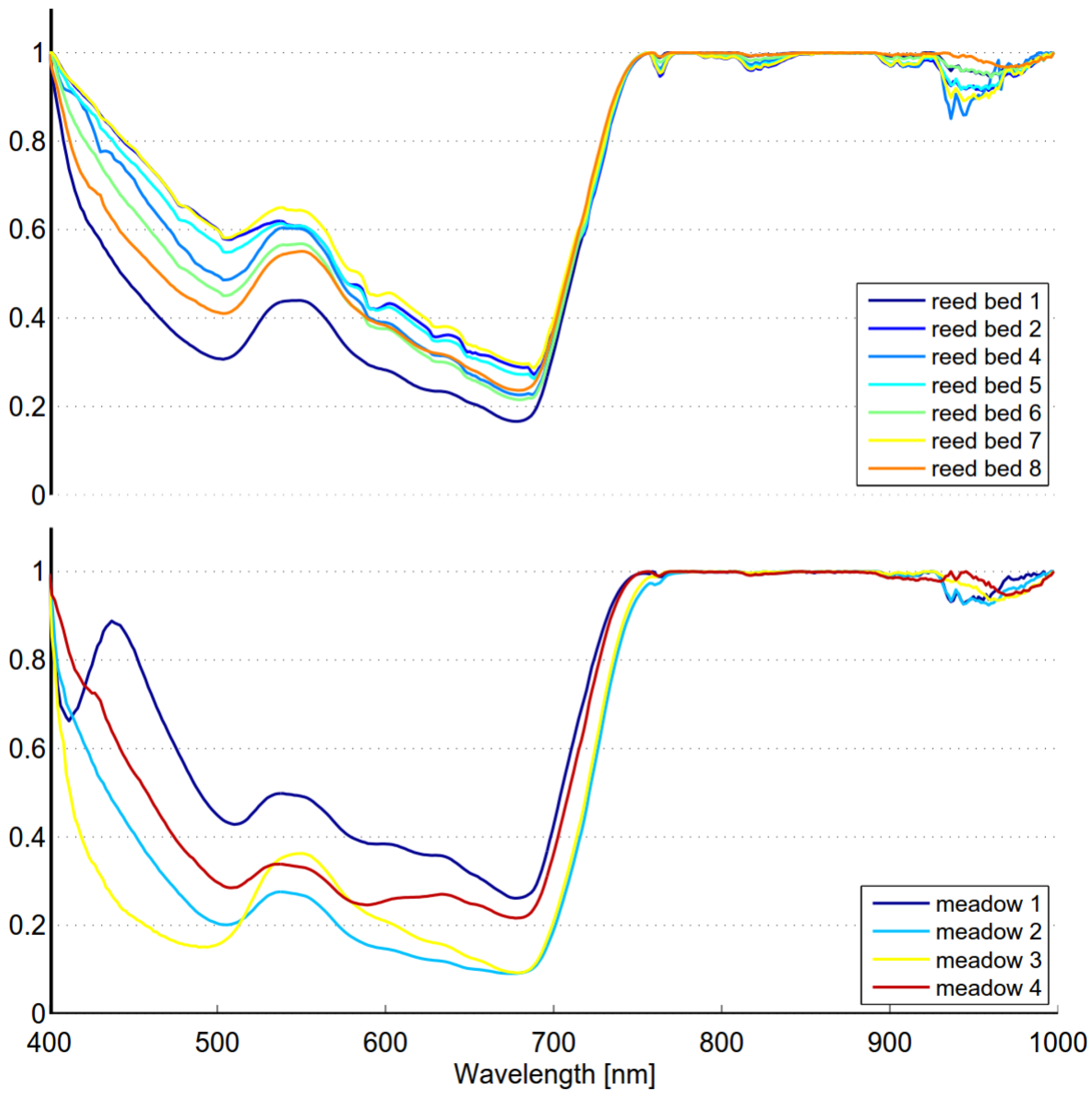
The within-class variability of reed is somewhat lower than that of the meadow class (see Table 8). This can be expected as the meadow class contains several species, i.e., grasses, weeds and flowers. The well-kept grass field was visually very homogenous; however, the spectral variability obtained for this class is higher than could be expected. This is most likely due the structural changes in grass. Results indicate that a single target (R1) significantly contributes to the within-class variability of the reed class. Debba et al. [31] studied the spectral within-class variability of different savannah trees. The average variability of seven tree species was lower than that of reed in this study. The published reflectance spectra of tree species showed that the within-class variability of some species (Combretum apiculatum, Terminalia sericia) was at the same level as obtained here for reed, although the average variability over all species was lower. Based on the analysis of the mean and standard deviation of the spectra obtained for the reed and meadow classes (see Figure 5) it is fair to argue that the two classes are extremely difficult to discriminate due to high within-class variability of both classes as well as spectral similarity of the classes. Several published studies have proposed fusion of hyperspectral and LiDAR data in wetlands mapping applications [16]. LiDAR can complement the spectral information of optical imagery and thus improve classification results. As the height of reed beds clearly differs from that of meadows, such approach could be highly beneficial. In addition, using textural features together with spectral information has been shown to enhance the classification accuracy of remotely sensed data [32].

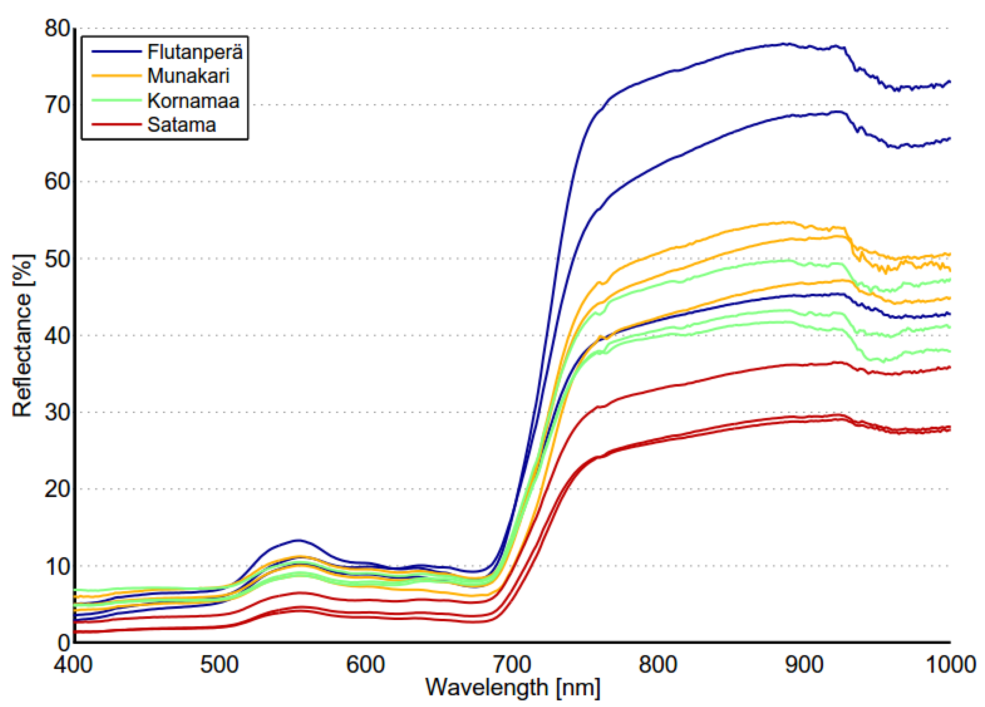
Spectral variability of reed beds within the Olkiluoto Island is significant (see Figure 7). Zomer et al. [33] studied the reflectance spectra of dominant wetland species. The measured results of common reed (Phragmites Australis) showed similar shape and high variability as in Figure 7. This suggests that high spectral variability could be common characteristics for reed beds. In order to study spectral variability between reed sites, each site was assigned to a separate class and between-class variability was calculated for each pair of sites. Surprisingly the between-class variability of sites Munakari and Kornamaa (3.85) was lower than local spatial inter-class variability of reed bed at site Pier (15.95). The between-class variability of these two sites was also lower than the variability between spectrally similar Savannah trees [31]. The highest variability was measured between sites Flutanperä and Satama. This is likely due to remarkable reflectance differences in the NIR region shown in Figure 7. 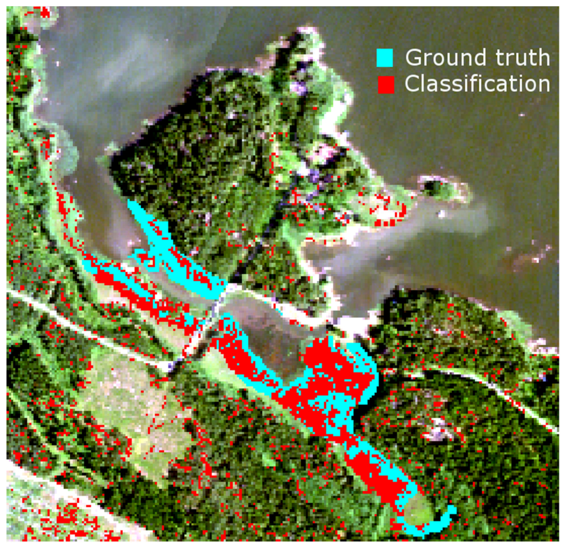This can be explained by the characteristics of reed beds presented in Table 2. The density and height of dead reed stems is clearly higher at Satama than at Flutanperä. The effects of spectral variability to reed bed discrimination within Olkiluoto Island were studied using airborne hyperspectral data. The accuracy of classification was measured using mean spectra of reed bed sites as a target spectra. Overall accuracy was good, mainly because the other class was much larger than reed bed class, i.e., the relative amount of commission errors stays low. The results of agreement accuracy were modest. This is most likely due to two factors: unfavorable time to separate reed beds from other vegetation and variety of reed bed types present, i.e., old, new and dry reed beds. Conventional remote sensing schemes use one reference spectrum for each species. The results suggest that the use of multiple-endmember approach might be beneficial, agreement accuracy increases when dedicated spectrum is used for reed bed site instead of using one spectrum for the whole island.

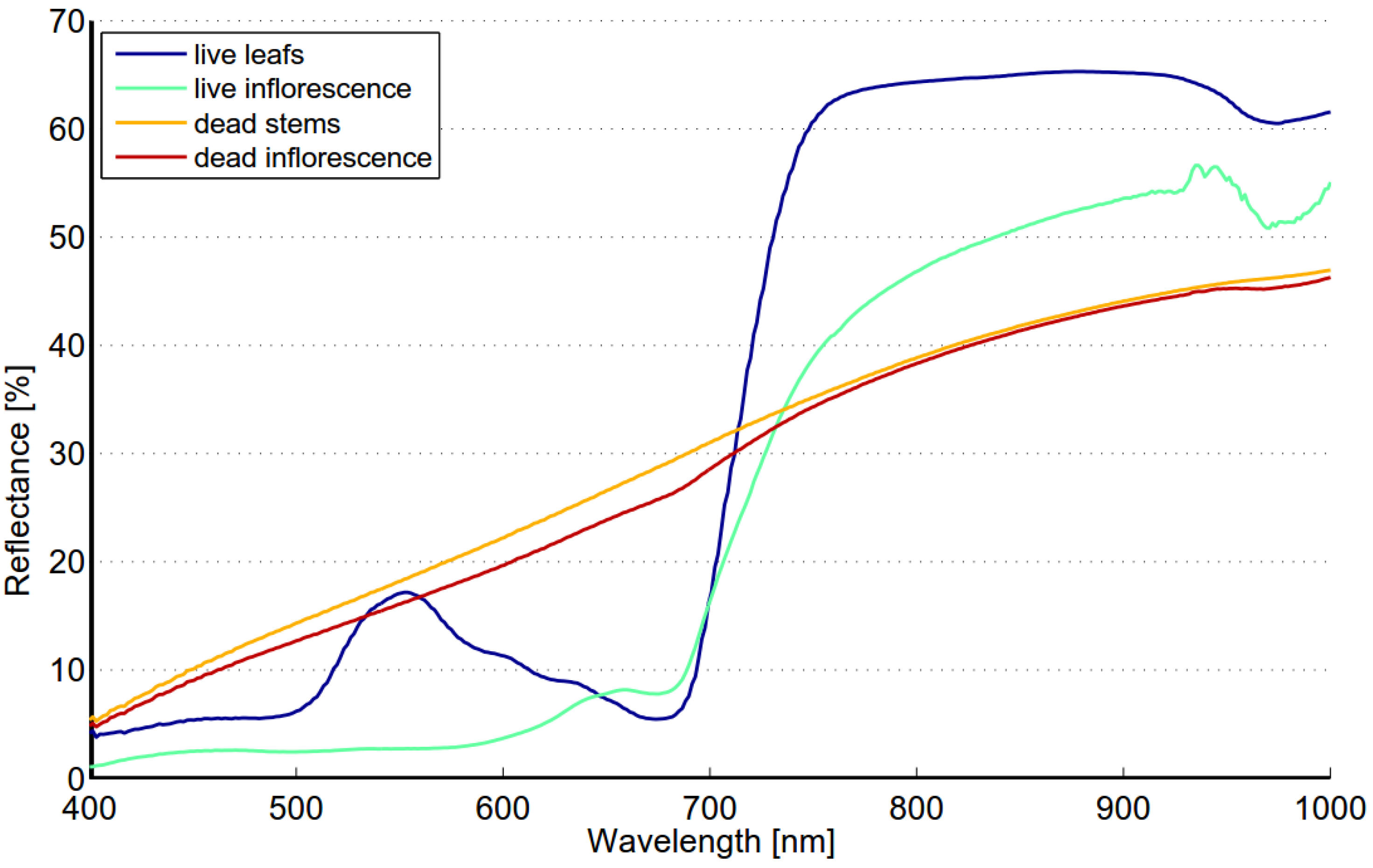
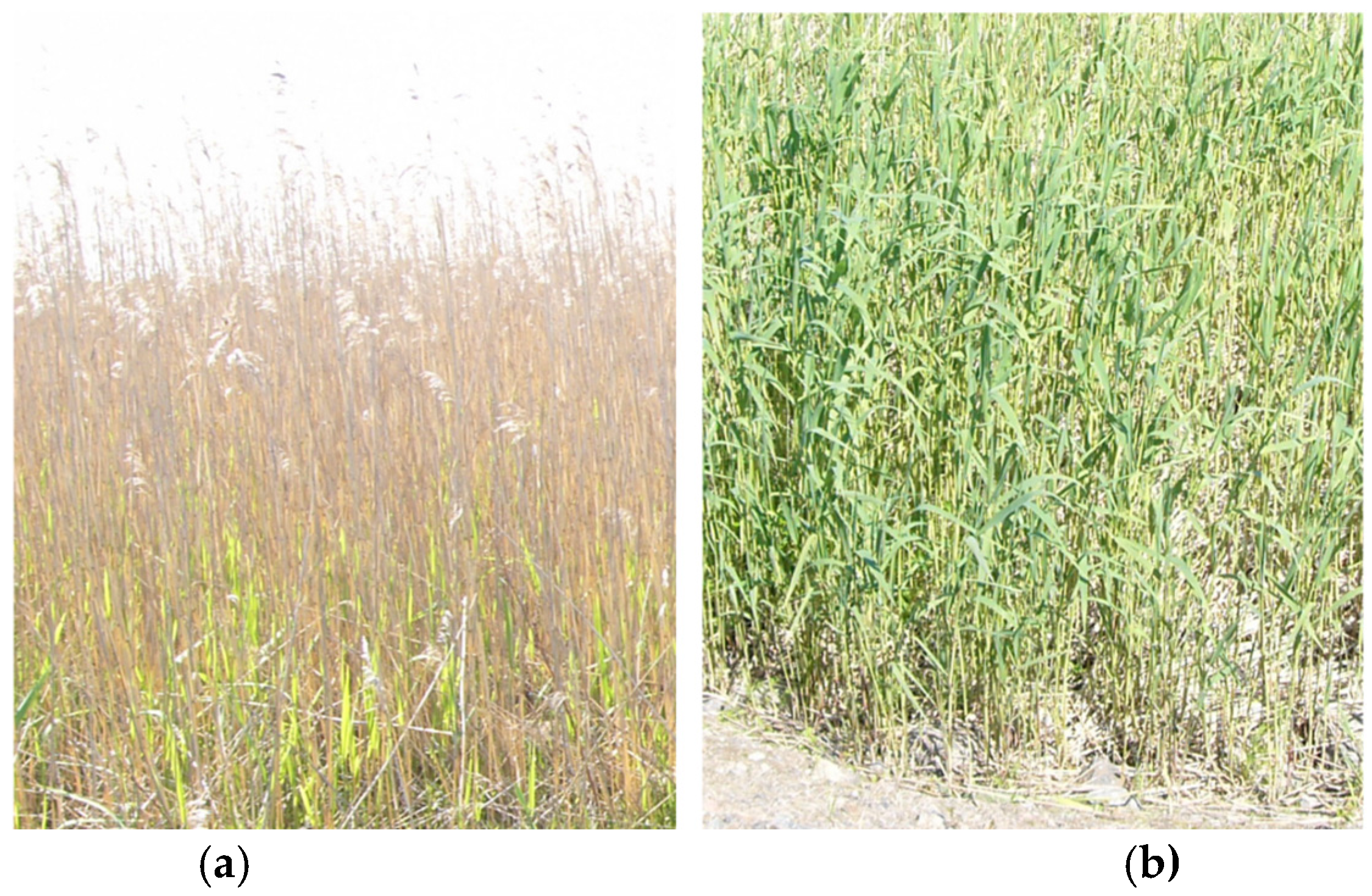
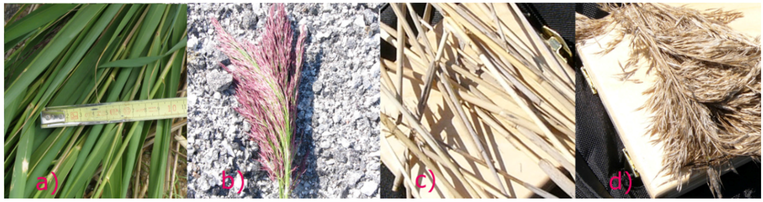
The spectrum of reed bed is largely determined by the density of reed stems and the ratio of live and dead biomass. The reed bed spectra may also include background contributions from water, soil, understory vegetation and shade depending on the density and structure of reed stems. Live leafs have typical spectrum of healthy green vegetation, i.e., steep red edge and reflectance peak near 560 nm while the spectrum of dead stems is flat and the reflectance level is low (Figure 9). The reflectance of a dead stem is higher in the NIR region when compared to autumn spectra of targets 1 and 2. This is most likely due to shadows between stems or visible soil/water or both. The spectrum of type “old reed bed” varies depending on the ratio of live and dead stems. Field studies made in August 2012 showed that there is considerable variability in the ratio of live and dead stems. The fraction of dead stems varied from 0 to 83%. The most obvious reason for high spectral variability within Olkiluoto Island is the changes in the ratio of live and dead stems.

5. Conclusions

The temporal and spatial variability of reed bed spectra was evaluated in this study. The temporal variability of reed bed spectra was found to be significant. The main challenge related to temporal variability is that there are two different types of reed beds having different seasonal spectra. The optimal time of data acquisition depends on the reed bed type. When this is combined with the fact that usually the phenological state of the other vegetation has to be considered as well, careful timing of the data acquisition is needed. The spectral within-class variability of both reed bed and meadow in local neighborhood was found to be large when compared to references. Both classes have similar mean spectra, however, all the targets except R1 had lower spectral angle to the mean spectrum of the corresponding class than that of the other class. This gives a positive indication for successful reed bed mapping. The results on within-class spectral variability of reed bed at four test sites within the Olkiluoto Island showed that while the reed spectra from the sites of Kornamaa and Munakari were close to each other, the spectra measured at Satama and Flutanperä differed significantly. This is at least partly due to the variation in the density and height of live and dead reed stems among the four sites. It can be concluded that if features such as reed characteristics, temporal variation and surrounding habitats are known and can be controlled, mapping of reed beds is feasible based on their spectral properties; otherwise LiDAR data or textural features would be needed.

In this study, the optimal times to separate reed beds from other vegetation was determined. Depending on the reed bed types present and classification method to be used, it might be beneficial to use multi-temporal classification, i.e., use several dataset collected at different times. High spectral within-species variability measured advocates the use of multiple-endmember methods. The test using airborne hyperspectral data further supports this conclusion. Scaling from spectral field measurements to airborne/satellite data brings with it new challenges. Poor spatial resolution can lead to significant amount of mixed pixels confusing the classification process. Modest signal-to-noise ratio of satellite sensors can further increase this confusion. The spectral resolution of spaceborne multispectral sensors might be too low to differentiate to subtle differences between reed beds and other wetland vegetation. The study using spectral field measurements showed poor separability between reed beds and meadows when distance and statistical measures where used although better results were obtained using a SAM-measure. The errors in geometric, radiometric and atmospheric correction related to air- and spaceborne sensors can deteriorate this subtle separability. This study provides a sound basis for future research of reed bed discrimination using air- and spaceborne data.

References

1. Altartouri, A.; Nurminen, L.; Jolma, A. Modeling the role of the close-range effect and environmental variables in the occurrence and spread of Phragmites australis in four sites on the Finnish coast of the Gulf of Finland and the Archipelago Sea. Ecol. Evol. 2014, 4, 987–1005. [Google Scholar] [CrossRef] [PubMed]
2. Kern, J.; Idler, C. Treatment of domestic and agricultural wastewater by reed bed systems. Ecol. Eng. 1999, 12, 13–25. [Google Scholar] [CrossRef]
3. Köbbing, J.F.; Thevs, N.; Zerbe, S. The utilisation of reed (Phragmites australis): A review. Mires Peat 2013, 13, 1–14. [Google Scholar]
4. Hansson, P.A.; Fredriksson, H. Use of summer harvested common reed (Phragmites australis) as nutrient source for organic crop production in Sweden. Agric. Ecosyst. Environ. 2004, 102, 365–375. [Google Scholar] [CrossRef]
5. Fyfe, S.K. Spatial and temporal variation in spectral reflectance: Are seagrass species spectrally distinct? Limnol. Oceanogr. 2003, 48, 464–479. [Google Scholar] [CrossRef]
6. Cho, M.A.; Debba, P.; Mathieu, R.; Naidoo, L.; Van Aardt, J.; Asner, G.P. Improving discrimination of savanna tree species through a multiple-endmember spectral angle mapper approach: Canopy-level analysis. IEEE Trans. Geosci. Remote Sens. 2010, 48, 4133–4142. [Google Scholar] [CrossRef]
7. Price, J.C. How unique are spectral signatures? Remote Sens. Environ. 1994, 49, 181–186. [Google Scholar] [CrossRef]
8. Clark, M.; Roberts, D.; Clark, D. Hyperspectral discrimination of tropical rain forest tree species at leaf to crown scales. Remote Sens. Environ. 2005, 96, 375–398. [Google Scholar] [CrossRef]
9. Schmidt, K.S.; Skidmore, A.K. Spectral discrimination of vegetation types in a coastal wetland. Remote Sens. Environ. 2003, 85, 92–108. [Google Scholar] [CrossRef]
10. Thenkabail, P.S. Optimal hyperspectral narrowbands for discriminating agricultural crops. Int. J. Remote Sens. 2001, 20, 257–291. [Google Scholar] [CrossRef]
11. Vahtmäe, E.; Kutser, T.; Martin, G.; Kotta, J. Feasibility of hyperspectral remote sensing for mapping benthic macroalgal cover in turbid coastal waters—A Baltic Sea case study. Remote Sens. Environ. 2006, 101, 342–351. [Google Scholar] [CrossRef]
12. Ramsey, E.; Rangoonwala, A. Hyperspectral remote sensing of wetland vegetation. In Hyperspectral Remote Sensing of Vegetation; Taylor & Francis: Abingdon, UK, 2011; pp. 487–511. [Google Scholar]
13. Adam, E.; Mutanga, O.; Rugege, D. Multispectral and hyperspectral remote sensing for identification and mapping of wetland vegetation: A review. Wetl. Ecol. Manag. 2010, 18, 281–296. [Google Scholar] [CrossRef]
14. Pengra, B.W.; Johnston, C.A.; Loveland, T.R. Mapping an invasive plant, Phragmites australis, in coastal wetlands using the EO-1 Hyperion hyperspectral sensor. Remote Sens. Environ. 2007, 108, 74–81. [Google Scholar] [CrossRef]
15. Lopez, R.; Edmonds, C.; Neale, A.; Slonecker, T.; Jones, B.; Heggem, T.; Lyon, J.; Jaworski, E.; Garofalo, D.; Williams, D. Accuracy assesments of airborne hyperspectral data for mapping opportunistic plant species in freshwater coastal wetlands. In Remote Sensing and GIS Accuracy Assessment; Taylor & Francis: Abingdon, UK, 2007; pp. 318–339. [Google Scholar]
16. Onojeghuo, A.O.; Blackburn, G.A. Optimising the use of hyperspectral and LiDAR data for mapping reedbed habitats. Remote Sens. Environ. 2011, 115, 2025–2034. [Google Scholar] [CrossRef]
17. Stratoulias, D.; Balzter, H.; Zlinszky, A.; Tóth, V.R. Assessment of ecophysiology of lake shore reed vegetation based on chlorophyll fluorescence, field spectroscopy and hyperspectral airborne imagery. Remote Sens. Environ. 2015, 157, 72–84. [Google Scholar] [CrossRef] [Green Version]
18. Goetz, A.F.H. Three decades of hyperspectral remote sensing of the Earth: A personal view. Remote Sens. Environ. 2009, 113, S5–S16. [Google Scholar] [CrossRef]
19. Ouyang, Z.T.; Gao, Y.; Xie, X.; Guo, H.Q.; Zhang, T.T.; Zhao, B. Spectral discrimination of the invasive plant spartina alterniflora at multiple phenological stages in a Saltmarsh Wetland. PLoS ONE 2013, 8, 1–12. [Google Scholar] [CrossRef] [PubMed]
20. Artigas, F.J.; Yang, J.S. Hyperspectral remote sensing of marsh species and plant vigour gradient in the New Jersey Meadowlands. Int. J. Remote Sens. 2005, 26, 5209–5220. [Google Scholar] [CrossRef]
21. Van der Meer, F. The effectiveness of spectral similarity measures for the analysis of hyperspectral imagery. Int. J. Appl. Earth Obs. Geoinformation 2006, 8, 3–17. [Google Scholar] [CrossRef]
22. Haapanen, R.; Lahdenperä, A.M. The Inventory of the Terrestrial Part of Land-To-Sea Transects on Olkiluoto Island in 2008 and the Investigations of Reedbeds Surrounding Olkiluoto Island Carried out in 2007–2008; Posiva Ltd.: Eurajoki, Finland, 2011. [Google Scholar]
23. Kangasniemi, V.; Helin, J. Studies on the Aquatic Environment at Olkiluoto and Reference Area: 1. Olkiluoto, Reference Lakes and Eurajoki and Lapijoki Rivers in 2009–2010; Posiva Ltd.: Eurajoki, Finland, 2014. [Google Scholar]
24. Pohjola, J.; Turunen, J.; Lipping, T.; Ikonen, A.T.K. Computers and geosciences landscape development modeling based on statistical framework. Comput. Geosci. 2014, 62, 43–52. [Google Scholar] [CrossRef]
25. Lambertini, C.; Gustafsson, M.H.G.; Frydenberg, J.; Speranza, M.; Brix, H. Genetic diversity patterns in Phragmites australis at the population, regional and continental scales. Aquat. Bot. 2008, 88, 160–170. [Google Scholar] [CrossRef]
26. Gilmore, M.S.; Wilson, E.H.; Barrett, N.; Civco, D.L.; Prisloe, S.; Hurd, J.D.; Chadwick, C. Integrating multi-temporal spectral and structural information to map wetland vegetation in a lower Connecticut River tidal marsh. Remote Sens. Environ. 2008, 112, 4048–4060. [Google Scholar] [CrossRef]
27. Kruse, F.A.; Lefkoff, A.B.; Boardman, J.W.; Heidebrecht, K.B.; Shapiro, A.T.; Barloon, P.J.; Goetz, A.F.H. The spectral image proccessing system (SIPS)—Interactive visualization and analysis of imaging spectrometer data. Remote Sens. Environ. 1993, 44, 145–163. [Google Scholar] [CrossRef]
28. Swain, P.H.; Davis, S. Remote Sensing: The Quantatitative Approach; McGraw Hill Book Company: New York, NY, USA, 1978. [Google Scholar]
29. Kokaly, R.F. Investigating a physical basis for spectroscopic estimates of leaf nitrogen concentration. Remote Sens. Environ. 2001, 75, 153–161. [Google Scholar] [CrossRef]
30. Canty, M.J. Image Analysis, Classification, and Change Detection in Remote Sensing: With Algorithms for ENVI/IDL; CRC Press: Boca Raton, FL, USA, 2010. [Google Scholar]
31. Debba, P.; Cho, M.A.; Mathieu, R. Within- and between-class variability of spectrally similar tree species. In Proceedings of the 2009 IEEE International Geoscience and Remote Sensing Symposium, Cape Town, South Africa, 12–17 July 2009; Volume 4, pp. 272–275.
32. Onojeghuo, A.O.; Blackburn, G.A. Mapping reedbed habitats using texture-based classification of QuickBird imagery. Int. J. Remote Sens. 2011, 32, 8123–8138. [Google Scholar] [CrossRef]
33. Zomer, R.J.; Trabucco, A.; Ustin, S.L. Building spectral libraries for wetlands land cover classification and hyperspectral remote sensing. J. Environ. Manag. 2009, 90, 2170–2177. [Google Scholar] [CrossRef] [PubMed]
Figure 1. Overview of the study sites Olkiluoto (left) and Hilskansaari (right).
Remotesensing 08 00181 g001
Figure 2. Old reed bed of target 2 (a) and new reed bed of target 3 (b). The photographs are taken on 12 June 2012.
Remotesensing 08 00181 g002
Figure 3. The measured spectra of targets 1, 2 and 3 during the growth period. The measurement dates are shown in the legend. (a) Target 1; (b) Target 2; (c) Target 3.
Remotesensing 08 00181 g003
Figure 4. The reference spectrum of haircap moss and the spectra of targets 1–3 measured on 18 July 2012.
Remotesensing 08 00181 g004
Figure 5. Mean and standard deviation of the reflectance spectra of meadow (blue) and reed bed (red) classes. The standard deviation is presented using dashed lines.
Remotesensing 08 00181 g005
Figure 6. Continuum removed spectra of reed bed and meadow classes.
Remotesensing 08 00181 g006
Figure 7. The reed bed reflectance spectra at the four test sites in Olkiluoto Island.
Remotesensing 08 00181 g007
Figure 8. Samples of measured reed components: (a) live leafs; (b) live inflorescence; (c) dead stems; and (d) dead inflorescence.
Remotesensing 08 00181 g008
Figure 9. The partial spectra of reed bed.
Remotesensing 08 00181 g009
Figure 10. The classification results using the mean spectrum of Kornamaa.
Remotesensing 08 00181 g010