Computationally Inexpensive Landsat 8 Operational Land Imager (OLI) Pansharpening

Abstract

Pansharpening algorithms fuse higher spatial resolution panchromatic with lower spatial resolution multispectral imagery to create higher spatial resolution multispectral images. The free-availability and systematic global acquisition of Landsat 8 data indicate an expected need for global coverage and so computationally efficient Landsat 8 pansharpening. This study adapts and evaluates the established, and relatively computationally inexpensive, Brovey and context adaptive Gram Schmidt component substitution (CS) pansharpening methods for application to the Landsat 8 15 m panchromatic and 30 m red, green, blue, and near-infrared bands. The intensity images used by these CS pansharpening methods are derived as a weighted linear combination of the multispectral bands in three different ways using band spectral weights set (i) equally as the reciprocal of the number of bands; (ii) using fixed Landsat 8 spectral response function based (SRFB) weights derived considering laboratory spectra; and (iii) using image specific spectral weights derived by regression between the multispectral and the degraded panchromatic bands. The spatial and spectral distortion and computational cost of the different methods are assessed using Landsat 8 test images acquired over agricultural scenes in South Dakota, China, and India. The results of this study indicate that, for global Landsat 8 application, the context adaptive Gram Schmidt pansharpening with an intensity image defined using the SRFB spectral weights is appropriate. The context adaptive Gram Schmidt pansharpened results had lower distortion than the Brovey results and the least distortion was found using intensity images derived using the SRFB and image specific spectral weights but the computational cost using the image specific weights was greater than the using the SRFB weights. Recommendations for large area Landsat 8 pansharpening application are described briefly and the SRFB spectral weights are provided so users may implement computationally inexpensive Landsat 8 pansharpening themselves.

1. Introduction

Moderate to very high spatial resolution satellite remote sensing systems typically include multi-spectral bands, designed primarily for surface classification applications, and a higher spatial but lower spectral resolution panchromatic band designed for positioning and mensuration applications. If the panchromatic band is spectrally overlapping with several of the multi-spectral bands then the multi-spectral bands may be pansharpened to provide a panchromatic spatial resolution equivalent [1,2,3,4]. Some studies have also considered pansharpening multi-spectral bands that do not overlap spectrally with the panchromatic band [5,6]. Ideally, pansharpening is undertaken in a way that introduces minimal spatial and spectral distortion into the pansharpened data. There is no consensus pansharpening technique, primarily because spectral and spatial distortions are dependent on the heterogeneity of the sensed surface features and on the sensor characteristics and because of among sensor differences.

The free-availability and systematic global acquisition of Landsat data [7,8] combined with increases in computational and data storage capabilities mean that it is now feasible to process large-area, long-term, large volume Landsat data sets [9,10,11]. For example, global coverage, monthly and annual Web Enabled Landsat data (WELD) 30 m monthly and annual composited mosaics have been processed and are now freely available (http://globalweld.cr.usgs.gov/collections/). Pansharpened data are frequently used for internet based visualization and mapping [12] and recently pansharpened Landsat 7 Enhanced Thematic Mapper Plus (ETM+) were used to produce a global coverage 14.25 m water body database [13]. Global coverage pansharpened Landsat data should be derived using computationally efficient pansharpening algorithms given the considerable Landsat data volume. As of January 2015, there were more than 5.5 million Landsat images stored in the U.S. archive with an additional 2.3 million historical images held by other agencies that will be added [8]. The Landsat 8 satellite continues the 40+ year Landsat data record [14]. The Landsat 8 Operational Land Imager (OLI) has improved calibration, signal to noise characteristics, higher 12-bit radiometric resolution and more precise geometry compared to previous Landsat reflective wavelength sensors, and the 15 m panchromatic band covers only the visible wavelengths to provide improved contrast between vegetated and bare surfaces [15]. In this study, we seek to develop a computationally efficient Landsat 8 OLI pansharpening algorithm suitable for very large OLI data application that can be used to pansharpen the 30 m red, green, blue, and near-infrared OLI bands.

Pansharpening methods may be classified into component substitution, multi-resolution analysis, and model-based methods [16,17,18,19]. Component substitution (CS) methods are considered in this paper as they are computationally efficient and perform similarly to other methods [6,20,21,22]. CS pansharpening methods are implemented in several steps to derive:

(i)

a band intensity image at the multispectral band resolution, typically as a weighted linear combination of the multispectral band values;

(ii)

a pan spatial resolution spatial detail image by subtracting the intensity image from the panchromatic band;

(iii)

a pan spatial resolution modulated spatial detail image for each multispectral band as the product of the pan spatial detail image and a locally adaptive, or fixed, scalar modulation coefficient;

(iv)

for each multispectral band a pansharpened equivalent by adding the multispectral band to the band’s modulated spatial detail image.

In this study the well established Brovey [23] and context adaptive Gram Schmidt [18] pansharpening methods, that have been shown to introduce less spatial and spectral distortion than other CS methods, and that are computationally relatively inexpensive, are considered. A novel OLI intensity image derivation method (step (i) above) based on the OLI band spectral response functions and laboratory spectra is examined along with more conventional intensity derivation approaches.

The Landsat 8 satellite OLI sensor data and the spectral measurements used to test and develop the pansharpening methods are first described. Then the process to derive a single band intensity image as a linear function of the Landsat red, green and blue band spectral weights, and also as a function of only the red and green Landsat band spectral weights, is described. The spectral weights used to derive the intensity images are defined in three different ways (i) fixed equal spectral weights; (ii) fixed spectral weights derived considering laboratory spectra and the Landsat 8 OLI spectral response functions; and (iii) image specific spectral weights derived using a regression between the multispectral and the degraded panchromatic band [24]. Resampling of the Landsat 8 OLI data from 30 m to 15 m is then described followed by description of the Brovey and context adaptive Gram Schmidt pansharpening methods and the pansharpening evaluation methodology. Quantitative and qualitative evaluation results for the visible and NIR bands of three test Landsat 8 OLI images are reported, with consideration of the computational efficiency of the different pansharpening methods, prior to concluding remarks.

2. Data

2.1. Landsat 8 Data

The spectral response functions for the Landsat 8 OLI bands used in this study (Figure 1) are described in [25] and were obtained from [26]. The visible wavelength OLI 30 m red (0.636–0.673 µm), green (0.533–0.590 µm), blue (0.452–0.512 µm), and near-infrared (NIR, 0.851–0.879 µm) bands and the 15 m panchromatic band (0.503–0.676 µm) were used. The panchromatic band covers only visible wavelengths to provide greater contrast between vegetated and bare surfaces [15] and overlaps spectrally with the green and red bands but only marginally with the blue band, and not at all with the NIR band. The blue, green and red band spectral response functions intersect with 5.2%, 32.8% and 22.8% of the panchromatic band spectral response function respectively. Conversely, the panchromatic band spectral response function intersects with 14.9%, 94.1% and 99.6% of the blue, green and red band functions respectively.

Landsat 8 data are available in approximately 190 km × 180 km scenes defined in the second World-wide Reference System (WRS-2) of scene path (ground track parallel) and row (latitude parallel) coordinates [27]. Standard Level 1T processing includes radiometric correction, systematic geometric correction, precision correction using ground control chips, and the use of a digital elevation model to correct parallax error due to local topographic relief. The Landsat 8 L1T product has a band-to-band registration accuracy of less than 4.5 m for the OLI bands, i.e., better than the panchromatic band pixel dimensions, and a circular geolocation error uncertainty requirement of <12 m [15].

Three largely cloud-free Landsat 8 L1T images acquired over South Dakota, China, and India that provide a range of radiometric and geometric features for testing the pansharpening algorithms were selected. The images were acquired over predominantly agricultural regions, with variable field sizes and patterns, and include settlements and distinct road networks. A single rectangular spatial subset was extracted from each L1T image, ensuring that each subset contained no cloudy pixels and no scene edges. Specifically, spatial subsets with 30 m pixel dimensions of 2734 × 2532 (South Dakota), 2976 × 2520 (China), and 2970 × 2470 (India) were extracted. These data were converted into top of atmosphere reflectance (unitless, range 0–1) using the L1T image metadata.

The South Dakota image was located over the authors’ university town, Brookings, central eastern South Dakota, WRS-2 path 29/row 29, and was sensed 29 June 2014. The main crops are corn and soybean grown in large fields with side dimensions of the order of tens to hundreds of 30 m pixels [28]. The China image was WRS-2 path 123/row 36 located in Henan province, in the North China Plain, sensed 1 September 2013. Like much of rural China, the image is dominated by small scale intensive farming with predominantly winter wheat and rice crops [29,30] and contains many long rectangular fields including rice fields with small axes dimensions that can be smaller than the Landsat 30 m pixel dimension [31]. The India image was acquired over WRS-2 path 148/row 39 located over north west India in the state of Punjab, and was sensed 31 August 2103. In this region predominantly rice and cotton crops grow in the Summer followed by winter wheat planted later in Autumn and harvested in Spring [32,33,34]. The Indian image field sizes are comparable and slightly larger than those in the China image.

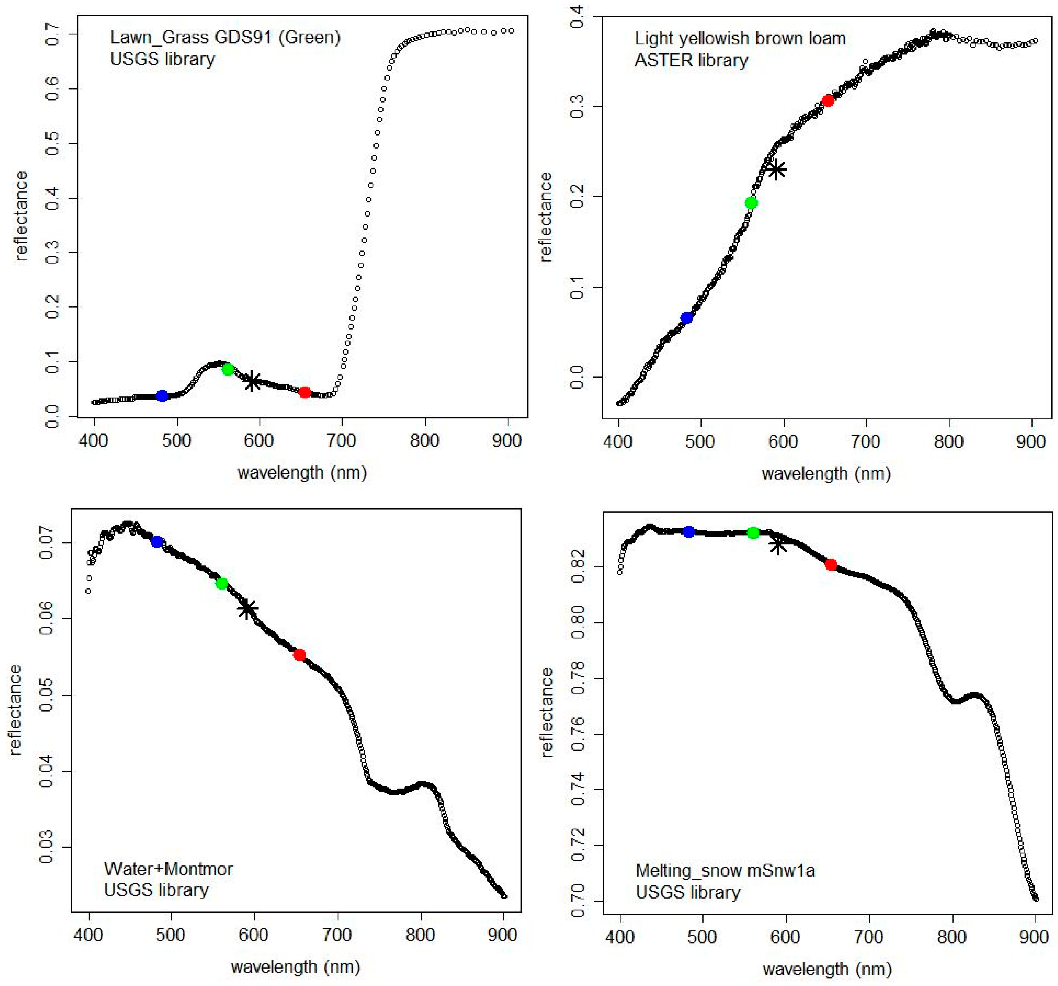
2.2. Spectral Library Data

Spectral measurements were used to simulate Landsat 8 reflectance values needed to develop spectral response function based (SRFB) spectral weights (Section 3.1.2). Vegetation, soil, water, ice and snow spectra from three spectral libraries were used, namely, the Version 6 USGS spectral library [35], the Version 2 ASTER spectral library [36], and the Jasper Ridge spectral library [37]. Only the visible and near-infrared (VNIR) data from 0.4 to 0.9 µm were used. The VNIR USGS spectral library data were measured with a Beckman 5270 spectrophotometer, an Analytical Spectral Devices (ASD) portable field spectrometer, and derived from atmospherically corrected NASA Airborne Visible/Infra-Red Imaging Spectrometer (AVIRIS) data. The VNIR ASTER spectral library data were measured with a Beckman UV5240 spectrophotometer and a Perkin-Elmer Lambda 900 UV/VIS/NIR spectrophotometer. The VNIR Jasper Ridge spectral library data were measured with a Beckman UV5240 spectrophotometer. The sample intervals of the Perkin-Elmer Lambda 900, ASD and AVIRIS measurements were 1 nm, 1 nm and 10 nm respectively. The sample interval of the two Beckman instruments was 1 nm in the visible and 4 nm in the NIR wavelength range [36].

The spectra are provided with cover type descriptions. However, for this study, to unambiguously differentiate between vegetation and soil spectra the normalized difference vegetation index (NDVI) was computed and only vegetation spectra with NDVI ≥0.2 were selected. Similarly, only soil spectra with NDVI <0.2 were selected. This provided a total of 335 spectra (270 vegetation, 34 soil, 10 water, and 21 snow and ice spectra). The NDVI was computed for each spectra as the simulated OLI NIR (0.845–0.885 µm) reflectance minus the simulated OLI red reflectance (0.640–0.670 µm) divided by their sum. The OLI band simulation is described in Section 3.1.

3. Methods

3.1. Single Band Intensity Image Derivation

The first step in pansharpening is the derivation of a single band intensity image that is similar to the panchromatic band but is defined at the multispectral band spatial resolution as a weighted linear combination of the multispectral band values. In this study, red, green and blue spectral weights Equation (1) were considered. The NIR band was not used to derive the intensity image as it does not overlap spectrally with the panchromatic band. In addition, just red and green spectral weights Equation (2) were considered as the panchromatic band overlaps only marginally with the blue band (Figure 1) and because the Landsat blue band is very sensitive to atmospheric effects and is not usually reliably atmospherically corrected [14,38,39].

$$\begin{array}{cc}I(\mathrm{i},\mathrm{j})=& w_{red}{\rho }_{red}(\mathrm{i},\mathrm{j})\end{array}+w_{green}{\rho }_{green}(\mathrm{i},\mathrm{j})+w_{blue}{\rho }_{blue}(\mathrm{i},\mathrm{j})$$

(1)

$$\begin{array}{cc}I(\mathrm{i},\mathrm{j})=& w_{red}{\rho }_{red}(\mathrm{i},\mathrm{j})\end{array}+w_{green}{\rho }_{green}(\mathrm{i},\mathrm{j})$$

(2)

where $I(\mathrm{i},\mathrm{j})$ is the single band intensity image reflectance value at 30 m pixel location (i,j); ${\rho }_{red}(\mathrm{i},\mathrm{j})$, ${\rho }_{green}(\mathrm{i},\mathrm{j})$, and ${\rho }_{blue}(\mathrm{i},\mathrm{j})$ are the Landsat 8 30 m red, green and blue reflectance values, and $w_{red}$, $w_{green}$, and $w_{blue}$ are the spectral weights for these bands.

The spectral weights used to derive the intensity images were defined in three different ways (i) fixed equal spectral weights; (ii) fixed spectral weights derived considering laboratory spectra and the Landsat 8 OLI spectral response functions; and (iii) image specific spectral weights derived using a regression between the multispectral and the degraded panchromatic band [24]. These are described below.

3.1.1. Equal Spectral Weights

The simplest approach is to assign fixed equal spectral weights set as the reciprocal of the number of multispectral bands. Accordingly, in this study, equal spectral weights ($w_{red}$ = $w_{green}$ = $w_{blue}$ = ⅓ for Equation (1) and $w_{red}$ = $w_{green}$ = ½ for Equation (2)) were used to derive the intensity image. This approach implicitly assumes to first order that the surface reflectance changes linearly over the panchromatic and multispectral band wavelengths. This is not usually true, for example, Figure 2 illustrates vegetation, soil, water and snow library spectra (lines) that exhibit typical highly variable reflectance with wavelength.

3.1.2. Spectral Response Function Based (SRFB) Spectral Weights

Fixed spectral weights were derived by regression analysis of the simulated Landsat 8 OLI reflectance using the OLI band spectral response functions and the library spectra. First, simulated Landsat 8 OLI band reflectance values were calculated for each library spectrum [40] as:

$${\overline{\rho }}_{band}=\frac{{\displaystyle {\int }_{band{}_{\lambda \min }}^{band{}_{\lambda \max }}{s}_{band}(\lambda )\rho (\lambda )\mathrm{d}\lambda }}{{\displaystyle {\int }_{band{}_{\lambda \min }}^{band{}_{\lambda \max }}{s}_{band}(\lambda )\mathrm{d}\lambda }}$$

(3)

where ${\overline{\rho }}_{band}$ is the simulated reflectance for a specific Landsat 8 band (i.e., panchromatic, blue, green, or red), $s_{band}(\lambda )$ is the Landsat 8 band spectral response function (Figure 1), $band{}_{\lambda \min }$ and $band{}_{\lambda \max }$ are the minimum and maximum wavelengths where $s_{band}(\lambda )$ is greater than zero, and $\rho (\lambda )$ is the spectral library data for a give spectrum. The integration in Equation (3) was undertaken at 1 nm intervals for each library spectrum, linearly interpolating the reflectance values that were measured less frequently than 1 nm. Figure 2 illustrates example vegetation, soil, water and snow library spectra (lines) and the corresponding simulated Landsat 8 OLI panchromatic, red, green and blue band reflectance values (dots) in Equation (3). The small differences between the library spectral values at the OLI band center wavelengths and the simulated reflectance values are due to the higher spectral resolution of the library spectra relative to the OLI band spectral response functions.

Linear regressions of simulated Landsat 8 panchromatic reflectance against simulated red, green and blue reflectance band combinations were derived by ordinary least squares regression considering many spectra. Regressions considering red, green and blue reflectance, and also considering only red and green reflectance, were derived to provide relationships of the form:

$$\begin{array}{cc}{\overline{\rho }}_{pan}=& w_{red}{\overline{\rho }}_{red}\end{array}+w_{green}{\overline{\rho }}_{green}+w_{blue}{\overline{\rho }}_{blue}+\epsilon$$

(4)

$$\begin{array}{cc}{\overline{\rho }}_{pan}=& w_{red}{\overline{\rho }}_{red}+\end{array}{w}_{green}{\overline{\rho }}_{green}+\epsilon$$

(5)

where ${\overline{\rho }}_{pan}$, ${\overline{\rho }}_{red}$, ${\overline{\rho }}_{green}$, ${\overline{\rho }}_{blue}$ are simulated reflectances defined as Equation (3), and $w_{red}$, $w_{green}$, $w_{blue}$ are the regression coefficients that provide the spectral weights, and $\epsilon$ is the conventional regression error term, i.e., the difference between the simulated panchromatic reflectance and the linear combination of simulated multispectral reflectances, and the regression was derived by minimizing the sum of ${\epsilon }^2$.

The spectral response function based (SRFB) spectral weights were derived using a bootstrap sampling approach considering all the spectra but ensuring that an approximately equal number of spectra from each cover type were considered for the final weight derivation. Specifically, the 34 soil, 21 snow and ice, and 10 water spectra were considered with 34 vegetation spectra selected at random from the 270 vegetation spectra (i.e., a total of 99 spectra). This was repeated 100 times to derive 100 weights and the set of weights that was closest to the Euclidian center of the 100 groups of weights was derived to provide a single set of red, green and blue band SRFB weights, and a single set of red and green SRFB weights. In addition, to examine the influence of spectra variations among the different cover types the 335 spectra were grouped into vegetation, soil, snow and ice, and water, cover types and the weights were derived independently for each cover type.

3.1.3. Image Specific Spectral Weights

Rather than use fixed spectral weights, as described above, researchers have suggested the use of image specific weights that consider spectral relationships between bands [18,24]. This approach uses a regression between the multispectral and the degraded panchromatic band to derive the spectral weights for each image. A regression considering the 30 m red, green and blue reflectances and the spatially corresponding panchromatic reflectance degraded to 30 m were derived to provide a relationship of the form:

$$\begin{array}{cc}{\rho }_{pan}^L(\mathrm{i},\mathrm{j})=& w_{red}{\rho }_{red}(\mathrm{i},\mathrm{j})\end{array}+w_{green}{\rho }_{green}(\mathrm{i},\mathrm{j})+w_{blue}{\rho }_{blue}(\mathrm{i},\mathrm{j})+\epsilon$$

(6)

where ${\rho }_{pan}^L(\mathrm{i},\mathrm{j})$ is the degraded panchromatic reflectance at a 30 m pixel location (i,j), and ${\rho }_{red}(\mathrm{i},\mathrm{j})$, ${\rho }_{green}(\mathrm{i},\mathrm{j})$, ${\rho }_{blue}(\mathrm{i},\mathrm{j})$ are the 30 m red, green and blue reflectance values, and $w_{red}$, $w_{green}$, and $w_{blue}$ are the regression coefficients that provide the image specific spectral weights, and $\epsilon$ is the conventional regression error term.

Ideally, the 30 m degraded panchromatic reflectance should be derived by modelling the multispectral band point spread function (PSF) that describes the combined smoothing effects of the sensor detector electronics, optics, scanning mechanism, and atmospheric adjacency effects [41,42,43,44]. In this study, as the Landsat 8 OLI PSF for each band is unknown, a cubic-spline wavelet filter with a Gaussian-like frequency response followed by decimation was used to provide a first-order PSF approximation [45]. Unlike the equal and the SRFB spectral weights, the image specific weights are not constant among images.

3.2. Resampling Landsat 8 30 m Multispectral Bands to 15 m Panchromatic Pixel Grid

In order for the 30 m Landsat 8 multi-spectral bands to be pansharpened they, and the single band intensity images, were resampled to 15 m to align precisely with the 15 m panchromatic band. This is complicated because with Landsat 8 L1T data four 15 m pixels do not correspond spatially aligned to a 30 m pixel, rather the panchromatic pixel grid is shifted by 7.5 m in the row and column directions relative to the 30 m pixel grid. Consequently, the 30 m bands were resampled to the 15 m panchromatic grid.

There are three common resampling techniques, nearest neighbor, bilinear, and cubic convolution. Nearest neighbor resampling is inappropriate for pansharpening as it assigns the closest pixel to any output coordinate location, producing a blocky resampled image. Bilinear resampling fits a hyperbolic paraboloid through four neighboring pixel values in the original image to estimate the resampled pixel value [46]. The cubic convolution resampler approximates the theoretically optimal sinc function over a 4 by 4-pixel neighborhood and produces a visually smooth image except in regions of high contrast (e.g., edges) where the contrast may be over enhanced [47]. Generally, bilinear resampling can exactly reconstruct at most a first-degree polynomial, whereas cubic convolution resampling has the potential to reconstruct exactly any second-degree polynomial [48]. Although the difference between the bilinear and cubic convolution resamplers has been found to be negligible for certain remote sensing applications such as supervised classification [49] cubic convolution is recommended for pansharpening applications [21,50,51]. Consequently, in this study, the cubic convolution resampler was used to resample the 30 m data to 15 m.

3.3. Pansharpening

The Landsat 8 OLI red, green, blue bands, and also the NIR band, were pansharpened using the derived intensity band using the component substitution (CS) method described as:

$$\begin{array}{cc}{\widehat{\rho }}_{band}(\mathrm{i},\mathrm{j})=& {\rho }_{band}^{*}(\mathrm{i},\mathrm{j})\end{array}+{\alpha }_{band}(\mathrm{i},\mathrm{j})\left({\rho }_{pan}(\mathrm{i},\mathrm{j})-I^{*}(\mathrm{i},\mathrm{j})\right)$$

(7)

where ${\widehat{\rho }}_{band}(\mathrm{i},\mathrm{j})$ is the pansharpened reflectance value for a given band (red, green, blue or NIR) at 15 m pixel location (i,j), ${\rho }_{band}^{*}(\mathrm{i},\mathrm{j})$ is the 30 m band reflectance value resampled to 15 m, ${\alpha }_{band}(\mathrm{i},\mathrm{j})$ is a scalar modulation coefficient, ${\rho }_{pan}(\mathrm{i},\mathrm{j})$ is the panchromatic 15 m reflectance value, and $I^{*}(\mathrm{i},\mathrm{j})$ is the intensity image value defined as Equation (1) or (2) resampled to 15 m. The “*” symbol denotes data that have been resampled from 30 m to 15 m.

3.3.1. Brovey Pansharpening

The Brovey CS pansharpening method is easy to implement, computationally inexpensive, and widely applied, although it is found to introduce spectral distortion in pansharpened results [5,19,24]. It is defined [23] by setting the modulation coefficient as:

$$\begin{array}{cc}{\alpha }_{band}(\mathrm{i},\mathrm{j})=& {\rho }_{band}^{*}(\mathrm{i},\mathrm{j})\end{array}/I^{*}(\mathrm{i},\mathrm{j})$$

(8)

where ${\alpha }_{band}(\mathrm{i},\mathrm{j})$ is the modulation coefficient that changes for each 15 m pixel location (i,j), ${\rho }_{band}^{*}(\mathrm{i},\mathrm{j})$ is the 30 m band (red, green or blue) reflectance value resampled to 15 m, and $I^{*}(\mathrm{i},\mathrm{j})$ is the intensity image value defined as Equation (1) or (2) resampled to 15 m.

3.3.2. Context Adaptive Gram Schmidt Pansharpening

The context adaptive Gram Schmidt CS pansharpening method [19] was adapted from the Gram Schmidt method [52]. It is a more complicated CS algorithm than Brovey and was developed to reduce spectral distortion caused by CS methods [19,24]. It is defined by setting the modulation coefficient as:

$$\begin{array}{cc}{\alpha }_{band}(\mathrm{i},\mathrm{j})=& \sigma \left({\rho }_{band}^{*}({\mathrm{N}}_{(\mathrm{i},\mathrm{j})}){,\text{ I}}^{*}{(\text{N}}_{(\mathrm{i},\mathrm{j})})\right)\text{}\end{array}/\sigma \left(I^{*}({\mathrm{N}}_{(\mathrm{i},\mathrm{j})}),{\mathrm{I}}^{*}{(\text{N}}_{(\mathrm{i},\mathrm{j})})\right)$$

(9)

where ${\alpha }_{band}(\mathrm{i},\mathrm{j})$ is the modulation coefficient that changes for each 15 m pixel location (i,j), ${\rho }_{band}^{*}({\mathrm{N}}_{(\mathrm{i},\mathrm{j})})$ and ${\text{ I}}^{*}{(\text{N}}_{(\mathrm{i},\mathrm{j})})$ are the 30 m band (red, green, blue or NIR) and intensity image reflectance values resampled to 15 m defined over a local neighborhood centered on pixel location (i, j), and $\sigma \left(x,y\right)\text{}$ denotes the covariance between $x$ and $y$. Aiazzi et al. [18] set the neighborhood ${\mathrm{N}}_{(\mathrm{i},\mathrm{j})}$ as a square window of 13 × 13 pixels for pansharpening approximately 1.0 m resolution data. In this study the same 13 × 13 pixel window was used as sensitivity analysis undertaken using different window sizes on the Landsat 8 test data did not reveal much difference for windows with 10 to 15 pixel side dimensions. As ${\alpha }_{band}(\mathrm{i},\mathrm{j})$ may become large in homogeneous neighborhoods any ${\alpha }_{band}(\mathrm{i},\mathrm{j})$ values greater than 3.0 were set as 3.0 [18].

3.4. Evaluation

3.4.1. Evaluation of Spectral Response Function Based (SRFB) Spectral Weights

The SRFB spectral weights derived using the spectral library data for the three visible bands Equation (4) and two visible bands Equation (5) were examined. Conventional regression statistics, namely the regression R² values and also the mean absolute and mean relative residual values obtained by averaging $\left|\epsilon \right|$ and $\raisebox{1ex}{$\left|\epsilon \right|$}\!\left/ \!\raisebox{-1ex}{${\overline{\rho }}_{pan}$}\right.$ were used to assess the reliability of the SRFB spectral weight derivation. The best SRFB spectral weights were defined as those that provided the smallest residuals.

3.4.2. Evaluation of Intensity Image Derivation

The absolute differences between the intensity image cubic convolution resampled to 15 m and the panchromatic band were quantified to investigate the degree to which the spectral weights produced viable intensity images when applied to the Landsat 8 test data. The differences were quantified for the intensity images derived using (i) the equal spectral weights; (ii) the best SRFB spectral weights; and (iii) the image specific spectral weights. Given that the differences may vary spectrally, the relative absolute differences found by dividing the absolute difference by the panchromatic reflectance at each pixel were also examined.

3.4.3. Pansharpening Evaluation

The pansharpened results for the different methods were first evaluated by visual inspection of the true color (red, green, blue) pansharpened 15 m images. Then metrics that quantify the degree of spatial and spectral distortion were derived. The metrics require a reference comparison image which was not available. To circumvent this, other researchers have recommended degrading the panchromatic and the multispectral red, green and blue bands, and then pansharpening the lower resolution bands to the multispectral band resolution [45,53]. Similarly, in this study the Landsat 8 30 m red, green and blue bands were degraded to 60 m, and the 15 m panchromatic band was degraded to 30 m resolution. The degradation from higher to lower spatial resolution was undertaken using the same process as described in Section 3.1.3. The red, green and blue 60 m bands were independently pansharpened using the Brovey and context adaptive Gram Schmidt methods to 30 m. The 30 m red, green and blue bands were compared with the 30 m red, green and blue pansharpened equivalents using the established pansharpening SAM, ERGAS, and Q4 evaluation metrics [53,54] that are summarized below.

The spectral angle mapper (SAM) is used to determine the spectral similarity between two pixels by calculating the angle subtended between their points in feature space and the feature space origin [55]. It is insensitive to exogenous reflectance brightness variations, for example, due to solar geometry variations [56]. The SAM for each pixel in the reference and the pansharpened image was computed and the average SAM over the test image derived. The SAM metric has a zero value when there is no spectral distortion and increasingly positive values with greater distortion.

The ERGAS metric, termed from its French name “relative dimensionless global error in synthesis,” estimates the average amount of spectral distortion, defined as the ratio of the root-mean-square error between the reference image and the pansharpened image to the mean reference image reflectance [57]. The ERGAS metric has a zero value when there is no spectral distortion and has increasingly positive values with greater distortion.

The Q4 metric is an image quality index proposed by Alparone et al. [54] that quantifies the average spatial and spectral distortion by simultaneously accounting for local mean bias, changes in contrast, and loss of correlation of individual bands. It is derived by extending the single band Universal Image Quality Index (UIQI) [58], to four bands. The Q4 values are calculated with respect to non-overlapping adjacent square windows of n × n pixels and then averaged to yield a single image value. Sensitivity analysis undertaken using different window sizes (n = 16 to n = 64 pixels) did not reveal significant difference for the Landsat 8 test data. Consequently, in this study the same n = 32 pixel window dimensions recommend by Alparone et al. [54] for pansharpening evaluation of approximately 1.0 m resolution data was used. The Q4 index has a value of unity when there is no spatial and spectral distortion and smaller values down to zero with increasing distortion.

To provide a no-pansharpening evaluation benchmark, the SAM, ERGAS, and Q4 metrics were also extracted comparing the 30 m red, green and blue bands with 30 m red, green and blue bands that were cubic convolution resampled from the 60 m bands.

3.4.4. Computational Efficiency Evaluation

The computational efficiency of the different pansharpening methods was measured by counting the run time of each method for each study image. The run time measurements excluded the image read and write operations. The run times were derived using an Intel^® Xeon^® Processor X3450 (4 cores, 8M Cache, 2.66 GHz) CPU with installed memory of 8.00 GB and a 64-bit Windows 7 operating system. All of the codes were written in the Matlab language.

4. Results

4.1. Evaluation of Spectral Response Function Based (SRFB) Spectral Weights

The SRFB spectral weights and regression statistics found by linear regression of the simulated Landsat 8 OLI data considering different cover types are summarized in

Table 1. Landsat 8 red, green and blue band spectral response function based (SRFB) spectral weights ($w_{red}$, $w_{green}$ and $w_{blue}$) derived by linear regression of the simulated Landsat 8 panchromatic reflectance against simulated red, green and blue reflectance, as Equation (4), for vegetation, soil, water, ice and snow, and all (bootstrapped) cover type spectra, n is the number of spectra used to generate each regression, R² is the regression coefficient of determination, $\left|\overline{\epsilon }\right|$ is the mean absolute regression residual, and $\frac{\left|\overline{\epsilon }\right|}{{\overline{\rho }}_{pan}}$ is the relative mean absolute regression residual.

Spectra Cover Types	wred	wgreen	wblue	n	R2	$\left|\overline{\epsilon }\right|$	$\frac{\left|\overline{\epsilon }\right|}{{\overline{\rho }}_{pan}}$
Vegetation	0.3951	0.5197	0.0863	270	0.9999	0.00077	0.00865
Soil	0.3830	0.5588	0.0586	34	1.0000	0.00069	0.00409
Water	0.4072	0.5207	0.0709	10	1.0000	0.00036	0.00998
Ice and snow	0.4095	0.5166	0.0748	21	1.0000	0.00023	0.00051
All (bootstrapped)	0.4030	0.5177	0.0802	99	1.0000	0.00059	0.00530

and

Table 2. As Table 1 but for the Landsat 8 red and green band spectral response function based (SRFB) spectral weights ($w_{red}$ and $w_{green}$) derived as Equation (5).

Spectra Cover Types	wred	wgreen	n	R2	$\left|\overline{\epsilon }\right|$	$\frac{\left|\overline{\epsilon }\right|}{{\overline{\rho }}_{pan}}$
Vegetation	0.4151	0.5626	270	0.9996	0.00157	0.01680
Soil	0.3357	0.6582	34	1.0000	0.00090	0.00484
Water	0.3616	0.6244	10	1.0000	0.00075	0.01740
Ice and snow	0.4984	0.5036	21	1.0000	0.00049	0.00101
All (bootstrapped)	0.3518	0.6448	99	0.9999	0.00211	0.01962

. The regression R² values are all high (close to unity), however, the residuals indicate better fits when the simulated Landsat 8 panchromatic reflectance values were modelled as a linear weighted function of three bands (i.e., simulated red, green and blue reflectance) (Table 1) rather than as a linear weighted function of two bands (i.e., simulated red and green reflectance) (Table 2). This is likely because the blue band provides additional explanatory information. For example, in Figure 2 the simulated panchromatic reflectance is intermediate with the simulated red and green reflectance and greater or smaller than the simulated blue reflectance depending on the cover type. The largest mean absolute residuals were observed for the vegetation spectra, 0.00077 (three bands, Table 1) and 0.00157 (two bands, Table 2), and then decreased for the soil, water, and snow and ice cover types respectively. This pattern likely occurs because of the more complex visible wavelength vegetation reflectance variation compared to soil and water which generally have monotonically increasing and decreasing reflectance with wavelength respectively, and compared to ice and snow that have relatively flat visible wavelength spectra [59,60] and is evident in Figure 2. The mean relative absolute residuals were about an order of magnitude greater than the mean absolute residuals (Table 1 and Table 2) because of the normalization for the panchromatic band reflectance that is proportional to the mean visible reflectance (Figure 2). The largest and smallest relative residuals were observed for the water and for the snow and ice spectra respectively due to their low (water) and high (snow and ice) visible reflectance relative to the other cover types.

For the three band regressions (Table 1) the red and green band SRFB spectral weights were about 0.4 and 0.5 respectively and changed only marginally (in the second decimal place) among the different cover types, whereas the blue band spectral weights were smaller (~0.06 to 0.09) and relatively more variable among the cover types reflecting the minor overlap of the Landsat 8 blue band with the panchromatic band (Figure 1). The three band SRFB spectral weights derived considering all the (bootstrapped) spectra were similar to the median of the spectral weights found for each cover type independently which is desirable for general application to Landsat 8 data. For the two band regressions (Table 2) the red and green band SRFB spectral weights were more variable among the cover types and the two band mean absolute residuals were approximately 1.3 (soil types) to 2.1 (snow and ice types) times greater than the three band mean absolute residuals. Consequently, the three band SRFB spectral weights found using the bootstrapped spectra, i.e., $w_{red}$ = 0.4030, $w_{green}$ = 0.5177, and $w_{blue}$ = 0.0802, were used rather than the two band spectral weights.

4.2. Evaluation of Intensity Image Derivation

Figure 3, Figure 4 and Figure 5 show the South Dakota, China and India data displayed with the same contrast stretches and color maps for ease of comparison. The top left images (a) in these figures show the true color i.e., red, green and blue reflectance Landsat 8 OLI data. The other three images show the absolute differences between the 15 m panchromatic band and the intensity images generated using equal spectral weights (top right, b), SRFB spectral weights (bottom left, c), and the image specific spectral weights (bottom right, d). These figures demonstrate clearly that the equal spectral weights provide less viable intensity images, and so greater absolute differences with the panchromatic band, than using the spectral response function based and image specific spectral weights.

For the South Dakota, China, and India study areas respectively, the mean study area absolute difference was 0.0064, 0.0098 and 0.0071 using the equal spectral weights, and was consistently smaller, as 0.0044, 0.0054 and 0.0047, using the SRFB spectral weights and as 0.0036, 0.0047 and 0.0040 using the image specific spectral weights. The largest absolute differences (≥0.0070, shown as red in Figure 3, Figure 4 and Figure 5) were observed primarily over settlements, and then generally deceased for bare soil (typically ≥ 0.0035 and <0.0070, shown as blue), vegetation (typically <0.0035 and <0.0070, shown as white and blue respectively) and water (mostly <0.0035, shown as white) respectively. This pattern corresponds approximately to the decreasing average visible reflectance of these land covers. The mean panchromatic reflectance for the South Dakota, China and India data was 0.0818, 0.1025 and 0.1079 respectively. The study area mean relative absolute differences, found by dividing the absolute difference by the panchromatic reflectance at each pixel, were 8.4%, 10.1%, and 6.9% (equal spectral weights), 5.5%, 5.1%, and 4.3% (spectral response function based spectral weights) and 4.3%, 4.4%, and 3.5% (image specific spectral weights) for the South Dakota, China, and India study areas respectively. Clearly, compared to the equal spectral weights, the SRFB and image specific spectral weights provide more reliable intensity images for all three study areas and the magnitude of their mean study area relative absolute differences is comparable to the Landsat 8 OLI 3% reflectance calibration requirement [61,62]. The image specific difference results provide the smallest absolute and relative differences.

The greatest differences evident in Figure 3, Figure 4 and Figure 5 occur over heterogeneous high spectral contrast regions, notably along roads and between crop fields and within urban areas. This is expected given that the intensity images were derived at 30 m and cubic convolution resampled to 15 m, and so differences will be most apparent where the 15 m panchromatic band captures spatial details that are not observed at 30 m. These differences over high contrast regions are especially important as the 15 m spatial detail will be added as in Equation (7) after CS pansharpening. Misregistration of the panchromatic band with the red, green and blue bands may also cause some additional differences [15].

4.3. Pansharpening Results and Evaluation

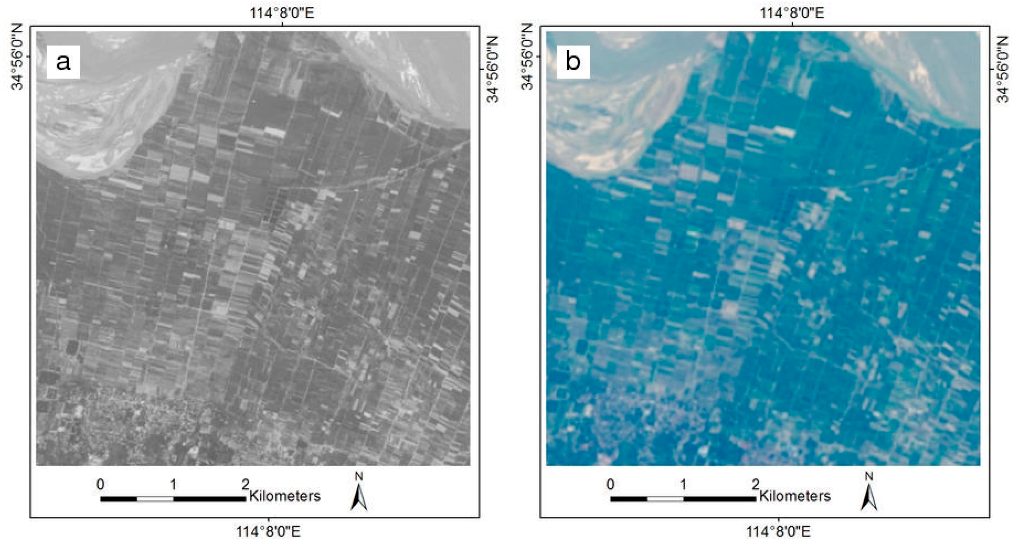
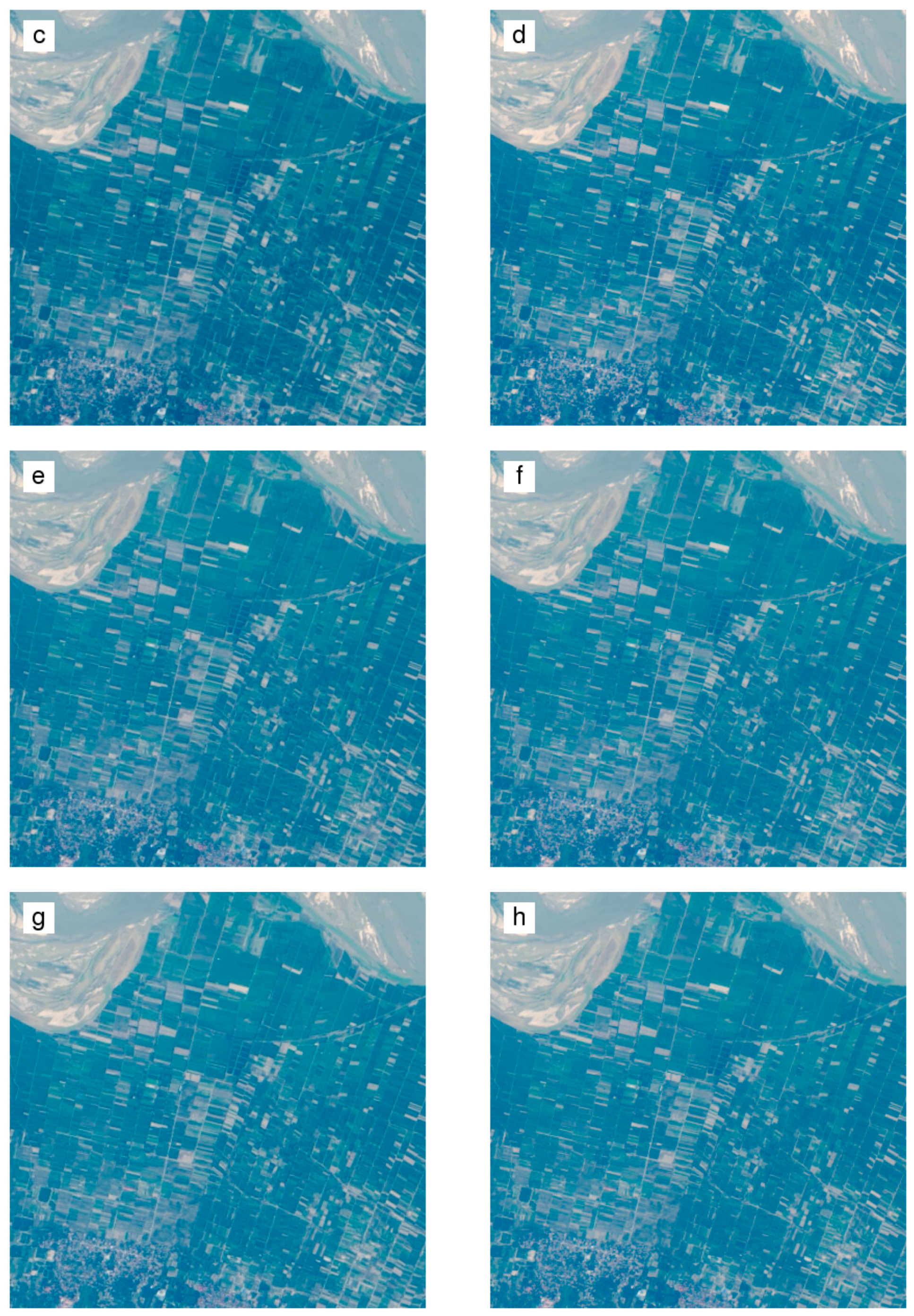
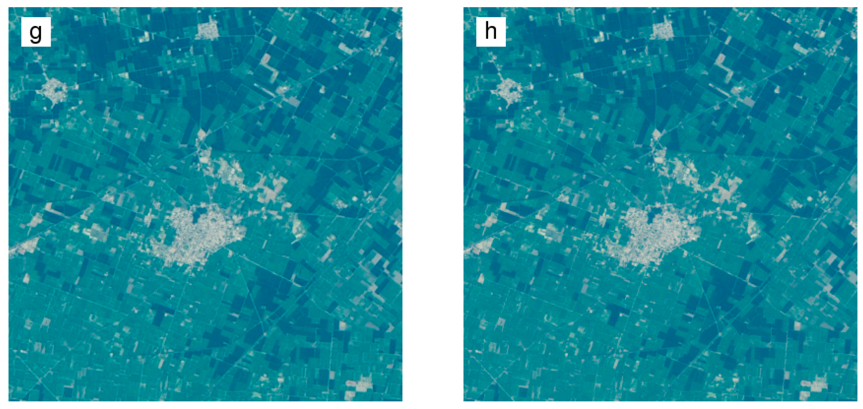
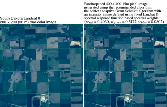
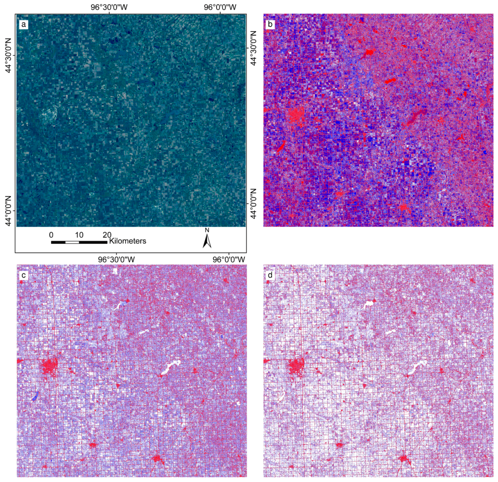
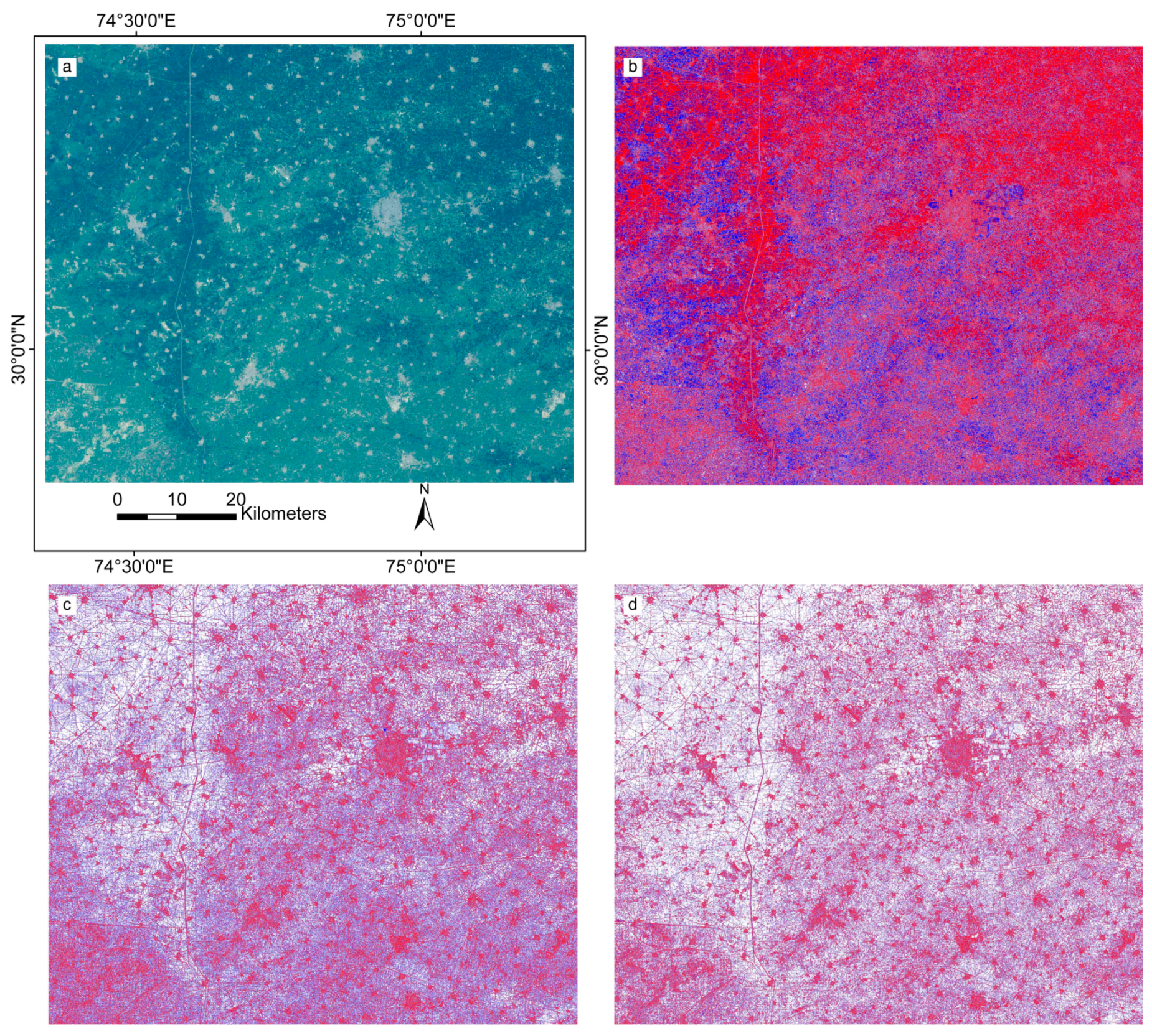
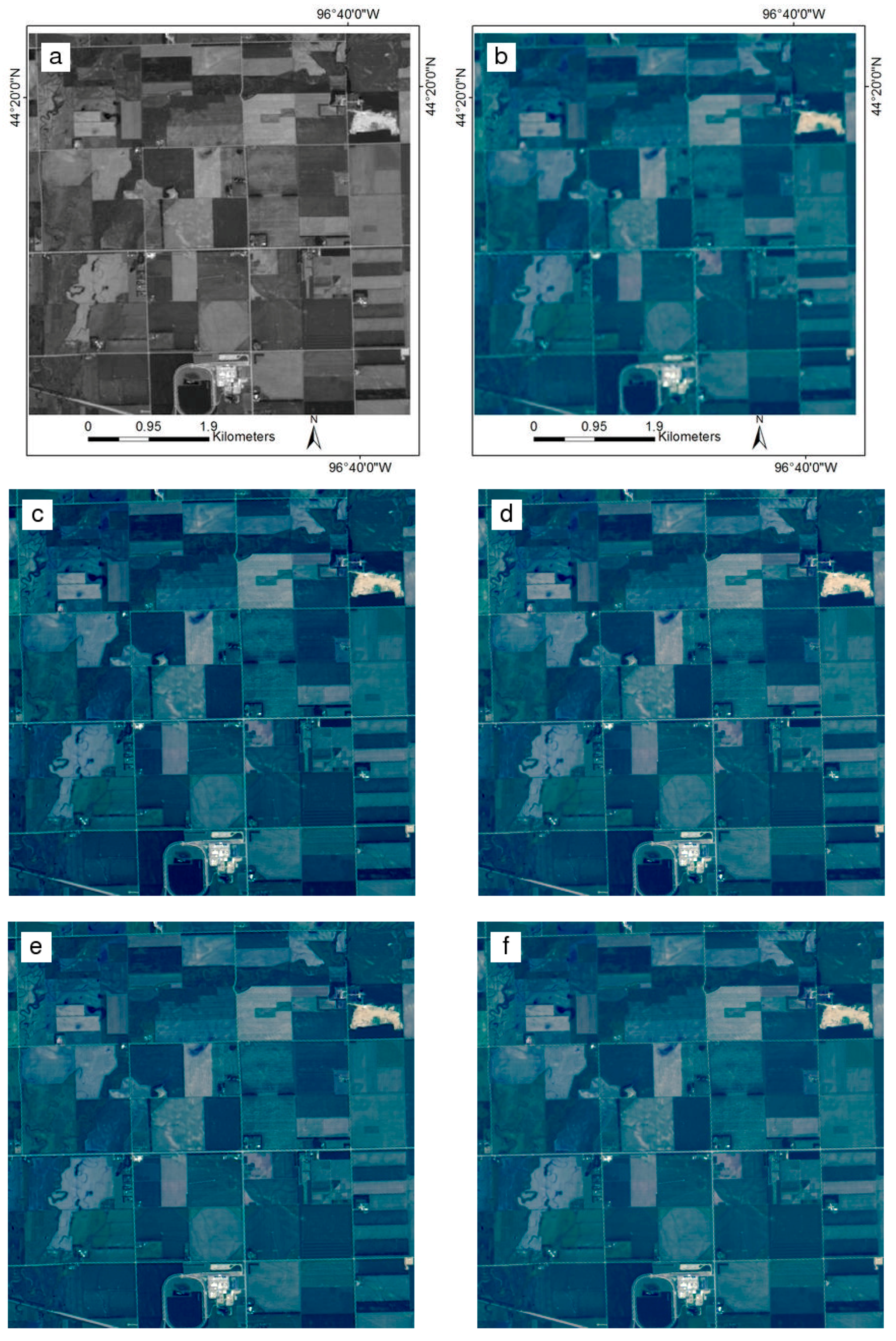
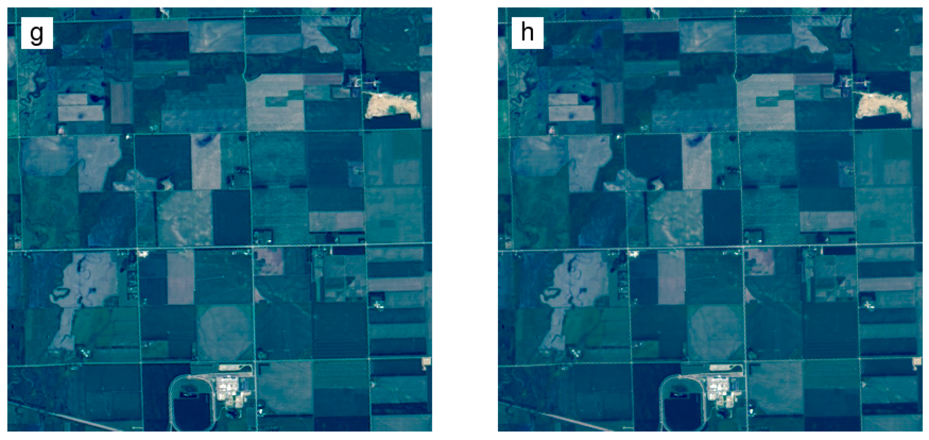
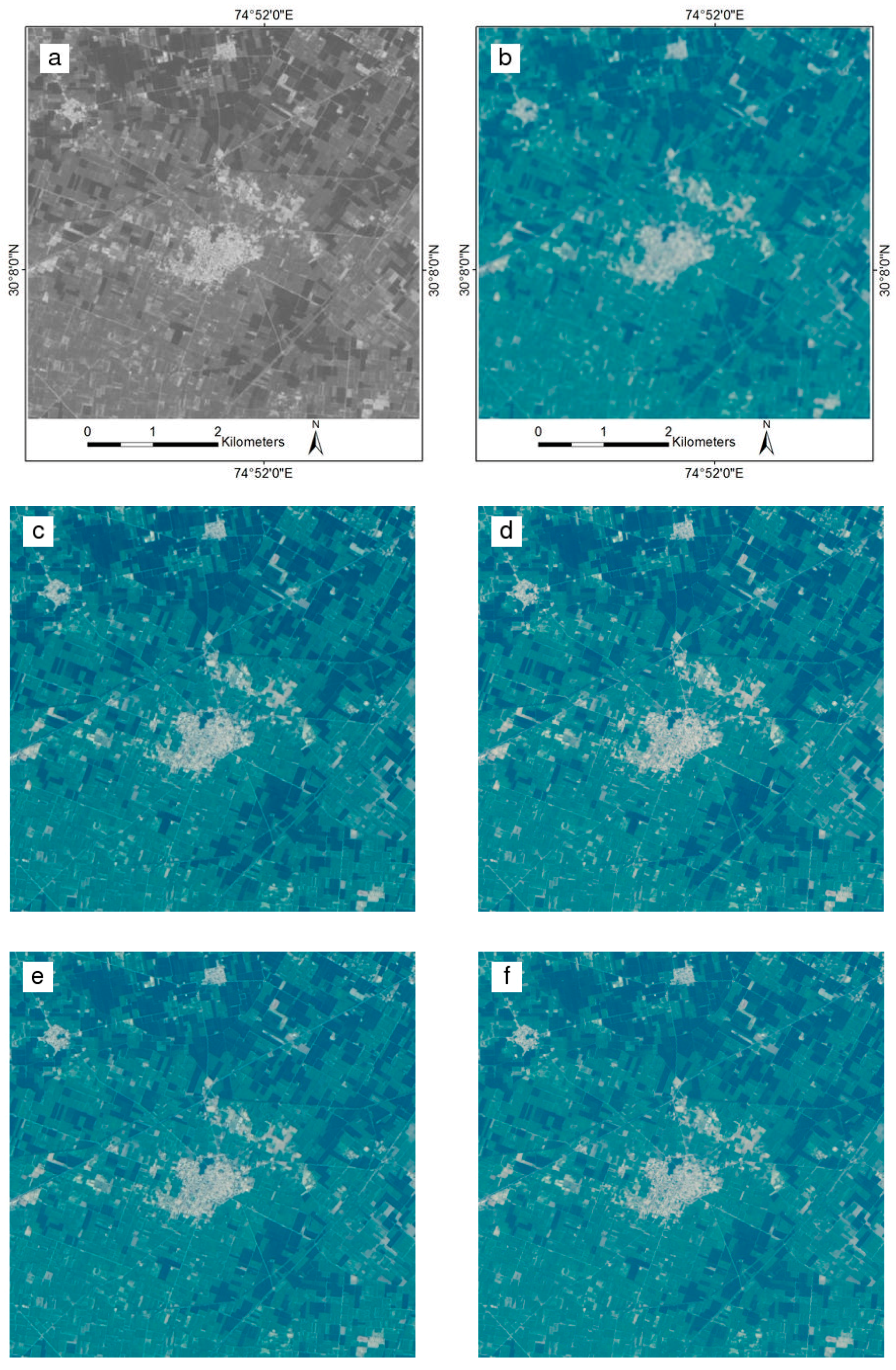
4.3.1. Qualitative Evaluation

Figure 6, Figure 7 and Figure 8 illustrate example pansharpening results for the South Dakota, China and India data respectively. Small 400 × 400 15 m pixel subsets were used to enable detailed visual evaluation. For reference the top figure rows illustrate the 15 m panchromatic (a) and the 30 m true color bands cubic convolution resampled to the panchromatic grid (b). The 15 m Brovey (c,e,g) and context adaptive Gram Schmidt (d,f,h) pansharpening results are shown on the following rows, respectively, with the intensity images derived using equal (c,d), SRFB (e,f), and image specific (g,h) spectral weights. For ease of comparison, the figures are displayed with the same true color and panchromatic contrast stretches.

The pansharpened results (Figure 6, Figure 7 and Figure 8c–h) show more spatial details than the corresponding cubic convolution resampled true color images (b). The pansharpening spatial enhancement is particularly apparent along roads and between crop fields, for example, between the small fields in the China and India subsets (Figure 7 and Figure 8). The distinct South Dakota square 1 × 1 mile road sections (Figure 6) are not quite parallel to the subset image sides, and portions of the road sections are aliased in the cubic convolution resampled true color image while they are not aliased in the pansharpened results. There is, however, no particularly obvious visual difference among the illustrated Brovey and the context adaptive Gram Schmidt pansharpening results. The differences between pansharpened results generated using equal, SRFB, and image specific spectral weights is also subtle, and only clearly discernable for China (Figure 7) where the equal spectral weight results do not correspond spatially with the panchromatic band as well as the SRFB and image specific results.

4.3.2. Quantitative Evaluation

Table 3. Quantitative comparison of the Brovey and context adaptive Gram Schmidt (CA-GS) pansharpening results for the South Dakota (Figure 3), China (Figure 4), and India (Figure 5) red, green, blue and NIR 12 bit images. The ERGAS metric has a zero value when there is no spectral distortion and increasingly positive value with greater distortion. The SAM metric has a zero value when there is no spectral distortion and increasingly positive value with greater distortion. The Q4 index has a value of unity when there is no spatial and spectral distortion and smaller values down to zero with increasing distortion. The evaluation values shown in bold indicate less distortion than the cubic convolution resampled (no-pansharpening) results. The computational algorithm run time (Section 3.4.4) is also shown.

Study Area	Pansharpening Method	ERGAS Value	SAM Value	Q4 Value	Algorithm Run Time (s)
South Dakota 2734 × 2532 30 m pixels	Cubic convolution (no pansharpening)	2.016	1.876	0.902	0.17
	Brovey equal weights	2.669	1.876	0.806	0.76
	Brovey SRFB weights	2.191	1.876	0.815	0.78
	Brovey image specific weights	1.989	1.876	0.819	133.54
	CA-GS equal weights	1.728	1.734	0.918	583.61
	CA-GS SRFB weights	1.513	1.580	0.917	575.05
	CA-GS image specific weights	1.491	1.602	0.916	719.93
China 2976 × 2520 30 m pixels	Cubic convolution (no pansharpening)	1.741	1.731	0.843	0.16
	Brovey equal weights	2.730	1.731	0.758	0.78
	Brovey SRFB weights	1.800	1.731	0.763	0.77
	Brovey image specific weights	1.686	1.731	0.764	142.75
	CA-GS equal weights	1.735	1.786	0.876	621.75
	CA-GS SRFB weights	1.372	1.491	0.876	614.83
	CA-GS image specific weights	1.346	1.461	0.874	756.97
India 2970 × 2470 30 m pixels	Cubic convolution (no pansharpening)	1.543	1.471	0.854	0.15
	Brovey equal weights	2.021	1.471	0.740	0.78
	Brovey SRFB weights	1.608	1.471	0.737	0.77
	Brovey image specific weights	1.499	1.471	0.738	139.93
	CA-GS equal weights	1.377	1.333	0.883	610.39
	CA-GS SRFB weights	1.109	1.151	0.883	605.76
	CA-GS image specific weights	1.093	1.156	0.881	747.57

summarizes for all of each study area the ERGAS, SAM and Q4 pansharpening evaluation metrics applied to the no-pansharpening cubic convolution resampled reflectance as a benchmark, and applied to the Brovey and context adaptive Gram Schmidt (CA-GS) pansharpened reflectance bands derived using the different spectral weights. The three evaluation metrics quantify in different ways the average amount of spectral and spatial distortion in the pansharpened red, green, blue and NIR bands.

The Table 3 evaluation metric values shown in bold denote pansharpened results with less distortion than the no-pansharpening, cubic-convolution resampled results. As expected from the literature [18] the context adaptive Gram Schmidt (CA-GS) pansharpened results have lower distortion, as quantified by the ERGAS, SAM and Q4 measures, than the Brovey results for all the study areas.

Considering the ERGAS spectral distortion metric, only the Brovey equal and SRFB spectral weight results have more spectral distortion than the benchmark cubic convolution resampled data. The spectral distortion quantified by SAM is the same for the Brovey and cubic convolution resampled results because the Brovey modulation coefficients are proportional to the resampled multi-spectral reflectance [23] and thus do not change the SAM (spectral angle) values. The context adaptive Gram Schmidt (CA-GS) pansharpened data have generally less SAM spectral distortion than the benchmark cubic convolution data. The Q4 metric quantifies the degree of spectral and spatial distortion (unlike ERGAS and SAM, greater Q4 metric values indicate less distortion). All the CA-GS pansharpening methods have less spectral and spatial distortion than the cubic convolution resampled data. All the Brovey pansharpening methods have more spectral and spatial distortion than the cubic convolution resampled data.

In all cases (3 study areas and 3 evaluation metrics) the pansharpened results derived using intensity images computed with equal spectral weights have the greatest distortion (or the same distortion as the cubic convolution baseline for the SAM results). This illustrates the utility of knowledge of the sensor spectral response function and the image specific approaches to appropriately parameterize component substitution pansharpening methods. The pansharpened results derived using intensity images computed using the SRFB and the image specific spectral weights are quite comparable. In all cases (3 study areas and 3 metrics) the pansharpened results have less ERGAS measured distortion when computed with the image specific rather than the SRFB spectral weights. However, for the SAM and Q4 distortion measures there is no clear pattern between the SRFB and the image specific spectral weight results.

4.4. Computational Efficiency Evaluation

The benchmark cubic convolution resampling algorithm is computationally the most efficient, with run times of less than 0.2 s for all three study area data sets. The Brovey and then the context adaptive Gram Schmidt (CA-GS) pansharpening algorithm have longer run times respectively. The CA-GS algorithm has the longest run times because of the local neighborhood covariance and variance calculation Equation (9). As expected the run time differences between the equal and SRFB spectral weights is negligible for either the Brovey or CA-GS pansharpening algorithms because the spectral weights are fixed. Compared to the fixed spectral weights the run times for the image specific algorithms are always longer. This is because the image specific algorithm requires two additional operations (degradation of the panchromatic image and image band regression analyses). The Brovey run times are about 200 times longer when image specific rather than fixed (equal and SRFB) spectral weights are used. The CA-GS run times are about one third longer when image specific rather than fixed spectral weights are used. The CA-GS image specific run times are more than five times longer than the Brovey image specific run times.

The pansharpening algorithm computational efficiency becomes important when pansharpening large Landsat image collections. For example, the annual global WELD Landsat data sets available at (http://globalweld.cr.usgs.gov/collections/) were generated considering approximately 140,000 Landsat 5 and 7 images per year. The three test images considered in this study are approximately one fourth the area of a Landsat image. Thus, the computational run time to pansharpen the typical annual global WELD product input data using the Brovey SRFB weights (0.78 s per test image) and the CA-GS SRFB weights (614.9 s per test image) methods would be about 5 and 3985 days respectively. However, the implementation efficiency could be improved greatly by using more efficient programming languages (e.g., compiled languages such as C), using Graphics Processing Unit enhanced computing, and using parallel processing approaches [63].

5. Conclusions

The Landsat 8 satellite has a systematic global image acquisition strategy and precisely coregistered 30 m red, green, blue, NIR and 15 m panchromatic bands [7,14,15]. This study assessed computationally efficient component substitution (CS) pansharpening algorithms suitable for global Landsat 8 data application. There are many algorithms documented in the literature [5,17,53] but CS algorithms are considered to perform similarly to other more computationally expensive algorithms [6,20,21]. CS algorithms first derive a single band intensity image as a weighted linear combination of the multispectral band values. In this study the intensity image was derived using spectral weights defined in three different ways (i) fixed equal spectral weights; (ii) fixed spectral response function based (SRFB) spectral weights derived considering laboratory spectra and the Landsat 8 OLI spectral response functions; and (iii) image specific spectral weights derived using a regression between the multispectral and the degraded panchromatic band [24]. Despite the only minor overlap of the Landsat 8 blue band with the panchromatic band, the SRFB spectral weights found by regressing simulated panchromatic reflectance against simulated red, green and blue reflectance were better fitted than using just simulated red and green reflectance. The novel method to derive the SRFB spectral weights developed in this study for Landsat 8 OLI can be applied to other sensors if the sensor spectral response functions are documented.

In the pansharpening community the tradeoff between minimization of spectral distortion and maximization of spatial contrast is well recognized. In this study we focused on the development and assessment of pansharpening approaches appropriate for scientific data use rather than for visualization purposes. Therefore we placed more emphasis on quantitative evaluation (based on spectral and spatial distortion of the pansharpened results compared to a reference image) than qualitative visual analysis assessment. Two well established CS pansharpening algorithms, Brovey [23] and context adaptive Gram Schmidt [18], were implemented and applied to three predominantly agricultural cloud-free Landsat 8 OLI images. The degree of red, green, blue and NIR pansharpened spectral and spatial distortion was quantified using three established metrics. The context adaptive Gram Schmidt pansharpened results had lower distortion than the Brovey results. The greatest distortion was found when the intensity image was derived using equal spectral weights. Similar levels of distortion were found using the SRFB and image specific spectral weights, with less distortion provided by the image specific spectral weights as quantified by the ERGAS spectral measure. The computational cost (run time) using the image specific weights compared to using the SRFB spectral weights was found to be about 200 and one third times longer for the Brovey and context adaptive Gram Schmidt algorithms respectively. There results indicate that for global Landsat 8 application the context adaptive Gram Schmidt pansharpening algorithm derived using an intensity image defined using the fixed the SRFB spectral weights ($w_{red}$ = 0.4030, $w_{green}$ = 0.5177, and $w_{blue}$ = 0.0802) is appropriate. If computational efficiency is less important than the context adaptive Gram Schmidt pansharpening algorithm derived using an intensity image defined with image specific weights may also be considered. Large area application of Landsat 8 OLI pansharpening is computationally expensive as the 30 m data must be resampled into registration with the 15 m panchromatic band grid. However, if large area Landsat mosaics are generated, for example, as in [9], then this resampling can be undertaken as part of the image to large area map reprojection process. Consequently, further research to demonstrate and assess other advanced pansharpening algorithms using the three band spectral response function based spectral weights, for large area Landsat 8 OLI pansharpened mosaic generation is recommended.

References

1. Wald, L.; Ranchin, T.; Mangolini, M. Fusion of satellite images of different spatial resolutions: Assessing the quality of resulting images. Photogramm. Eng. Remote Sens. 1997, 63, 691–699. [Google Scholar]
2. Pohl, C.; van Genderen, J.L. Multisensor image fusion in remote sensing: Concepts, methods and applications. Int. J. Remote Sens. 1998, 19, 823–854. [Google Scholar] [CrossRef]
3. Tu, T.-M.; Su, S.-C.; Shyu, H.-C.; Huang, P.S. A new look at IHS-like image fusion methods. Inf. Fusion 2001, 2, 177–186. [Google Scholar] [CrossRef]
4. Zhang, Y. Understanding image fusion. Photogramm. Eng. Remote Sens. 2004, 70, 657–661. [Google Scholar]
5. Vivone, G.; Alparone, L.; Chanussot, J.; Dalla Mura, M.; Garzelli, A.; Licciardi, G.A.; Restaino, R.; Wald, L. A critical comparison among pansharpening algorithms. IEEE Trans. Geosci. Remote Sens. 2015, 53, 2565–2586. [Google Scholar] [CrossRef]
6. Garzelli, A. Pansharpening of multispectral images based on nonlocal parameter optimization. IEEE Trans. Geosci. Remote Sens. 2015, 53, 2096–2107. [Google Scholar] [CrossRef]
7. Loveland, T.R.; Dwyer, J.L. Landsat: Building a strong future. Remote Sens Environ. 2012, 122, 22–29. [Google Scholar] [CrossRef]
8. Wulder, M.A.; White, J.C.; Loveland, T.R.; Woodcock, C.E.; Belward, A.S.; Cohen, W.B.; Fosnight, G.; Shaw, J.; Masek, J.G.; Roy, D.P. The global Landsat archive: Status, consolidation, and direction. Remote Sens. Environ. 2016. [Google Scholar] [CrossRef]
9. Roy, D.P.; Ju, J.; Kline, K.; Scaramuzza, P.L.; Kovalskyy, V.; Hansen, M.; Loveland, T.R.; Vermote, E.; Zhang, C. Web-enabled Landsat data (WELD): Landsat ETM+ composited mosaics of the conterminous United States. Remote Sens. Environ. 2010, 114, 35–49. [Google Scholar] [CrossRef]
10. Gong, P.; Wang, J.; Yu, L.; Zhao, Y.; Zhao, Y.; Liang, L.; Niu, Z.; Huang, X.; Fu, H.; Liu, S. Finer resolution observation and monitoring of global land cover: First mapping results with Landsat TM and ETM+ data. Int. J. Remote Sens. 2013, 34, 2607–2654. [Google Scholar] [CrossRef]
11. Hansen, M.C.; Potapov, P.V.; Moore, R.; Hancher, M.; Turubanova, S.; Tyukavina, A.; Thau, D.; Stehman, S.; Goetz, S.; Loveland, T. High-resolution global maps of 21st-century forest cover change. Science 2013, 342, 850–853. [Google Scholar] [CrossRef] [PubMed]
12. Vivone, G.; Simões, M.; Dalla Mura, M.; Restaino, R.; Bioucas-Dias, J.M.; Licciardi, G.A.; Chanussot, J. Pansharpening based on semiblind deconvolution. IEEE Trans. Geosci. Remote Sens. 2015, 53, 1997–2010. [Google Scholar] [CrossRef]
13. Verpoorter, C.; Kutser, T.; Seekell, D.A.; Tranvik, L.J. A global Inventory of lakes based on high-resolution satellite imagery. Geophys. Res. Lett. 2014. 2014GL060641. [Google Scholar]
14. Roy, D.P.; Wulder, M.A.; Loveland, T.R.; Woodcock, C.E.; Allen, R.G.; Anderson, M.C.; Helder, D.; Irons, J.R.; Johnson, D.M.; Kennedy, R.; et al. Landsat-8: Science and product vision for terrestrial global change research. Remote Sens. Environ. 2014, 145, 154–172. [Google Scholar] [CrossRef]
15. Irons, J.R.; Dwyer, J.L.; Barsi, J.A. The next Landsat satellite: The Landsat data continuity mission. Remote Sens. Environ. 2012, 122, 11–21. [Google Scholar] [CrossRef]
16. Ranchin, T.; Wald, L. Fusion of high spatial and spectral resolution images: The ARSIS concept and its implementation. Photogramm. Eng. Remote Sens. 2000, 66, 49–61. [Google Scholar]
17. Thomas, C.; Ranchin, T.; Wald, L.; Chanussot, J. Synthesis of multispectral images to high spatial resolution: A critical review of fusion methods based on remote sensing physics. IEEE Trans. Geosci. Remote Sens. 2008, 46, 1301–1312. [Google Scholar] [CrossRef] [Green Version]
18. Aiazzi, B.; Baronti, S.; Lotti, F.; Selva, M. A comparison between global and context-adaptive pansharpening of multispectral images. IEEE Geosci. Remote Sens. Lett. 2009, 6, 302–306. [Google Scholar] [CrossRef]
19. Zhang, H.K.; Huang, B. A new look at image fusion methods from a bayesian perspective. Remote Sens. 2015, 7, 6828–6861. [Google Scholar] [CrossRef]
20. Baronti, S.; Aiazzi, B.; Selva, M.; Garzelli, A.; Alparone, L. A theoretical analysis of the effects of aliasing and misregistration on pansharpened imagery. IEEE J. Sel. Top. Signal. Process. 2011, 5, 446–453. [Google Scholar] [CrossRef]
21. Xu, Q.; Li, B.; Zhang, Y.; Ding, L. High-fidelity component substitution pansharpening by the fitting of substitution data. IEEE Trans. Geosci. Remote Sens. 2014, 52, 7380–7392. [Google Scholar]
22. Shah, V.P.; Younan, N.H.; King, R.L. An efficient pan-sharpening method via a combined adaptive PCA approach and contourlets. IEEE Trans. Geosci. Remote 2008, 46, 1323–1335. [Google Scholar] [CrossRef]
23. Gillespie, A.R.; Kahle, A.B.; Walker, R.E. Color enhancement of highly correlated images. II. Channel ratio and “chromaticity” transformation techniques. Remote Sens. Environ. 1987, 22, 343–365. [Google Scholar] [CrossRef]
24. Aiazzi, B.; Baronti, S.; Selva, M. Improving component substitution pansharpening through multivariate regression of MS plus Pan data. IEEE Trans. Geosci. Remote Sens. 2007, 45, 3230–3239. [Google Scholar] [CrossRef]
25. Barsi, J.A.; Markham, B.L.; Pedelty, J.A. The operational land imager: spectral response and spectral uniformity. Proc. SPIE 2011. [Google Scholar] [CrossRef]
26. NASA Landsat Science. Spectral Response of the Operational Land Imager In-Band, Band-Average Relative Spectral Response. 2014. Available online: http://landsat.gsfc.nasa.gov/?p=5779 (accessed on 17 September 2014). [Google Scholar]
27. Arvidson, T.; Gasch, J.; Goward, S.N. Landsat 7's long-term acquisition plan—An innovative approach to building a global imagery archive. Remote Sens. Environ. 2001, 78, 13–26. [Google Scholar] [CrossRef]
28. Yan, L.; Roy, D.P. Automated crop field extraction from multi-temporal Web Enabled Landsat Data. Remote Sens. Environ. 2014, 144, 42–64. [Google Scholar] [CrossRef]
29. Fan, S.G.; Chan-Kang, C. Is small beautiful? Farm size, productivity, and poverty in Asian agriculture. Agric. Econ. Blackwell. 2005, 32, 135–146. [Google Scholar] [CrossRef]
30. Long, H.; Zou, J.; Pykett, J.; Li, Y. Analysis of rural transformation development in China since the turn of the new millennium. Appl. Geogr. 2011, 31, 1094–1105. [Google Scholar] [CrossRef]
31. White, E.V.; Roy, D.P. A contemporary decennial examination of changing agricultural field sizes using Landsat time series data. Geo: Geogr. Environ. 2015, 2, 33–54. [Google Scholar] [CrossRef]
32. Kalubarme, A.H.; Potdar, M.B.; Manjunath, K.R.; Mahey, R.K.; Siddhu, S.S. Growth profile based crop yield models: A case study of large area wheat yield modelling and its extendibility using atmospheric corrected NOAA AVHRR data. Int. J. Remote Sens. 2003, 24, 2037–2054. [Google Scholar] [CrossRef]
33. Joint Agricultural Weather Facility, World Agricultural Outlook Board, United States Department of Agriculture. Major World Crop Areas and Climatic Profiles; Agricultural Handbook No. 664; United States Department of Agriculture: Washington, DC, USA, 1992.
34. Chauhan, B.S.; Mahajan, G.; Sardana, V.; Timsina, J.; Jat, M.L. Productivity and sustainability of the rice-wheat cropping system in the Indo-Gangetic Plains of the Indian subcontinent: Problems, opportunities, and strategies. In Advances in Agronomy; Donald, L.S., Ed.; Academic Press: Waltham, MA, USA, 2012; pp. 315–369. [Google Scholar]
35. Clark, R.L.; Swayze, G.A.; Wise, R.; Livo, K.E.; Hoefen, T.; Kokaly, R.F.; Sutley, S.J. USGS Digital Spectral Library splib06a. U.S. Geological Survey, 2007. Available online: http://speclab.cr.usgs.gov/spectral.lib06 (accessed on 19 September 2014). [Google Scholar]
36. Baldridge, A.M.; Hook, S.J.; Grove, C.I.; Rivera, G. The ASTER spectral library version 2.0. Remote Sens. Environ. 2009, 113, 711–715. [Google Scholar] [CrossRef]
37. ENVI. ENVI 5.1 spectral library readme files. Assessed in the installation directory of ENVI 5.1. 2013. [Google Scholar]
38. Ju, J.; Roy, D.P.; Vermote, E.; Masek, J.; Kovalskyy, V. Continental-scale validation of MODIS-based and LEDAPS Landsat ETM+ atmospheric correction methods. Remote Sens. Environ. 2012, 122, 175–184. [Google Scholar] [CrossRef]
39. Roy, D.P.; Qin, Y.; Kovalskyy, V.; Vermote, E.F.; Ju, J.; Egorov, A.; Hansen, M.C.; Kommareddy, I.; Yan, L. Conterminous United States demonstration and characterization of MODIS-based Landsat ETM+ atmospheric correction. Remote Sens Environ. 2014, 140, 433–449. [Google Scholar] [CrossRef]
40. Steven, M.D.; Malthus, T.J.; Baret, F.; Xu, H.; Chopping, M.J. Intercalibration of vegetation indices from different sensor systems. Remote Sens. Environ. 2003, 88, 412–422. [Google Scholar] [CrossRef]
41. Ouaidrari, H.; Vermote, E.F. Operational atmospheric correction of Landsat TM data. Remote Sens. Environ. 1999, 70, 4–15. [Google Scholar] [CrossRef]
42. Reichenbach, S.E.; Koehler, D.E.; Strelow, D.W. Restoration and reconstruction of AVHRR images. IEEE Trans. Geosci. Remote Sens. 1995, 33, 997–1007. [Google Scholar] [CrossRef]
43. Roy, D.P. The impact of misregistration upon composited wide field of view satellite data and implications for change detection. IEEE Trans. Geosci. Remote Sens. 2000, 38, 2017–2032. [Google Scholar] [CrossRef]
44. Tanre, D.; Herman, M.; Deschamps, P. Influence of the background contribution upon space measurements of ground reflectance. Appl. Opt. 1981, 20, 3676–3684. [Google Scholar] [CrossRef] [PubMed]
45. Aiazzi, B.; Alparone, L.; Baronti, S.; Garzelli, A.; Selva, M. MTF-tailored multiscale fusion of high-resolution MS and pan imagery. Photogramm. Eng. Remote Sens. 2006, 72, 591–596. [Google Scholar] [CrossRef]
46. Shlien, S. Geometric correction, registration and resampling of Landsat imagery. Can. J. Remote Sens. 1979, 5, 75–89. [Google Scholar] [CrossRef]
47. Park, S.K.; Schowengerdt, R.A. Image reconstruction by parametric cubic convolution. Comput. Vis. Gr. Image Process. 1983, 23, 258–272. [Google Scholar] [CrossRef]
48. Keys, R. Cubic convolution interpolation for digital image processing. IEEE Trans. Acoust. Speech Signal. Process. 1981, 29, 1153–1160. [Google Scholar] [CrossRef]
49. Dikshit, O.; Roy, D.P. An empirical investigation of image resampling effects upon the spectral and textural supervised classification of a high spatial resolution multispectral image. Photogramm. Eng. Remote Sens. 1996, 62, 1085–1092. [Google Scholar]
50. Aiazzi, B.; Baronti, S.; Selva, M.; Alparone, L. Bi-cubic interpolation for shift-free pan-sharpening. ISPRS J. Photogramm. Remote Sens. 2013, 86, 65–76. [Google Scholar] [CrossRef]
51. Kalpoma, K.A.; Kawano, K.; Kudoh, J. IKONOS image fusion process using steepest descent method with bi-linear interpolation. Int. J. Remote Sens. 2013, 34, 505–518. [Google Scholar] [CrossRef]
52. Laben, C.A.; Brower, B.V. Process for Enhancing the Spatial Resolution of Multispectral Imagery Using Pan-Sharpening. U.S. Patent 6,011,875, 2000. [Google Scholar]
53. Alparone, L.; Wald, L.; Chanussot, J.; Thomas, C.; Gamba, P.; Bruce, L.M. Comparison of pansharpening algorithms: Outcome of the 2006 GRS-S data-fusion contest. IEEE Trans. Geosci. Remote Sens. 2007, 45, 3012–3021. [Google Scholar] [CrossRef] [Green Version]
54. Alparone, L.; Baronti, S.; Garzelli, A.; Nencini, F. A global quality measurement of pan-sharpened multispectral imagery. IEEE Geosci. Remote Sens. Lett. 2004, 1, 313–317. [Google Scholar] [CrossRef]
55. Kruse, F.A.; Lefkoff, A.B.; Boardman, J.W.; Heidebrecht, K.B.; Shapiro, A.T.; Barloon, P.J.; Goetz, A.F.H. The spectral image-processing system (SIPS)—interactive visualization and analysis of imaging spectrometer data. Remote Sens. Environ. 1993, 44, 145–163. [Google Scholar] [CrossRef]
56. Keshava, N. Distance metrics and band selection in hyperspectral processing with applications to material identification and spectral libraries. IEEE Transs. Geosci. Remote Sens. 2004, 42, 1552–1565. [Google Scholar] [CrossRef]
57. Wald, L. Data Fusion: Definitions and Architectures—Fusion of Images of Different Spatial Resolutions; Les Presses: Paris, France, 2002. [Google Scholar]
58. Wang, Z.; Bovik, A.C. A universal image quality index. IEEE Signal. Process. Lett. 2002, 9, 81–84. [Google Scholar] [CrossRef]
59. Painter, T.H.; Rittger, K.; McKenzie, C.; Slaughter, P.; Davis, R.E.; Dozier, J. Retrieval of subpixel snow covered area, grain size, and albedo from MODIS. Remote Sens. Environ. 2009, 113, 868–879. [Google Scholar] [CrossRef]
60. Ustin, S.L.; Roberts, D.A.; Pinzón, J.; Jacquemoud, S.; Gardner, M.; Scheer, G.; Castañeda, C.M.; Palacios-Orueta, A. Estimating canopy water content of chaparral shrubs using optical methods. Remote Sens. Environ. 1998, 65, 280–291. [Google Scholar] [CrossRef]
61. Czapla-Myers, J.S.; Anderson, N.J.; Biggar, S.F. Early ground-based vicarious calibration results for Landsat 8 OLI. Proc. SPIE 2013. [Google Scholar] [CrossRef]
62. Markham, B.L.; Storey, J.C.; Irons, J.R. Landsat data continuity mission, now Landsat-8: Six months on-orbit. Proc. SPIE 2013. [Google Scholar] [CrossRef]
63. Yang, J.; Zhang, J.; Huang, G. A parallel computing paradigm for pan-sharpening algorithms of remotely sensed images on a multi-core computer. Remote Sens. 2014, 6, 6039–6063. [Google Scholar] [CrossRef]
Figure 1. Landsat 8 spectral response functions for the blue, green, red, panchromatic (black) and near-infrared (NIR) (dark orange) bands.
Remotesensing 08 00180 g001
Figure 2. Example vegetation, soil, water and snow spectra and the simulated (see Equation (3)) panchromatic (black asterisk), red (red dot), green (green dot), and blue (blue dot) Landsat 8 Operational Land Imager (OLI) reflectance plotted at the Landsat 8 band center wavelengths.
Remotesensing 08 00180 g002
Figure 3. South Dakota 2734 × 2532 30 m Landsat 8 top of atmosphere (TOA) red, green, blue TOA reflectance (a). Absolute reflectance differences between the 15m panchromatic band and the 15 m resampled intensity images generated using: the equal spectral weights ( w r e d = w g r e e n = w b l u e = ⅓) (b); the spectral response function based (SRFB) spectral weights ( w r e d = 0.4030, w g r e e n = 0.5177, w b l u e = 0.0802) (c); and the image specific spectral weights ( w r e d = 0.4516, w g r e e n = 0.5981, w b l u e = −0.0588) (d). Absolute reflectance differences colored as: 0 ≤ white < 0.0035, 0.0035 ≤ blue < 0.0070, and red ≥ 0.0070. The 30 m true color and the 30 m intensity images were cubic convolution resampled to the 15 m panchromatic band grid.
Remotesensing 08 00180 g003
Figure 4. China 2976 × 2520 30 m Landsat 8 TOA red, green, blue TOA reflectance (a). Absolute reflectance differences between the 15 m panchromatic band and the 15 m resampled intensity images generated using: the equal spectral weights ( w r e d = w g r e e n = w b l u e = ⅓) (b); the spectral response function based (SRFB) spectral weights ( w r e d = 0.4030, w g r e e n = 0.5177, w b l u e = 0.0802) (c); and the image specific spectral weights ( w r e d = 0.4568, w g r e e n = 0.5041, w b l u e = 0.0361) (d). Absolute reflectance differences colored as: 0 ≤ white < 0.0035, 0.0035 ≤ blue < 0.0070, and red ≥ 0.0070. The 30 m true color and the 30 m intensity images were cubic convolution resampled to the 15 m panchromatic band grid.
Remotesensing 08 00180 g004
Figure 5. India 2970 × 2470 30 m Landsat 8 TOA red, green, blue TOA reflectance (a). Absolute reflectance differences between the 15 m panchromatic band and the 15 m resampled intensity images generated using: the equal spectral weights ( w r e d = w g r e e n = w b l u e = ⅓) (b); the spectral response function based (SRFB) spectral weights ( w r e d = 0.4030, w g r e e n = 0.5177, w b l u e = 0.0802) (c); and the image specific spectral weights w r e d = 0.4922, w g r e e n = 0.4586, w b l u e = 0.0512) (d). Absolute reflectance differences colored as: 0 ≤ white < 0.0035, 0.0035 ≤ blue < 0.0070, and red ≥ 0.0070. The 30 m true color and the 30 m intensity images were cubic convolution resampled to the 15m panchromatic band grid.
Remotesensing 08 00180 g005
Figure 6. South Dakota illustrative 400 × 400 (15 m) pixel subset. Top row: 15 m TOA panchromatic reflectance (a) and 30 m true color (red, green and blue) TOA reflectance cubic convolution resampled to 15 m (b); The following rows show 15 m true color Brovey (left column) and context adaptive Gramm-Schmidt (right column) pansharpened reflectance respectively, derived using intensity images computed using the equal (c,d); spectral response function based (SRFB) (e,f); and image specific spectral weights (g,h) summarized in the Figure 3 caption.
Remotesensing 08 00180 g006aRemotesensing 08 00180 g006b
Figure 7. China illustrative 400 × 400 (15 m) subset. Top row: 15 m TOA panchromatic reflectance (a) and 30 m true color (red, green and blue) TOA reflectance cubic convolution resampled to 15 m (b); The following rows show 15 m true color Brovey (left column) and context adaptive Gramm-Schmidt (right column) pansharpened reflectance respectively, derived using intensity images computed using the equal (c,d); spectral response function based (SRFB) (e,f); and image specific spectral weights (g,h) summarized in the Figure 4 caption.
Remotesensing 08 00180 g007aRemotesensing 08 00180 g007b
Figure 8. India illustrative 400 × 400 (15 m) subset. Top row: 15 m TOA panchromatic reflectance (a) and 30 m true color (red, green and blue) TOA reflectance cubic convolution resampled to 15 m (b); The following rows show 15 m true color Brovey (left column) and context adaptive Gramm-Schmidt (right column) pansharpened reflectance respectively, derived using intensity images computed using the equal (c,d); spectral response function based (SRFB) (e,f); and image specific spectral weights (g,h) summarized in the Figure 5 caption.
Remotesensing 08 00180 g008aRemotesensing 08 00180 g008b