Article

New Automated Method to Develop Geometrically Corrected Time Series of Brightness Temperatures from Historical AVHRR LAC Data

1
Department of Biodiversity and Molecular Ecology, Research and Innovation Centre, Fondazione Edmund Mach, Trento 38010, Italy
2
Department of Sustainable Agro-Ecosystems and Bioresources, Research and Innovation Centre, Fondazione Edmund Mach, Trento 38010, Italy
3
Department of Biology, Chemistry and Pharmacy, Freie Universität Berlin, Berlin 14195, Germany
4
Swedish Meteorological and Hydrological Institute (SMHI), Norrköping 60176, Sweden
5
Leibniz Institute of Freshwater Ecology and Inland Fisheries (IGB), Berlin 12587, Germany
6
Mundialis GmbH & Co. KG, Bonn 53227, Germany
*
Author to whom correspondence should be addressed.
Remote Sens. 2016, 8(3), 169; https://doi.org/10.3390/rs8030169
Submission received: 31 October 2015 / Revised: 20 January 2016 / Accepted: 4 February 2016 / Published: 25 February 2016

Abstract

:
Analyzing temporal series of satellite data for regional scale studies demand high accuracy in calibration and precise geo-rectification at higher spatial resolution. The Advanced Very High Resolution Radiometer (AVHRR) sensor aboard the National Oceanic and Atmospheric Administration (NOAA) series of satellites provide daily observations for the last 30 years at a nominal resolution of 1.1 km at nadir. However, complexities due to on-board malfunctions and orbital drifts with the earlier missions hinder the usage of these images at their original resolution. In this study, we developed a new method using multiple open source tools which can read level 1B radiances, apply solar and thermal calibration to the channels, remove bow-tie effects on wider zenith angles, correct for clock drifts on earlier images and perform precise geo-rectification by automated generation and filtering of ground control points using a feature matching technique. The entire workflow is reproducible and extendable to any other geographical location. We developed a time series of brightness temperature maps from AVHRR local area coverage images covering the sub alpine lakes of Northern Italy at 1 km resolution (1986–2014; 28 years). For the validation of derived brightness temperatures, we extracted Lake Surface Water Temperature (LSWT) for Lake Garda in Northern Italy and performed inter-platform (NOAA-x vs. NOAA-y) and cross-platform (NOAA-x vs. MODIS/ATSR/AATSR) comparisons. The MAE calculated over available same day observations between the pairs—NOAA-12/14, NOAA-17/18 and NOAA-18/19 are 1.18 K, 0.67 K, 0.35 K, respectively. Similarly, for cross-platform pairs, the MAE varied between 0.5 to 1.5 K. The validation of LSWT from various NOAA instruments with in-situ data shows high accuracy with mean R2 and RMSE of 0.97 and 0.91 K respectively.

Graphical Abstract

1. Introduction

The AVHRR Local Area Coverage (LAC) data which are available at nominal 1.1 km spatial resolution (hereafter AVHRR LAC) with an extensive coverage of the earth is an unique source of the longest medium resolution time series satellite data for regional studies. However, the number of studies which use older AVHRR LAC data are limited, owing to the complexity in achieving acceptable accuracy due to well documented orbital drifts and clock errors with the instruments [1,2,3,4,5]. The archived AVHRR LAC data [6] is stored in 10 bit precision and consist of sensor data in raw digital counts, calibration coefficients, time codes, quality indicators, angles, telemetry etc., which are appended at different bit locations [7]. The data are provided in NOAA level 1B raw format where earth location and calibration parameters are appended with the sensor data (digital numbers) but not applied [8]. The data are freely available on the Comprehensive Large Array-data Stewardship System (CLASS) [6]. CLASS is NOAA’s online facility to distribute data from multiple satellites. Indeed, it requires high level processing taking care of inter-satellite calibrations, multiple versions of AVHRR sensor and correcting for the known issues with the older data [3,8,9,10]. Developing a long term time series combining AVHRR LAC data from multiple NOAA instruments demand two different approaches, one for the POD (Polar Orbiter Data) series of instruments (NOAA-9/11/12/14) and another for the KLM (KLM represents the instrument codes) series (NOAA-16/17/18/19) due to: (i) significant differences in the headers of the POD and KLM series data [8,10]; (ii) varying spectral characteristics of the different versions of the AVHRR sensor—AVHRR/1 and AVHRR/2 for POD and AVHRR/3 for KLM (Table 1); and (iii) pre-processing steps depending upon the corrections to be applied for accurate navigation [3].
The POD instruments suffered largely with position errors due to the orbital drifts, and navigational errors due to discrepancies with the satellite orientation (generally termed as satellite attitude) and satellite clock [1,3]. The satellite position error that occurred from the orbital drift of the instruments, is due to the lack of orbit adjustment systems [2]. This caused a change in the equatorial crossing time from the original (by hours) and the shift often increased with the age of the instrument [11] (Figure 1). In Figure 1, the observation time is plotted for all the NOAA instruments used in this study, showing a rather larger shift with the earlier missions. The effects of orbital drift on the derived vegetation indices and sea surface temperature is well documented by [2,12]. On the other hand, the clock error is due to drift in the satellite clock over time. To overcome this, a periodical reset of the clock was performed in the earlier NOAA instruments [3]. This also contributed to the navigational error due to clock mis-synchronization. To correct the navigational errors, historical ephemeris (position of satellite in space at a given day and time) data stored in two line element format are widely used [3,13]. The attitude control system comprises of three rotation angles - roll, pitch and yaw which control the actual orientation by maintaining the spacecraft fixed axes along the desired geodetic directions [14]. In the earlier AVHRR LAC data attitude errors are difficult to correct due to missing data of roll, pitch and yaw angles. To correct the navigational errors due to attitudinal shifts, the angles are modeled from a set of known landmarks identified from the images, but this approach has limited success [3,14]. The KLM instruments on the other hand were launched with much improved AVHRR/3 six channel sensor and had advanced systems on-board to minimize the navigational errors.
Numerous studies in the past deal with the accurate geolocation of the AVHRR LAC data to develop continuous time series irrespective of the NOAA instrument [1,14,15,16,17,18,19,20,21]. One of the earlier methods is the automatic adjustment of the AVHRR images by applying a physical deformation model of the actual image using the ephemeral elements followed by landmark adjustment using reference Ground Control Points (GCP) along coastal lines [1,15]. With this method an accuracy within one pixel is achieved on images acquired from NOAA-11/12/14. Hüsler, et al. [20] used this method as part of their AVHRR archiving process for images over Europe. Moreno, et al. [17] used a small sample of GCP’s to refine the orbital elements of the satellite thereby improving the registration accuracy of the images. More recently, advanced image matching techniques have been used to extract GCP’s to achieve sub-pixel accuracy in geo-rectification of AVHRR images [18,19]. Latifovic, et al. [18] developed historical AVHRR 1.1 km baseline data over entire Canada and used all the AVHRR LAC data acquired by NOAA POD and KLM instruments. They used an image matching procedure to automatically extract GCP’s.
However, the potential use of earlier AVHRR LAC images is often hindered by lack of a complete solution to accurately process them [14]. They are seldom used in research due to lack of open software tools which can perform the aforementioned corrections and accurately process the data. The available solutions are either outdated, they offer limited success, or are published with proprietary licenses. Newer methods and geospatial libraries have become available in the last decade and it is now worthwhile to revisit the AVHRR navigation [22,23]. At present the ability to accurately process all the AVHRR LAC images are limited to very few research centers with satellite receiving stations. There is also lack of publicly available processed AVHRR LAC dataset covering a particular area of interest; on the other hand, the level 1B data are freely available for any part of the world. Therefore, we see a strong demand for an open source solution to process the AVHRR LAC data in level 1B format for any area of interest which will support the scientists in regional level studies.
Our aim is to develop an automated workflow using multiple open source geospatial libraries and software packages to process all existing AVHRR LAC data (since 1986) for our study area. As a proof of concept, geo-rectified time series (1986–2014) of brightness temperature from the two thermal bands (channels 4 and 5) of AVHRR are developed, which is then intended to be used for estimating the historical surface temperature of sub-alpine lakes [21]. The quality of the developed time series is validated for the automatic geo-rectification and thermal calibration. We estimated long-term LSWT of Lake Garda from the time series of brightness temperatures and performed inter-platform and cross-platform comparisons along with in-situ data to validate the product. We used Pytroll, a set of open source Python libraries originally meant for processing weather satellite data to read, correct and calibrate the AVHRR data [24]. We extended the Pytroll to enhance its support for POD and KLM series of AVHRR LAC data. We used the feature matching technique in Orfeo toolbox for precise geo-rectification [25]. Finally all the post processing including cloud masking, workflow automation, and time series development were accomplished in the GRASS GIS 7.0 software ([23,26,27].

2. Methods

2.1. Data and Software

We obtained all the available AVHRR LAC data from the NOAA public archive (CLASS—[6]) in the period 1986–2014 covering the study area of Northern Italy (Longitude: 42.9762°E–46.2371°E; Latitude: 8.2127°N–12.3456°N; Area: 360 km × 340 km). Only day time images acquired between 8:00 to 17:00 UTC are considered for this study. The data are stored in binary format and consist of two major parts—data header and the scan line data. The data header contains generic data on the instrument, acquisition time, data quality, orbital parameters, and conversion factors for calibration and telemetry data, while the scan line data contain data specific to a single scan or time segment including calibration, navigation, telemetry and sensor data, among many others. A complete list of headers is given here: POD—[10]; KLM—[8]. There are 2048 points in a LAC scan line on which the solar zenith angle and earth location data (latitude and longitude) are sampled at every 40th sample, while the sensor data are recorded for each of the 2048 samples.
Figure 2a,b shows the year-wise distribution of the obtained level 1B data and the time line of all the NOAA instruments, respectively. As listed in the Table 1, AVHRR/1 lacks dual thermal bands required for the split window technique of surface temperature calculation, which is our main goal in processing this data. Hence the AVHRR LAC images acquired by the earliest NOAA instruments—TIROS-N, NOAA-6/8/10 were avoided. Due to non-availability of day images over the study area, data from NOAA-15 were also discarded. In line with the main objective of estimating day time Lake Surface Water Temperature (LSWT) for the sub-alpine lakes in the study area, we processed only the day images.
We combined multiple open source geospatial software packages in a single workflow to meet the specific requirements of AVHRR processing. The software used, its source code links and the licenses are listed in Table 2. Pytroll is an open source project, contributed by several developers primarily from national meteorological services [24]. Among the Pytroll libraries, mpop, pygac and pyresample are used respectively for reading, calibrating, and resampling the AVHRR LAC images. Figure 3 shows their specific roles in the workflow. We used these libraries to read all the AVHRR LAC level 1B data, apply corrections, calibrate and write all the channels to separate TIF images. Orfeo toolbox is a remote sensing image processing toolbox developed in C++ primarily by the Centre National d’Études Spatiales, France [25]. We used the Scale Invariant Feature Transform (SIFT) feature matching algorithm in Orfeo toolbox to extract homologous points (hereafter GCP’s; homologous meaning same relative position, a term used in Orfeo toolbox module – otbcli_HomologousPointsExtraction – for extracting similar GCP’s from two images using feature matching algorithms like SIFT) in order to apply final matching of each image against a reference image [28]. The GCP’s created are then filtered using the newly developed m.gcp.filter tool in GRASS GIS [29]. GRASS GIS is one of the most stable and well established open source geographical information systems and remote sensing software which can handle both vector and raster processing in two and three dimensions [23]. The calibrated AVHRR LAC images are rectified using the filtered GCP’s with i.rectify module in GRASS GIS. We developed all the raster processing and the cloud removal procedure in GRASS GIS [27].
Figure 3 shows the workflow diagram with the respective libraries listed horizontally against the specific requirement they meet.

2.2. Pre-Processing

The pre-processing of AVHRR LAC data in level 1B format include reading the data, performing solar and thermal calibration to the respective channels, applying clock drift correction and cloud removal. The foremost requirement of this methodology was to develop an AVHRR LAC data reader which can read all the versions of AVHRR LAC level 1B data irrespective of the NOAA instrument. The Python library pygac in the Pytroll framework is developed to read and calibrate AVHRR global area coverage level 1B data of 4 km spatial resolution which is derived from LAC data by resampling at every 5th sample along a scanline. We enhanced the pygac library to add support to AVHRR LAC data (Figure 3). The fundamental structure of the AVHRR LAC level 1B header and sensor data records is consistent across data types, however there are significant differences between records originating from various instruments (POD vs. KLM) which have to be dealt separately. Hence we developed and added two readers (lac_pod—POD data and lac_klm—KLM data) in pygac to successfully read and calibrate the AVHRR LAC data irrespective of the NOAA instrument. The newly developed readers are released to the public in the source code repository here-[30]. The main difference between the POD and KLM drivers is the mapping of the header structure. All the different releases of level 1B data types by NOAA over POD are mapped in the new readers following the NOAA documentation (For a complete list of headers refer to: POD—[10]; KLM—[8]). The Python library mpop in the Pytroll framework can read multiple satellite data in raw format and use the coefficients given in the header to apply calibration and corrections [31]. mpop has an extendable objective design which enables us to write plugins to support additional data formats. We developed a plugin (lac_l1b) which is a wrapper to the new LAC readers in pygac to read and calibrate the AVHRR LAC data.
For the calibration of the solar channels (0.63 μm and 0.86 μm) we used the inter-sensor consistent calibration coefficients developed by [32] which ensures the continuity of data even with the transition of satellites. Unlike the solar channels, an on-board calibration is performed on the thermal channels [8,10]. In spite of this, the data are prone to contamination (leading to bias of more than 1 K) with unwanted fluctuations due to multiple factors including; (i) atmospheric attenuation of the signal; (ii) decaying of the instruments; and (iii) solar contamination [9,33]. To remove these perturbations in the true signal [34] introduced a robust median based approach to remove short time fluctuations from a given sample of calibration elements followed by Fourier transform filtering to remove the persisting errors over long time. For more details on thermal calibration, refer to [9] and [34]. The aforementioned calibration techniques are successfully implemented in operation for generating historical AVHRR baseline data records over Canada by [18] and more recently to develop LSWT time series for Alpine lakes in Europe by [21]. In Pytroll, pygac library has implemented thermal calibration procedure as per [8,10] followed by a Fourier transform filtering to remove high frequency fluctuations [34]; which we used to successfully calibrate the thermal channels (Figure 3). The ancillary data like GCP’s and the viewing zenith angle are provided as tie points (51 per scanline). We used pygac library to apply linear interpolation on latitude, longitude and viewing zenith angle tie points to all the points in the geographical grid covered by the data (Figure 3).
The polar orbiting NOAA satellites are launched in sun synchronous orbits at an altitude of around 870 km above Earth [7]. They are designed to acquire two daily snapshots of Earth, one in ascending and other in the descending mode. This is possible due to the wider scan angles (also called zenith angles) of ±55.4° covering approximately a 2300 km wide scene. Subsequently, the spatial resolution also varies significantly off-nadir from 1.1 km at nadir to 4 km at the edges both in along-scan and along-track directions [7]. Due to this wide off-nadir field of view, panoramic bow-tie effects are seen towards the edges of the images (Figure 4a) [35]. This creates artifacts when applying re-projection with nearest-neighbour resampling on the level 1B data. In this methodology, we used an algorithm based on 2D gradient search in the latitude and longitude geolocation fields using their local gradients to project level 1B data to Lambert Azimuth equal-area projection, which corrects for the bow-tie effects. Complete details of the algorithm and its implementation is explained in [35]. In Pytroll, this method is implemented in pyresample library which is used to resample all the AVHRR level 1B data (Figure 3).
The POD satellites (NOAA-9/11/14) were affected by drifts in the satellite clock which in turn contributed to the position errors [3]. The difference between satellite clock time and the actual coordinated universal time (offset Δt) was provided by NOAA periodically (see Section 2 at [10]). The clock drift leads to location error upto 4 km, as the GCP’s are estimated based on the satellite clock [10]. The known offsets Δt for the satellites NOAA-9/11/14 are used in the pygac library to correct for clock drifts.
Unlike for level 2 MODIS products, there are no existing cloud mask available for the level 1B AVHRR LAC data. For this, we adapted the algorithm developed by [36], Separation of Pixels Using Aggregated Rating over Canada (SPARC) originally implemented for creating a cloud mask over Canada. As our main interest is to remove thick clouds and thin cirrus above the lakes, we used two relevant tests from the original SPARC algorithm, (i) Brightness temperature test (T-test) using channel 4 and (ii) thin cirrus test (C-test) which uses the difference between channels 4 and 5. T-test uses the channel 4 brightness temperature and compares it with a dynamic threshold which is the surface skin temperature data of the corresponding day and time derived from climatic models. In the original study, North American regional reanalysis is used. Here we replaced it with the European regional analysis interim dataset developed by the European Center for Medium-range Weather Forecasts(ECMWF) [37] following the successful implementation over Europe by [21]. The SPARC algorithm is implemented using raster processing tools in GRASS GIS 7.0 (Figure 3).

2.3. Precise Geo-Rectification Using SIFT

After calibration and corrections, the AVHRR LAC data still suffer from position errors due to erroneous satellite attitude angles [1,3,14]. For any long-term analysis of landscape properties using historical AVHRR data, it is important to obtain precise geometric position for all the images to avoid spurious trends and artifacts. Hence we used an automatic feature matching technique called Scale Invariant Feature Transform (SIFT) by [28] to extract matching GCP’s between an image pair to achieve sub-pixel accuracy in image to image rectification [18,19]. We selected a cloud-free geometrically corrected image from NOAA-19 ascending mode (dated 1 August 2012) as reference image to all the other data to which image to image matching is applied. The homologous points extraction module in the Orfeo Toolbox 4.4.0 is used to automatically extract the matching GCP’s using the SIFT algorithm (Figure 3). The SIFT algorithm is widely used in object recognition from images [38,39,40] successfully implemented SIFT features in registering multiple source remote sensing imageries. The SIFT workflow starts with identifying and populating the SIFT features from the input and reference images. The SIFT features are scale invariant and highly distinctive which makes them suitable for image matching techniques. The matching SIFT features are then identified based on euclidean distance of their feature vectors. The SIFT algorithm was developed and explained in detail by [28].
We applied SIFT individually to all the bands of a single AVHRR LAC image and combined all the extracted GCP’s. If the total number of matching GCP pairs are less than 20, often due to wide coverage of cloud, then the input image is discarded from further processing. Before applying image rectification using the extracted GCP’s, it is important to discard the GCP pairs with larger Root Mean Square Error (RMSE). We used the newly developed GRASS GIS add-on m.gcp.filter to apply this filter [29]. GCP filtering is applied in iterative mode till all the GCP’s with individual RMSE larger than 500 m (half a pixel) are discarded. Finally, we applied polynomial second order image rectification using i.rectify tool in GRASS GIS. The entire process of GCP extraction using SIFT, GCP filtering and geo-rectification is automated (see Appendix B for the code). For validating the accuracy of automated geo-rectification process, we extracted independent GCP’s (12,340 GCP’s) from 2000 randomly selected geo-rectified AVHRR LAC images (around 10% of total number of images). The x-deviation and y-deviation along with RMSE are then calculated for validating the quality of geo-rectification [19,41].

2.4. Validation of Thermal Calibration by Estimating LSWT

The thermal calibration computes top of atmosphere brightness temperatures from channels 4 and 5 emitted radiances. In order to validate the performance of thermal calibration on thermal channels from multiple NOAA instruments, we estimated Lake Surface Water Temperature (LSWT) for the Lake Garda in Northern Italy using the split-window technique from all valid brightness temperatures. LSWT is estimated using the modified non-linear split-window Equation (1) [42].
T = T 4 + c 1 ( T 4 T 5 ) + c 2 ( T 4 T 5 ) 2 + c 0
Twhere T4 and T5 are brightness temperatures derived from NOAA AVHRR channels 4 and 5 respectively; c0,c1,c2 are split-window coefficients. We used the instrument/sensor specific split-window coefficients derived and published by [42]. We further estimated LSWT using the same method from the MODIS, ATSR1, ATSR2 and AATSR sensors which have similar dual thermal channels in the same spectral range. We used the MODIS channels 31 and 32 while for ATSR1, ATSR2 and AATSR, we used the channels 11 and 12 for LSWT estimation. To correct for the different acquisition time (between 8:00 to 17:00 UTC) of the satellites and the orbital drifts experienced with earlier NOAA instruments (Figure 1) we applied a correction to the derived LSWT based on Diurnal Temperature Cycle (DTC) model. This procedure is intended to homogenize the derived LSWT’s to the noon time at 12:00 UTC irrespective of the acquisition time. The model used is explained by the Equation (2).
T s ( t ) = T 0 + T a c o s ( π / ω ( t t m ) ) + T b s i n ( π / ω ( t t m ) )
where,
ω = 4 / 3 ( t m t s r )
where T0 is the residual temperature around sun rise; Ta and Tb are temperature amplitudes; Ts(t) is surface temperature at time t; tm is the time at which temperature is maximum; tsr is the time of sun rise; ω is calculated using Equation (3). The correction factor is calculated for each LSWT from the corresponding diurnal cycle as the absolute difference between LSWT at Ts(t) and Ts(12). Finally the LSWT’s are homogenized to 12:00 UTC noon fitting to the diurnal cycle by applying the correction factor.
A global filter is then applied to remove the outliers due to undetected clouds discarding all the LSWT’s beyond the range 280 K–302 K which is the long term minimum and maximum temperature respectively measured over Lake Garda. Further, we limited the LSWT estimation to those pixels acquired at viewing zenith angle less than 45° [43]. We estimated the RMSE and bias between inter-platform (AVHRR between different NOAA instruments) and cross-platform (AVHRR/NOAA versus other sensors) LSWT’s averaged over lake. We took all the days where a pair of observations is available from different sensor/instruments. For inter-platform comparisons, same day observations for the pairs NOAA-12/14, NOAA-17/18 and NOAA-18/19 are compared. Similarly for cross-platform comparison, the pairs NOAA-11/ATSR1, NOAA-14/ATSR2, NOAA-16/MODIS-Aqua, NOAA-17/MODIS-Terra, NOAA-17/AATSR, NOAA-18/MODIS-Aqua and NOAA-19/MODIS-Aqua are compared. We compared mean LSWT computed over lake per image between these sensors.
Further, we validated the satellite derived LSWT for Lake Garda using historical in situ data. Monthly in situ data measured using a multi-parameter probe from the deepest point of the lake covering the period 1991–2013 are used for validation. The in situ data are measured around 12:00 UTC noon. The corresponding AVHRR images matching the dates of in situ data and acquired between 8:00 to 17:00 UTC are used for validation. We estimated the correlation statistics, R2, RMSE and Mean Absolute Error (MAE) between the in situ data and the corresponding LSWT extracted from the pixel representing the field location.

3. Results

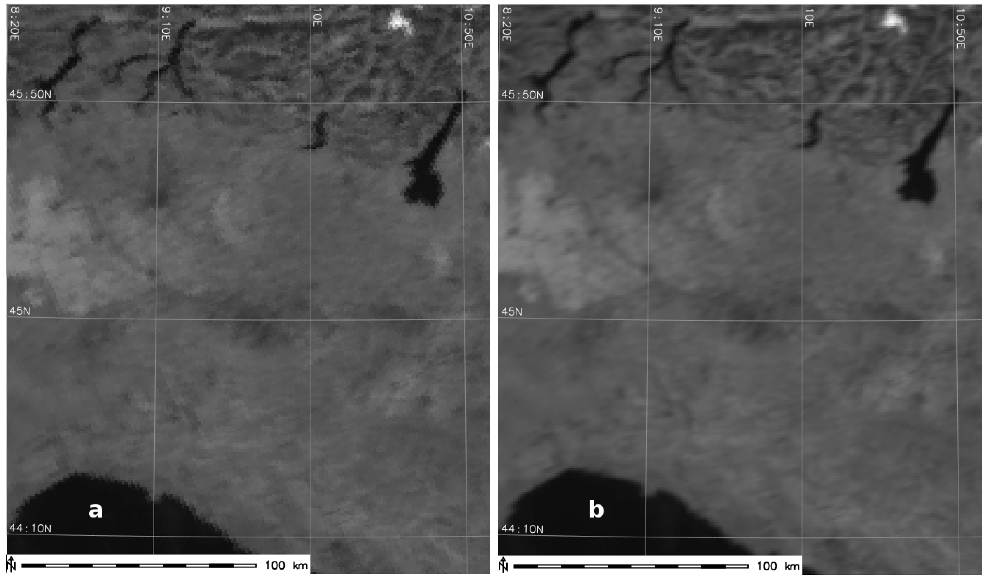
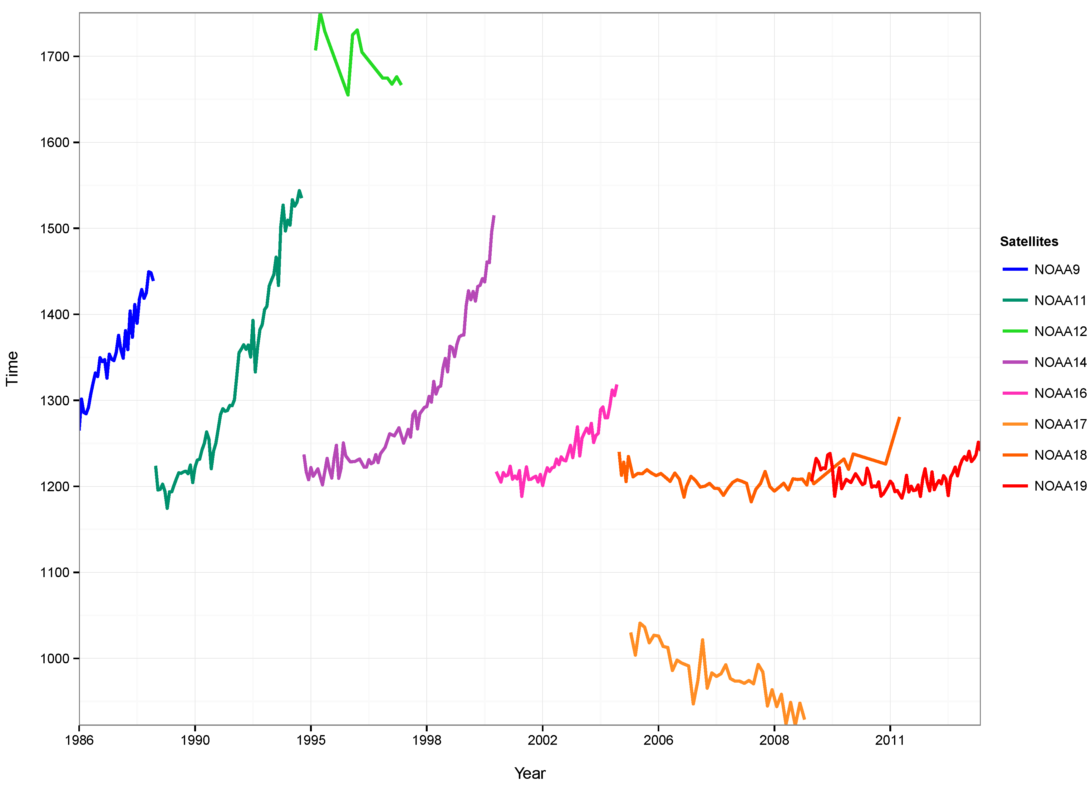
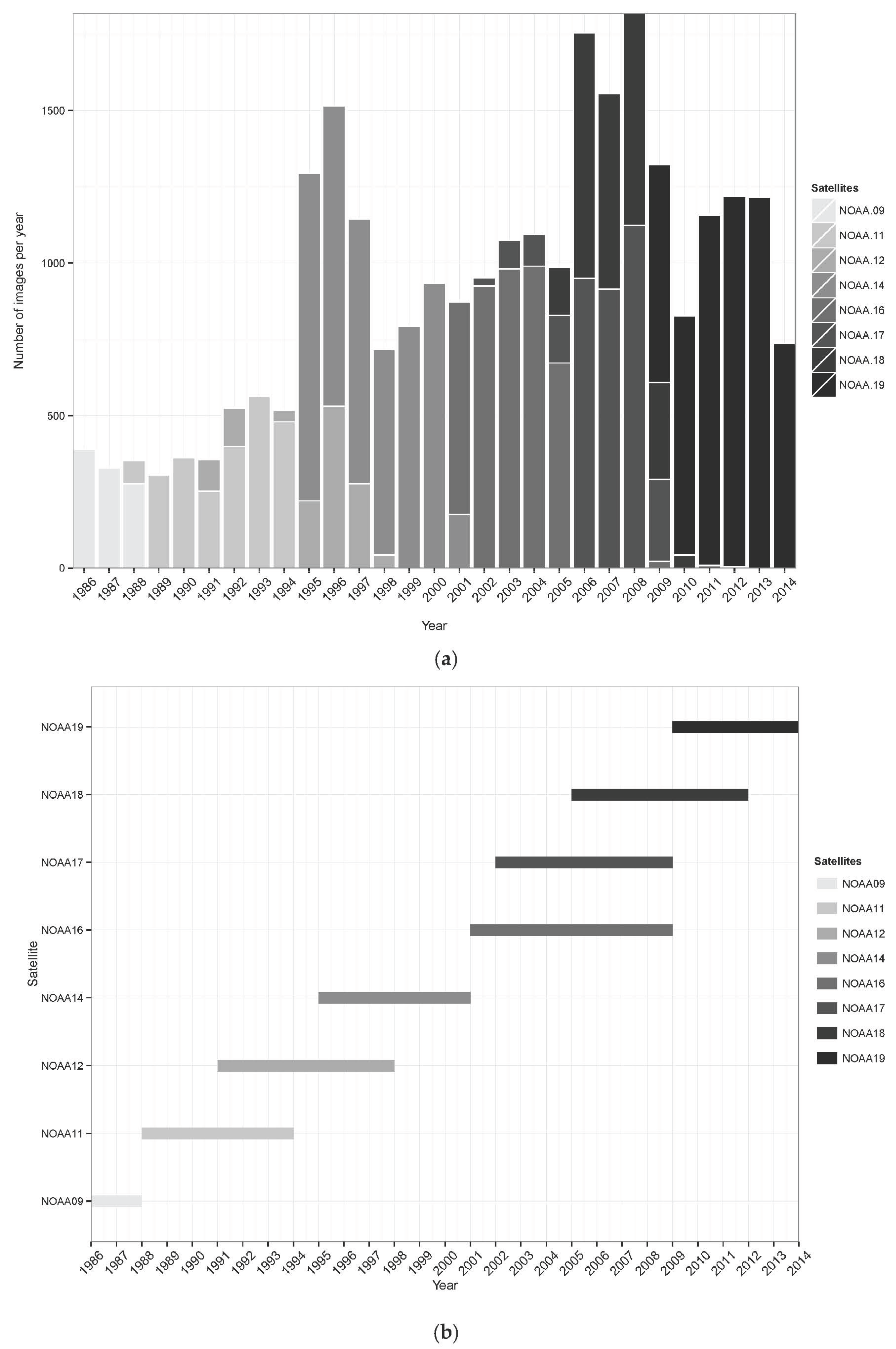
3.1. Time Series of Calibrated AVHRR LAC Data

The historical AVHRR LAC images at 1.1 km spatial resolution available for more than last 30 years is the longest time series of satellite data and a potential alternative to ground observations. Indeed, to develop the longest satellite derived time series of AVHRR LAC data, it is inevitable to combine data from multiple instruments which in turn require superior inter-sensor consistent calibration [32,34]. A total of 22,507 input images were acquired and processed using the new method (Figure 2a,b). The newly developed AVHRR LAC data readers in pygac and the new mpop plugin works with all the level 1B data across the POD and KLM series of instruments from the CLASS archive [6]. The code segment to read the POD and KLM data using the new plugin in mpop is given in Appendix A. The new mpop plugin has been made available in a public repository with GNU general public license [31].
The thermal calibration applied to the data as conceived by [34] is robust and takes care of the inter-calibration between different NOAA instruments. A conclusive validation of the quality of calibration between NOAA instruments is beyond the scope of this study. Instead we did inter-platform comparison of estimated LSWT which is explained in SubSection 3.3. AVHRR is a wide angle ±55.4° sensor using the whisk broom technique to acquire large swath in one acquisition. Nevertheless, it is important to resolve the artifacts in the wider angles due to the bow-tie effects. Visual comparison of multiple images before and after the resampling shows that the gradient-search method eliminates the bow-tie effects restoring the original geometry over the edges [35]. Figure 4 compares the Nearest Neighbour resampling technique with our approach. Gradient search approach (Figure 4b) provides a clear geometry of the lakes in Northern Italy, while the Nearest Neighbour (Figure 4a) interpolation distorts the image making it impossible to capture the geometry of small objects like lakes.

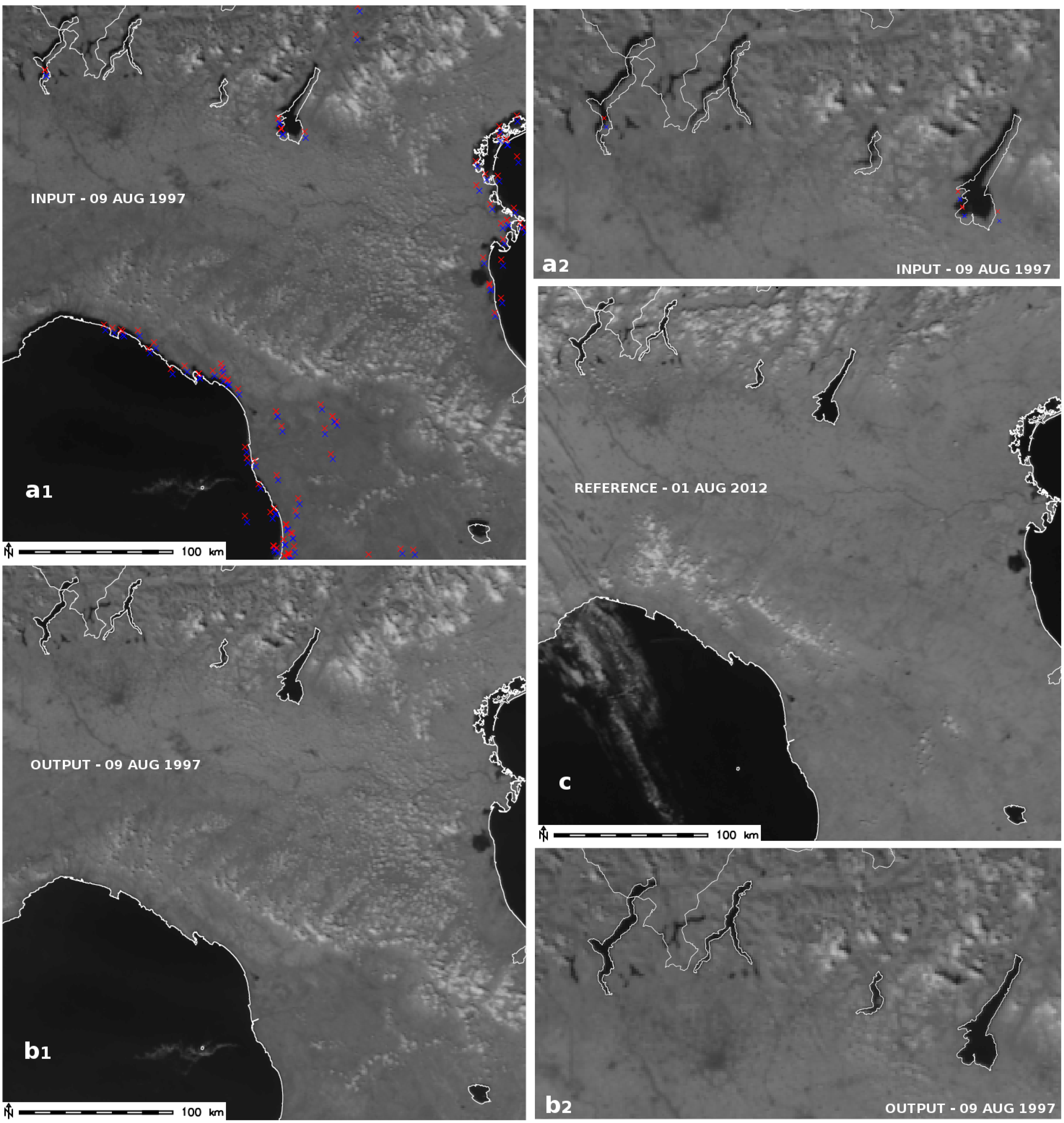
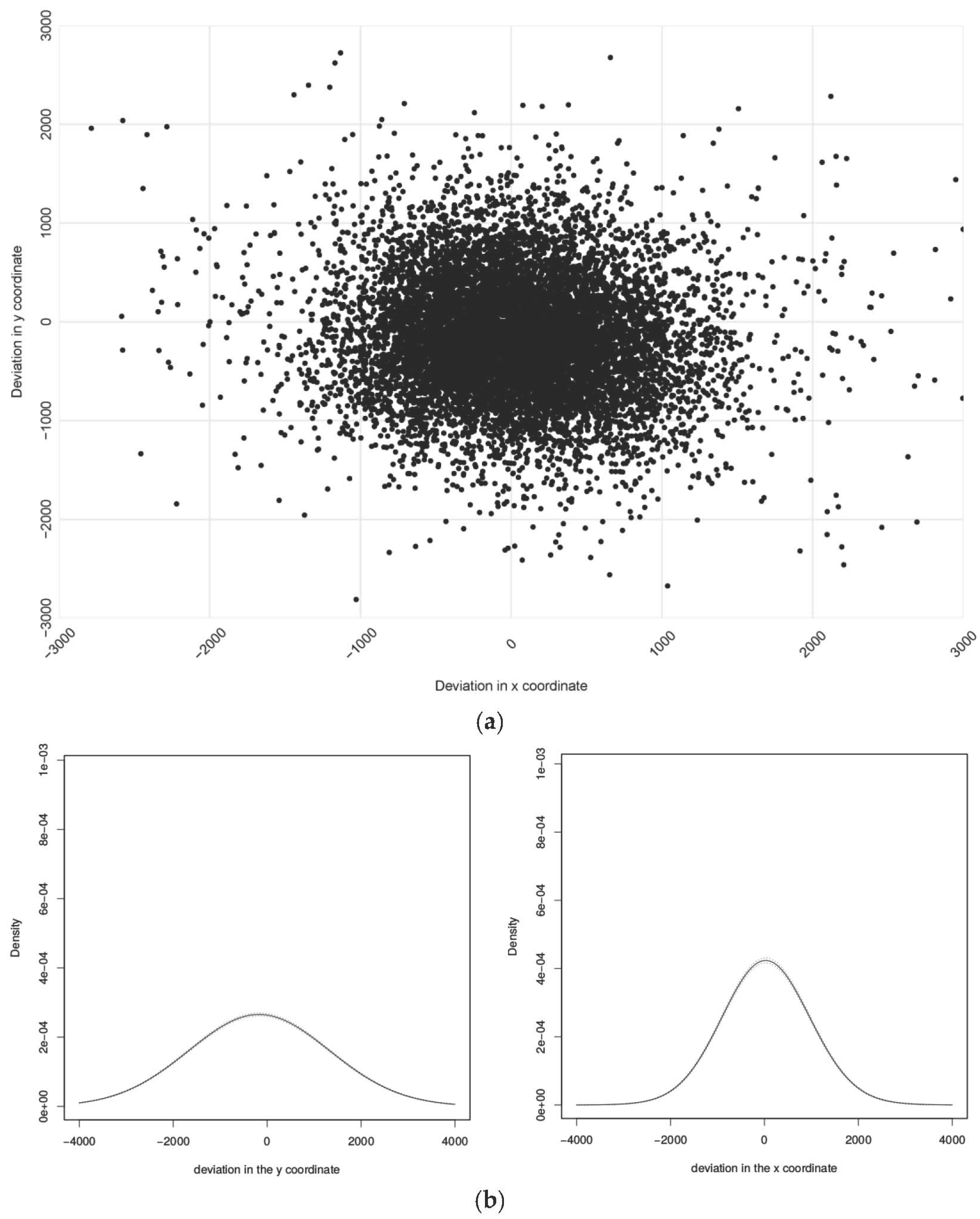
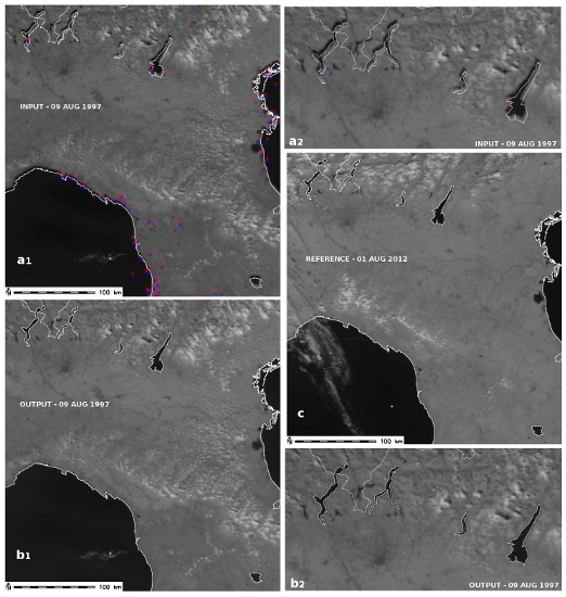
3.2. Geo-Rectification of Calibrated AVHRR LAC Data Using SIFT

We found that the number of extracted GCP’s using SIFT depends upon two major factors; (i) the overlapping area between the input and the reference image (ii) the cloud coverage. SIFT tends to fail on input images with cloud coverage more than 50% of the total area. On a clear sky image, combining all the corresponding bands, large number of GCP’s are extracted (> 300) for an area of 122,400 km2, which is then filtered iteratively to remove outliers (RMSE > 500 m). We observed that with large number of GCP’s, linear model rectification often failed due to islands of localized point clouds in the image. Hence we used the polynomial second order rectification for all the images irrespective of the number of GCP’s obtained from SIFT. Figure 5 shows different steps of the feature matching based geometric correction applied on a NOAA-14 AVHRR LAC image (POD) acquired on 9 August 1997. The input image is shown in Figure 5a (band 2-NIR) overlaid with the extracted GCP’s in which the position error is clearly visible along the national boundary and the lakes. Figure 5c shows the final output which is precisely aligned to the country and lake boundaries.
The validation output shows that the SIFT based geo-rectification procedure is able to achieve sub-pixel accuracy. Figure 6a shows the scatter plot of x deviation and y deviation of the GCP’s and Figure 6b shows the kernel density plots. The overall RMSE of 12,340 independent GCP’s from 2000 images is 755.63 m, which is below 1 pixel. The mean deviation in x and y direction is 607.82 m and 624.21 m respectively. The mean deviations are found to be on the same range suggesting that there is no geometric errors in either direction.

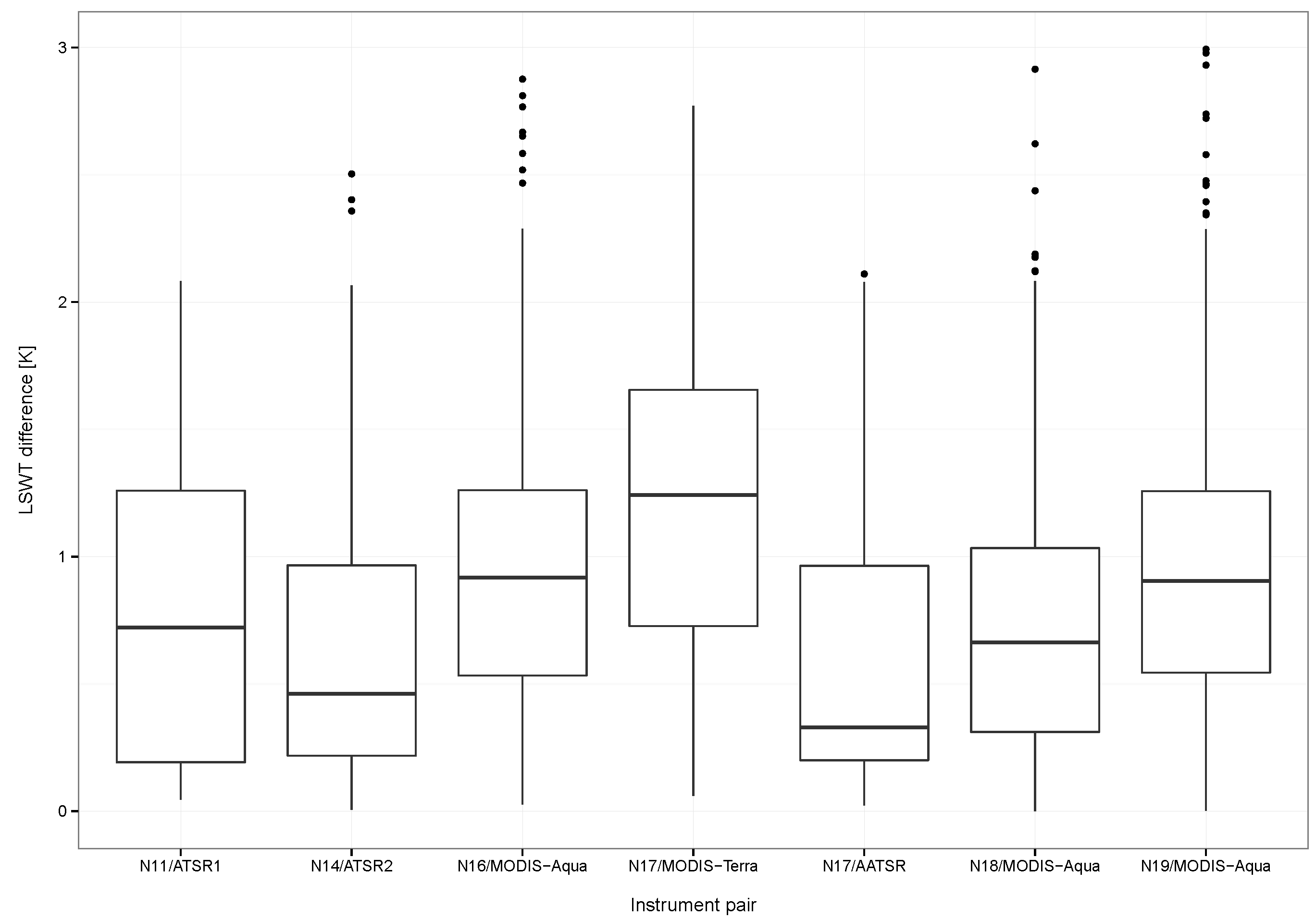
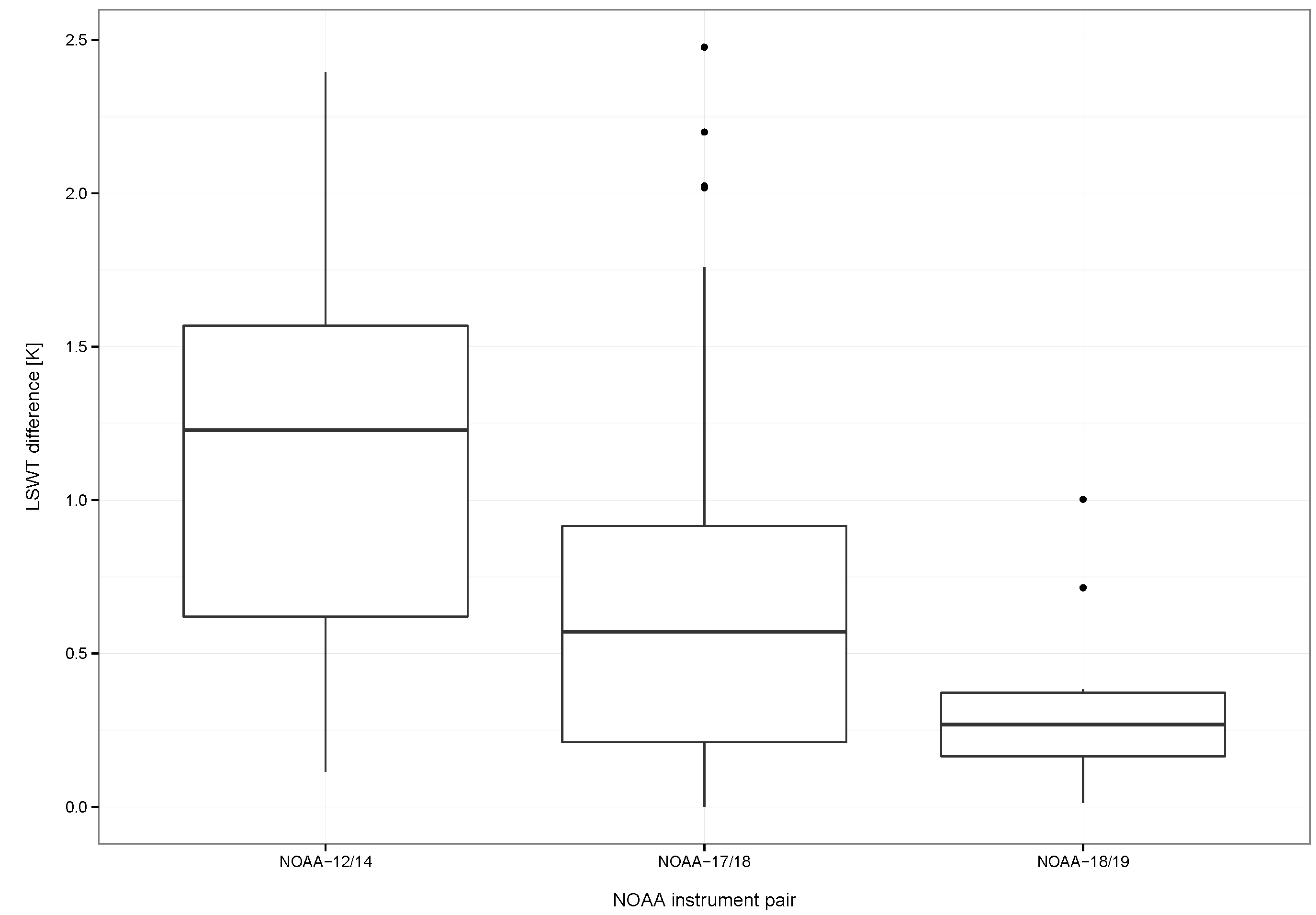
3.3. Quality Assessment of the Time Series Using Estimated LSWT

For the validation of the calibrated AVHRR LAC time series data, we compared the LSWT of the Lake Garda estimated from all the valid thermal channels, irrespective of the NOAA instrument, after pre-processing, geo-rectification and orbital drift correction [21]. Figure 7 shows boxplots of absolute lake mean LSWT differences between pair of NOAA instruments. The boxplots (Figure 7) are based on the same day observations by multiple NOAA instruments. We could only get three NOAA instrument pairs with same day observations for the inter-sensor comparison—NOAA-12/14, NOAA-17/18 and NOAA-18/19. The MAE for NOAA instrument pairs are 1.18 K, 0.67 K, 0.35 K for NOAA-12/14, NOAA-17/18 and NOAA-18/19 respectively. Moreover the RMSE is 1.36 K, 0.88 K and 0.44 K respectively.
Boxplots of the absolute lake mean LSWT differences between the cross-platform pairs are shown in Figure 8. The boxplots (Figure 8) are based on the same day observations by multiple instruments. The MAE and RMSE in all the cases are found to be between 0.5 K to 1.5 K (Table 3). In all the cases except for NOAA-17/MODIS-Terra, the median of lake mean LSWT difference lies below 1.5 K (Figure 8), which indicates that the majority of the differences are in the lower range of 0–1.5 K. The lowest MAE, RMSE of 0.6 K, 0.85 K respectively are reported with NOAA-17/AATSR observations, while the highest errors of 1.2 K, 1.35 K are with NOAA-17/MODIS-Terra (Table 3).
Table 4 lists important correlation statistics derived between LSWT and the in-situ data. Slopes are estimated from the linear models between LSWT from each NOAA instrument and the corresponding in-situ data. All the slope values are close to each other which shows the similar relationship between LSWT and in-situ data irrespective of the NOAA instrument. In all the cases, coefficient of determination R2 is higher than 0.93. An average RMSE and MAE of 0.92 K and 0.71 K are reported from the models.

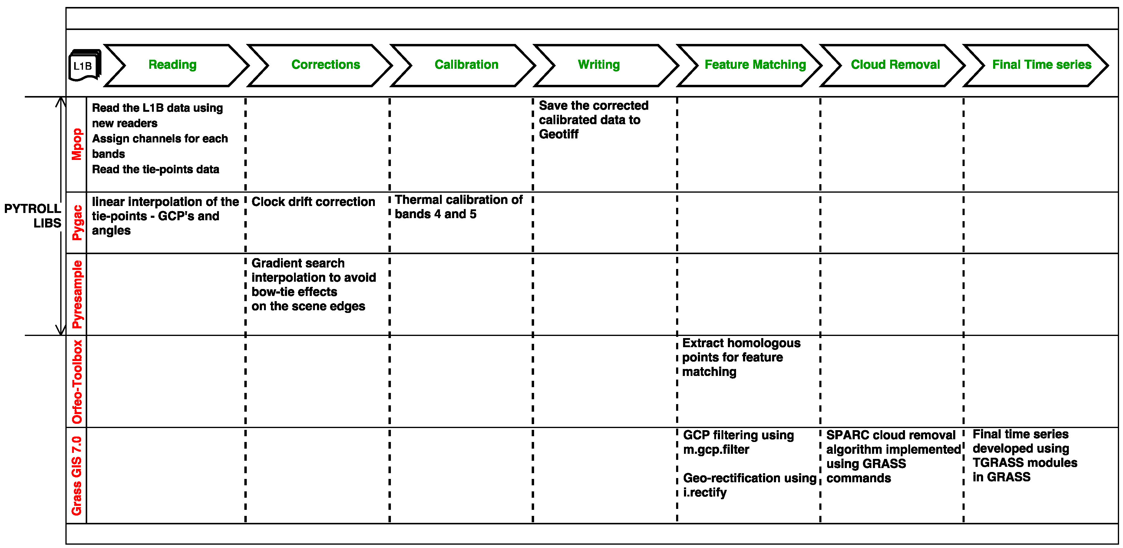
3.4. Software Code for Deploying the Method Elsewhere

To enable reproducibility of our method following [44] and [45] we publish the code snippets used to process the entire AVHRR LAC data. Appendix A is the Python script to process the AVHRR LAC data using the Pytroll libraries—mpop, pyresample, pygac—which will read level 1B format, apply solar and thermal calibration, resample using gradient search method, write all the channels and viewing zenith angle to image format. Appendix B is a bash script which is the second part of processing where the output images from Python script are processed inside GRASS GIS session. The bash script executes the SIFT matching using Orfeo toolbox, GCP filtering, geo-rectification and cloud removal.

4. Discussion

In this study we introduced a new automated method to accurately develop time series of AVHRR LAC data at 1 km spatial resolution covering 28 years from 1986–2014. The method is developed by chaining several open source geospatial packages (Table 2 and Figure 3) which is reproducible and extendable. To the best of our knowledge there are no other published studies which demonstrate successful processing of this data using tools which are available open to all researchers. The new additions to the Pytroll libraries—mpop and pygac—support all the AVHRR LAC data in level 1B format irrespective of the NOAA instrument, version of the AVHRR sensor and the various data header types released by NOAA [31]. Validation of automated geo-rectification of all the AVHRR LAC data using independent GCP’s extracted from 2000 randomly selected images reported sub-pixel accuracy with an overall RMSE of 755.63 m. The thermal calibration takes care of inter-platform variations [34] and our validation procedure shows that the same day LSWT estimated from AVHRR on-board different NOAA instruments are close to each other with overall mean absolute differences (Figure 7) below 1.5 K. Furthermore, the cross-platform validation also exhibited promising results with reported MAE and RMSE between 0.5 to 1.5 K (Figure 7).
One of the important aspects of this methodology is its ability to deal with the earlier AVHRR LAC data from POD satellites [3,12,14]. As proved by earlier studies [1,2,5], it is difficult to achieve accurate geo-rectification between temporal AVHRR images acquired from POD satellites. In order to achieve precise navigation, we applied feature matching technique—SIFT to extract homologous GCP’s [28,40]. We found that with this approach, high quality GCP’s can be extracted after applying an iterative filter based on RMSE. The independent GCP’s produced to validate the geo-rectification showed that the majority (>80%) of the GCP displacements either in x and y directions are in the sub-pixel range (Figure 6a). The reason for larger GCP displacements (>1000 m) could be that SIFT failed due to the cloud coverage or due to isolated cases of spurious calibration. To derive any meaningful long term bio-physical variables from the AVHRR LAC data it is crucial to take care of the inter-platform calibration which enables continuity of data over the transition of instruments [9,32,34]. Furthermore, the orbital drift (Figure 1) experienced with the earlier NOAA satellites poses a serious challenge to develop high quality time series data [21,46]. However, the acquisition time correction procedure based on the DTC model shows promising results towards homogenizing data from multiple satellites. The inter-platform validation of LSWT shows that the data are indeed comparable and that it is possible to combine the data over time to create longer time series (see Figure 7 and Table 3) [21]. The median of the inter-platform boxplots (Figure 7) are all below 1.5 K depicting the superior thermal calibration (Figure 7). Moreover, with the cross-platform validation we showed that the developed LSWT from AVHRR LAC data are close to those from similar sensors on-board instruments other than NOAA. We found exceptionally good agreement between NOAA-17 and AATSR, both morning overpasses, with lowest MAE and RMSE of 0.6 K and 0.85 K. On the other hand, the highest MAE and RMSE of 1.2 K and 1.35 K is reported between NOAA-17 and MODIS-Terra in spite of both being morning overpass data, which needs to be further investigated (Table 4). The outliers in both inter-platform and cross-platform boxplots could be due to undetected clouds, unresolved navigational errors or isolated cases of spurious thermal calibration. Though the validation with in-situ data show good agreement, it is important to note that the satellite sensor measures temperature of a sub-micron layer between water surface and air which is highly variable according to the meteorological conditions, whereas in-situ data represents bulk temperatures in the lake [47,48]. Due to the skin effect over the lake surface there is a considerable difference between the skin and bulk temperature which may also reflect the actual differences between satellite derived LSWT and the in-situ data [46,48]. The accuracy of the derived LSWT also depends upon the viewing zenith angle at which the observation is taken (nadir or wide angle) [43].
The developed method is fully automated which will enable the users to process bulk data in a single workflow. [44] emphasizes the need for adopting Stallman’s four freedom paradigms in ecological research. With the growing interest in open research and publishing the data publicly it is also important to have the software packages used in ecological research in a public domain [45]. Thus by taking advantage of the development of open source geospatial libraries over the last decade, we successfully revisited the accurate navigation of AVHRR LAC data and implemented a robust methodology to process them. Though the method is robust, manually checking the precision of each of the thousands of images is not practical, there could be unresolved navigational errors in the final time series. The automated cloud masking may also leave undetected cloud pixels as clear sky ones. Though the overall accuracy of SIFT based geo-rectification procedure is found to perform well within the extent of a pixel, it does not always ensure accurate positioning of inland pixels especially in mountainous terrain like the surroundings of Lake Garda. Our procedure does not correct for the surface elevation which may lead to pixel misplacements and could have adversary effects especially on small features like lakes. [19] explains accurate geolocation of AVHRR historical time series which includes a orthocorrection scheme taking care of the accurate positioning of the pixels in complicated terrains. Hence it is very important to design and perform robust statistical outlier detection before any trend analysis is performed with the developed time series data. Moreover, while we tested this method for a small study area covering Northern Italy, it can be extended to any other area provided the data are in level 1B format and obtained from the NOAA CLASS archive [6]. It is recommended to use high performance computing solutions if you are processing 28 years of AVHRR data over a larger area. An ideal way to compare the performance of different sensors is the simultaneous nadir observations approach, but it is unlikely to obtain such a pair of images over our study area [49].
The flagship NOAA series of instruments ended with NOAA-19, though the AVHRR radiometer continued aboard the MetOp-A and MetOp-B satellites as part of a collaborative meteorological program by the European Space Agency and the European organization for the exploitation of meteorological satellites. However, data from MetOp series are not considered in this study to focus exclusively on NOAA instruments. The methodology also works with solar channels of AVHRR [32], though it is not the scope of this paper to validate the performance of solar calibration. For the SIFT method, bringing a seasonal perspective by using different reference images for multiple seasons (or months) may improve the quality of the extracted GCP’s [19]. It has to be noted that for inter-platform and cross-platform validation, we took the same day observations between 08:00 to 17:00 UTC which is a wide window and explains some of the outliers in spite of performing the acquisition time correction procedure. The gaps in the final time series after cloud masking and the outlier removal could be statistically filled using methods like harmonic analysis [50] and spatio-temporal modelling [51]. We avoided night time acquisitions as the specific project objectives demanded processing of day time data and due to non-availability of field data during night time to validate the product. In general, checking the consistency with night time data is important to make complete use of the AVHRR dual acquisitions. It is recommended to use a long term high frequent in-situ data for validating the satellite derived products to match the time of observations. Comparing the long-term trends from both in-situ data and satellite derived LSWT would be a recommended approach in testing the temporal stability of AVHRR LAC data over transition of instruments [46]. But due to lack of high frequent in-situ data we avoided comparing the long term trends, instead we used linear models to check the integrity of derived LSWT. For LSWT estimation, we used a generic non-linear split window equation (Equation (1)), but using satellite specific coefficients provided by [42]. However, previous studies [21,43] have shown that lake specific coefficients will lead to accurate LSWT estimation. Due to non-availability of lake specific coefficients for the POD satellites [43] and other non AVHRR sensors [21], it is difficult to follow the same method to derive LSWT from all the satellites used in this study. Nevertheless, we obtained high accuracy (see Table 3 and Table 4) by using satellite specific coefficients in a non-linear split window equation.

5. Conclusions

To conclude, in this paper we present a new automated method for processing historical AVHRR LAC data using open source geospatial packages (Figure 3). The method is extendable and reproducible to any other geographic location provided the data is taken from NOAA CLASS archive. All the software development related to this work is been published in public archives making it accessible to maximum potential users [30] (Table 2). We found that it is possible to resolve the much documented navigational errors with the AVHRR LAC data from POD satellites by implementing a robust geo-rectification procedure using SIFT feature extraction procedure. This automated geo-rectification procedure produced promising results and the validation using independent GCP’s reported an overall RMSE of 755.63 m. Further we did a three step validation procedure for the derived time series of brightness temperatures, (i) inter-platform validation by comparing estimated LSWT’s between different NOAA instruments; (ii) cross-platform validation by comparing estimated LSWT’s between NOAA instruments and other polar orbiting sensors like MODIS and AATSR; (iii) validation using in-situ data (Table 3 and Table 4). The overall RMSE reported for inter-platform, cross-platform and in-situ validation are 0.89 K, 1.05 K and 0.92 K respectively. The high accuracy obtained with the validation procedure after performing an acquisition time correction procedure based on DTC model shows that it is indeed possible to develop a homogenized dataset from AVHRR LAC data over multiple NOAA instruments. Our new method, along with the code snippets (Appendices A and B) to process AVHRR LAC data will enable researchers to leverage the availability of historical medium resolution AVHRR data in their research, otherwise impossible to use due to well documented issues [1,2,4]. It takes care of multiple sources of errors to a large extent giving an opportunity to develop a homogenized time series of brightness temperatures from AVHRR LAC data. The new methodology opens a new paradigm for researchers to create long term (28 years) daily temporal datasets of land/water surface temperature derived from satellite imageries. It should be noted that the current study is validated only for lake surface temperature. For land surface, corresponding changes must be made on the split window algorithm and the coefficients. The effects of orbital drift will also vary depending on the land use demanding case specific correction procedures. It is recommended to establish robust statistical filtering methods to remove undetected outliers before performing any trend analysis using the derived data. The data thus derived can play a significant role in research as an alternative to long term field measurements. Moreover, we could not find any public dataset derived from AVHRR data available at its original spatial resolution. Much of the earlier AVHRR data are underused due to lack of software tools to accurately process them. This study will fill this gap and give scientists the opportunity to use the AVHRR LAC data at its original spatial resolution for their research.

Acknowledgments

The PhD Scholarship of Sajid Pareeth is supported by FIRS>T (FEM International Research School e Trentino) of Fondazione Edmund Mach, Italy. We acknowledge NOAA for providing historical AVHRR LAC data in level 1B format through the CLASS archive. We also acknowledge EUMETSAT for providing European reanalysis data. We acknowledge NASA and ESA for providing MODIS and ATSR series data in public through LAADS and MERCI respectively. We sincerely thank Juan-Carlos Jimenez-Muñoz of University of Valencia, for publishing the satellite specific split-window coefficients and providing us with the missing ones upon request. We acknowledge the communities behind the development and fine-tuning of the open source geospatial packages, especially the ones used here—Pytroll, Orfeo toolbox and GRASS GIS for their valuable support through mailing lists and personal communications. We also thank the anonymous reviewers for their critical reading and suggestions which substantially helped to improve the manuscript.

Author Contributions

The idea was conceived by Sajid Pareeth, Markus Neteler and Nico Salmaso. The software development was done primarily by Sajid Pareeth with the support of Luca Delucchi, Markus Neteler, Markus Metz, Abhay Devasthale and Martin Raspaud. Sajid Pareeth, Markus Neteler and Duccio Rocchini contributed to the statistical analyses. All authors contributed to the writing.

Conflicts of Interest

The authors declare no conflict of interest.

Abbreviations

AATSR: Advanced Along-Track Scanning Radiometer
ATSR: Along Track Scanning Radiometer
AVHRR: Advanced Very High Resolution Radiometer
CLASS: Comprehensive Large Array-data Stewardship System
DTC: Diurnal Temperature Cycle
ECMWF: European Center for Medium-range Weather Forecasts
GCP: Ground Control Point
GIS: Geographic Information System
GPL: General Public License
GRASS: Geographic Resources Analysis Support System
K: Kelvin
LAC: Local Area Coverage
LSWT: Lake Surface Water Temperature
MAE: Mean Absolute Error
MetOp: Meteorological Operational
MODIS: Moderate Resolution Imaging Spectroradiometer
NIR: Near Infrared
NOAA: National Oceanic and Atmospheric Administration
POD: Polar Orbiter Data
RMSE: Root Mean Square Error
SIFT: Scale Invariant Feature Transform
SPARC: Separation of Pixels Using Aggregated Rating over Canada
TIROS: Television Infrared Observation Satellite
UTC: Coordinated Universal Time

Appendix

A. Python Script to Read and Calibrate Level 1B AVHRR LAC Data Using Pytroll Libraries

Remotesensing 08 00169 i001
Remotesensing 08 00169 i002
Remotesensing 08 00169 i003

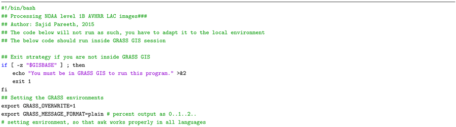
B. Bash Script to Process the Level 1B AVHRR LAC Data—Entire Workflow

Note about script formatting: Long lines are broken with \\which means that the command continues on the next line. This symbol is usually not necessary when typing but it is used here for formatting reasons.
Remotesensing 08 00169 i004
Remotesensing 08 00169 i005
Remotesensing 08 00169 i006
Remotesensing 08 00169 i007
Remotesensing 08 00169 i008
Remotesensing 08 00169 i009

References

  1. Brunel, P.; Marsouin, A. Operational AVHRR navigation results. Int. J. Remote Sens. 2000, 21, 951–972. [Google Scholar] [CrossRef]
  2. Privette, J.; Fowler, C.; Wick, G.; Baldwin, D.; Emery, W. Effects of orbital drift on advanced very high resolution radiometer products: Normalized difference vegetation index and sea surface temperature. Remote Sens. Environ. 1995, 53, 164–171. [Google Scholar] [CrossRef]
  3. Baldwin, D.; Emery, W.J. Spacecraft attitude variations of NOAA-11 inferred from AVHRR imagery. Int. J. Remote Sens. 1995, 16, 531–548. [Google Scholar] [CrossRef]
  4. Krasnopolsky, V.M.; Breaker, L.C. The problem of AVHRR image navigation revisited. Int. J. Remote Sens. 1994, 15, 979–1008. [Google Scholar] [CrossRef]
  5. Emery, W.J.; Brown, J.; Nowak, Z.P. AVHRR image navigation - Summary and review. Photogramm. Eng. Remote Sens. 1989, 4, 1175–1183. [Google Scholar]
  6. Comprehensive Large Array-Data Stewardship System NOAA Data. Available online: http://www.class.ncdc.noaa.gov/ ( accessed on 29 July 2015).
  7. Cracknell, A.P. Advanced Very High Resolution Radiometer AVHRR, 1st ed.; CRC Press: Bristol, PA, USA, 1997. [Google Scholar]
  8. NOAA KLM LAC Data Set Header Records. Available online: http://www.ncdc.noaa.gov/oa/pod-guide/ncdc/docs/klm/html/c8/sec83132-2.htm#t8313221 (accessed on 14 June 2015).
  9. Trishchenko, A.P.; Fedosejevs, G.; Li, Z.; Cihlar, J. Trends and uncertainties in thermal calibration of AVHRR radiometers onboard NOAA-9 to NOAA-16. J. Geophys. Res. Atmos. 2002, 107, 4778. [Google Scholar] [CrossRef]
  10. NOAA POD LAC Data Set Header Records. Available online: http://www.ncdc.noaa.gov/oa/pod-guide/ncdc/docs/podug/html/c2/sec2-0.htm (accessed on 14 June 2015).
  11. Price, J.C. Timing of NOAA afternoon passes. Int. J. Remote Sens. 1991, 12, 193–198. [Google Scholar] [CrossRef]
  12. Kaufmann, R.; Zhou, L.; Knyazikhin, Y.; Shabanov, V.; Myneni, R.; Tucker, C. Effect of orbital drift and sensor changes on the time series of AVHRR vegetation index data. IEEE Trans. Geosci. Remote Sens. 2000, 38, 2584–2597. [Google Scholar]
  13. Historical TLE Records. Available online: http://celestrak.com/ (accessed on 14 June 2015).
  14. Rosborough, G.; Baldwin, D.; Emery, W. Precise AVHRR image navigation. IEEE Trans. Geosci. Remote Sens. 1994, 32, 644–657. [Google Scholar] [CrossRef]
  15. Bordes, P.; Brunel, P.; Marsouin, A. Automatic Adjustment of AVHRR Navigation. J. Atmos. Ocean. Technol. 1992, 9, 15–27. [Google Scholar] [CrossRef]
  16. Fontana, F.M.; Coops, N.C.; Khlopenkov, K.V.; Trishchenko, A.P.; Riffler, M.; Wulder, M.A. Generation of a novel 1km NDVI data set over Canada, the northern United States, and Greenland based on historical AVHRR data. Remote Sens. Environ. 2012, 121, 171–185. [Google Scholar] [CrossRef]
  17. Moreno, J.; Melia, J. A method for accurate geometric correction of NOAA AVHRR HRPT data. IEEE Trans. Geosci. Remote Sens. 1993, 31, 204–226. [Google Scholar] [CrossRef]
  18. Latifovic, R.; Trishchenko, A.P.; Chen, J.; Park, W.B.; Khlopenkov, K.V.; Fernandes, R.; Pouliot, D.; Ungureanu, C.; Luo, Y.; Wang, S.; et al. Generating historical AVHRR 1 km baseline satellite data records over Canada suitable for climate change studies. Can. J. Remote Sens. 2005, 31, 324–346. [Google Scholar] [CrossRef]
  19. Khlopenkov, K.; Trishchenko, A.; Luo, Y. Achieving Subpixel Georeferencing Accuracy in the Canadian AVHRR Processing System. IEEE Trans. Geosci. Remote Sens. 2010, 48, 2150–2161. [Google Scholar] [CrossRef]
  20. Hüsler, F.; Fontana, F.; Neuhaus, C.; Riffler, M.; Musial, J.; Wunderle, S. AVHRR archive and processing Facility at the university of Bern: A comprehensive 1-km satellite data set for climate change studies. EARSeL eProc. 2011, 10, 83–101. [Google Scholar]
  21. Riffler, M.; Lieberherr, G.; Wunderle, S. Lake surface water temperatures of European Alpine lakes (1989–2013) based on the Advanced Very High Resolution Radiometer (AVHRR) 1 km data set. Earth Syst. Sci. Data 2015, 7, 1–17. [Google Scholar] [CrossRef]
  22. Brovelli, M.A.; Mitasova, H.; Neteler, M.; Raghavan, V. Free and open source desktop and Web GIS solutions. Appl. Geomat. 2012, 4, 65–66. [Google Scholar] [CrossRef]
  23. Neteler, M.; Bowman, M.H.; Landa, M.; Metz, M. GRASS GIS: A multi-purpose open source GIS. Environ. Model. Softw. 2012, 31, 124–130. [Google Scholar] [CrossRef]
  24. Pytroll Home Page. Available online: http://www.pytroll.org/ (accessed on 14 June 2015).
  25. Inglada, J.; Christophe, E. The Orfeo Toolbox Remote Sensing Image Processing Software. In Proceedings of the 2009 IEEE International Geoscience and Remote Sensing Symposium (IGARSS), Cape Town, South Africa, 12–17 July 2009; pp. 733–736.
  26. GRASS Development Team. Geographic Resources Analysis Support System (GRASS GIS) Software; Open Source Geospatial Foundation: USA, 2015. Available online: http://grass.osgeo.org (accessed on 16 February 2016).
  27. Neteler, M.; Mitasova, H. Open Source GIS: A GRASS GIS Approach; Springer: New York, NY, USA, 2008. [Google Scholar]
  28. Lowe, D.G. Distinctive image features from scale-invariant keypoints. Int. J. Comput. Vis. 2004, 60, 91–110. [Google Scholar] [CrossRef]
  29. m.gcp.filter man. Available online: https://grass.osgeo.org/grass70/manuals/addons/m.gcp.filter.html (accessed on 20 October 2015).
  30. Pygac Git Repository. Available online: https://github.com/adybbroe/pygac (accessed on 14 June 2015).
  31. Mpop Git Repository. Available online: https://github.com/pytroll/mpop (accessed on 14 June 2015).
  32. Heidinger, A.K.; Straka, W.C.; Molling, C.C.; Sullivan, J.T.; Wu, X. Deriving an inter-sensor consistent calibration for the AVHRR solar reflectance data record. Int. J. Remote Sens. 2010, 31, 6493–6517. [Google Scholar] [CrossRef]
  33. Cao, C.; Weinreb, M.; Sullivan, J. Solar contamination effects on the infrared channels of the advanced very high resolution radiometer (AVHRR). J. Geophys. Res. 2001, 106, 33463. [Google Scholar] [CrossRef]
  34. Trishchenko, A.P. Removing unwanted fluctuations in the AVHRR thermal calibration data using robust techniques. J. Atmos. Ocean. Technol. 2002, 19, 1939–1954. [Google Scholar] [CrossRef]
  35. Khlopenkov, K.; Trishchenko, A. Implementation and evaluation of concurrent gradient search method for reprojection of MODIS level 1B imagery. IEEE Trans. Geosci. Remote Sens. 2008, 46, 2016–2027. [Google Scholar] [CrossRef]
  36. Khlopenkov, K.V.; Trishchenko, A.P. SPARC: New cloud, snow, and cloud shadow detection scheme for historical 1-km AVHHR data over Canada. J. Atmos. Ocean. Technol. 2007, 24, 322–343. [Google Scholar] [CrossRef]
  37. Dee, D.P.; Uppala, S.M.; Simmons, A.J.; Berrisford, P.; Poli, P.; Kobayashi, S.; Andrae, U.; Balmaseda, M.A.; Balsamo, G.; Bauer, P.; et al. The ERA-Interim reanalysis: Configuration and performance of the data assimilation system. Q. J. R. Meteorol. Soc. 2011, 137, 553–597. [Google Scholar] [CrossRef]
  38. Lowe, D. Object recognition from local scale-invariant features. In Proceedings of the Seventh IEEE International Conference on Computer Vision, Kerkyra, Greece, 20–27 September 1999; pp. 1150–1157.
  39. Yu, L.; Zhang, D.; Holden, E.J. A fast and fully automatic registration approach based on point features for multi-source remote-sensing images. Comput. Geosci. 2008, 34, 838–848. [Google Scholar] [CrossRef]
  40. Fan, B.; Huo, C.; Pan, C.; Kong, Q. Registration of Optical and SAR Satellite Images by Exploring the Spatial Relationship of the Improved SIFT. IEEE Geosci. Remote Sens. Lett. 2013, 10, 657–661. [Google Scholar] [CrossRef]
  41. Rocchini, D.; Di Rita, A. Relief effects on aerial photos geometric correction. Appl. Geogr. 2005, 25, 159–168. [Google Scholar] [CrossRef]
  42. Jimenez-Munoz, J.C.; Sobrino, J. Split-Window Coefficients for Land Surface Temperature Retrieval From Low-Resolution Thermal Infrared Sensors. IEEE Geosci. Remote Sens. Lett. 2008, 5, 806–809. [Google Scholar] [CrossRef]
  43. Hulley, G.C.; Hook, S.J.; Schneider, P. Optimized split-window coefficients for deriving surface temperatures from inland water bodies. Remote Sens. Environ. 2011, 115, 3758–3769. [Google Scholar] [CrossRef]
  44. Rocchini, D.; Neteler, M. Let the four freedoms paradigm apply to ecology. Trends Ecol. Evolut. 2012, 27, 310–311. [Google Scholar] [CrossRef] [PubMed]
  45. Reichman, O.J.; Jones, M.B.; Schildhauer, M.P. Challenges and Opportunities of Open Data in Ecology. Science 2011, 331, 703–705. [Google Scholar] [CrossRef] [PubMed]
  46. Schneider, P.; Hook, S.J. Space observations of inland water bodies show rapid surface warming since 1985. Geophys. Res. Lett. 2010, 37, L22405. [Google Scholar] [CrossRef]
  47. Wilson, R.C.; Hook, S.J.; Schneider, P.; Schladow, S.G. Skin and bulk temperature difference at Lake Tahoe: A case study on lake skin effect. J. Geophys. Res. Atmos. 2013, 118, 10332–10346. [Google Scholar] [CrossRef]
  48. Hook, S.J.; Prata, F.J.; Alley, R.E.; Abtahi, A.; Richards, R.C.; Schladow, S.G.; Pálmarsson, S. Retrieval of Lake Bulk and Skin Temperatures Using Along-Track Scanning Radiometer (ATSR-2) Data: A Case Study Using Lake Tahoe, California. J. Atmos. Ocean. Technol. 2003, 20, 534–548. [Google Scholar] [CrossRef]
  49. Karlsson, K.G.; Johansson, E. Multi-Sensor Calibration Studies of AVHRR-Heritage Channel Radiances Using the Simultaneous Nadir Observation Approach. Remote Sens. 2014, 6, 1845–1862. [Google Scholar] [CrossRef]
  50. Roerink, G.J.; Menenti, M.; Verhoef, W. Reconstructing cloudfree NDVI composites using Fourier analysis of time series. Int. J. Remote Sens. 2000, 21, 1911–1917. [Google Scholar] [CrossRef]
  51. Metz, M.; Rocchini, D.; Neteler, M. Surface temperatures at the continental scale: Tracking changes with remote sensing at unprecedented detail. Remote Sens. 2014, 6, 3822–3840. [Google Scholar] [CrossRef]
Figure 1. Plot of variation in observation times of National Oceanic and Atmospheric Administration (NOAA) instruments, note the large orbital drifts of the earlier NOAA-9/11/12/14 instruments.
Remotesensing 08 00169 g001
Figure 2. Data distribution. (a) Distribution of AVHRR Local Area Coverage (LAC) images over study area from 1986 to 2014 obtained from NOAA Comprehensive Large Array-data Stewardship System (CLASS) archive, separated by different instruments; (b) Time line of NOAA instruments used in this study.
Remotesensing 08 00169 g002
Figure 3. Workflow diagram. On top, the horizontal arrows show the main steps involved in the workflow, the software are listed vertically on the left. Role of each software in the workflow is explained in the corresponding cells.
Remotesensing 08 00169 g003
Figure 4. NIR (Near Infrared) channel 2 of AVHRR LAC data resampled using (a) Nearest Neighbour interpolation; (b) interpolated using the gradient search algorithm. The image is NOAA-18 AVHRR LAC taken on 1 August 2011.
Remotesensing 08 00169 g004
Figure 5. (ac) explains geometric correction done on NOAA-14 AVHRR LAC data (NIR channel 2 shown here) acquired on 09 August 1997. (a1) The input image with lake and country boundaries overlayed. Also shown is blue (input) and red (reference) crosses, the Ground Control Points (GCPs) extracted using the SIFT algorithm; (b1) The reference image used to extract the GCP points, NOAA-19 AVHRR LAC acquired on 01 August 2012; (c) The NOAA-14 AVHRR LAC image after polynomial second level rectification using the GCP’s; (a2) Figure a1 zoomed to the sub-alpine lakes in Northern Italy; & (b2) Figure b1 zoomed to the sub-alpine lakes in Northern Italy.
Remotesensing 08 00169 g005
Figure 6. Validation of Scale Invariant Feature Transform (SIFT) algorithm. (a) Independent GCP point-cloud plotted in x-deviation, y-deviation; (b) Kernel density plot of x and y deviations.
Remotesensing 08 00169 g006
Figure 7. Boxplots of absolute difference between lake mean Lake Surface Water Temperature (LSWT) estimated from multiple NOAA same day observations; horizontal thick line inside the box represents median; lower and upper end of the box represents first and third quartiles respectively; the bottom whisker ranges from first quartile to the smallest non-outlier and the top whisker ranges from third quartile to the largest non-outlier; the dots outside whiskers are outliers.
Remotesensing 08 00169 g007
Figure 8. Boxplots of absolute difference between lake mean LSWT estimated from same day observations from NOAA and other instruments; horizontal thick line inside the box represents median; lower and upper end of the box represents first and third quartiles respectively; the bottom whisker ranges from first quartile to the smallest non-outlier and the top whisker ranges from third quartile to the largest non-outlier; the dots outside whiskers are outliers.
Remotesensing 08 00169 g008
Table 1. Spectral resolution of Advanced Very High Resolution Radiometer (AVHRR) sensors in μm.
ChannelsAVHRR/1AVHRR/2AVHRR/3
10.58–0.680.58–0.680.58–0.68
20.725–1.100.725–1.100.725–1.10
3aN.AN.A1.58–1.68
3b3.55–3.933.55–3.933.55–3.93
410.50–11.5010.3–11.310.3–11.3
5Ch.4 repeated11.5–12.511.5–12.5
Table 2. List of software packages used in this study (License type urls: http://www.gnu.org/copyleft/gpl.html, http://www.cecill.info/licences/Licence_CeCILL_V2-en.html).
SoftwareSourceVersionLicense
Pytroll/mpophttps://github.com/pytroll/mpop-GNU GPL v3
Pytroll/pygachttps://github.com/adybbroe/pygac-GNU GPL v3
Pytroll/pyresamplehttps://github.com/pytroll/pyresample/-GNU GPL v3
Orfeo Toolboxhttps://www.orfeo-toolbox.org/4.4.0CeCILL v2
GRASS GIShttp://grass.osgeo.org/7.0.0GNU GPL v3
Table 3. Mean Absolute Error (MAE) and Root Mean Square Error (RMSE) (in Kelvin) between lake mean LSWT estimated between pair of sensors.
Sensor pairN12/N14N17/N18N18/N19N11/ATS1N14/ATS2N17/AATSRN17/MODTN16/MODAN18/MODAN19/MODA
MAE1.180.670.350.810.720.61.20.990.750.95
RMSE1.360.880.441.00.980.851.351.160.921.12
N26751038982875149262385
N = Number of observations; N11 = NOAA-11 (likewise for other NOAA instruments - N11,N14,N16,N17,N18,N19); ATS = ATSR; MODT = MODIS-Terra; MODA = MODIS-Aqua.
Table 4. Correlation statistics between in-situ data and corresponding LSWT derived from various NOAA instruments; N = Number of samples used in the linear model.
SatellitesSlopeR2RMSEMAEN
NOAA-110.970.980.810.6512
NOAA-140.900.931.381.0522
NOAA-160.980.990.360.2810
NOAA-170.890.990.560.467
NOAA-180.980.971.040.7712
NOAA-190.920.941.401.0821

