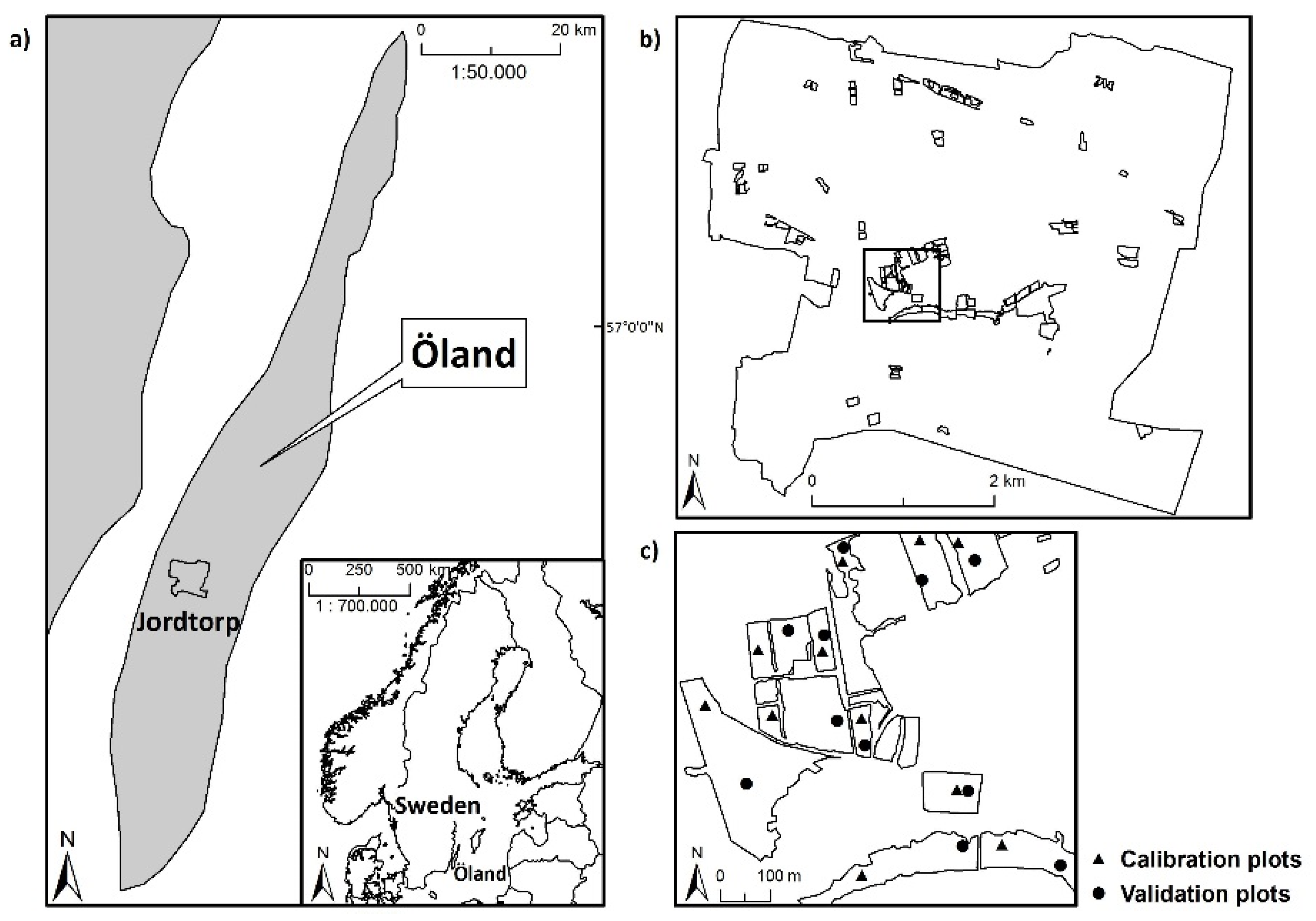
Article

Airborne Hyperspectral Data Predict Fine-Scale Plant Species Diversity in Grazed Dry Grasslands

1
Department of Grassland Science and Renewable Plant Resources, University of Kassel, Steinstrasse 19, 37213 Witzenhausen, Germany
2
Department of Physical Geography and Ecosystem Sciences, Lund University, Sölvegatan 12, 223 62 Lund, Sweden
3
Department of Biology, Lund University, Sölvegatan 37, 223 62 Lund, Sweden
*
Author to whom correspondence should be addressed.
Remote Sens. 2016, 8(2), 133; https://doi.org/10.3390/rs8020133
Submission received: 16 September 2015 / Revised: 3 December 2015 / Accepted: 25 January 2016 / Published: 8 February 2016
(This article belongs to the Special Issue Remote Sensing of Biodiversity)

Abstract

:
Semi-natural grasslands with grazing management are characterized by high fine-scale species richness and have a high conservation value. The fact that fine-scale surveys of grassland plant communities are time-consuming may limit the spatial extent of ground-based diversity surveys. Remote sensing tools have the potential to support field-based sampling and, if remote sensing data are able to identify grassland sites that are likely to support relatively higher or lower levels of species diversity, then field sampling efforts could be directed towards sites that are of potential conservation interest. In the present study, we examined whether aerial hyperspectral (414–2501 nm) remote sensing can be used to predict fine-scale plant species diversity (characterized as species richness and Simpson’s diversity) in dry grazed grasslands. Vascular plant species were recorded within 104 (4 m × 4 m) plots on the island of Öland (Sweden) and each plot was characterized by a 245-waveband hyperspectral data set. We used two different modeling approaches to evaluate the ability of the airborne spectral measurements to predict within-plot species diversity: (1) a spectral response approach, based on reflectance information from (i) all wavebands, and (ii) a subset of wavebands, analyzed with a partial least squares regression model, and (2) a spectral heterogeneity approach, based on the mean distance to the spectral centroid in an ordinary least squares regression model. Species diversity was successfully predicted by the spectral response approach (with an error of ca. 20%) but not by the spectral heterogeneity approach. When using the spectral response approach, iterative selection of important wavebands for the prediction of the diversity measures simplified the model but did not improve its predictive quality (prediction error). Wavebands sensitive to plant pigment content (400–700 nm) and to vegetation structural properties, such as above-ground biomass (700–1300 nm), were identified as being the most important predictors of plant species diversity. We conclude that hyperspectral remote sensing technology is able to identify fine-scale variation in grassland diversity and has a potential use as a tool in surveys of grassland plant diversity.

Graphical Abstract

1. Introduction

The threats to biodiversity from habitat loss, fragmentation and climate change continue to escalate [1], and the mapping of habitats and the investigation of the processes that determine local patterns of biodiversity have become increasingly important tasks [2]. Extensively managed, semi-natural grasslands are among the most diverse ecosystems in Europe, and both agricultural intensification and the abandonment of grazing management have led to a decrease in the plant species diversity in grassland habitats (cf. [1]). The conservation and monitoring of grazed semi-natural grasslands has become a high priority within the European Union [3] and target areas for habitat conservation need to be identified and prioritized in order to maintain and enhance biodiversity [4]. In the future, the conservation of species diversity in modern agricultural landscapes will require the development of techniques for monitoring and predicting patterns of grassland species diversity: the need for tools that are applicable at detailed spatial scales and over large areas has been identified as a central problem [5].
While a range of edaphic, topographic, historical and stochastic processes may act as drivers of species diversity within grazed semi-natural grasslands (e.g., [6,7]), many studies show that local plant species richness is influenced by present-day variation in grazing intensity [8] and by the historical continuity of grazing management (e.g., [9]). The activity of grazing animals influences the availability of essential resources, such as light and soil nutrients (the resource availability hypothesis) [10]. The activity of grazers may also lead to a greater spatial heterogeneity of resources, as a result of trampling or patchy removal of above-ground biomass (the spatial heterogeneity hypothesis) [10]. Heterogeneous habitats are expected to contain a greater diversity of potential niches for species rather than habitats with more homogeneous conditions [11], and environmental heterogeneity has been shown to promote fine-scale species diversity in grassland communities (e.g., [3,6]). Plant species richness (SR) is regarded as an important ecosystem characteristic [2] and may also provide an indication of ecosystem health and resilience [12]. Whereas data on the numbers of species (SR) recorded within a particular sample or habitat are important in conservation planning, diversity indices that account for both the number of species present and the abundance of each species (e.g., the inverse Simpson’s diversity index, iSDI) are often preferred in ecological studies because it is assumed that the most dominant species are likely to contribute most to processes within local communities [13]. Species diversity indices, such as SR and iSDI, are usually estimated on the basis of standardized field sampling or ground surveys, and the fact that detailed field inventories are time-consuming may limit the spatial extent of diversity surveys. Remote sensing techniques have the potential to play a valuable supporting role in the mapping of plant species diversity, and in the identification of habitat patches that may be of conservation interest [14] if, for example, spectral data correlate with species diversity or with vegetation properties that are associated with species diversity (cf. [15]).
Nagendra [16] identified three categories of methods for the assessment of species diversity using remotely sensed data: (1) mapping individual organisms or communities; (2) mapping habitat characteristics that are expected to be associated with species diversity; and (3) modeling-based methods by which species diversity is predicted from the direct relationship between spectral data and field-based measures of species diversity. Modeling-based approaches have been shown to be successful in the prediction of fine-scale plant species diversity using remote sensing data acquired with the help of hyperspectral sensors (sensors that collect data in many narrow and contiguous spectral bands) within a range of different grassland habitats and geographic regions [17,18,19]. The direct relationship between hyperspectral data and species diversity has also been examined using measures of the spatial variation of remotely sensed data (hereafter referred to as spectral heterogeneity). The spectral heterogeneity is expected to be associated with the environmental heterogeneity (the spectral variation hypothesis (SVH); [20]), and can, thus, be used as a proxy for species diversity (cf. [21]). Hyperspectral data have also been used, in combination with topographic data, for predicting plant distributions in French and Swiss alpine grasslands [22]. To our knowledge, no studies have modeled the direct relationship between hyperspectral data and plant species diversity in northern European grasslands.
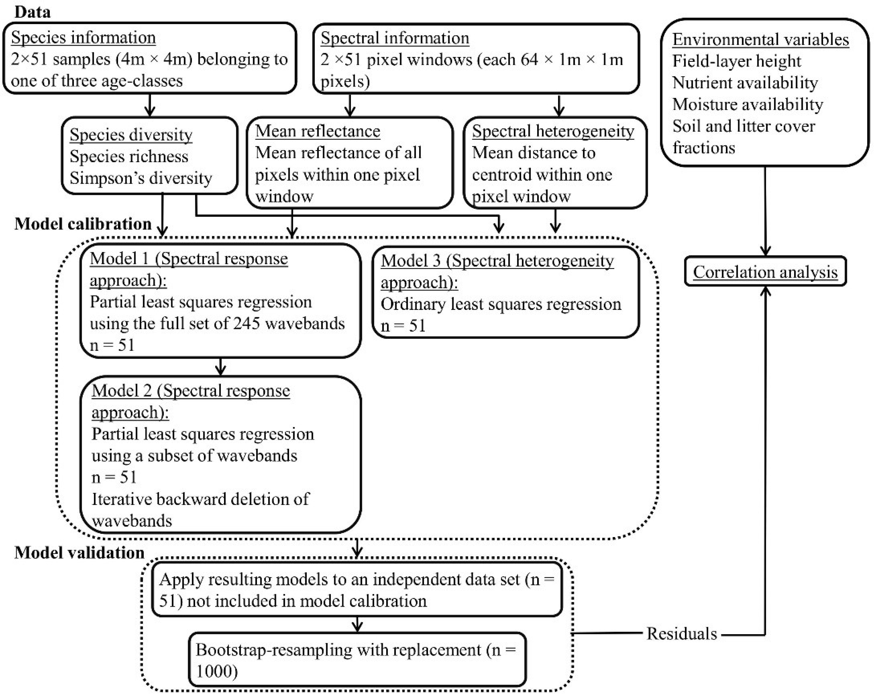
In the present study, we explore the ability of hyperspectral remote sensing technology to characterize fine-scale plant species diversity in dry, grazed grassland habitats in an agricultural landscape on the Baltic island of Öland (Sweden). We compare the performance of two modeling-based approaches to the prediction of species diversity in 4 m × 4 m plots, using data from airborne HySpex hyperspectral imagers (415–2345 nm). We ask the following questions: can hyperspectral data be used to predict the SR and iSDI in dry grazed grasslands via the direct relationship between reflectance data and field-based measures of plant species diversity using (1) an analysis of reflectance, based on information from (i) all wavebands; and (ii) a subset of wavebands, analyzed with a partial least squares regression model (hereafter referred to as the spectral response approach); and (2) an analysis of spectral heterogeneity, based on the mean distance to the spectral centroid in an ordinary least squares regression model (hereafter referred to as the spectral heterogeneity approach)? We also investigate whether the possible relationship between hyperspectral data and species diversity is influenced by environmental conditions (grazing continuity, nutrient and moisture status, field-layer height, and soil- and litter-cover fractions).

2. Materials and Methods

2.1. Study Area and Site Selection

The study area is located in the southeast of Sweden on the Baltic island of Öland (Figure 1a; centered on 56°40′49′′N, 16°33′58′′E) and covers approximately 22.5 km2. The bedrock consists mainly of Ordovician limestone, and the area is characterized by a generally flat topography (cf. [9]). The climate on the island is maritime (mean annual temperature: 7 °C, mean annual precipitation: 468 mm) (cf. [9]). The present-day landscape consists of a mosaic of arable fields, deciduous forest, villages and grazed grasslands; the majority of the grasslands are grazed by cattle at varying intensities. The grassland sites in the landscape represent different stages of succession—ranging from young grasslands on recently abandoned arable fields to grassland sites with a history of grazing of more than 280 years.
Figure 1. (a) The location of the study area on the Baltic Island of Öland, Sweden; (b) the distribution of grassland sites included in the present study (n = 52); (c) an example of the distribution of field plots within some of the grassland sites.
Remotesensing 08 00133 g001
A total of 299 grassland sites were identified within the study area, with the help of the most recent (2005) land-use map (B.C. Schmid, unpublished data) and field visits. An overlay analysis of land-use maps from different time periods was used to assign each of the grassland sites into one of three age classes within the arable-to-grassland succession (young grasslands: 5–14 years, intermediate-aged grasslands: 15–49 years, and old grasslands: ≥50 years of grazing management). The overlay analysis was based on land-use maps from 2005 (B.C. Schmid, unpublished data), 1994, 1959 and 1730 (cf. [9]). The land-use map from 2005 was developed from a digital color infrared aerial orthophoto (0.5 m pixel size) geometrically corrected with the help of a digital terrain model. The land-use maps from 1994 to 1959 were developed from aerial photos (1994: color infrared, 1959: black and white) at the scale of 1: 30,000. The land-use map from 1730 was based on a set of large-scale (1: 4000), high-quality survey maps from the early 18th century (cf. [9]).
Within each of the 299 sites, we randomly positioned two coordinate points in open (i.e., not covered by shrubs or trees) grassland vegetation with the constraints that they had to be at least 25 m apart, at least 13.5 m from the site boundary (to minimize edge effects in the vegetation), and at least 13.5 m from shrubs or trees that were higher than 50 cm (to minimize shading effects in the vegetation). A total of 239 out of the 299 grassland sites could accommodate these constraints. A hand-held differential global positioning system (GPS) receiver (Topcon GRS-1 GNSS, equipped with a PG-A1 external antenna; Topcon Corporation, Japan) was used to log the ground coordinates of the points.
Sixty sites (20 young, 20 intermediate, and 20 old) were randomly selected from the 239 sites. Within these 60 sites, a bioassay approach (cf. [23]) based on indicator species, such as Sesleria caerulea and Molinia caerulea, was used to identify sites with “dry” grassland vegetation, and to exclude moist grassland vegetation. A total of 52 sites (17 young, 18 intermediate, and 17 old) out of the 60 sites were characterized as dry grassland vegetation; these sites were used for the field-based vegetation and remote sensing sampling (Figure 1b).

2.2. Field Sampling

2.2.1. Vascular Plant Species Richness and Diversity

The fieldwork was carried out between 15 May and 15 July 2011. A 4 m × 4 m plot (divided into a grid of 16 sub-plots, each 1 m × 1 m), was centered over each of the two coordinate points, within each of the 52 chosen sites (Figure 1c). The presence of all non-woody vascular plants was recorded within each 1 m × 1 m sub-plot. The within-plot species diversity was characterized: (a) in terms of species richness (SR), calculated as the total number of vascular plant species present in a 4 m × 4 m plot and (b) in terms of the inverse Simpson diversity index (iSDI)
i S D I = 1 / i = 1 S p i 2
where S is the number of species in the plot and pi is the proportion of the ith species in a plot [24]. The inverse Simpson diversity index assigns a lower weight to rare species, thus emphasizing the most abundant species in the vegetation canopy [25]. Because the inverse Simpson diversity index characterizes the dominance structure of plant communities (which, in its turn, contributes to the spectral signal of vegetation canopies), it may be particularly informative in remote sensing studies [17]. From a statistical point of view, the number of species within a specific area represents discontinuous data, and thus has a Poisson or negative-binomial distribution. Because the partial least squares regression (PLSR) and ordinary least squares regression (OLSR) analyses used in the present study (Section 2.4) assume a normal distribution, we ln-transformed the SR values before analysis, so that the ln(SR) data approximate to a normal distribution. Ln(SR) and iSDI were calculated using the vegan package [26] in the R programming environment [27].

2.2.2. Environmental Variables

Each of the 4 m × 4 m plots was assigned values for the following environmental variables: grazing continuity, nutrient and moisture status, field-layer height, and soil- and litter-cover fractions (Table A1). Soil nutrient and moisture status were assessed indirectly, with the help of Ellenberg indicator values for nutrient (Ellenberg N) and moisture (Ellenberg M) availability [28]. For each of the sampled plant species, values for Ellenberg N and M were extracted from the JUICE database [29]. A community-weighted mean value (CWM) [30] was calculated for N and M within each plot:
C W M ( x ) = i p i × x i
where pi is the relative frequency of the ith species and xi is the Ellenberg indicator value of the ith species. The CWM for Ellenberg N (Ellenberg mN) and Ellenberg M (Ellenberg mM) were calculated using the FD package [31] in the R programming environment [27]. Field-layer height (cm) was estimated as the mean vegetation height at 100 points in the 1 m × 1 m sub-plot in the south-west corner of each 4 m × 4 m plot. Mean percentage covers of soil and litter fractions, respectively, for each of the 4 m × 4 m plots were based on the cover values (visually estimated by experienced field ecologists) within each of the 16 1 m × 1 m sub-plots.

2.3. Remote Sensing Data

2.3.1. Spectral Data Collection

Hyperspectral data were acquired by the company Terratec AS, Lysaker, at around solar noon on 9 July 2011. Two airborne HySpex hyperspectral imagers (Norsk Elektro Optikk, Lörenskog, Norway), VNIR-1600 and SWIR-320m-e, were used in the push broom scanning mode (Table A2). The flight altitude was approximately 1500 m and the weather conditions were cloud-free. A total of 25 flight lines (conducted either from north to south or from south to north, to minimize illumination effects) were recorded.

2.3.2. Preparation of Spectral Data

Wavebands between 962–985 nm, 1322–1496 nm, 1803–2050 nm, and 2351–2501 nm were deleted from the hyperspectral data set because of strong atmospheric interference or detector overlap, leaving 245 wavebands that were used for further analysis. ATCOR-4 software [32], which is based on the radiative transfer model MODTRAN 5 [33], was used for atmospheric and topographic corrections of the hyperspectral data. The atmospheric correction was carried out using the settings for rugged terrain, the desert aerosol model, a water vapor column of 1.0 g·m−2, visibility of 28.4 km, and an ozone concentration of 330 Dopson units. The radiance was converted into reflectance using the Fontenla-2011 solar irradiance spectrum [34]. The images were orthorectified with an accuracy of approximately 0.3 m, by the data providers, using the PARGE software [35]. To match the spatial resolution of the two HySpex sensors, the spectral data originating from the VNIR-1600 spectrometer were resampled to a spatial resolution of 1 m, using a triangulated nearest neighborhood method, and a spectral resolution of 6 nm, using locally weighted scatterplot smoothing (LOESS) interpolation [36]. High frequency noise in the spectral data was reduced by using a cubic Savitzky–Golay filter [37] with a kernel size of 21 nm. The resampling was done using the signal [38] and raster packages [39] and the filtering was done using hyperSpec package [40] in the R statistical environment [27].

2.3.3. Calculating Mean Spectral Reflectance and Spectral Heterogeneity

Vector polygons of the grassland sites were overlaid onto the hyperspectral imagery, and each individual 4 m × 4 m field plot was located on the HySpex image using the GPS coordinates taken during the field work. Although we used a GPS receiver with a high accuracy, GPS errors may exist. To account for possible positional uncertainties, a pixel window of 8 × 8 pixels (8 m × 8 m) was centered on each of the 4 m × 4 m field plots and the reflectance of each pixel (n = 64) within each pixel window from the 245 individual wavebands was extracted.
Prior to the spectral response analyses, the reflectance was log10(1/Rλ) transformed (where Rλ is the reflectance at each waveband). The mean transformed reflectance of each pixel window was obtained by calculating the mean spectral value of the pixels (n = 64) for each of the 245 individual HySpex wavebands. Log10(1/Rλ) transformed reflectance shows a near-linear relationship with the concentration of absorbing land surface components [41], and may provide important information on the environmental and ecological processes underlying any potential associations between hyperspectral data and plant species diversity [42].
Several different methods have been used to compute spectral heterogeneity in remotely sensed data. For example, Viedma [43] used methods based on spectral texture data, while Heumann [44] applied an approach using measures of statistical dispersion to represent spectral diversity. Warren [45] compared two categories of spectral heterogeneity metrics—one category calculated with the help of principle component analysis (PCA) and one category developed from semivariogram descriptors—and found that both types of metrics performed equally well as predictors of species diversity. Oldeland [17] and Rocchini [46] also used spectral heterogeneity calculated with the help of PCA to model species diversity. Following Oldeland [17] and Rocchini [46], we applied a PCA-based approach to calculate spectral heterogeneity. The PCA was conducted on the spectral data set (n = 245) within each pixel window consisting of 64 pixels, using untransformed reflectance data. The spectral heterogeneity was calculated as the mean of the Euclidean distances between each of the 64 pixels and the centroid of the pixel-cloud within the PCA space using the first five principal components, which summarized at least 97% of the total spectral variation. We predicted that increasing within-plot environmental heterogeneity should be accompanied by an increasing mean distance to the spectral centroid (see [17,46]).

2.4. Data Analysis

The 104 plots were divided into a calibration subset and a validation subset by randomly assigning the two plots from each of the 52 grassland sites to one or other of the two subsets (Figure 1c). Two plots (one each from the calibration and validation subset) that had an unusually low reflectance in the spectral range 900–1300 nm were excluded from further analyses. The exclusion of the two plots resulted in a total of 102 plots (51 plots in each subset) used for the data analysis (Figure 2).
Figure 2. Schematic overview of the workflow used in the present study.
Remotesensing 08 00133 g002
The Pearson correlation between the species diversity indices (ln(SR) and iSDI) and the mean spectral reflectance of each pixel window for individual wavebands were analyzed for all plots (n = 102). In the spectral response approach, the relationships between hyperspectral data and field-observed ln(SR) and iSDI were investigated for the plots in the calibration subset, using “leave-one-out” cross-validated PLSR of (i) the full set of 245 (Model 1) and (ii) a subset (Model 2) of HySpex wavebands (Figure 2). Earlier studies showed that the exclusion of wavebands that provide little information related to the response variable improves the PLSR-based prediction of vegetation variables [47]. We used iterative variable deletion to identify the wavebands used in Model 2 (i.e., the bands most important for prediction of species diversity). Marten’s uncertainty test [48] and the variable importance in projection (VIP) values [49] were calculated for each waveband to identify the least important wavebands (variables) within each iterative step. Variables that were non-significant and had a VIP value lower than 0.8 were deleted before recalibrating the model. This procedure was repeated until none of the remaining variables could be deleted. The relationships between hyperspectral data and field-observed species diversity were also examined using spectral heterogeneity and OLSR analysis (Model 3) (Figure 2). The validation subset was used to evaluate the regression models of the calibration subset.

2.4.1. Partial Least Squares Regression Analysis (PLSR)—Models 1 and 2 (Spectral Response Approach)

A PLSR analysis [49] between each of the two diversity indices (dependent variables) and the average spectral reflectances (explanatory variables) was carried out. PLSR is a method of multivariate analysis that is suitable for the analysis of data sets that include a larger number of (highly correlated) explanatory variables than samples [50]—which is often the case in remote sensing–based species diversity studies. Several studies have shown that the PLSR method outperforms other methods (e.g., OLSR) when analyzing highly co-linear hyperspectral remote sensing data sets [51]. The PLSR algorithm attempts to find latent variables (LVs) that summarize the variation in the explanatory matrix and, at the same time, maximize the covariance with the dependent variable (see [52]).
The optimal number of LVs needs to be identified in order to avoid model over-fitting in PLSR analyses, but there is, at present, no consensus about the best method to use [53]. The number of LVs is usually determined by a cross-validation procedure, which is used to find the lowest cross-validated root mean square error (RMSECV) of the PLSR model. It has been shown that the use of the global minimum of the RMSECV can lead to erroneous and over-fitted prediction models [53]. To avoid over-fitting, the first local minimum of the RMSECV is usually used [54]. However, this approach may lead to model under-fitting, if the minimum error results in a negative coefficient of determination for the cross-validated predicted dependent variables (R2CV). Negative values of R2CV indicate that the model residuals exceed those obtained from the mean observation as predictors. We used the number of LVs which resulted in the first local minimum absolute RMSECV (aRMSECV) and a positive R2CV value. To allow comparison between Models 1 and 2, we normalized the aRMSECV (nRMSECV, %) values by the range of the field-observed values for ln(SR) and iSDI of the calibration subset.
The PLSR was run in two ways: (i) using all wavebands from the full reflectance spectrum (n = 245; Model 1); and (ii) using the subset of spectral wavebands that were most important for the prediction of species diversity (Model 2). Cross-validation was carried out using “leave-one-out” cross-validation, with each plot being excluded in turn, and the calibration model based on the remaining plots used to predict the excluded plot. Both the models (Model 1 and Model 2) for each of the two species diversity indices were validated with the plots from the independent validation subset. The root mean square error of the predicted values (absolute value: aRMSEP) and the squared correlation coefficient (R2P) between the field-observed and predicted ln(SR) and iSDI for the validation subset were used to evaluate the predictive qualities of the models. The aRMSEP was normalized (nRMSEP, %) by the range of the field-observed ln(SR) and iSDI values of the validation subset. A good validation result is characterized by low values for both aRMSEP and nRMSEP and high values for R2P, indicating that the hyperspectral data have a good ability to predict the species diversity indices. To assess the robustness of the predictive performance of the calibrated PLSR models, the validation subset was bootstrapped 1000 times (with replacement), building 1000 “new” validation subsets. The calibration model was applied to each of the 1000 validation subsets and the nRMSEP (%) and R2P between the field-observed and predicted ln(SR) and iSDI were calculated for each validation subset. Mean nRMSEP (%) and R2P values, and 95% confidence levels were then calculated for the 1000 validation subsets.

2.4.2. Residual Analysis of Models 1 and 2 (Spectral Response Approach)

The residuals of Models 1 and 2 were separately correlated with the environmental variables Ellenberg mN and mM, field-layer height, bare ground and litter-cover fractions (Table A1), to examine whether the relationships between hyperspectral data and species diversity was influenced by the environmental variables characterizing the plots. The significance of the correlations was tested using a two-sided Student’s t-test. Because multiple tests may result in an increased risk of Type I error, the significance values of the correlations were assessed after Bonferroni correction. To investigate whether the relationships between hyperspectral data and species diversity were influenced by the age-class of plots (young grasslands: 5–14 years, intermediate-aged grasslands: 15–49 years, and old grasslands with ≥50 years of grazing continuity), we examined if there were significant differences between the residuals associated with each of the three grassland age-classes. Because the residuals were not normally distributed we used the Kruskal-Wallis test [55]. All analyses were conducted in the R statistical environment [27], using the pls package [54].

2.4.3. Ordinary Least Squares Regression Analysis (OLSR) and Reduced Major Axis Regression—Model 3 (Spectral Heterogeneity Approach)

Previous studies successfully applied OLSR to examine the relationship between spectral heterogeneity and plant species diversity [17]. In the present study, separate OLSR analyses of the relationships between each of the species diversity indices (dependent variables) and the spectral heterogeneity (explanatory variable) were carried out on the calibration subset (Model 3) (Figure 2). Model 3 was tested on the validation subset using a reduced major axis (RMA) regression. Curran [56] showed that RMA is an appropriate method for the remote sensing–based prediction of grassland variables, in cases where there is no available information on measurement error. The nRMSEP and R2P were used to evaluate the performance of the validation.

3. Results

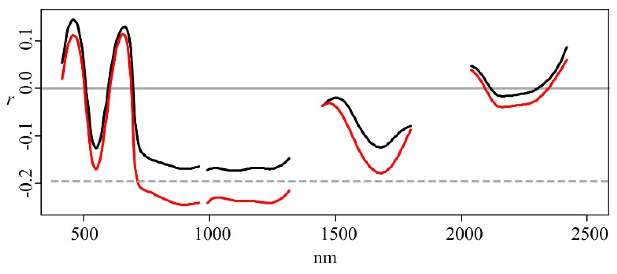
The summary statistics for the dependent variables for the plots within each grassland age-class (young, intermediate-aged, and old grasslands) are presented in in Table A3. The Pearson’s correlation coefficients between the ln(SR) and the iSDI were significant for both the calibration (r = 0.98, p < 0.001) and validation subsets (r = 0.97, p < 0.001). There were significant negative correlations (p < 0.05) between the reflectance associated with wavebands in the near-infrared (758–1316 nm) (NIR) part of the electromagnetic spectrum and the ln(SR) (Figure 3). There were positive but non-significant correlations between the reflectance at wavebands in the blue (415–499 nm) and red (602–752 nm) parts of the spectrum and the dependent variables, and (non-significant) negative correlations between the reflectance at wavebands in the green (505–595 nm) and SWIR (1502–2345 nm) parts of the spectrum and the dependent variables (Figure 3).
Figure 3. Pearson’s correlation coefficients (r) between single wavebands and the species richness ln(SR) (red), and the inverse Simpson’s diversity index iSDI (black) for the whole data set (n = 102). Correlations below the dotted line are significant (p < 0.05).
Remotesensing 08 00133 g003

3.1. Spectral Reflectance—Models 1 and 2 (Spectral Response Approach)

3.1.1. PLSR Using the Full Set of 245 HySpex Wavebands—Model 1

The inclusion of seven LVs gave the first local minimum absolute aRMSECV in the PLSR model developed from the calibration subset (Model 1; Figure 2), for both the ln(SR) (aRMSECV = 0.34) and the iSDI (aRMSECV = 8.87) (Table 1).
Table 1. Summary of the ability of PLSR models, based on spectral reflectance using the full set of wavebands (Model 1) or a subset of wavebands (Model 2), to predict the species richness (ln(SR)) and the inverse Simpson’s diversity index (iSDI). The cross-validated error of the calibration models (n = 51) is indicated by the absolute (aRMSECV) and normalized RMSECV (nRMSECV, %). LV indicates the number of latent variables used in the PLSR models. The absolute and normalized prediction errors (aRMSEP, nRMSEP (%)) indicate the ability of the model to predict the observed species diversity measure. The squared correlation (R2P) indicates the fit between the predicted and observed diversity values from the validation subset (n = 51).
aRMSECVnRMSECVLVaRMSEPnRMSEPR2PNo. of Wavebands
ln(SR)Model 10.3421%70.2919%0.43245
Model 20.3723%50.3422%0.1925
iSDIModel 18.8723%76.7720%0.45245
Model 29.2925%47.0721%0.4035
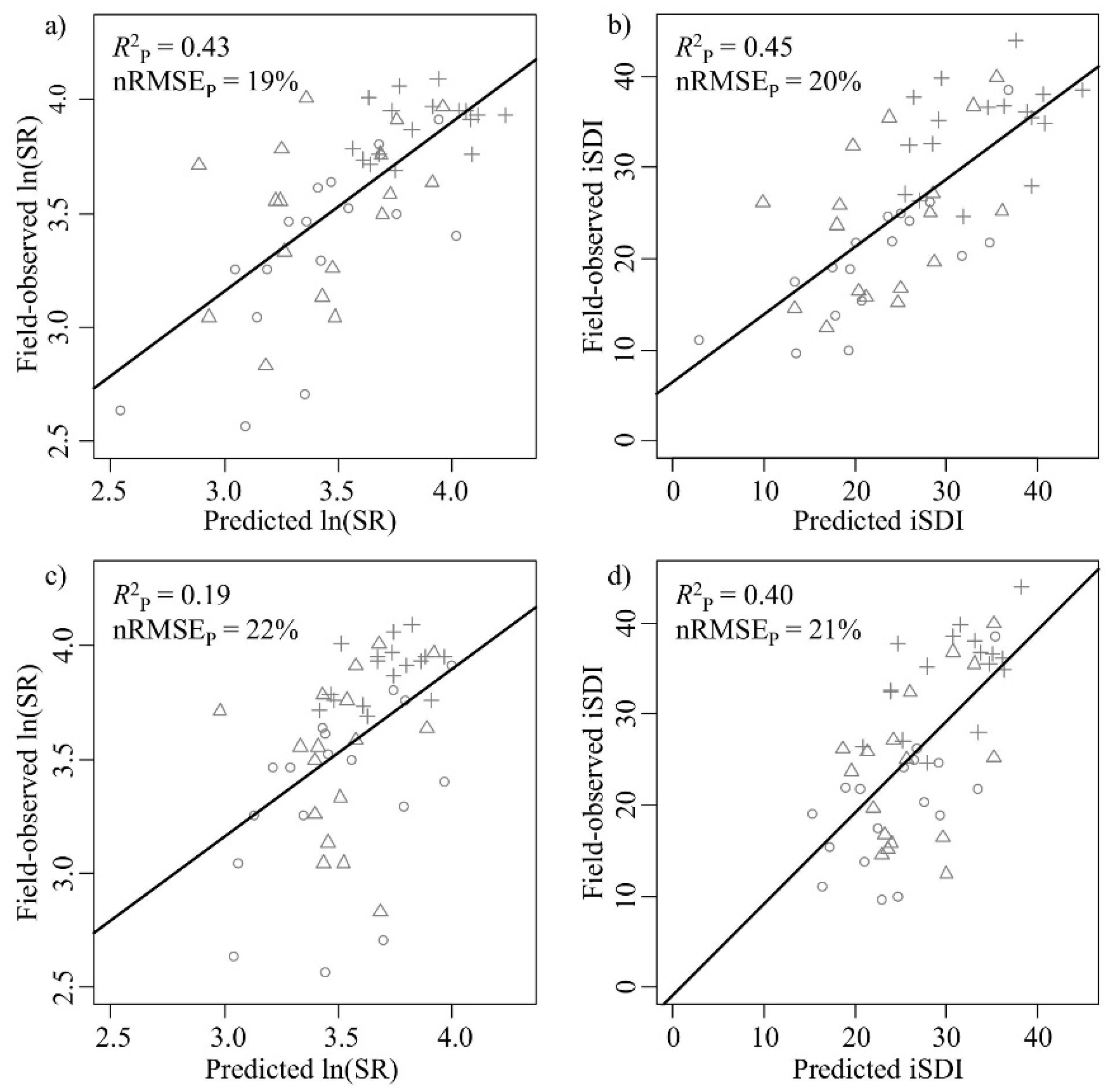
The correlations between the field-observed and predicted measures of species diversity were significant for both the ln(SR) (R2P = 0.43, p < 0.001) and the iSDI (R2P = 0.45, p < 0.001) (Table 1, Figure 4a,b). The nRMSEP values were approximately 20% for both the ln(SR) (nRMSEP = 19%) and the iSDI (nRMSEP = 20%) (Table 1, 
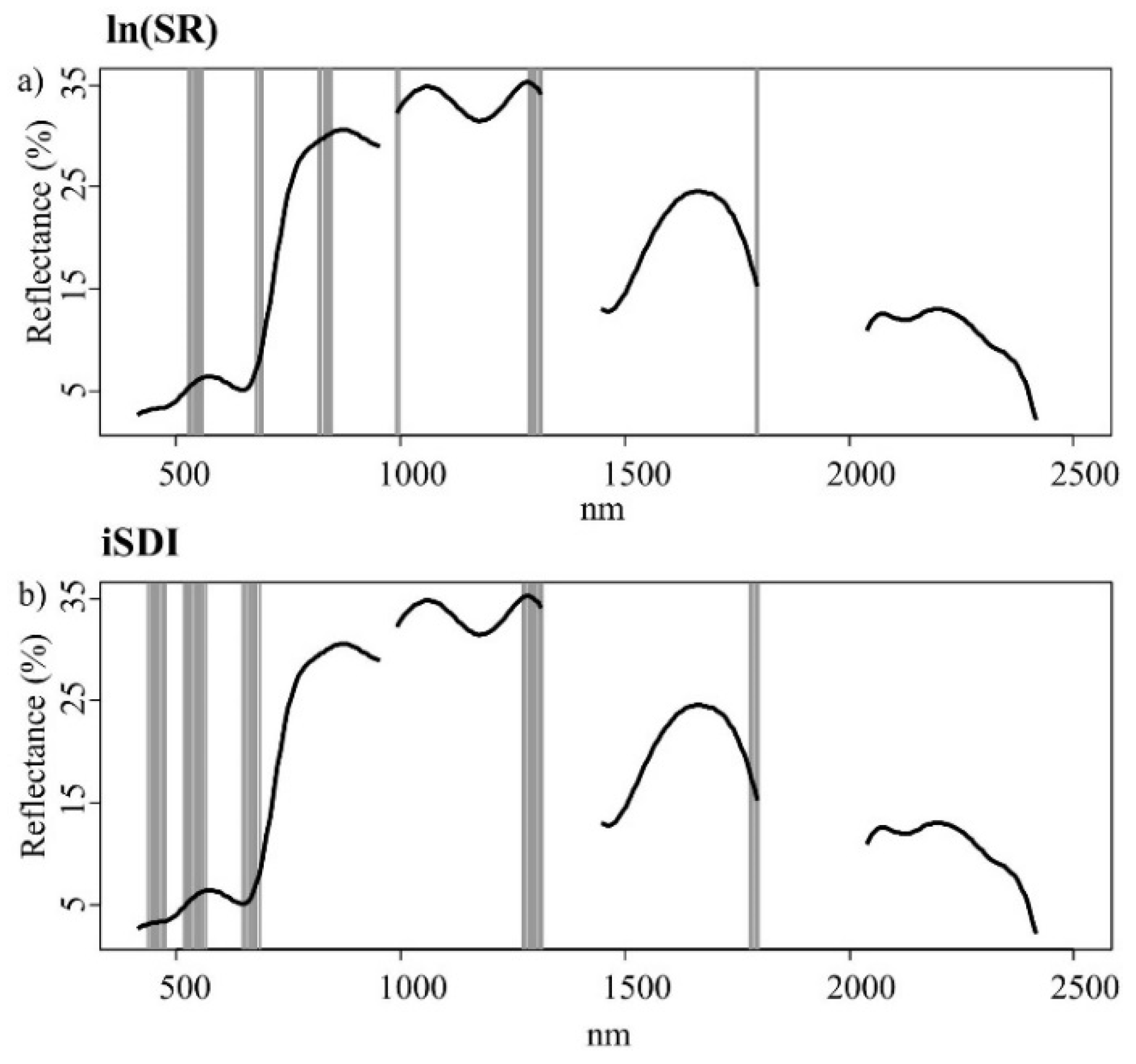
Figure 4a,b). Out of the 245 wavebands used in Model 1, 25 bands were most important for the prediction of the ln(SR) (Figure 5a, Table A4), while 35 bands were most important for the prediction of the iSDI (Figure 5b, 
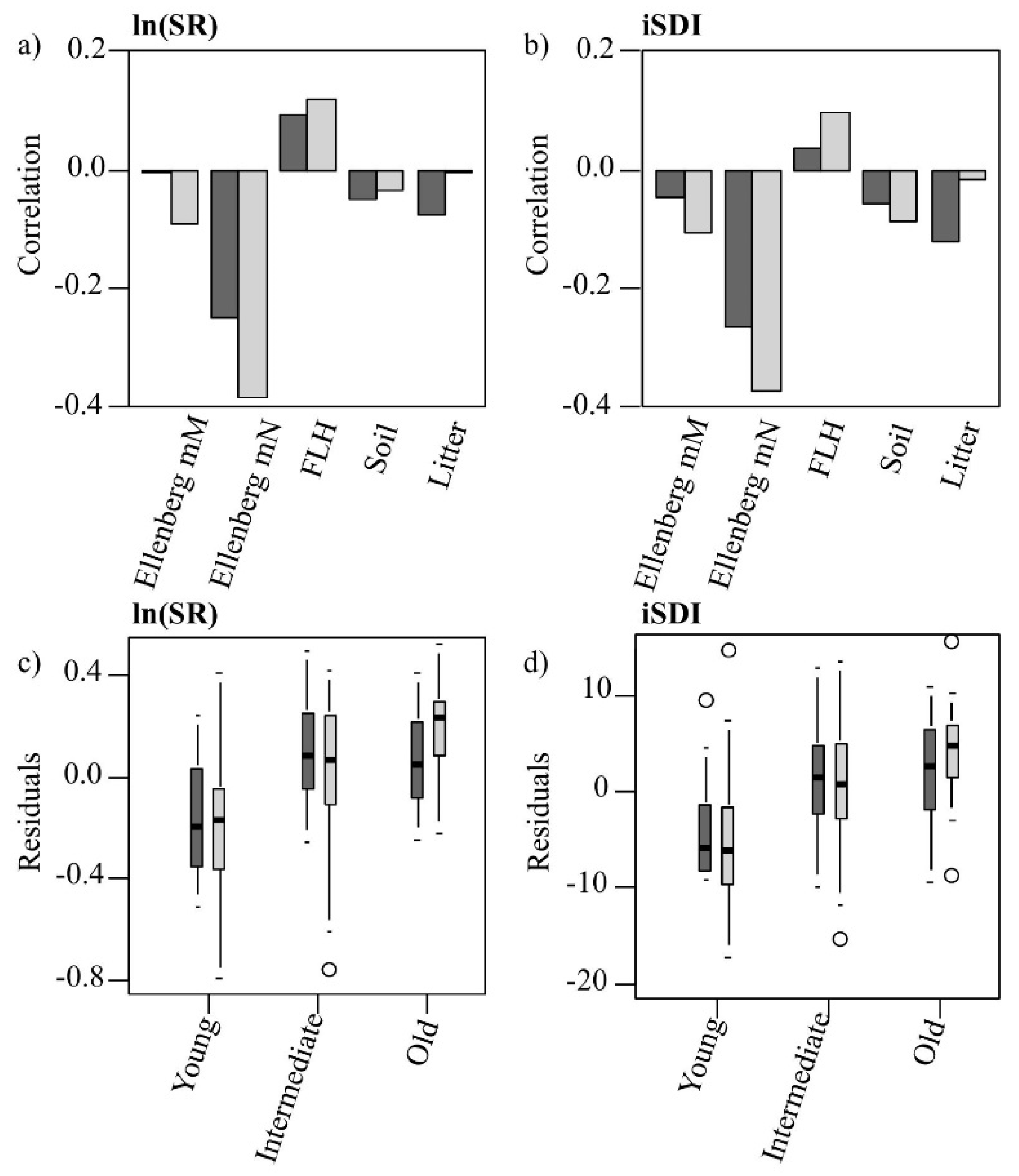
Table A4). The relationships between the residuals associated with the prediction of both dependent variables (using Model 1) and the values for individual environmental variables (Ellenberg mN and mM, field-layer height, and soil- and litter-cover fractions) were non-significant (Figure 6a,b). There were significant (p < 0.05), positive associations between the residuals (in the prediction of both the ln(SR) and the iSDI) and the grassland age: the shorter the grazing continuity of the grassland, the more the values for ln(SR) and iSDI were overestimated (negative residuals) (Figure 6c,d).
Figure 4. Correlations between field-observed and predicted (left column) species richness (ln(SR)) and (right column) inverse Simpson’s diversity (iSDI) for the validation subset (n = 51). (a,b) show the field-observed versus the predicted correlations for the PLSR model based on the full set of wavebands (Model 1) (n = 245); (c,d) show the field-observed versus the predicted correlations for the model based on a subset of wavebands (Model 2) (n = 25 (for ln(SR)) or 35 (for iSDI)). The normalized prediction error (nRMSEP, %) indicates the quality of the model in predicting the observed species diversity measure, and the squared correlation (R2P) indicates the fit between the predicted and observed diversity value. The age-class of the grassland plots is also displayed (key: ○ young, ∆ intermediate, and + old). Black lines indicate the relationship between the predicted and the measured values.
Remotesensing 08 00133 g004
Figure 5. Important wavebands (grey bars) selected with the help of an iterative variable deletion procedure, for estimating (a) the species richness (ln(SR)) and (b) the inverse Simpson’s diversity index (iSDI) in grassland plots using the calibration subset (n = 51). The black line represents the mean spectral reflectance curve for grassland plots in the whole data set (n = 102).
Remotesensing 08 00133 g005
Figure 6. (a,b) Pearson’s correlation coefficients of the residuals of the PLSR models’ (Model 1 = dark; Model 2 = light) predictions of (a) the species richness (ln(SR)) and (b) the inverse Simpson’s diversity index (iSDI) with different environmental variables (moisture availability, Ellenberg mM; nutrient availability, Ellenberg mN; field-layer height, FLH; cover of bare ground, Bare ground; and cover of litter, Litter); (c,d) Distribution of the residuals of (c) the species richness (ln(SR)) and (d) the inverse Simpson’s diversity index (iSDI), within the three grassland age-classes, predicted by Model 1 (dark) and Model 2 (light).
Remotesensing 08 00133 g006

3.1.2. PLSR Using the Subset of HySpex Wavebands—Model 2

Using the subsets of HySpex wavebands (Model 2; Figure 2), the inclusion of five LVs gave the first local minimum aRMSECV in the PLSR model for ln(SR) (aRMSECV = 0.37) (Table 1). For the prediction of iSDI, the inclusion of four LVs gave the first minimum aRMSECV (aRMSECV = 9.29) (Table 1). The correlations between the field-observed and predicted measures of plant diversity for the validation subset were significant for ln(SR) (R2P = 0.19, p < 0.001) and iSDI (R2P = 0.40, p < 0.001) (Table 1, Figure 4c,d). The nRMSEP values were above 20% for ln(SR) (nRMSEP = 22%) and iSDI (nRMSEP = 21%) (Table 1, Figure 4c,d). In the Model 2 approach, there were significant negative correlations (p < 0.05) between the residuals (associated with the prediction of ln(SR) and iSDI) and the Ellenberg mN: the higher the Ellenberg mN, the more the values for ln(SR) and iSDI were overestimated (negative residuals) (Figure 6a,b). There were also significant (p < 0.05) associations between the residuals (in the prediction of ln(SR) and iSDI) and the grassland age: the shorter the grazing continuity of the grassland, the more the values for ln(SR) and iSDI were overestimated (negative residuals) (Figure 6c,d).

3.1.3. The Robustness of the Prediction Models (Models 1 and 2)

The bootstrapping procedure revealed that the mean R2P were higher and the mean nRMSEP were lower when using the PLSR-based models developed from the full set of bands (Model 1) than when using the models developed from the subset of bands (Model 2) to predict both the dependent variables (Table 2).
Table 2. Bootstrap results showing the ability of the PLSR models based on the spectral reflectance in the full set of wavebands (Model 1) and the subset of wavebands (Model 2) to predict the species richness (ln(SR)) and the inverse Simpson’s diversity index (iSDI). Mean R2P and mean nRMSEP (%) are the average squared correlation coefficients and normalized prediction errors for the validation subset, based on 1000 bootstraps. The 95% confidence limit indicates the upper and lower confidence intervals of the mean values.
Mean R2P95% Confidence LimitMean nRMSEP95% Confidence Limit
ln(SR)Model 10.39±0.01020%±0.1%
Model 20.17±0.00923%±0.1%
iSDIModel 10.43±0.00821%±0.1%
Model 20.38±0.00722%±0.1%

3.2. Linear Regression Based on Spectral Heterogeneity—Model 3 (Spectral Heterogeneity Approach)

When the regression models (Model 3; Figure 2) developed from the calibration subset using the spectral heterogeneity approach were applied to the validation subsets, the results showed non-significant relationships between both the field-observed and predicted SR (R2 = 0.06, p > 0.05) and the field-observed and predicted iSDI (R2 = 0.04, p > 0.05). The nRMSEP values were above 30% for both ln(SR) (nRMSEP = 31%) and iSDI (nRMSEP = 35%).

4. Discussion

4.1. The Relationship between Hyperspectral Reflectance Measurements and Plant Species Diversity (Spectral Response Approach—Models 1 and 2)

The spectral response approach, using both Model 1 and Model 2, resulted in good predictions, with a relative error (nRMSEP) of approximately 20% of both ln(SR) and iSDI (Figure 4, Table 1 and Table 2). PLSR-based approaches have been used in the past to predict plant species diversity in grassland ecosystems with the help of hyperspectral remote sensing [18,19]. The study by Fava [18] used ground-based hyperspectral measurements and PLSR to assess plant species diversity (species richness and Shannon diversity) in alpine meadow systems and showed a somewhat lower average error (<15%) for the plant diversity estimates than was found in the present study. The relatively higher error values in the present study may reflect the fact that airborne spectrometric measurements are affected by noise caused by, for example, effects of atmospheric scattering. Carter [19] used airborne spectrometric measurements (400–2500 nm) to estimate species richness in mesic grasslands, and revealed somewhat weaker relationships between the spectral data and species diversity than those in the present study. The analyses in Carter [19] were based on simple linear regression using individual wavebands and band ratios, whereas our analyses used a PLSR-based approach involving multiple bands. The use of a limited number of wavebands may result in poorer relationships between remote sensing data and vegetation parameters compared with the use of many spectral bands. Although much information in a hyperspectral data set may be redundant, important spectral information may nevertheless be lost when only a small number of wavebands are used to predict vegetation variables [57].

4.2. The Most Important Hyperspectral Wavebands for Predicting Plant Species Diversity Using the Spectral Response Approach (Models 1 and 2)

Previous studies revealed that the soils of young grasslands with a short history of grazing management often contain high levels of nitrogen and phosphorus as a result of their recent use as fertilized arable fields [58]. Over time, the continuous removal of above-ground biomass by grazing animals leads to a progressive decrease in soil nutrient levels [58]. Nutrient-poor conditions promote the maintenance and establishment of plant species with a low competitive ability. Grasslands with a long grazing continuity, such as the old grasslands in our study (Table A3), are often associated with a lower above-ground biomass and a higher plant species diversity than young grasslands [59,60]. An increase in the amount of above-ground biomass is often accompanied by an increase in the reflectance in the NIR region of the spectrum because of increased multiple scattering within the canopy (e.g., [61]). Relationships between species richness and above-ground biomass have been extensively studied (e.g., [12]) and have increasingly been used to interpret the relationship between reflectance and species diversity measures in grasslands (e.g., [18,62]. For example, [18] explained the relationship between reflectance in the NIR wavebands and species richness in terms of a negative relationship between biomass and plant diversity. In the present study, the identification of key wavebands for predicting species diversity in the PLSR models 1 and 2 showed that several NIR wavebands were important for the assessment of species diversity (Figure 5). Significant negative correlations between reflectance and diversity in the NIR spectral region (Figure 3) indicate that the species diversity increased as the above-ground biomass decreased. Other studies have shown that the visible wavebands may also contain important information for the assessment of plant species richness (e.g., [18]). The relationships we identified between wavebands in the visible and SWIR parts of the spectrum and the species diversity are in line with those findings (Figure 5). The positive associations that we observed between reflectance and diversity in the chlorophyll absorption regions of the spectrum (blue and red) and the negative associations with the green and the water absorption parts (SWIR bands) of the spectrum (Figure 3) suggest that the species-poor plots were characterized by higher levels of plant chlorophyll content and vegetation water content than the species-rich plots.

4.3 Residual Analysis of Models 1 and 2 (Spectral Response Approach)

The lack of significant relationships between the residuals of Model 1 and the environmental variables indicates that none of these variables had an effect on the species diversity that was not predicted by the full set of hyperspectral wavebands (Figure 6a,b). In contrast, the significant relationships between the residuals for Model 2 and nutrient status suggest that the unexplained variance in the models based on a subset of wavebands may be related to within-plot soil nutrient availability (Figure 6a,b). In the present study, the use of a subset of wavebands (Model 2) may have resulted in the loss of spectral information on the variation in nutrient status, which may, at least partly, explain the poorer prediction of species diversity in Model 2 compared with that for Model 1 (Figure 4, Table 1 and Table 2).
For both Model 1 and Model 2, the residuals differed significantly between the age-classes, indicating that the unexplained variance was related to the grazing continuity within the plots (Figure 6c,d). Thus, in Model 1 and Model 2, the grazing continuity had effects on the species diversity that were not predicted from the spectral data. Although young grasslands are often associated with higher amounts of above-ground biomass and lower species diversity than old grasslands [60], the current grazing intensity is expected to influence the amount of biomass within the grasslands. Some of the young grassland sites may be subject to relatively high grazing intensity, and thus be characterized by a relatively low amount of above-ground biomass, which may explain the overestimation of the predicted species diversity in some of those plots (Figure 4). The overestimation of ln(SR) in low ln(SR) plots tended to be more accentuated in the Model 2 approach than in the Model 1 approach (Figure 4a,c). The full set of wavebands may include individual bands that were important for the prediction of particular (heavily grazed) low ln(SR) plots—and these bands were excluded in the backward deletion procedure which may explain the poorer R2 value in Model 2 than in Model 1. A higher number of wavebands were retained in Model 2 for the iSDI response variable than for the ln(SR) variable, and there was little difference between the Model 1 and Model 2 results for iSDI (Figure 4b,d). Although the number of LVs may not always be a good measure of model complexity [63], the lower number of LVs in the Model 2 analyses (Table 1) indicate that the Model 2 analyses were more parsimonious than the Model 1 analyses.

4.4. The Relationship between Spectral Heterogeneity and Plant Species Diversity (Spectral Heterogeneity Approach—Model 3)

Relationships between spectral heterogeneity and measures of species diversity have been investigated in recent studies [17,46]. However, these studies were carried out at relatively coarse spatial scales (sampling areas ≥100 m2) [17,46]. Large sampling areas may be characterized by a greater variability in the environmental conditions than smaller areas (cf. [64]), and the strength of the relationship between spectral heterogeneity and plant species diversity has been shown to increase with the size of the spectral and vegetation sampling areas [43]. In the present study, spectral heterogeneity failed to predict species diversity within our comparatively small (4 m × 4 m) vegetation plots. Whereas our study was based on a pixel size of 1 m, previous studies of patterns of plant species co-existence within the same study area revealed heterogeneity in the plant community composition at a scale of decimeters rather than meters [65]. The failure to detect a significant relationship between spectral variability and species diversity in our study is, therefore, likely to reflect the fact that the scale (dictated by the pixel size) at which we worked was too large to detect ecologically relevant heterogeneity in the grassland community composition.

4.5. Limitations

One possible explanation for the discrepancy between the field-observed and predicted species diversity, in both the spectral response approach and the spectral heterogeneity approach, may be the mismatch between the size of the pixel windows (8 m × 8 m) and the size of the vegetation plots (4 m × 4 m). Although the paired spectral and vegetation plots belong to the same grassland age categories, and there is no variation in grazing intensity between the spectral plot and its corresponding vegetation plot, we cannot exclude the possibility that the relationship may have been influenced by environmental conditions in the 2 m zone surrounding the vegetation plots. However, species diversity levels at different spatial scales often show a positive relationship within semi-natural grasslands (e.g., [66,67]). For example, within Swedish semi-natural grassland the species diversity at the 1 dm × 1 dm scale was explained by the size of the species pool at the 2 m × 2 m scale [66].

5. Conclusions

The monitoring of biodiversity is regarded as a central task for nature conservation, and hyperspectral remote sensing has recently been identified as a method that has the potential to make a substantial contribution to the mapping of habitat and species diversity at local to regional scales [68]. The present study presents a novel methodology for the assessment of fine-scale (4 m × 4 m) vascular plant species diversity in dry grasslands based on hyperspectral data obtained with the help of airborne spectrometers covering 414 to 2501 nm. We used two different approaches to evaluate the ability of hyperspectral measurements to predict fine-scale grassland species diversity (characterized with the help of the species richness (SR) and the inverse Simpson’s diversity index (iSDI)). The spectral response approach included information on reflectance based on (i) all wavebands (Model 1), and (ii) a subset of wavebands (Model 2), input into a partial least squares regression (PLSR) model. The spectral heterogeneity approach was based on the spectral variation hypothesis, and included an analysis of spectral variation, based on the mean distance to the spectral centroid, in an ordinary least squares regression model (Model 3).
Our study demonstrates that a spectral response approach using airborne hyperspectral data can be used to predict fine-scale species diversity in dry grasslands. The relationships between the field-observed and predicted measures of plant species diversity were significant for both the SR and the iSDI with a normalized root mean square error of approximately 20% for the predicted values of both the diversity indices. The PLSR-based approach allows a large number of hyperspectral wavebands to be compressed into a few latent variables (LVs) while decreasing the risk of model overfitting. Although the average prediction quality for both SR and iSDI was poorer for the Model 2 procedure than for the Model 1 procedure, the lower number of LVs in the Model 2 analyses indicated that the Model 2 analyses were more parsimonious. The prediction quality of the PLSR algorithm is dependent on the optimal selection of LVs used in the final prediction model. Although there are different ways of selecting LVs, there has been no systematic comparison of the performance of the different approaches. We suggest, therefore, that alternatives to the first-local-minimum rule—such as the total minimum cross-validated error or an overall F-test of the loss function [53]—should be evaluated further in future studies. There was a negative correlation between the reflectance in the NIR spectral region and species diversity, indicating that the species diversity increased as the above-ground biomass decreased. Although the prediction errors of the two PLSR models derived from the spectral response approach are low for both the species diversity indices, a certain amount of variation within the predicted diversity indices remained unexplained in our study. We suggest that the unexplained variance in the predicted species diversity may, at least in part, result from between-site variation in grazing intensity (particularly in the younger grasslands on recently abandoned arable fields) that results in between-site differences in the amount of biomass.
The spectral heterogeneity approach, using spectral variability as a proxy for habitat heterogeneity, was unable to predict species diversity. Our results, together with results from earlier ecological studies [65], suggest that the relevant scale for the investigation of the relationships between environmental heterogeneity and fine-scale grassland species diversity in our study system may be smaller than the 1 m × 1 m pixels used in the study. We suggest that future studies should examine a wide range of pixel sizes to identify the scale, or scales, at which a relationship between environmental heterogeneity and species diversity can be identified.
In the present study, we used remotely sensed data acquired at a single time-point in July. If leaf senescence in response to summer drought is associated with lowered levels of spectral variation within and between the grassland plots, then a multi-temporal approach might improve the ability to predict grassland species diversity with the help of remotely sensed data. The use of unmanned aerial vehicles (UAVs), which can provide high levels of both spatial and temporal resolution, is attracting increasing attention within the field of fine-scale remote sensing (e.g., [44,68]). Future studies should examine the potential use of UAVs to deliver improved spectral data that can be used in the assessment of grassland species diversity.

Acknowledgments

We thank Sofia Pallander, Andreas Press and Johan Rydlöv for field assistance. We are grateful to Oskar Löfgren, Heather Reese, Duccio Rocchini and Susanne Thulin for their helpful comments on an earlier version of the manuscript. The research station “Station Linné” at Ölands Skogsby was used as a base for the fieldwork. We are grateful to the anonymous reviewers for their valuable comments on an earlier version of the manuscript.The study is a contribution to the Lund University Strategic Research Area “Biodiversity and Ecosystem Services in a Changing Climate” (BECC). The study was financed by grants from The Swedish Research Council for Environment, Agricultural Sciences and Spatial Planning (FORMAS) to Karin Hall and Honor C. Prentice.

Author Contributions

T.M., J.D., B.C.S., H.C.P. and K.H. planned and participated in the field work. T.M., J.D. and K.H. planned the collection of remotely sensed data. B.C.S. processed the land-use maps into a time-classified land-use map. T.M. processed and analyzed the data. All authors were involved in the research design, the interpretation of results, and the preparation of the manuscript.

Conflicts of Interest

The authors declare no conflict of interest.

Appendix A

Table A1. Mean values and standard deviations (stdev) for the environmental variables, measured in 4 m × 4 m plots belonging to the validation subset (n = 52).
Environmental VariablesMeanStdev
Ellenberg M3.550.53
Ellenberg N3.570.84
Field-layer height (cm)3.564.00
Soil-cover (%)6.138.18
Litter-cover (%)7.2917.01
Table A2. Technical characteristics of spectral sensors used in the study.
VNIR SensorSWIR Sensor
Sensor nameVNIR-1600SWIR-320m-e
Spectral coverage (nm)415–992967–2501
Spectral sampling interval (nm)3.76.0
Spectral bands160256
Field of view (FOV)1713.5
Ground sampling distance (m)0.51.0
Radiometric resolution (bit)1214
Table A3. Summary statistics for the ln-transformed species richness ln(SR) and the inverse Simpson’s diversity index (iSDI) values within the calibration and validation subsets for the 4 m × 4 m plots within each of the three grassland age-classes (young, intermediate-aged and old grasslands). The five most abundant species recorded within each grassland age-class are also presented.
ln(SR)iSDIFive Most Abundant Species
MeanStdevMinMaxMeanStdevMinMax
YoungCalibration (n = 16)3.280.412.644.2319.419.6610.1047.97Taraxacum agg., Dactylis glomerata, Poa pratensis, Lolium perenne, Convolvulus arvensis
Validation (n = 17)3.340.402.563.9120.007.139.6838.60
IntermediateCalibration (n = 18)3.590.332.894.1725.707.7313.4944.14Poa pratensis, Dactylis glomerata, Taraxacum agg., Festuca rubra, Ranunculus bulbosus
Validation (n = 17)3.510.352.834.0124.038.4412.4239.95
OldCalibration (n = 17)3.870.183.474.1134.496.0520.6343.21Plantago lanceolata, Galium verum, Achillea millefolium, Ranunculus bulbosus, Poa pratensis
Validation (n = 17)3.890.123.694.0934.385.2424.6243.97
Table A4. Number of important wavebands selected with the help of an iterative variable deletion procedure, for predicting the ln-transformed species richness ln(SR) and the inverse Simpson’s diversity index (iSDI) in grassland plots using the calibration subset (n = 51).
ln(SR)iSDI
Number of WavebandsPart of the Electromagnetic SpectrumNumber of WavebandsPart of the Electromagnetic Spectrum
6Green (529–559 nm)7Blue (439–475 nm)
3Red (680–692 nm)9Green (517–565 nm)
14NIR (818–1316 nm)7Red (650–686 nm)
2SWIR (1791, 1797 nm)8NIR (1274–1316 nm)
4SWIR (1779–1797 nm)

References

  1. Habel, J.; Dengler, J.; Janišová, M.; Török, P.; Wellstein, C.; Wiezik, M. European grassland ecosystems: Threatened hotspots of biodiversity. Biodivers. Conserv. 2013, 22, 2131–2138. [Google Scholar] [CrossRef]
  2. Gould, W. Remote sensing of vegetation, plant species richness, and regional biodiversity hotspots. Ecol. Appl. 2000, 10, 1861–1870. [Google Scholar] [CrossRef]
  3. Council of the European Union. Council Directive 92/43/EEC of 21 May 1992 on the Conservation of Natural Habitats and of Wild Fauna and Flora. Available online: http://eur-lex.europa.eu/legal-content/EN/TXT/?uri=CELEX%3A31992L0043 (accessed on 2 February 2016).
  4. Myers, N.; Mittermeier, R.A.; Mittermeier, C.G.; da Fonseca, G.A.B.; Kent, J. Biodiversity hotspots for conservation priorities. Nature 2000, 403, 853–858. [Google Scholar] [CrossRef] [PubMed]
  5. Sutherland, W.J.; Aveling, R.; Brooks, T.M.; Clout, M.; Dicks, L.V.; Fellman, L.; Fleishman, E.; Gibbons, D.W.; Keim, B.; Lickorish, F.; et al. A horizon scan of global conservation issues for 2014. Trends Ecol. Evol. 2014, 29, 15–22. [Google Scholar] [CrossRef] [PubMed]
  6. Löbel, S.; Dengler, J.; Hobohm, C. Species richness of vascular plants, bryophytes and lichens in dry grasslands: The effects of environment, landscape structure and competition. Folia Geobot. 2006, 41, 377–393. [Google Scholar] [CrossRef]
  7. Moeslund, J.E.; Arge, L.; Bøcher, P.K.; Dalgaard, T.; Ejrnæs, R.; Odgaard, M.V.; Svenning, J.C. Topographically controlled soil moisture drives plant diversity patterns within grasslands. Biodivers. Conserv. 2013, 22, 2151–2166. [Google Scholar] [CrossRef]
  8. Klimek, S.; Richter gen. Kemmermann, A.; Hofmann, M.; Isselstein, J. Plant species richness and composition in managed grasslands: The relative importance of field management and environmental factors. Biol. Conserv. 2007, 134, 559–570. [Google Scholar] [CrossRef]
  9. Johansson, L.J.; Hall, K.; Prentice, H.C.; Ihse, M.; Reitalu, T.; Sykes, M.T.; Kindström, M. Semi-natural grassland continuity, long-term land-use change and plant species richness in an agricultural landscape on Öland, Sweden. Landsc. Urban Plan. 2008, 84, 200–211. [Google Scholar] [CrossRef]
  10. Bakker, C.; Blair, J.M.; Knapp, A.K. Does resource availability, resource heterogeneity or species turnover mediate changes in plant species richness in grazed grasslands? Oecologia 2003, 137, 385–391. [Google Scholar] [CrossRef] [PubMed]
  11. Ricklefs, R.E. Environmental heterogeneity and plant species diversity: A hypothesis. Am. Nat. 1977, 111, 376–381. [Google Scholar] [CrossRef]
  12. Tilman, D. Biodiversity: Population versus ecosystem stability. Ecology 1996, 77, 350–363. [Google Scholar] [CrossRef]
  13. Grime, J.P. Benefits of plant diversity to ecosystems: Immediate, filter and founder effects. J. Ecol. 1998, 86, 902–910. [Google Scholar] [CrossRef]
  14. Rose, R.A.; Byler, D.; Eastman, J.R.; Fleishman, E.; Geller, G.; Goetz, S.; Guild, L.; Hamilton, H.; Hansen, M.; Headley, R.; et al. Ten ways remote sensing can contribute to conservation. Conserv. Biol. 2014, 29, 350–359. [Google Scholar] [CrossRef] [PubMed]
  15. Nagendra, H.; Lucas, R.; Honrado, J.P.; Jongman, R.H.G.; Tarantino, C.; Adamo, M.; Mairota, P. Remote sensing for conservation monitoring: Assessing protected areas, habitat extent, habitat condition, species diversity, and threats. Ecol. Indic. 2013, 33, 45–59. [Google Scholar] [CrossRef]
  16. Nagendra, H. Using remote sensing to assess biodiversity. Int. J. Remote Sens. 2001, 22, 2377–2400. [Google Scholar] [CrossRef]
  17. Oldeland, J.; Wesuls, D.; Rocchini, D.; Schmidt, M.; Jürgens, N. Does using species abundance data improve estimates of species diversity from remotely sensed spectral heterogeneity? Ecol. Indic. 2010, 10, 390–396. [Google Scholar] [CrossRef]
  18. Fava, F.; Parolo, G.; Colombo, R.; Gusmeroli, F.; Della Marianna, G.; Monteiro, A.T.; Bocchi, S. Fine-scale assessment of hay meadow productivity and plant diversity in the European Alps using field spectrometric data. Agric. Ecosyst. Environ. 2010, 137, 151–157. [Google Scholar] [CrossRef]
  19. Carter, G.A.; Knapp, A.K.; Anderson, J.E.; Hoch, G.A.; Smith, M.D. Indicators of plant species richness in AVIRIS spectra of a mesic grassland. Remote Sens. Environ. 2005, 98, 304–316. [Google Scholar] [CrossRef]
  20. Palmer, M.W.; Earls, P.G.; Hoagland, B.W.; White, P.S.; Wohlgemuth, T. Quantitative tools for perfecting species lists. Environmetrics 2002, 13, 121–137. [Google Scholar] [CrossRef]
  21. Rocchini, D.; Balkenhol, N.; Carter, G.A.; Foody, G.M.; Gillespie, T.W.; He, K.S.; Kark, S.; Levin, N.; Lucas, K.; Luoto, M.; et al. Remotely sensed spectral heterogeneity as a proxy of species diversity: Recent advances and open challenges. Ecol. Inform. 2010, 5, 318–329. [Google Scholar] [CrossRef]
  22. Pottier, J.; Malenovský, Z.; Psomas, A.; Homolová, L.; Schaepman, M.E.; Choler, P.; Thuiller, W.; Guisan, A.; Zimmermann, N.E. Modelling plant species distribution in alpine grasslands using airborne imaging spectroscopy. Biol. Lett. 2014, 10, 20140347. [Google Scholar] [CrossRef] [PubMed]
  23. Prentice, H.C.; Cramer, W. The plant community as a niche bioassay: Environmental correlates of local variation in Gypsophila fastigata. J. Ecol. 1990, 78, 313–325. [Google Scholar] [CrossRef]
  24. Simpson, E.H. Measurement of diversity. Nature 1949, 163, 688. [Google Scholar] [CrossRef]
  25. Nagendra, H. Opposite trends in response for the Shannon and Simpson indices of landscape diversity. Appl. Geogr. 2002, 22, 175–186. [Google Scholar] [CrossRef]
  26. Oksanen, J.; Blanchet, F.G.; Kindt, R.; Legendre, P.; Minchin, R.; O’Hara, R.B.; Simpson, G.L.; Solymos, P.; Henry, M.; Stevens, H.; et al. Vegan: Community Ecology Package. Available online: https://cran.r-project.org/web/packages/vegan/index.html (accessed on 2 February 2016).
  27. R Development Core Team. R: A Language and Environment for Statistical Computing; R Foundation for Statistical Computing: Vienna, Austria, 2013. [Google Scholar]
  28. Ellenberg, H.; Weber, H.E.; Düll, R.; Wirth, V.; Werner, W.; Paulissen, D. Zeigerwerte von Pflanzen in Mitteleuropa; GOLTZE: Göttingen, Germany, 1991. [Google Scholar]
  29. Tichý, L. JUICE, software for vegetation classification. J. Veg. Sci. 2002, 13, 451–453. [Google Scholar] [CrossRef]
  30. Garnier, E.; Cortez, J.; Billés, G.; Navas, M.L.; Roumet, C.; Debussche, M.; Laurent, G.; Blanchard, A.; Aubry, D.; Bellmann, A.; et al. Plant functional markers capture ecosystem properties during secondary succession. Ecology 2004, 85, 2630–2637. [Google Scholar] [CrossRef]
  31. Laliberté, E.; Legendre, P. A distance-based framework for measuring functional diversity from multiple traits. Ecology 2010, 91, 299–305. [Google Scholar] [CrossRef] [PubMed]
  32. Richter, R.; Schläpfer, D. Geo-atmospheric processing of airborne imaging spectrometry data. Part 2: Atmospheric/topographic correction. Int. J. Remote Sens. 2002, 23, 2631–2649. [Google Scholar] [CrossRef]
  33. Richter, R.; Schläpfer, D. Geo-atmospheric processing of wide FOV airborne imaging spectrometry data. In Remote Sensing for Environmental Monitoring, GIS Applications, and Geology; Ehlers, M., Ed.; SPIE: Bellingham, WA, USA, 2002; pp. 264–273. [Google Scholar]
  34. Fontenla, J.M.; Harder, J.; Livingston, W.; Snow, M.; Woods, T. High-resolution solar spectral irradiance from extreme ultraviolet to far infrared. J. Geophys. Res. Atmos. 2011, 116, D20108. [Google Scholar] [CrossRef]
  35. Schläpfer, D.; Richter, R. Geo-atmospheric processing of airborne imaging spectrometry data. Part 1: Parametric orthorectification. Int. J. Remote Sens. 2002, 23, 2609–2630. [Google Scholar] [CrossRef]
  36. Cleveland, W.S. Robust locally weighted regression and smoothing scatterplots. J. Am. Stat. Assoc. 1979, 74, 829–836. [Google Scholar] [CrossRef]
  37. Savitzky, A.; Golay, M.J.E. Smoothing and differentiation of data by simplified least square procedures. Anal. Chem. 1964, 36, 1627–1639. [Google Scholar] [CrossRef]
  38. Signal, Signal Processing. 2013. Available online: http://r-forge.r-project.org/projects/signal/ (accessed on 2 February 2016).
  39. Hijmans, R.J. Raster: Geographic Data Analysis and Modeling. Available online: https://cran.r-project.org/web/packages/raster/index.html (accessed on 2 February 2016).
  40. Beleites, C.; Sergo, V. HyperSpec: A Package to Handle Hyperspectral Data Sets in R, 2015. Available online: http://hyperspec.r-forge.r-project.org (accessed on 2 February 2016).
  41. Kumar, L.; Schmidt, K.; Dury, S.; Skidmore, A. Imaging spectrometry and vegetation science. In Imaging Spectrometry; Meer, F.D., Jong, S., Eds.; Springer Netherlands: Dordrecht, The Netherlands, 2001; pp. 111–155. [Google Scholar]
  42. Schmidtlein, S. Imaging spectroscopy as a tool for mapping Ellenberg indicator values. J. Appl. Ecol. 2005, 42, 966–974. [Google Scholar] [CrossRef]
  43. Viedma, O.; Torres, I.; Pérez, B.; Moreno, J.M. Modeling plant species richness using reflectance and texture data derived from QuickBird in a recently burned area of Central Spain. Remote Sens. Environ. 2012, 119, 208–221. [Google Scholar] [CrossRef]
  44. Heumann, B.W.; Hackett, R.A.; Monfils, A.K. Testing the spectral diversity hypothesis using spectroscopy data in a simulated wetland community. Ecol. Inform. 2015, 25, 29–34. [Google Scholar] [CrossRef]
  45. Warren, S.D.; Alt, M.; Olson, K.D.; Irl, S.D.H.; Steinbauer, M.J.; Jentsch, A. The relationship between the spectral diversity of satellite imagery, habitat heterogeneity, and plant species richness. Ecol. Inform. 2014, 24, 160–168. [Google Scholar] [CrossRef]
  46. Rocchini, D. Effects of spatial and spectral resolution in estimating ecosystem alpha-diversity by satellite imagery. Remote Sens. Environ. 2007, 111, 423–434. [Google Scholar] [CrossRef]
  47. Möckel, T.; Dalmayne, J.; Prentice, H.; Eklundh, L.; Purschke, O.; Schmidtlein, S.; Hall, K. Classification of grassland successional stages using airborne hyperspectral imagery. Remote Sens. 2014, 6, 7732–7761. [Google Scholar] [CrossRef]
  48. Martens, H.; Martens, M. Modified jack-knife estimation of parameter uncertainty in bilinear modelling by partial least squares regression (PLSR). Food Qual. Preference 2000, 11, 5–16. [Google Scholar] [CrossRef]
  49. Wold, S.; Johansson, E.; Cocchi, M. PLS—Partial least squares projections to latent structures. In 3D QSAR in Drug Design: Volume 1: Theory Methods and Applications; Kubinyi, H., Ed.; Springer: Drodrecht, The Netherlands, 1994; Volume 1, pp. 523–550. [Google Scholar]
  50. Wold, S.; Sjöström, M.; Eriksson, L. PLS-regression: A basic tool of chemometrics. Chemom. Intell. Lab. Syst. 2001, 58, 109–130. [Google Scholar] [CrossRef]
  51. Hansen, P.M.; Schjoerring, J.K. Reflectance measurement of canopy biomass and nitrogen status in wheat crops using normalized difference vegetation indices and partial least squares regression. Remote Sens. Environ. 2003, 86, 542–553. [Google Scholar] [CrossRef]
  52. Li, B.; Morris, J.; Martin, E.B. Model selection for partial least squares regression. Chemom. Intell. Lab. Syst. 2002, 64, 79–89. [Google Scholar] [CrossRef]
  53. Osten, D.W. Selection of optimal regression models via cross-validation. J. Chemom. 1988, 2, 39–48. [Google Scholar] [CrossRef]
  54. Mevik, B.H.; Wehrens, R. The pls package: Principal component and partial least squares regression in R. J. Stat. Softw. 2007, 18, 1–24. [Google Scholar] [CrossRef]
  55. Kruskal, W.H.; Wallis, W.A. Use of ranks in one-criterion variance analysis. J. Am. Stat. Assoc. 1952, 47, 583–621. [Google Scholar] [CrossRef]
  56. Curran, P.J.; Hay, A.M. The importance of measurement error for certain procedures in remote sensing at optical wavelength. Photogramm. Eng. Remote Sens. 1986, 52, 229–241. [Google Scholar]
  57. de Jong, S.M.; Pebesma, E.J.; Lacaze, B. Above-ground biomass assessment of Mediterranean forests using airborne imaging spectrometry: The DAIS Peyne experiment. Int. J. Remote Sens. 2003, 24, 1505–1520. [Google Scholar] [CrossRef]
  58. Carbajo, V.; den Braber, B.; van der Putten, W.H.; de Deyn, G.B. Enhancement of late successional plants on ex-arable land by soil inoculations. PLoS ONE 2011, 6, e21943. [Google Scholar] [CrossRef] [PubMed]
  59. Werger, M.J.A.; Hirose, T.; During, H.J.; Heil, G.W.; Hikosaka, K.; Ito, T.; Nachinshonhor, U.G.; Nagamatsu, D.; Shibasaki, K.; Takatsuki, S.; et al. Light partitioning among species and species replacement in early successional grasslands. J. Veg. Sci. 2002, 13, 615–626. [Google Scholar] [CrossRef]
  60. Purschke, O.; Schmid, B.C.; Sykes, M.T.; Poschlod, P.; Michalski, S.G.; Durka, W.; Kühn, I.; Winter, M.; Prentice, H.C. Contrasting changes in taxonomic, phylogenetic and functional diversity during a long-term succession: Insights into assembly processes. J. Ecol. 2013, 101, 857–866. [Google Scholar] [CrossRef]
  61. Tucker, C.J. Spectral estimation of grass canopy variables. Remote Sens. Environ. 1977, 6, 11–26. [Google Scholar] [CrossRef]
  62. Psomas, A.; Kneubühler, M.; Huber, S.; Itten, K.; Zimmermann, N.E. Hyperspectral remote sensing for estimating aboveground biomass and for exploring species richness patterns of grassland habitats. Int. J. Remote Sens. 2011, 32, 9007–9031. [Google Scholar] [CrossRef]
  63. Ginzburg, L.R.; Jensen, C.X.J. Rules of thumb for judging ecological theories. Trends Ecol. Evol. 2004, 19, 121–126. [Google Scholar] [CrossRef] [PubMed]
  64. Öster, M.; Cousins, S.A.; Eriksson, O. Size and heterogeneity rather than landscape context determine plant species richness in semi-natural grasslands. J. Veg. Sci. 2007, 18, 859–868. [Google Scholar] [CrossRef]
  65. Reitalu, T.; Prentice, H.C.; Sykes, M.T.; Lonn, M.; Johansson, L.J.; Hall, K. Plant species segregation on different spatial scales in semi-natural grasslands. J. Veg. Sci. 2008, 19, 407–416. [Google Scholar] [CrossRef]
  66. Franzen, D.; Eriksson, O. Small-scale patterns of species richness in Swedish semi-natural grasslands: The effects of community species pools. Ecography 2001, 24, 505–510. [Google Scholar] [CrossRef]
  67. Pärtel, M.; Zobel, M. Small-scale plant species richness in calcareous grasslands determined by the species pool, community age and shoot density. Ecography 1999, 22, 153–159. [Google Scholar] [CrossRef]
  68. Von Bueren, S.K.; Burkart, A.; Hueni, A.; Rascher, U.; Tuohy, M.P.; Yule, I.J. Deploying four optical UAV-based sensors over grassland: Challenges and limitations. Biogeosciences 2015, 12, 163–175. [Google Scholar] [CrossRef]

