EnGeoMAP 2.0—Automated Hyperspectral Mineral Identification for the German EnMAP Space Mission

Abstract

Algorithms for a rapid analysis of hyperspectral data are becoming more and more important with planned next generation spaceborne hyperspectral missions such as the Environmental Mapping and Analysis Program (EnMAP) and the Japanese Hyperspectral Imager Suite (HISUI), together with an ever growing pool of hyperspectral airborne data. The here presented EnGeoMAP 2.0 algorithm is an automated system for material characterization from imaging spectroscopy data, which builds on the theoretical framework of the Tetracorder and MICA (Material Identification and Characterization Algorithm) of the United States Geological Survey and of EnGeoMAP 1.0 from 2013. EnGeoMAP 2.0 includes automated absorption feature extraction, spatio-spectral gradient calculation and mineral anomaly detection. The usage of EnGeoMAP 2.0 is demonstrated at the mineral deposit sites of Rodalquilar (SE-Spain) and Haib River (S-Namibia) using HyMAP and simulated EnMAP data. Results from Hyperion data are presented as supplementary information.

1. Introduction

Expert systems for the automated analysis of data from imaging spectrometers are essential tools for material analysis. Current state-of-the-art expert systems for analysis of imaging spectroscopy data have been designed with special emphasis on geological remote sensing and mineral characterization. This automated analysis of imaging spectroscopy data is becoming ever more important with a daily growing pool of data from airborne and spaceborne imaging spectrometers such as for example Hyperion [1], HyMAP [2] and HySpex [3]. Expert systems in imaging spectroscopy are critical to users (e.g., exploration geologists and environmental scientists) to identify their target of interest (e.g., gossans [4] and metal sulfide oxidation in mining regions [5,6]).

Data from future hyperspectral spaceborne satellite missions such as the German Environmental Mapping and Analysis Program (EnMAP) [7], the Japanese Hyperspectral Imager Suite (HISUI) [8] will soon contribute to this rapidly growing pool of imaging spectroscopy data.

Current state-of-the-art systems for the rapid mineral and material analysis are the United States Geological Survey (USGS) Tetracorder [9] and its successor the USGS Material Identification and Characterization Algorithm (MICA) [10]. MICA was used to evaluate the resource potential of Afghanistan through airborne HyMAP data coverage of the entire country, together with other airborne geophysical techniques [11]. The fundamental steps of analyzing hyperspectral data with these expert systems include the expert based definition of material specific characteristic absorption bands to a well-defined spectral reference library (e.g., the USGS digital spectral library [12]).

A best weighted fit between the continuum removed imaging spectroscopy pixel and the continuum removed library is calculated [9] in order to find the best weighted fit value of the unknown spectrum to the reference spectrum, representing a best match based material identification. The here presented new version of the EnMAP Geological Mapper (EnGeoMAP 2.0) [13] builds on the conceptual framework of the current state-of-the-art expert system approaches [9,10,13] in imaging spectroscopy, but adds the following new aspects to the material characterization approach:

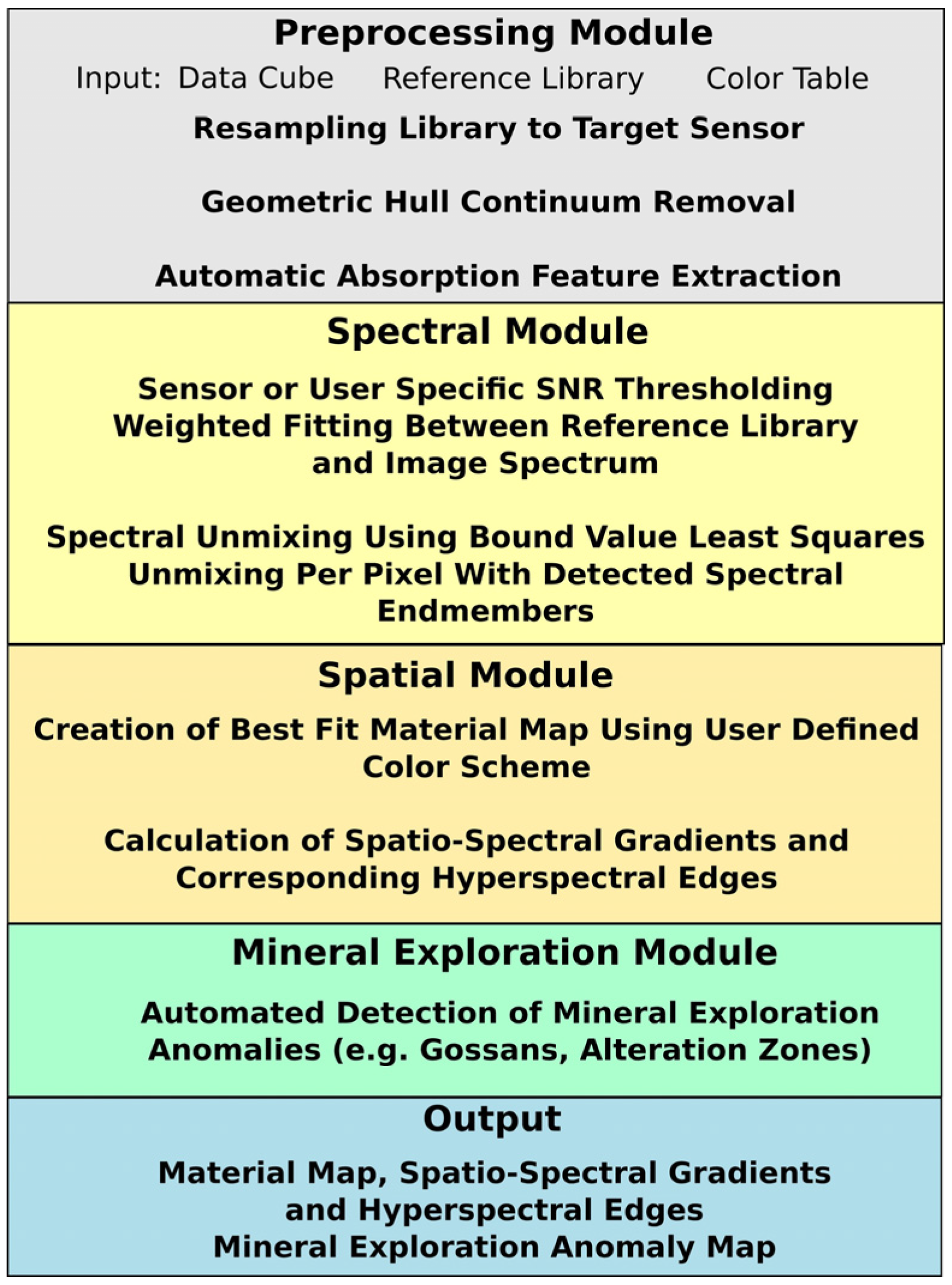
• The fully automated retrieval of characteristic absorption features from reference library spectra and unknown imaging spectroscopy data using the geometric hull approach [14].
• The explicit incorporation of extended sensor parameters (e.g., the sensors Point Spread Function (PSF), spectral Signal to Noise Ratio (SNR) and the related image SNR.
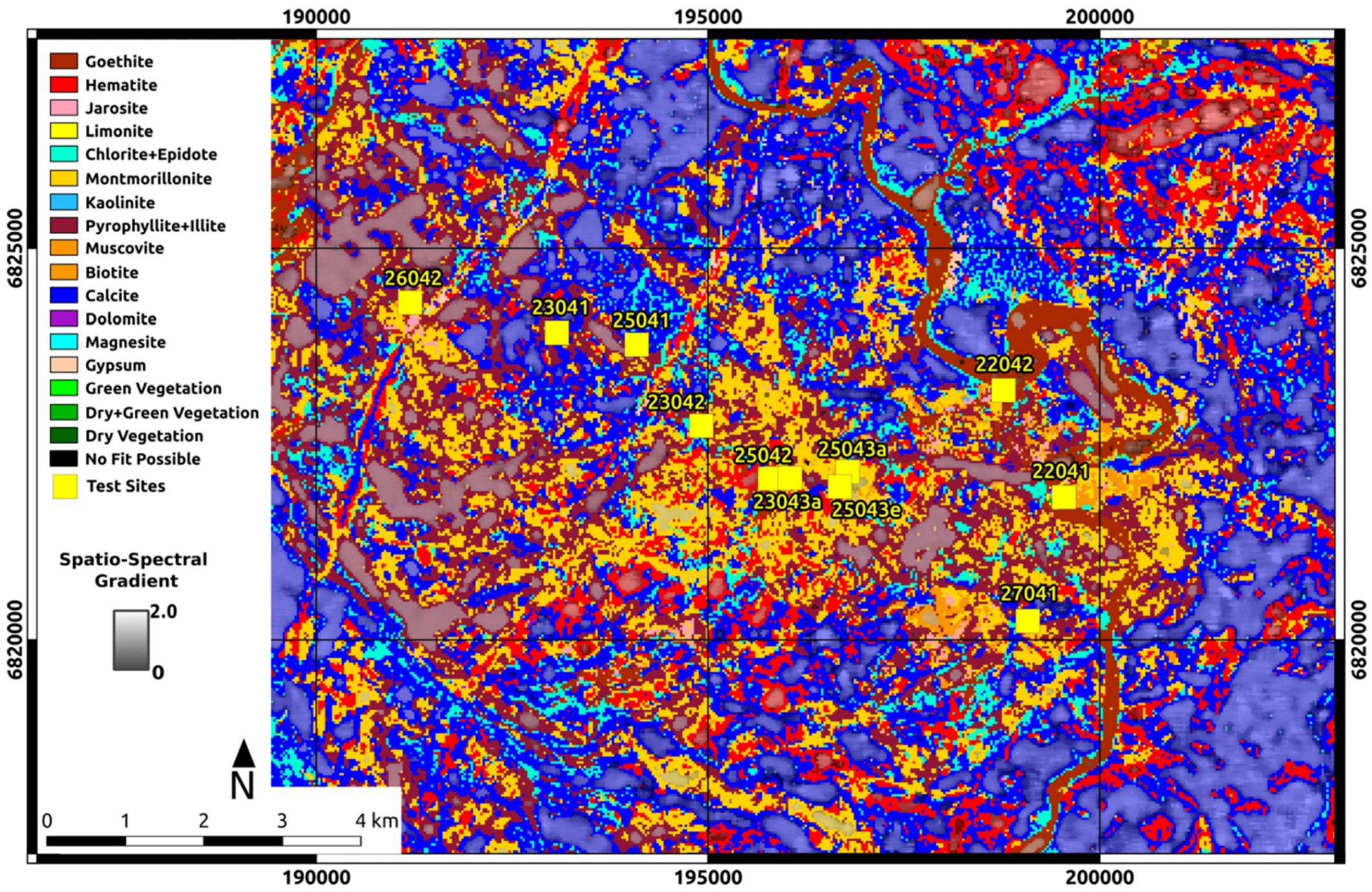
• The calculation of spatio-spectral gradients.
• The automated extraction of mineral anomalies (hydrothermal alteration zones and gossan zones) according to geologic expert knowledge.

Hyperspectral data from HyMAP and simulated EnMAP data [15] is used to test and illustrate the performance of the here proposed EnGeoMAP 2.0 algorithm at the hydrothermal gold-alunite deposit in Rodalquilar Spain [16] and the Haib River porphyry copper deposit in southern Namibia [17]. These results can then be used to assess the performance of the spaceborne EnMAP sensor to characterize the distinct mineral zonation patterns at both test sites. Results from Hyperion data from both test sites are shown as supplementary material considering the well-known problems of this first spaceborne technology demonstrator such as radiometric miscalibration [18] and a low spectral signal to noise ratio [19].

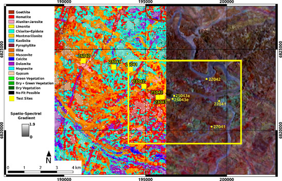
2. Study Sites

The study sites for field verification work were chosen due to their semi-arid (Rodalquilar) and arid (Haib River) climatic conditions that facilitate the usage of hyperspectral spaceborne sensors for surface cover type mapping. Data of both sites were acquired with the hyperspectral airborne sensor HyMAP [2], which also served as input for the simulation of EnMAP data [15]. Hyperion data is additionally available for both test sites. The significantly large lateral extent of the mineralized zone (Haib river) and the large extent of the hydrothermal alteration zones (Rodalquilar) [20] make them unique natural test sites for the mineral mapping performance of spaceborne sensors via automated algorithms.

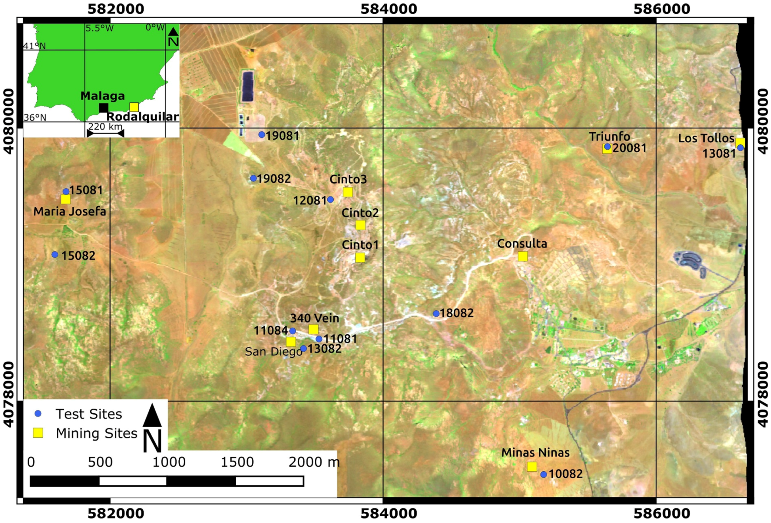
2.1. The Rodalquilar Mineral Deposits

The Rodalquilar caldera is one of three calderas that are situated in the south-eastern part of Spain 24 km east of Almeria. The Rodalquilar, Lomilla and the Los Frailes calderas are part of the Miocene Cabo de Gata volcanic field [21]. The Rodalquilar caldera together with the superimposed Lomilla caldera host the economically relevant gold-silver, lead-zinc-silver-gold and alunite deposits in contrast to the unmineralized Los Frailes caldera [22,23]. The mineral deposit sites near Rodaquilar are shown in Figure 1. Mining operations near Rodalquilar started around 1880 and continued until 1966 with a total amount of 6 t of recovered gold and minor, lead and zinc [21]. Renewed exploration activity for gold commenced during the 1980s together with three years of mining activity [16]. After that the mines closed down in the early 1990s.

The former exploration activity included the appreciation of the large lateral and vertical extent of the hydrothermal alteration zones at the Rodalquilar deposits [22]. These zones consist of an inner silicic alteration zone that grades into an outer advanced argillic alteration zone, which itself is followed by an argillic alteration [16]. The silicic alteration zone is dominated by massive vuggy silica, which documents the extreme acidic conditions during the formation of the mineral deposit sites [21]. This zone is followed by a zone of advanced argillic alteration, which is dominated by quartz and alunite ±pyrophyllite [16]. The advanced argillic zone grades into the argillic alteration zone dominated by quartz, kaolinite and illite and is followed by the propylitic zone, which is dominated by quartz, chlorite, K feldspar, vermiculite, smectite and calcite [16].

Figure 1. HyMAP composite of the main part of the Rodalquilar caldera (R: 2225 nm, G: 911 nm, B: 556 nm), with the locations of the former mining sites in the greater Rodalquilar area. This band combination highlights vegetation in bright green colors.

Figure 1. HyMAP composite of the main part of the Rodalquilar caldera (R: 2225 nm, G: 911 nm, B: 556 nm), with the locations of the former mining sites in the greater Rodalquilar area. This band combination highlights vegetation in bright green colors.

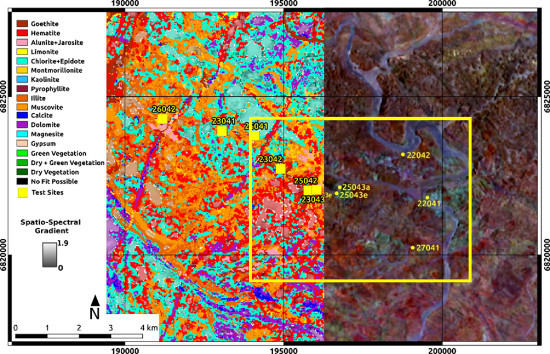
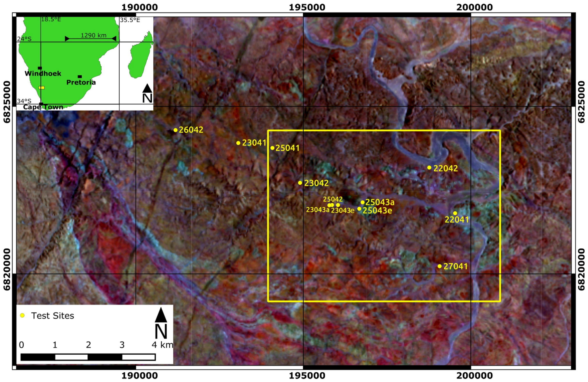
2.2. The Haib River Porphyry Copper-Molybdenum Deposit

The Haib river deposit is one of the oldest known porphyry copper deposits in the world with an age of ~2.0 Ga situated in the Vioolsdrif Intrusive Suite [24]. The mineral deposit site, shown in Figure 2, is located 7 km north of the Orange River 27 km east of Noordoewer. The main mineralization is hosted in the Haib River quartz-felspar porphyry, which is a subsection of the larger Vioolsdrif Intrusive Suite [25]. Mineral exploration activities were initially carried out by Rio Tinto Exploration (Pty) Ltd., in the 1970s [25]. The major copper mineral is chalcopyrite, which is disseminated throughout the Haib porphyry stock with a total volume of less than 0.5% [17]. The Haib river deposit exhibits a well-developed oxidized capping [25], which itself is an attractive exploration target. This capping can be found through multispectral and hyperspectral spaceborne remote sensing techniques [14].

Minnitt [17] initially identified three distinct alteration zone assemblages in the Haib river: the propylitic zone (dominated by chlorite, epidote and carbonate), the phyllic zone (dominated by quartz, sericite and pyrite) and the K-feldspar-biotite zone [17]. The initial Haib porphyry stock was overprinted by a second stage phyllic alteration event, which introduced the metal bearing hydrothermal fluids to the Haib porphyry stock [17]. Work by Barr and Reid [25] verifies the presence of distinct hydrothermal alteration zones showing the presence of a chlorite-sericite dominated zone and a quartz-sericite alteration zone. However, they argue against the classical overprinted porphyry copper model of Minnitt [17], stating that the metal rich fluids interacted with metavolcanic (greenschist-facies) rocks rather than unaltered volcanic rocks during the time of ore formation [25]. The presence of the well-developed oxidized capping together with the hydrothermal alteration zones at a scale of 3 × 11 km facilitates the testing and demonstration of EnGeoMAP 2.0 on spaceborne imaging spectroscopy data.

Figure 2. Simulated EnMAP composite (R: 2226 nm, G: 912 nm, B: 554 nm), of the Haib River deposit in the lower Orange River region. Zone of main mineralization outlined in yellow, field spectroscopy sites displayed as yellow circles. This band combination highlights iron oxide bearing surfaces in red, whilst areas with abundant clay minerals are highlighted in blue-green colors.

Figure 2. Simulated EnMAP composite (R: 2226 nm, G: 912 nm, B: 554 nm), of the Haib River deposit in the lower Orange River region. Zone of main mineralization outlined in yellow, field spectroscopy sites displayed as yellow circles. This band combination highlights iron oxide bearing surfaces in red, whilst areas with abundant clay minerals are highlighted in blue-green colors.

3. Fieldwork and Preprocessing

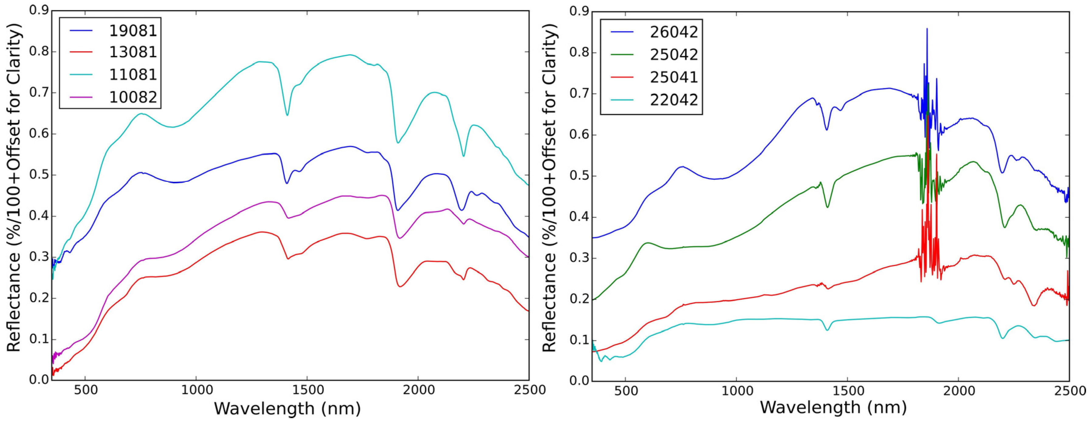
3.1. Fieldwork

Field spectroscopy at the test sites, shown in Figure 1 and Figure 2 was carried out with a portable ASD spectrometer for in situ validation measurements. Each test site was subdivided into a plot of subsets that resembles the spatial coverage of a central pixel together with its immediate neighborhood pixels (3 × 3 pixel). Only those areas were considered as test sites that showed low relief or significant slope on the scale of a 3 × 3 pixel set.

The central pixel was covered with a set of nine evenly spaced subsets of one square meter, whilst the neighborhood pixels were only characterized through one subset at their pixel centers.

This approach also enables Gaussian weighting of the subset field-spectra according to the distance of the subplots to the center of the central pixel. Examples of PSF weighted field spectra are shown in Figure 3. Some spectra were measured with a contact probe, due unfavorable weather conditions. Measurements with a bare fiber setup were carried out during good weather conditions. Surface samples were collected after the field spectroscopy measurements for later laboratory spectroscopic analysis. The spectral sampling could be further improved by a denser set of field spectroscopic samples in the neighboring pixels.

3.2. Data Preprocessing

Airborne hyperspectral data from the HyMap imaging spectrometer [2], was preprocessed using the state of the art Parametric Geocoding approach (PARGE) [26] for geometric correction, and the ATCOR approach [27] for at-ground reflectance retrieval.

The hyperspectral spaceborne data takes of the Hyperion sensor aboard EO-1, which are listed in the reference section have been preprocessed to at-ground reflectance using the Hyperion preprocessing chain [28]. This approach includes the reduction of miscalibration effects noticeable as striping artifacts in the data [18] and an atmospheric correction routine, which has been designed for the EnMAP Toolbox [29], which is based on the theoretical framework of ATCOR [30]. The Hyperion data used in this study is listed in

Table A1. Hyperion data used in this study.

Location	Scene ID
Rodalquilar (Spain)	EO1H1990342003037110PZ
Rodalquilar (Spain)	EO1H1990342003060110KZ
Haib (Namibia)	EO1H1760802013267110KF
Haib (Namibia)	EO1H1760802014013110PF
Haib (Namibia)	EO1H1760802014066110K2
Haib (Namibia)	EO1H1760802014347110KF

of Appendix A. EnMAP data was simulated from the hyperspectral airborne reflectance mosaics of HyMap using the EnMAP End to End simulation tool [15]. The simulation tool involves forward modeling of the reflectance mosaic data to EnMAP at sensor radiance and backward modeling using the EnMAP atmospheric correction module [15]. This elaborate process is carried out to retrieve close to real world simulated EnMAP data from airborne hyperspectral data. This simulated data can now be used to test new applications to the EnMAP mission, such as the here proposed EnGeoMAP 2.0, under the most realistic conditions possible.

Figure 3. PSF weighted field spectra from test sites from the Rodalquilar caldera (left) and the Haib river deposit (right). Contact probe PSF spectra are the smooth spectra.

Figure 3. PSF weighted field spectra from test sites from the Rodalquilar caldera (left) and the Haib river deposit (right). Contact probe PSF spectra are the smooth spectra.

4. The EnGeoMAP 2.0 Process

The EnGeoMAP 2.0 workflow involves four major steps, which are illustrated in Figure 4. The first and most important part is the concept of fully automated absorption feature characterization for the analysis of imaging spectroscopy data using the geometric hull feature extraction [14]. It is part of the EnGeoMAP 2.0 preprocessing module.

Figure 4. Modular processing workflow for mineral and material identification and characterization with EnGeoMAP 2.0.

Figure 4. Modular processing workflow for mineral and material identification and characterization with EnGeoMAP 2.0.

The spectral module involves either a user dependent or sensor dependent spectral SNR weighted fitting of the unknown image spectrum to the mineral reference library. The weighted fitting is performed according to the well-known Tetracorder and MICA processes [9,10]. Only the weighted physics-based absorption features are used for this material characterization process [9,10]. The difference between the Tetracorder and MICA algorithms to the EnGeoMAP 2.0 algorithm is the explicit user determined usage of either sensor dependent SNR thresholds or preset thresholds for significance analysis of the extracted absorption feature information. The final step in the spectral module is the fully constrained linear unmixing of the continuum removed image spectrum, with only those library endmembers, that have been detected in the previous step.

This input is now used in the spatial module for the calculation of spatio-spectral gradients using hyperspectral edge detection [31,32]. This concept has not yet been incorporated into automated expert systems for the analysis of imaging spectroscopy data. The spatial module also supplies a best weighted fit material map based on a user defined color scheme, similar to the maps of the USGS Tetracorder and MICA algorithms [9,10]. The final step is carried out in the mineral exploration module, which exploits the best fit material map information for the automatic delineation of mineral exploration anomalies, such as gossan and alteration zones. Supplement 1 shows the process of feature extraction using the geometric hull in form of pseudocode. The automated extraction of mineral anomalies is shown in Figure S1 as flowchart.

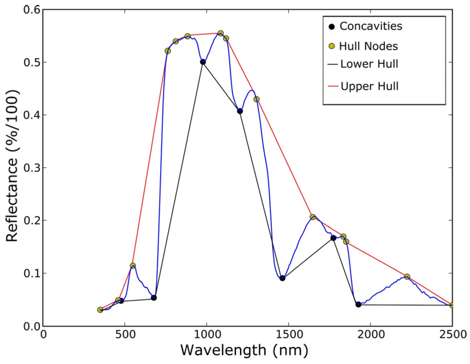
4.1. Automated Identification of Characteristic Absorption Bands

Distinctive absorption features in reflectance spectra have long been used to characterize minerals from reflectance spectroscopic data [33,34]. Material specific absorption bands in the visible and near infrared (VNIR) may represent potential electronic transitions, that could indicate ferrous and ferric iron abundance in the inspected material [34,35]. Vibrational transitions of OH groups in minerals can cause characteristic absorption features in the short wave infrared (SWIR), that may indicate the abundance of clay minerals [34]. The geometric hull technique [14] is used in the here presented version (2.0) of EnGeoMAP. It is able to automatically extract the concave absorption features in the reflectance spectrum without any explicit a priori knowledge of the reflectance spectrum [14]. The geometric hull [14] is determined by firstly detecting the absorption peaks in a reflectance spectrum via division of a smoothed spectrum by its further successively smoothed representation. Linear interpolation between the absorption peaks is carried out to construct a lower hull to the reflectance spectrum as shown in Figure 5. The lower hull is subtracted from the input spectrum resulting in a zero-separated segmentation of the original spectrum. The maximum in each segment is located and serves as node for the linear interpolation of a first preliminary upper hull of the input spectrum. The resultant preliminary hull, shown in Figure 5 is further refined by inserting additional hull nodes in segments of the original spectrum that are above the preliminary hull. The resultant geometric hull can then be used to extract the absorption features from the input spectrum as shown for spectra from the GFZ spectral library [36], shown in Figure S2 of Supplement 2.

Figure 5. Calculation of the geometric hull to the USGS spectral library spectrum “Fir Tree” [12].

Figure 5. Calculation of the geometric hull to the USGS spectral library spectrum “Fir Tree” [12].

An example of the automatic feature definition of spectra from the USGS digital spectral library [12] is shown in Figure 6 in comparison to characteristic absorption features that have been defined by spectroscopic expert assessment. Visual inspection of Figure 6 shows the close resemblance of the automated algorithm to the expert defined features. Additional tests with spectra from the USGS digital spectral library [12] and the Tetracorder [9] and MICA [10] expert feature definitions showed that the automated geometric hull feature definition is closest to the expert based feature definition, if compared to the state of the art techniques such as alpha shapes and convex hull [14].

Figure 6. Characteristic absorption features of minerals in the solar reflective region extracted manually by expert knowledge based feature definition (left) and by the fully automated geometric hull technique (middle). Spectral entries belong to the USGS spectral library [12]. The residuals between the geometric hull feature definition and the expert definition are shown in the right image.

Figure 6. Characteristic absorption features of minerals in the solar reflective region extracted manually by expert knowledge based feature definition (left) and by the fully automated geometric hull technique (middle). Spectral entries belong to the USGS spectral library [12]. The residuals between the geometric hull feature definition and the expert definition are shown in the right image.

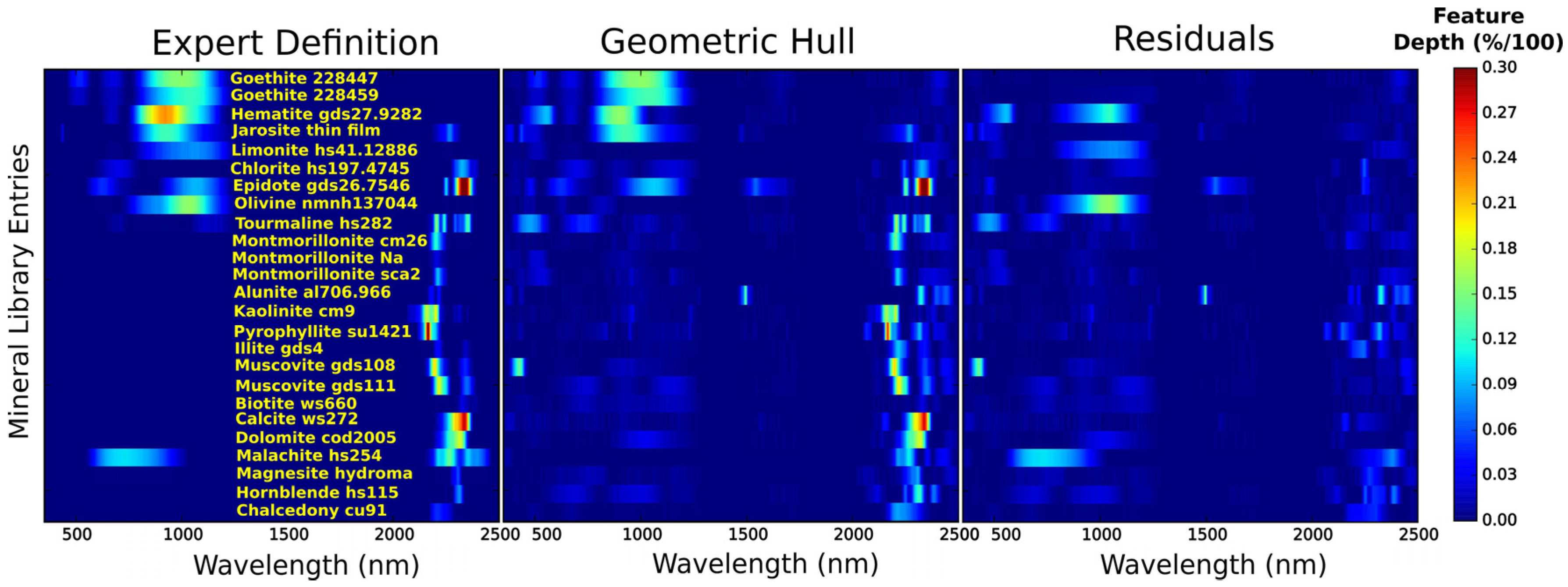
4.2. Continuum Removal for Absorption Band Retrieval

The geometric hull is calculated to the library reference spectra and the unknown pixel spectrum. The geometric hull can now be removed from the corresponding spectrum by dividing the spectrum by its geometric hull (relative continuum removal), or by subtracting the geometric hull from the spectrum (absolute continuum removal). Identified absorption features that are covering a part of the large atmospheric water vapor absorption features at 1900 nm or 1400 nm are excluded from the further analysis process. In the second step the absolute feature depths can now be screened using either user defined minimum absorption depth thresholds for features in the VNIR (up to 1000 nm) and for absorption features in the SWIR (from 1000 to 2500 nm). Features that fall below these two user defined thresholds are also excluded from further analysis.

4.3. User Independent SNR Thresholding

The sensor specific SNR curve can be used for a user input independent evaluation of the absorption depths in the specific channels of an image pixel or a reference library entry.

This has been implemented for those sensors where more detailed SNR information was either published (Hyperion [19] and HyMAP [2]) or otherwise known (EnMAP [15]). The SNR information is now weighted with the image SNR, which was retrieved by dividing the image mean by the image standard deviation in each channel [37]. Now the reflectance of the continuum above each characteristic absorption feature of a spectrum may be used together with the aforementioned SNR information in the respective channel to retrieve the SNR information that is used for a SNR thresholding in each spectral channel. For example, if the SNR value for Hyperion [19] is 40/1 for an albedo level of 30% at 2125 nm and the according calculated absolute absorption depth information at 2125 nm is below this value of 2.5%, then the information in this channel is flagged unreliable and it is excluded from the following analysis steps. Further uncertainties, for example introduced by the atmospheric correction, have not been taken into account.

4.4. Weighted Fitting

The continuum removed data that has passed the aforementioned thresholding step is now weighted using the feature area and the maximum feature depth as thresholds similar to the USGS Tetracorder [9] and MICA [10] algorithms. The fit between the weighted continuum removed image spectrum and the according reference spectra can be calculated by a variety of similarity measures, such as linear regression (as in case of the Tetracorder [9]), or via the Modified Spectral Angle Mapper (MSAM) [38], or by the Spectral Information Divergence (SID) and combinations of the SID with the sine or tangent of the spectral angle [39].

The performance of these similarity measures was tested on a 100 × 100 pixel subset of simulated EnMAP data from the central mining region of Rodalquilar. The results are shown in color coded form in Figure 7 and in Table 1 where the runtime of EnGeoMAP 2.0 is listed for this subset on a single core of an Intel Core i7-4710MQ CPU with 2.5 GHz. A user defined threshold of 2% minimum absorption depth in the VNIR and 3% in the SWIR was used in this comparison. The comparison parameters in Table 1 are runtime, Mean Structural Similarity Index Measure (MSSIM) [40] of the best weighted fit results to the linear regression result, code complexity and overall performance. Table 1 shows that the overall performance is best with the linear correlation. This algorithm has the lowest code complexity and is the fastest of all algorithms. Additionally, no deviation in the best weighted fit material mapping results to the linear regression algorithm can be found because the MSSIM is 1.0. Therefore, the linear correlation (see Equation (1)) is used in EnGeoMAP 2.0 to carry out the fitting that is equal to Tetracorder and MICA [9,10]. With X_i being the continuum removed weighted absorption depth of the unknown image spectrum in spectral channel i with $\overline{\text{X}}$ being the mean of the weighted absorption depth vector X. Y_i being the continuum removed weighted absorption depth of a single reference spectrum in spectral channel i with $\overline{\text{Y}}$ being the mean of the weighted absorption depth vector Y. C is the linear correlation coefficient between the two weighted absorption depth vectors indicating the similarity of the unknown spectrum to the reference spectrum. Correlation results calculated for data from the Rodalquilar deposit area are shown in Supplement 3. Results for the Haib river deposit are shown in Supplement 4.

$$\mathrm{C}=\frac{{{\displaystyle \sum }}_{\mathrm{i}=1}^{\mathrm{n}}\left({\mathrm{X}}_{\mathrm{i}}-\overline{\text{X}})({\mathrm{Y}}_{\mathrm{i}}-\overline{\text{Y}}\right)}{\sqrt{{{\displaystyle \sum }}_{\mathrm{i}=1}^{\mathrm{n}}{({\mathrm{X}}_{\mathrm{i}}-\overline{\text{X}})}^2}\sqrt{{{\displaystyle \sum }}_{\mathrm{i}=1}^{\mathrm{n}}{({\mathrm{Y}}_{\mathrm{i}}-\overline{\text{Y}})}^2}}$$

(1)

Now the best weighted fit value can be retrieved for each pixel, which identifies the best weighted fit mineral or material. The resultant best fit material maps are shown in Figure 7. A detailed survey on spectral similarity measures can be found in van der Meer 2006 [41].

Figure 7. Color coded best weighted fit results from EnGeoMAP 2.0 for the simulated EnMAP Rodalquilar subset (A) Color composite (R: 2226 nm, G: 912 nm, B: 554 nm) using different fitting methods; (B) Linear Regression; (C) Linear Correlation; (D) Modified Spectral Angle Mapper (MSAM); (E) Spectral Information Divergence (SID); (F) SID × sin(MSAM); (G) SID × tan(MSAM). Please note that there are only small differences in the extent of the classified kaolinite area in the upper center between (B); (C); (D) and (E); (F); (G).

Figure 7. Color coded best weighted fit results from EnGeoMAP 2.0 for the simulated EnMAP Rodalquilar subset (A) Color composite (R: 2226 nm, G: 912 nm, B: 554 nm) using different fitting methods; (B) Linear Regression; (C) Linear Correlation; (D) Modified Spectral Angle Mapper (MSAM); (E) Spectral Information Divergence (SID); (F) SID × sin(MSAM); (G) SID × tan(MSAM). Please note that there are only small differences in the extent of the classified kaolinite area in the upper center between (B); (C); (D) and (E); (F); (G).

Table 1. Performance evaluation of state of the art spectral similarity measures using a 100 × 100 pixel simulated EnMAP subset from Rodalquilar in an EnGeoMAP 2.0 analysis.

Method	Runtime (s)	MSSIM with Linear Regression	Algorithm Complexity	Overall Performance
Linear Correlation	61.44	1.0	1	A
Linear Regression	92.38	1.0	2	B
MSAM	130.04	1.0	2	C
SID	131.67	0.889	2	D
SIDx(SIN(MSAM))	206.29	0.89	3	E
SIDx(TAN(MSAM))	300.77	0.89	3	F

Table 1. Performance evaluation of state of the art spectral similarity measures using a 100 × 100 pixel simulated EnMAP subset from Rodalquilar in an EnGeoMAP 2.0 analysis.

Method	Runtime (s)	MSSIM with Linear Regression	Algorithm Complexity	Overall Performance
Linear Correlation	61.44	1.0	1	A
Linear Regression	92.38	1.0	2	B
MSAM	130.04	1.0	2	C
SID	131.67	0.889	2	D
SIDx(SIN(MSAM))	206.29	0.89	3	E
SIDx(TAN(MSAM))	300.77	0.89	3	F

As a final step the absolute absorption depth information of each image pixel may now be analyzed using fully constrained linear unmixing with the absolute absorption depths of only those mineral and material endmembers that have been detected by the weighted fitting in the previous analysis step. Fully constrained linear unmixing was used as it represents the most widely used unmixing technique today [42]. This unmixing information is now used to reconstruct the absolute absorption depths at an image pixel via its detected reference spectra endmembers.

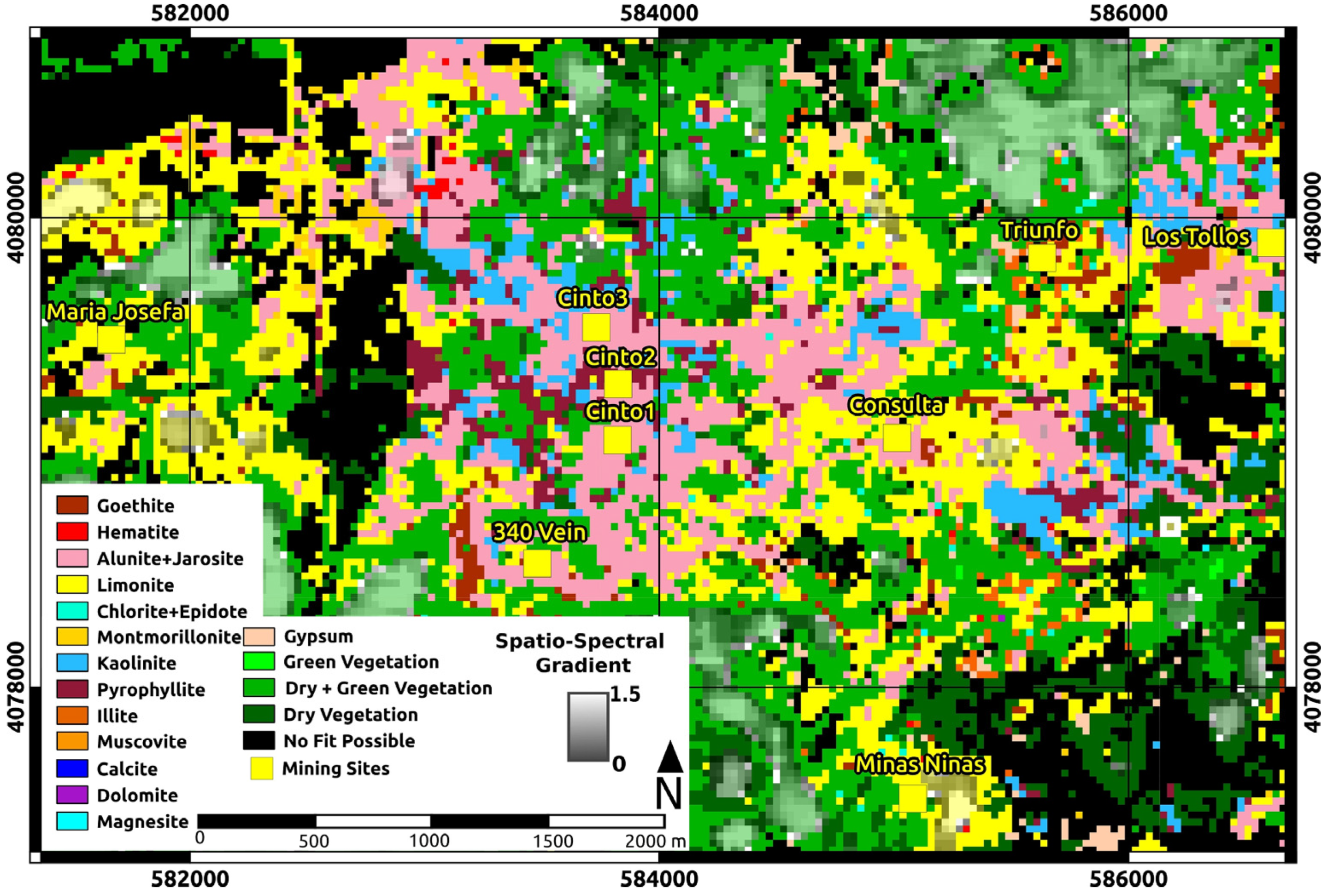
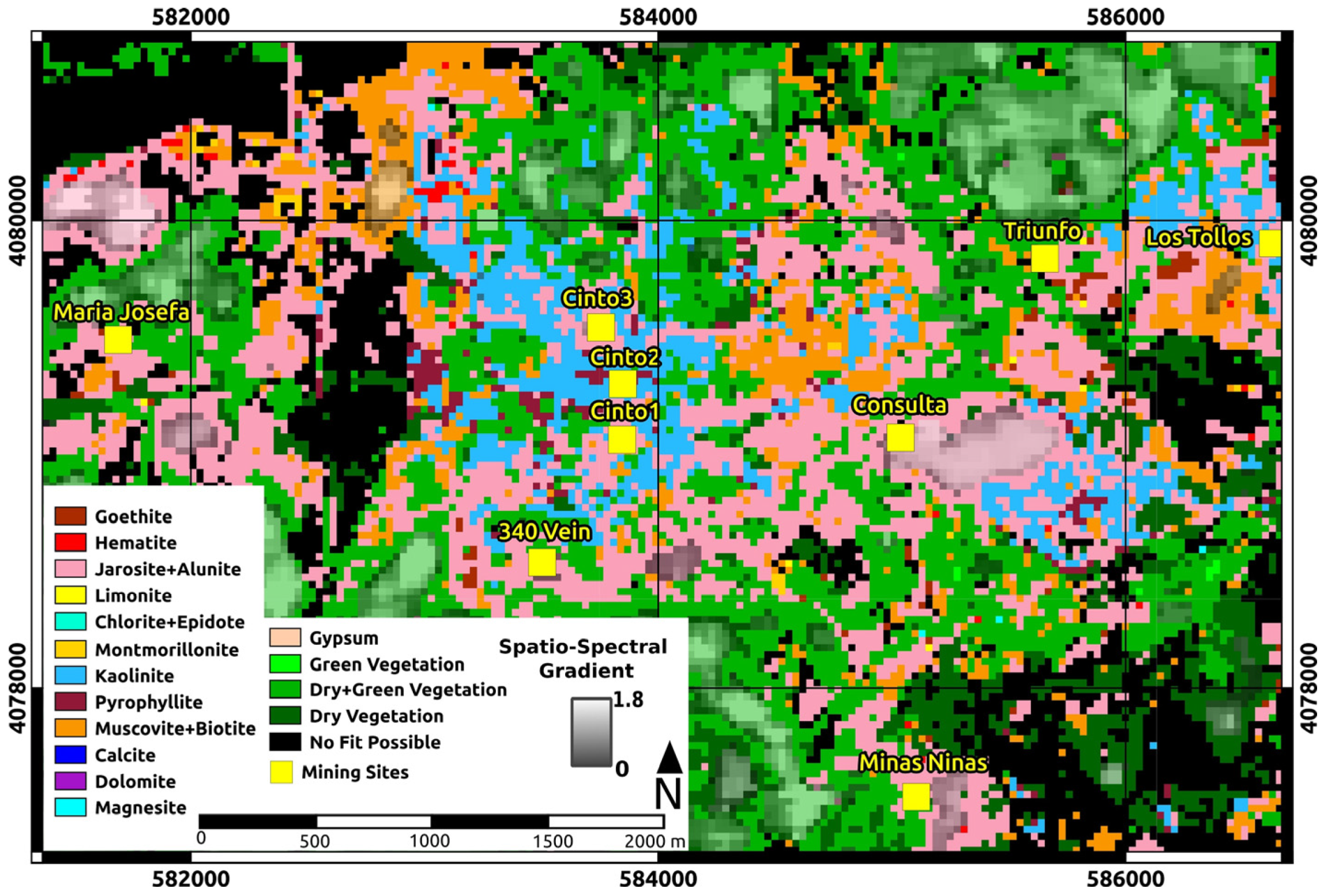
4.5. Calculation of Spatio-Spectral Gradients

The unmixed image data is now analyzed for spatio-spectral gradients using the Busyness Multiple Correlation Edge Detector (BMCED) approach [31,32] for the localization of spatio-spectral gradients. The gradient detection proposed here is carried out by a moving window based operator that moves across all lines (l) and samples (s) of the data cube calculating the linear correlation (see Equation (1)) (LCorr) of the neighborhood pixels with the central pixel at position (i,j), shown in Equation (2). The gradient (Grad) is detected by weighting the linear correlation result with a kernel of coefficients calculated by a Laplacian of Gaussian function (see Equation (3)) with × and y being the coordinates of the pixels inside the moving window. Sigma is the standard deviation of the Gaussian function used.

$${\text{Grad}}_{\mathrm{i},\mathrm{j}=0}^{\mathrm{i},\mathrm{j}=\mathrm{s},\mathrm{l}}={\text{LoG}}_{\mathrm{i},\mathrm{j}}\left({\text{LCorr}}_{\mathrm{i},\mathrm{j}}\right)$$

(2)

$$\text{LoG}=-\frac{1}{\mathsf{\pi }{\mathsf{\sigma }}^4}{\mathrm{e}}^{-\frac{{\mathrm{x}}^2+{\mathrm{y}}^2}{2{\mathsf{\sigma }}^2}}(1-\frac{{\mathrm{x}}^2+{\mathrm{y}}^2}{2{\mathsf{\sigma }}^2})$$

(3)

$${\mathsf{\sigma }}_{\text{sensor}}=\frac{{\text{FWHM}}_{\text{sensor}}}{2\sqrt{2\text{ln}2}}$$

(4)

The standard deviation in Equation (3) can be adjusted towards a specific sensor PSF using a sensor dependent standard deviation, which can be calculated through Equation (4). With σ_sensor being the sensor adopted standard deviation to be used in Equation (3) and FWHM_sensor being the sensors spatial full width at half maximum. The resulting gradient map can now be filtered with a modified Canny edge filter [43] where the initial Sobel operator has been replaced by the Prewitt operator for hyperspectral edge detection [32].

4.6. Automated Retrieval of Potential Exploration Anomalies

The main aim of imaging spectroscopy in mineral exploration is the identification of minerals and their specific spatial distribution pattern to identify zones of high ore potential. These zones of highest prospectivity may then aid more detailed exploration work in the field. The critical factor for the success of such an operation is to link the geological expert knowledge, e.g., from exploration models, to the results derived from imaging spectroscopy in order to identify exploration targets of interest over large areas [44,45]. This can be achieved using the best weighted fit material maps.

Gossan zones may show a characteristic oxidation pattern of metal sulfide minerals, which may indicate the abundance of copper bearing sulfide minerals (e.g., chalcopyrite) rather than the abundance of purely iron bearing sulfides (e.g., jarosite) [46]. An iron alteration zone pattern can be created from this geologic expert knowledge where hematite outlines the zone most proximal to the chalcopyrite mineralization. Goethite surrounds these hematite zones where the content of pyrite exceeds those of chalcopyrite grading outwards into the most distal zone with a dominance of jarosite, which mainly indicates the oxidation of pyrite [47]. This subdivision of gossan areas into three zones can now be exploited for an automatic detection of gossan mineral anomalies, which is described below. At first all inner zones, which are represented by pixels with a best weighted fit value with hematite are extracted. This is also carried out with the middle zone represented by goethite pixels and the distal zone represented by jarosite pixels. Now the three zones are transformed to binary images. Each zone of continuous hematite pixels is now grown via iterative binary morphological dilation [48] until at least one zone of goethite and jarosite are intersected by the dilated innermost zone. This process is repeated until all adjacent goethite and jarosite zones are found for each continuous hematite zone. The workflow is shown in Figure S1 of Supplement 1.

5. Results of EnGeoMAP 2.0

Results from EnGeoMAP 2.0 were calculated from HyMAP and simulated EnMAP data over the Rodalquilar gold-alunite deposit in Spain and the Haib River porphyry copper-molybdenum deposit. EnGeoMAP 2.0 results from the airborne HyMAP sensor serve as benchmark for the results calculated from the hyperspectral spaceborne sensors. The GFZ spectral reference library [36], shown in Figure S2 was used to create the here presented EnGeoMAP 2.0 results. Vegetation spectra from the USGS digital spectral library [12] were additionally included: the spectra “fir tree” and “green grass” represent green vegetation, the spectrum “dry and green grass” was used as representative for dry and green vegetation and the spectrum “dry long grass” was used as reference spectrum for dry vegetation. Additional results from the USGS digital spectral library [12] and endmember mixtures thereof are also shown. EnGeoMAP 2.0 results from Hyperion data are separately shown in Supplement 5 to preserve the compactness of the article.

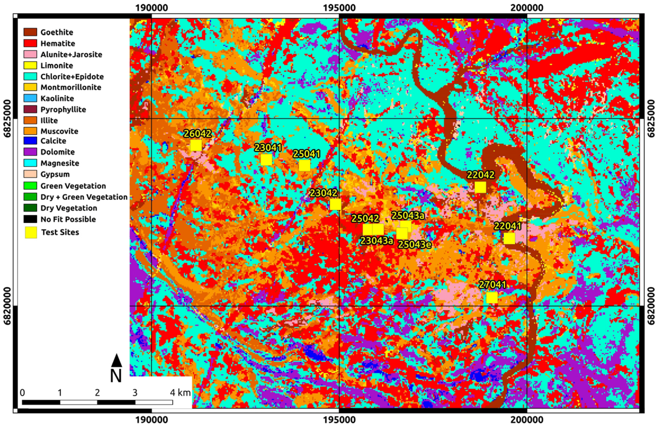
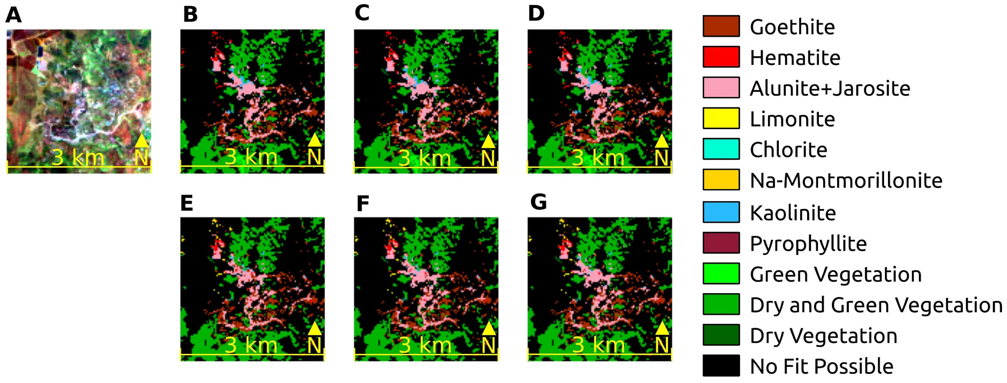
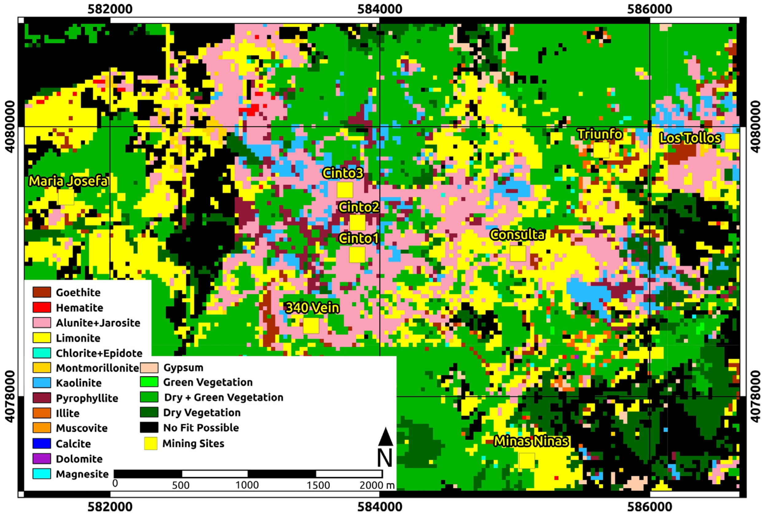
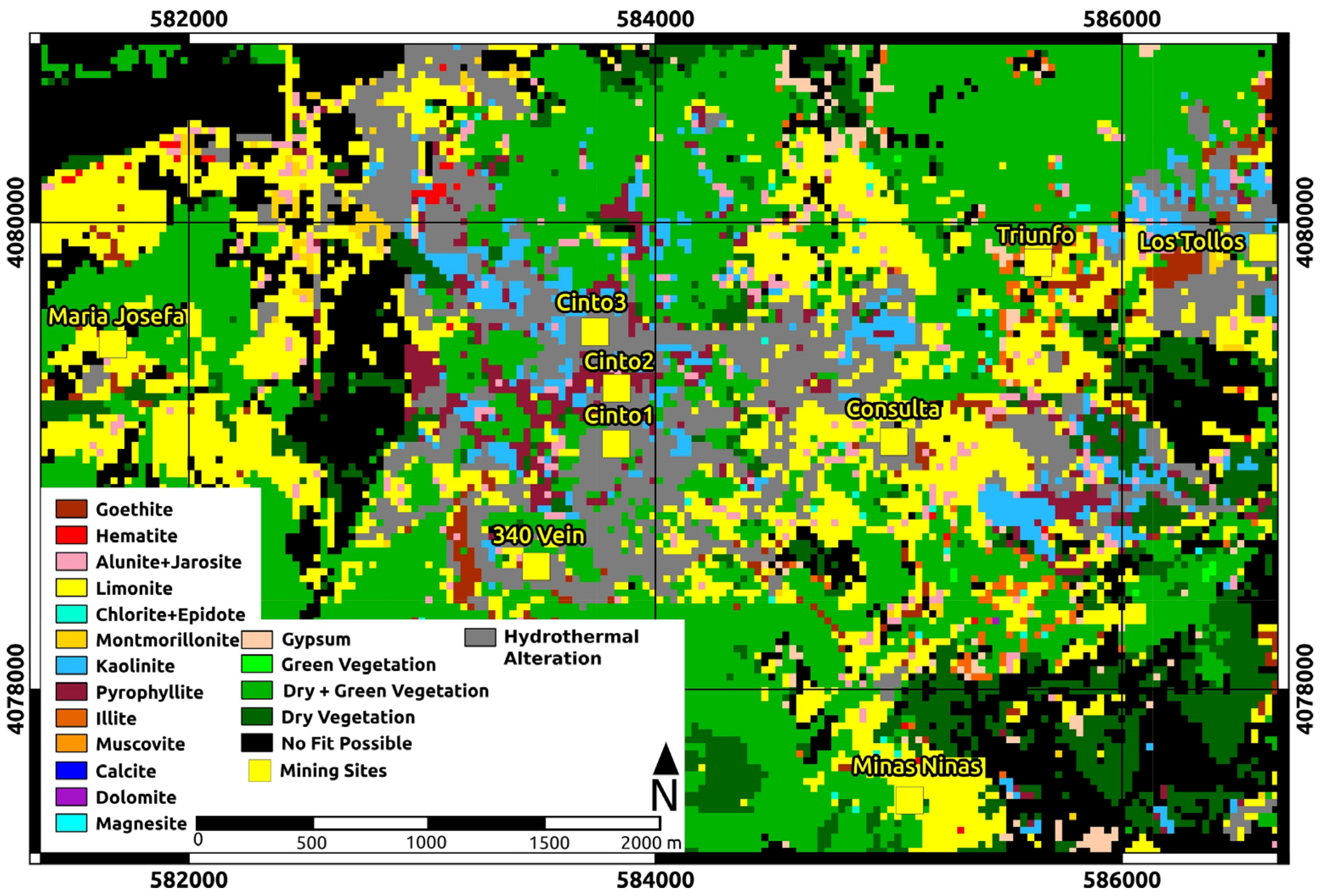
5.1. Results from the Rodalquilar Deposits Using the GFZ Spectral Library

A material map calculated from simulated EnMAP data is shown in Figure 8. The two major alteration centers that have been described in literature [16,21] can be easily identified here, with the main alteration center in the central part of Figure 8. This has been the center of the gold mining operations near Rodalquilar. The second prominent alteration center to the east of the image is situated around the Los Tollos deposit, where alunite was mined [21]. Large areas of rock dumps are situated to the east of the Consulta mine and to the northwest of the Cinto deposits, as also shown in Figure 1. These two sites contain rock waste material, which is dominated by alunite, jarosite and kaolinite. The same alteration centers above have also been noticed and described in previous multispectral investigations [21] and furthermore in hyperspectral studies [20,49].

Figure 9 shows the spatio-spectral gradient as overlay to the material analysis results. The strongest gradients can be found in the vegetation around the alteration centers and to the north and south of Maria Josefa. These gradients can be explained by the spatial mixture of vegetation cover with iron oxide bearing soil, as shown in Figure 10. Here we see that the vegetation patches in the 30 m pixel of EnMAP also contain areas dominated by iron oxide, mapped as hematite shown in the 5 m pixel of the HyMAP results in Figure 10. This complex spatial mixture of iron bearing soils and vegetation, which affects the iron absorption feature at 900 nm has also been reported by Richter (2010) [50]. The main difference between the material analysis maps from the simulated EnMAP data to the HyMAP data is the change from hematite to limonite in the analysis results. This can be attributed to complex spectral mixtures in the 30 m EnMAP pixels. Nevertheless, limonite (FeOOH*n(H₂O)) shows a partial spectral overlap between its absorption features and the absorption features of other iron bearing minerals, such as goethite and hematite. This can cause the classification of the iron bearing soils in large EnMAP pixels as limonite due to a sub pixel mixture of small proportions of vegetation and iron bearing soils [50]. Additionally, a high quality data input is necessary for the EnGeoMAP process, which needs to completely remove the atmospheric gas and water vapor absorption bands, especially in the VNIR up until 1200 nm to ensure the correct classification of iron bearing minerals.

Figure 8. EnGeoMAP 2.0 best fit material map calculated from simulated EnMAP data, using sensor dependent absorption depth thresholding. Note the main advanced argillic alteration characterized by alunite and jarosite in the image center. Please also note the large abundance of alunite and jarosite to the east at Los Tollos.

Figure 8. EnGeoMAP 2.0 best fit material map calculated from simulated EnMAP data, using sensor dependent absorption depth thresholding. Note the main advanced argillic alteration characterized by alunite and jarosite in the image center. Please also note the large abundance of alunite and jarosite to the east at Los Tollos.

Figure 9. EnGeoMAP 2.0 best fit material map, using sensor dependent absorption depth thresholding, with a semi-transparent overlay of the spatio-spectral gradient and prominent gradient edge pixel (non-transparent rim pixel around the gradient patches).

Figure 9. EnGeoMAP 2.0 best fit material map, using sensor dependent absorption depth thresholding, with a semi-transparent overlay of the spatio-spectral gradient and prominent gradient edge pixel (non-transparent rim pixel around the gradient patches).

Figure 10. Best weighted fit material map of EnGeoMAP 2.0 calculated from airborne HyMAP data, which was used as simulation input to produce the EnMAP data.

Figure 10. Best weighted fit material map of EnGeoMAP 2.0 calculated from airborne HyMAP data, which was used as simulation input to produce the EnMAP data.

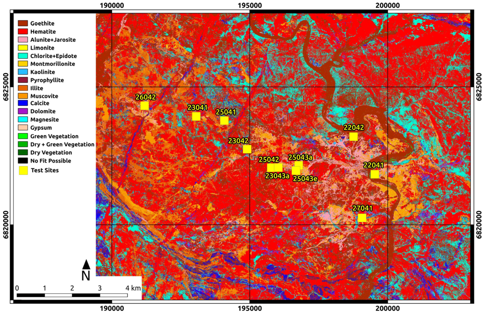
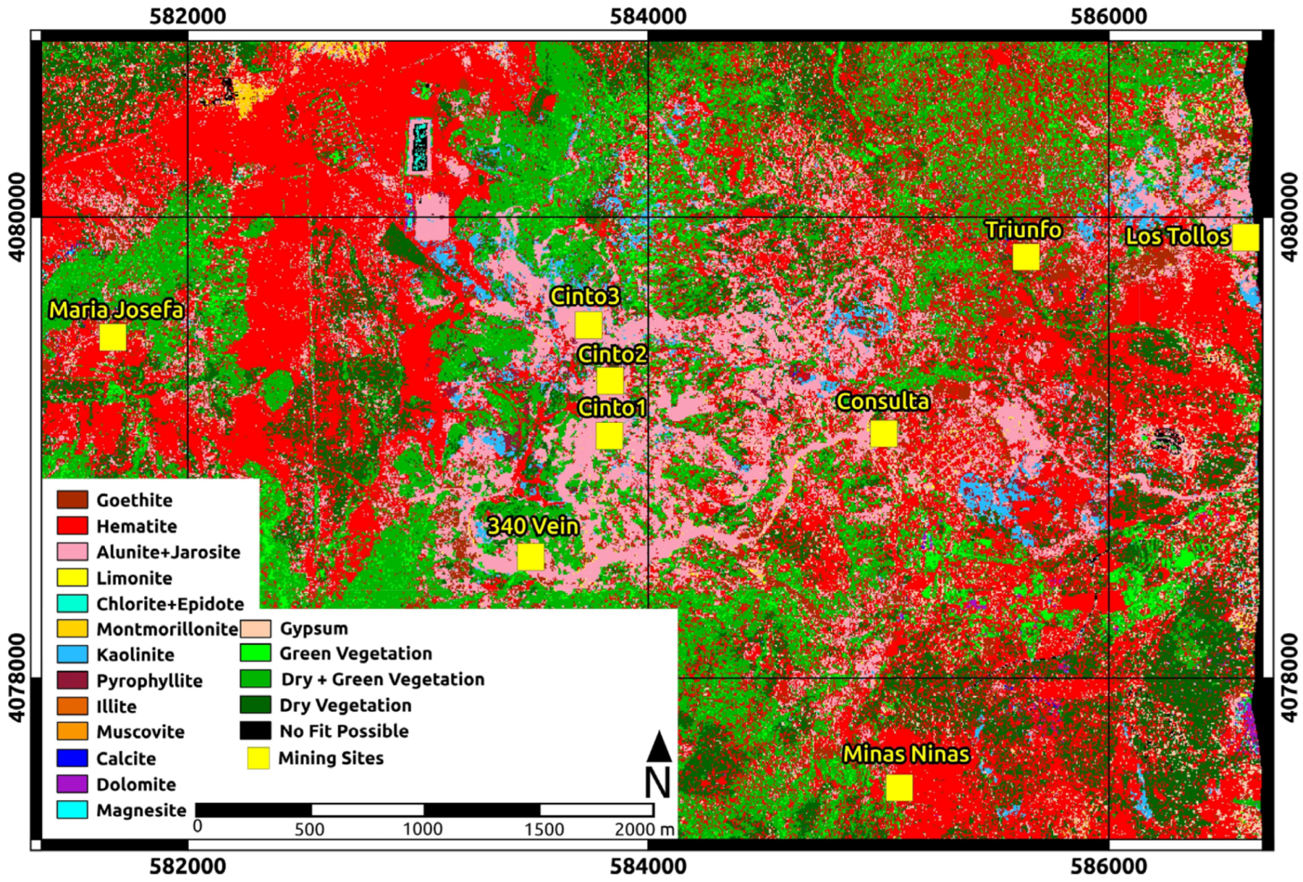
5.2. Results from the Rodalquilar Deposits Using the USGS Digital Spectral Library

A second and third EnGeoMAP 2.0 run was carried out using reference spectra from the USGS digital spectral library, shown in Figure 6. The results are shown in Figure 11 and Figure 12. Figure 11 shows a comparable distribution of pyrophyllite, alunite and kaolinite in the area of the three main deposit sites. However, there is a notable difference as now the iron bearing soils, around the mineral deposit areas are mapped as jarosite instead of as limonite, as shown in Figure 8 and Figure 9. Here the change in the reference spectra causes a dominance of jarosite over hematite. Nevertheless, we are able to see that there is a complex sub EnMAP pixel mixture, between hematite and jarosite, shown in Figure 10. Figure 12 shows an EnGeoMAP 2.0 result that uses simple linear combinations of USGS digital spectral library spectra for the material mapping at the Rodalquilar deposits, which have been described by Bedini et al. [49]. Here we see that the otherwise monotonously mapped zone of kaolinite, alunite and jarosite are dominated by complex mixtures of the minerals kaolinite, alunite, pyrophyllite and illite, as described in Bedini et al. [49]. These different results show that the EnGeoMAP 2.0 results are affected by the entries of the mineral reference library. However, the large zones, associated with vegetation, iron bearing minerals, kaolinite, pyrophyllite and jarosite and alunite have been found throughout the EnGeoMAP 2.0 results. A more detailed geological result can be achieved if users include mineral endmember mixtures to the reference library as shown in Figure 12.

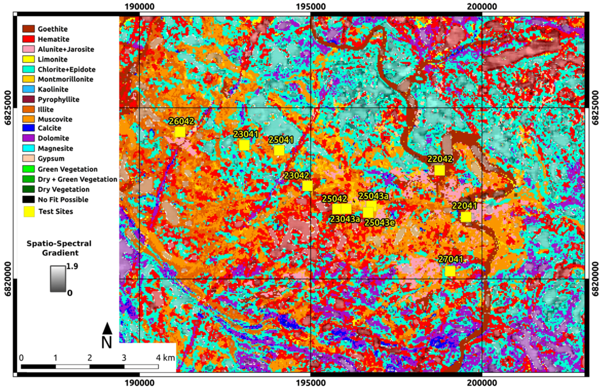
5.3. Results from the Haib River Deposit Using the GFZ Spectral Library

Figure 13 and Figure 14 show mineral maps from the Haib River copper deposit. The Haib River is outlined as goethite bearing. A prominent zone of epidote and chlorite surrounds the center of the main mineralization, which is outlined in Figure 2. These are the parts of the Haib River volcanic rocks that have been subjected to greenschist facies metamorphic conditions [25]. The innermost zone of the mineral deposit stretching from 23042 towards 22042 and 27041 is dominated by characteristic gossan surfaces, showing hematite, goethite and jarosite. The main entrance to an area where test mining was carried out can be found between 25042 and 23043a. Here fieldwork showed several tens to hundreds of square-meters covered with malachite staining and gossan. An outer gossan zone can be found at 26042. These innermost and outermost zones can also be found with complex ratio techniques from multispectral sensors such as Landsat-8’s Operational Land Imager [51], EO-1 ALI [1] and Sentinel-2 [52] as shown by earlier studies [53]. A close similarity can be observed if the result from EnMAP data in Figure 13 is visually compared to an analysis of the original HyMAP data in Figure 15. The Haib River is dominated by goethite in both EnGeoMAP 2.0 analysis. Additionally, the epidote and chlorite zone surrounding the main mineralization can be found in both images. Only the small patches of e.g., vegetation in the dry bed of the Haib River cannot be resolved by the EnMAP data. Areas with a strong spatio-spectral gradient in the Figure 14 are attributed to a complex material mix at the sub-EnMAP pixel scale. This is illustrated by the material map calculated from the HyMAP data in Figure 15.

Figure 11. EnGeoMAP 2.0 best fit material map, using sensor dependent absorption depth thresholding, with a semi-transparent overlay of the spatio-spectral gradient using the entries of the USGS digital spectral library [12] as reference spectra.

Figure 11. EnGeoMAP 2.0 best fit material map, using sensor dependent absorption depth thresholding, with a semi-transparent overlay of the spatio-spectral gradient using the entries of the USGS digital spectral library [12] as reference spectra.

Figure 12. EnGeoMAP 2.0 best fit material map, using sensor dependent absorption depth thresholding, with a semi-transparent overlay of the spatio-spectral gradient using the entries of the USGS digital spectral library [12]. Linear combinations of their entries labeled with as “Mix” follow the suggested endmember combinations of Bedini et al., 2009 [49].

Figure 12. EnGeoMAP 2.0 best fit material map, using sensor dependent absorption depth thresholding, with a semi-transparent overlay of the spatio-spectral gradient using the entries of the USGS digital spectral library [12]. Linear combinations of their entries labeled with as “Mix” follow the suggested endmember combinations of Bedini et al., 2009 [49].

Figure 13. EnGeoMAP 2.0 best fit material map calculated from simulated EnMAP data, using sensor dependent absorption depth thresholding. Note the central zone of main mineralization, which is dominated by hematite, goethite and jarosite, surrounded by patches of epidote and chlorite.

Figure 13. EnGeoMAP 2.0 best fit material map calculated from simulated EnMAP data, using sensor dependent absorption depth thresholding. Note the central zone of main mineralization, which is dominated by hematite, goethite and jarosite, surrounded by patches of epidote and chlorite.

Figure 14. EnGeoMAP 2.0 best fit material map calculated from simulated EnMAP data, using sensor dependent absorption depth thresholding. The semi-transparent overlay shows the spatio-spectral gradient. Prominent gradient edge pixel shown as non-transparent rim pixel around the semi-transparent gradient patches.

Figure 14. EnGeoMAP 2.0 best fit material map calculated from simulated EnMAP data, using sensor dependent absorption depth thresholding. The semi-transparent overlay shows the spatio-spectral gradient. Prominent gradient edge pixel shown as non-transparent rim pixel around the semi-transparent gradient patches.

Figure 15. Best weighted fit material map of EnGeoMAP 2.0 calculated from airborne HyMAP data, which was used as simulation input to produce the EnMAP data.

Figure 15. Best weighted fit material map of EnGeoMAP 2.0 calculated from airborne HyMAP data, which was used as simulation input to produce the EnMAP data.

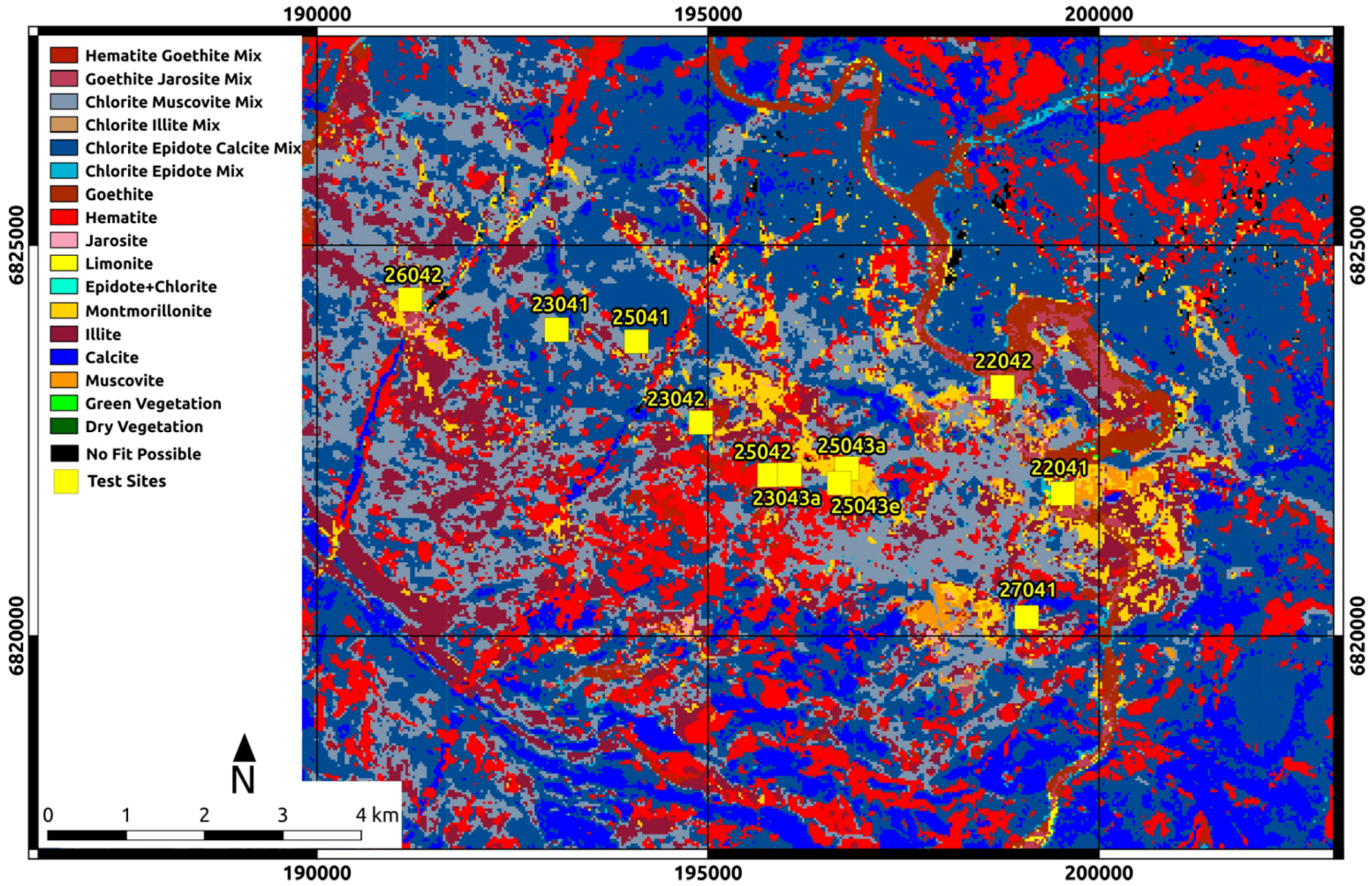
5.4. Results from the Haib River Deposit Using the USGS Digital Spectral Library

Figure 16 shows an EnGeoMAP 2.0 result calculated from simulated EnMAP data from the Haib river complex. The central part of the mineral deposit site and the outermost gossan zone at 26042 are dominated by iron bearing minerals that indicate the presence of gossan surfaces, similar to the results of Figure 13 and Figure 14. The most notable difference between Figure 16 and Figure 13 and Figure 14 is the large presence of calcite instead of epidote or chlorite. Only small spots of epidote and chlorite can be located within the blue patches of calcite in Figure 16. This is an apparent problem of results from expert systems, which has been described by Dalton et al. [54]. They used synthetic mixtures of epidote, chlorite and calcite to improve mineral mapping results of the USGS Tetracorder [54]. A similar approach was also used to produce the EnGeoMAP 2.0 result of Figure 17. The results were produced by using linear combinations of reference spectra from the USGS spectral library [12] according to the mineralogy described by Minnit [17] and Barr and Reid [25]. This leads to a reduction of the calcite dominated areas in favor of a chlorite, epidote, calcite mix together with an epidote and chlorite mix as described in Minnit [17] and Barr and Reid [25]. The proposed approach of Dalton et al. [54] leads to a spatially and geologically more refined image of the Haib river deposit site.

5.5. Automated Delineation of Exploration Anomalies

5.5.1. Rodalquilar

Rodalquilar has been described as an acid-sulfatesulfate gold mineralization [16,55]. The most important alteration zones that are characteristic for the epithermal activity that has been associated with the mineral deposition are the argillic and the advanced argillic alteration zones [22]. Here the minerals alunite and jarosite will be used as proxies for the advanced argillic alteration zone, which is proximal to the ore zone [22]. Kaolinite and illite will serve as proxies for the argillic alteration zone [22]. Figure 18 shows the identified acid-sulfatesulfate mineral exploration anomalies in grey resembling the advanced argillic alteration, calculated from simulated EnMAP data. It is overlain over the best fit mineral map also derived from EnMAP data. The grey areas outline the main mineral deposit zone around the Cinto deposits. The alteration center around Los Tollos is also clearly visible together with the mine dump material directly to the east of Consulta.

Figure 16. EnGeoMAP 2.0 best fit material map, using sensor dependent absorption depth thresholding, with a semi-transparent overlay of the spatio-spectral gradient using the entries of the USGS digital spectral library [12] as reference spectra.

Figure 16. EnGeoMAP 2.0 best fit material map, using sensor dependent absorption depth thresholding, with a semi-transparent overlay of the spatio-spectral gradient using the entries of the USGS digital spectral library [12] as reference spectra.

Figure 17. EnGeoMAP 2.0 best fit material map, using sensor dependent absorption depth thresholding, using the entries of the USGS digital spectral library [12]. Linear combinations of their entries labeled with as “Mix” follow the endmember combinations derived from Minnit [17].

Figure 17. EnGeoMAP 2.0 best fit material map, using sensor dependent absorption depth thresholding, using the entries of the USGS digital spectral library [12]. Linear combinations of their entries labeled with as “Mix” follow the endmember combinations derived from Minnit [17].

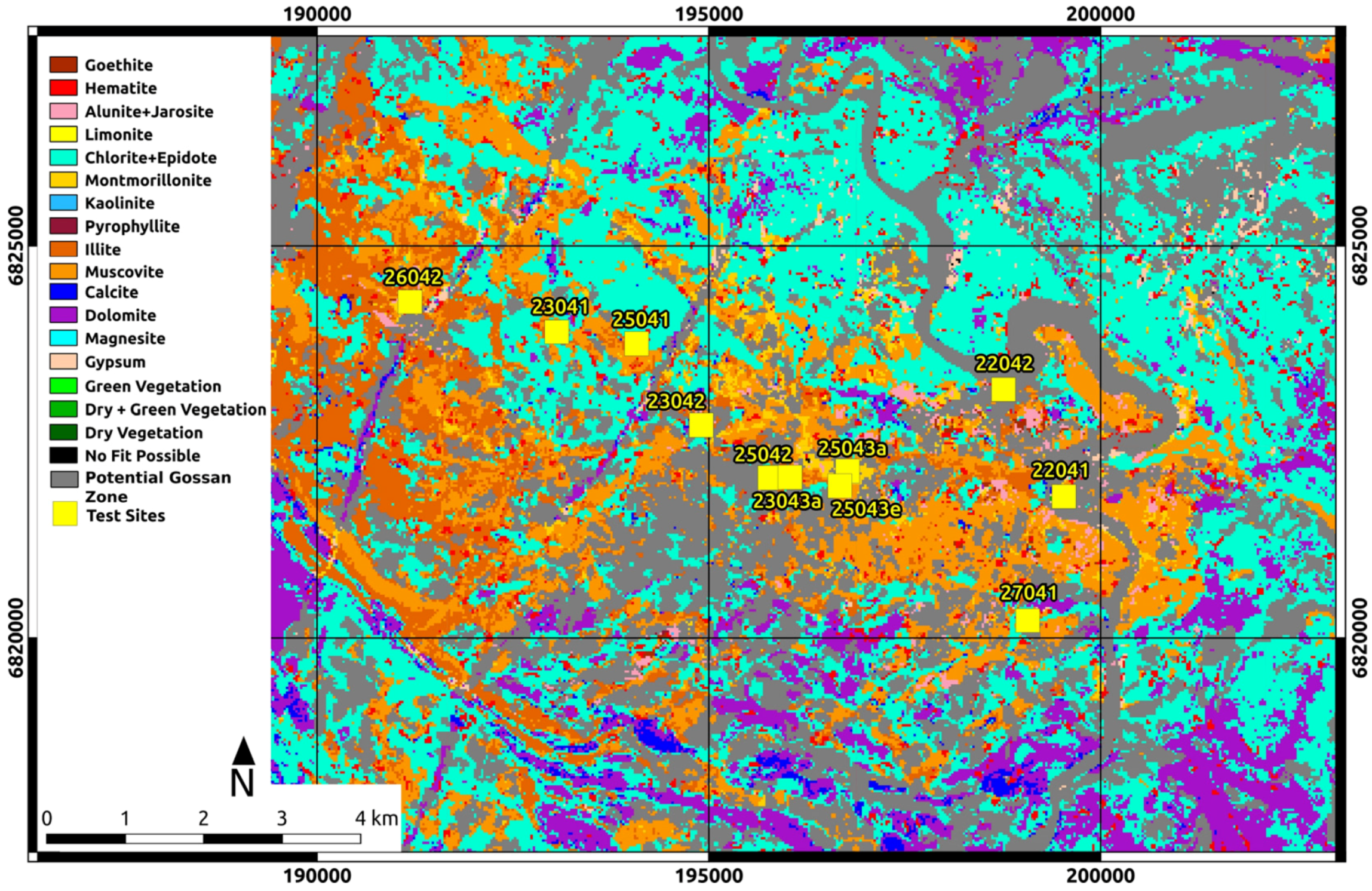
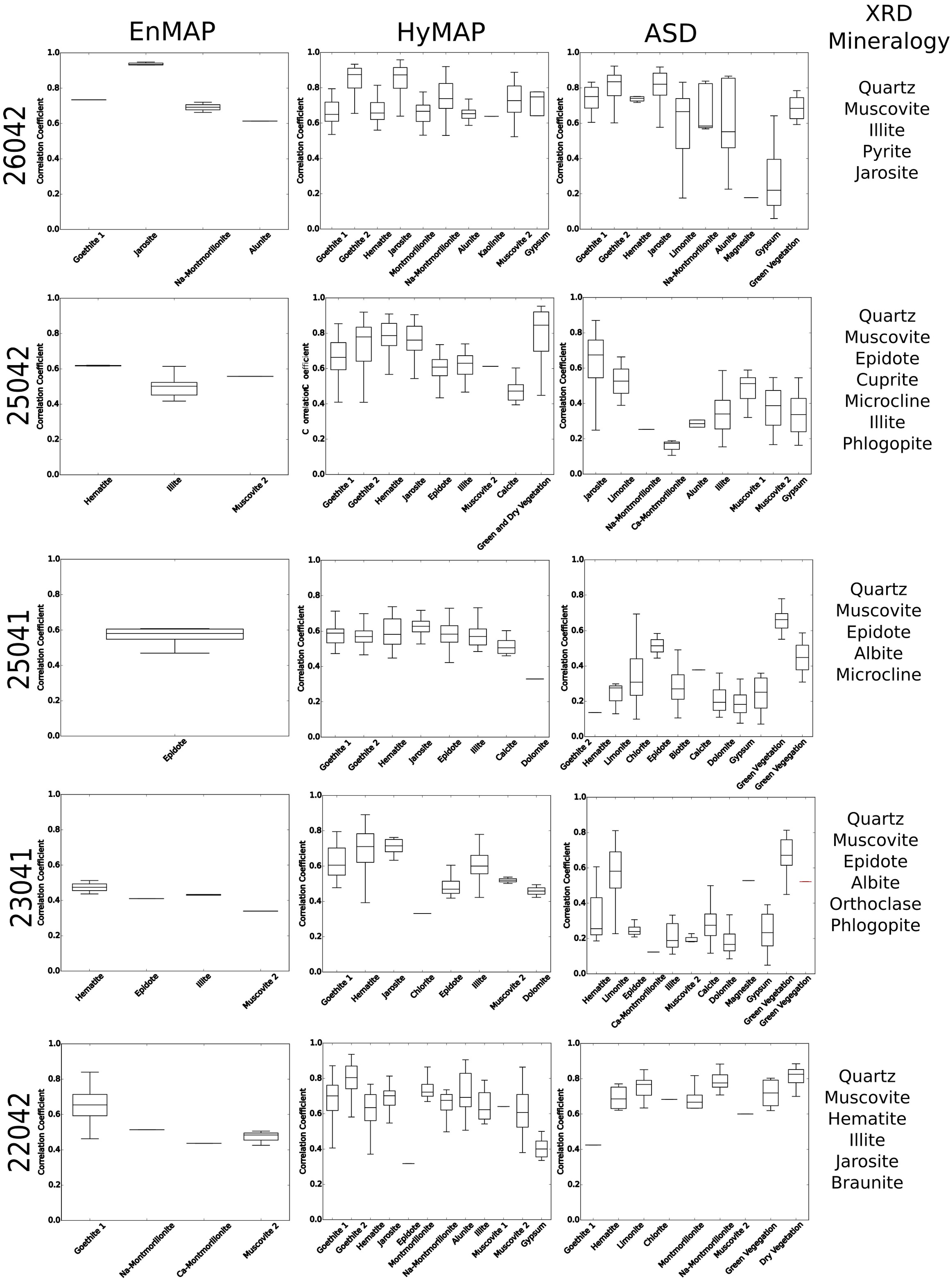
5.5.2. Haib River

The Haib river porphyry copper-molybdenum deposit shows characteristic gossan areas, which may outline potential exploration targets [53]. These zones are of specific economic interest as they have been identified as zones of potential low cost ore production [25]. The innermost zone of this leached capping [47] is a hematitic gossan, which is associated with a dominance of the copper-bearing sulfide mineral chalcopyrite over pyrite [46,47]. This zone grades outwards into a gossan zone which is dominated by goethite and further outwards into jarosite as already described above. Figure 19 shows the identified leached-capping exploration anomalies according to the gossan zonation and its characteristic mineralogy calculated from simulated EnMAP data. The gossan zones near the center of the mineralization are clearly visible as well as the gossan zone at 26042, which has also been described by previous multispectral work, using Sentinel-2, OLI and ALI data [53].

Figure 18. Location of the advanced argillic alteration centers, shown as grey opaque overlay, calculated from simulated EnMAP data.

Figure 18. Location of the advanced argillic alteration centers, shown as grey opaque overlay, calculated from simulated EnMAP data.

Figure 19. Location of the gossan zones, shown as grey opaque overlay, calculated from simulated EnMAP data.

Figure 19. Location of the gossan zones, shown as grey opaque overlay, calculated from simulated EnMAP data.

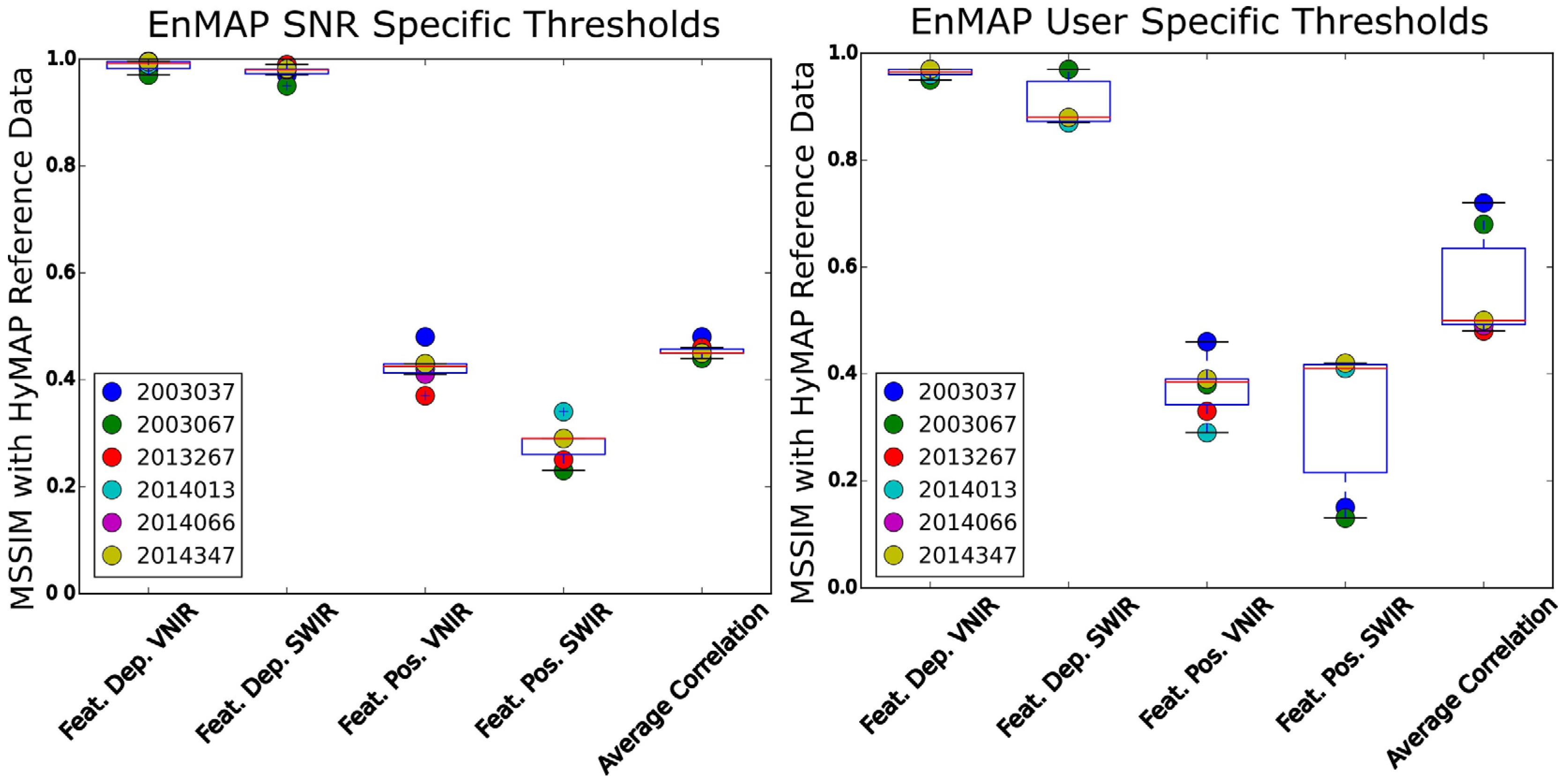
6. Performance of EnGeoMAP 2.0 for EnMAP Data

EnGeoMAP 2.0 can only be validated in a relative sense over the Haib River and the Rodalquilar areas considering the large size and rugged terrain of both mineral deposit sites. EnGeoMAP 2.0 results are calculated from the higher spatial resolution HyMAP data, which will serve as reference for testing the performance of EnGeoMAP 2.0. The higher spatially resolved results of the HyMAP data are median filtered with a 7 × 7 pixel median filter together with nearest neighbor resampling to 30 m. Now the EnGeoMAP 2.0 results of the HyMAP reference can be compared to the EnGeoMAP 2.0 results of simulated EnMAP data and Hyperion data. This can be done using the MSSIM [40] as comparison operator over an area with intersecting data coverage.

The three main criteria for performance assessment of EnGeoMAP 2.0 are spectral performance, spatial performance and material detection performance shown in Figure 20. These parameters are calculated from the ancillary information provided by EnGeoMAP 2.0. The spectral performance can be characterized by comparing the maximum absorption depths in the VNIR till 1000 nm and in SWIR from 1000 nm onwards. MSSIM values close to one indicate a near perfect preservation of the maximum absorption depth values due to the high sensitivity of the MSSIM towards noise, gain and offset differences between the reference HyMAP data and the comparison data (EnMAP) [40]. Performance data from Hyperion is shown in Supplement S5.3.

Figure 20. Comparison of the spectral (Feature Depth VNIR, Feature Depth SWIR), spatial (Feature Position VNIR, Feature Position SWIR) and material mapping performance (Average Correlation) at intersecting areas between simulated EnMAP data and the HyMAP reference data via the Mean Structural Similarity Index Measure. SNR specific thresholds depict the results from the sensor SNR specific EnGeoMAP 2.0 mapping approach, whilst the user specific thresholds depict the mapping results from fixed user defined absorption depth thresholds for the VNIR (2%) and the SWIR (3%).

Figure 20. Comparison of the spectral (Feature Depth VNIR, Feature Depth SWIR), spatial (Feature Position VNIR, Feature Position SWIR) and material mapping performance (Average Correlation) at intersecting areas between simulated EnMAP data and the HyMAP reference data via the Mean Structural Similarity Index Measure. SNR specific thresholds depict the results from the sensor SNR specific EnGeoMAP 2.0 mapping approach, whilst the user specific thresholds depict the mapping results from fixed user defined absorption depth thresholds for the VNIR (2%) and the SWIR (3%).

The spatial performance can be tested by comparing the position of the maximum absorption features in the VNIR and the SWIR between the spaceborne data and the HyMAP reference data that was resampled to a ground sampling distance of 30 m. Here complex material mixtures in the sub-30 m pixel domain (e.g., see Figure 10 and Figure 15) are the main cause for spatio-spectral gradients that alter the shape and hence the position of the maximum absorption features in the VNIR and the SWIR. The material mapping performance can be assessed by comparing the corresponding linear correlation coefficients to the library spectra between the HyMAP reference scene and EnMAP data through the MSSIM followed by an averaging of these MSSIM for each comparison site. The results are shown in Figure 20. Here we see that the maximum absorption depth preservation for the simulated EnMAP data in comparison to the HyMAP reference is always above 90%. The spatial performance of the EnGeoMAP 2.0 results calculated from simulated EnMAP data are on average 40%. The average material correlation between the HyMAP EnGeoMAP 2.0 reference results and the EnGeoMAP 2.0 results from simulated EnMAP data show that EnMAP reaches 50% material detection similarity to the reference.

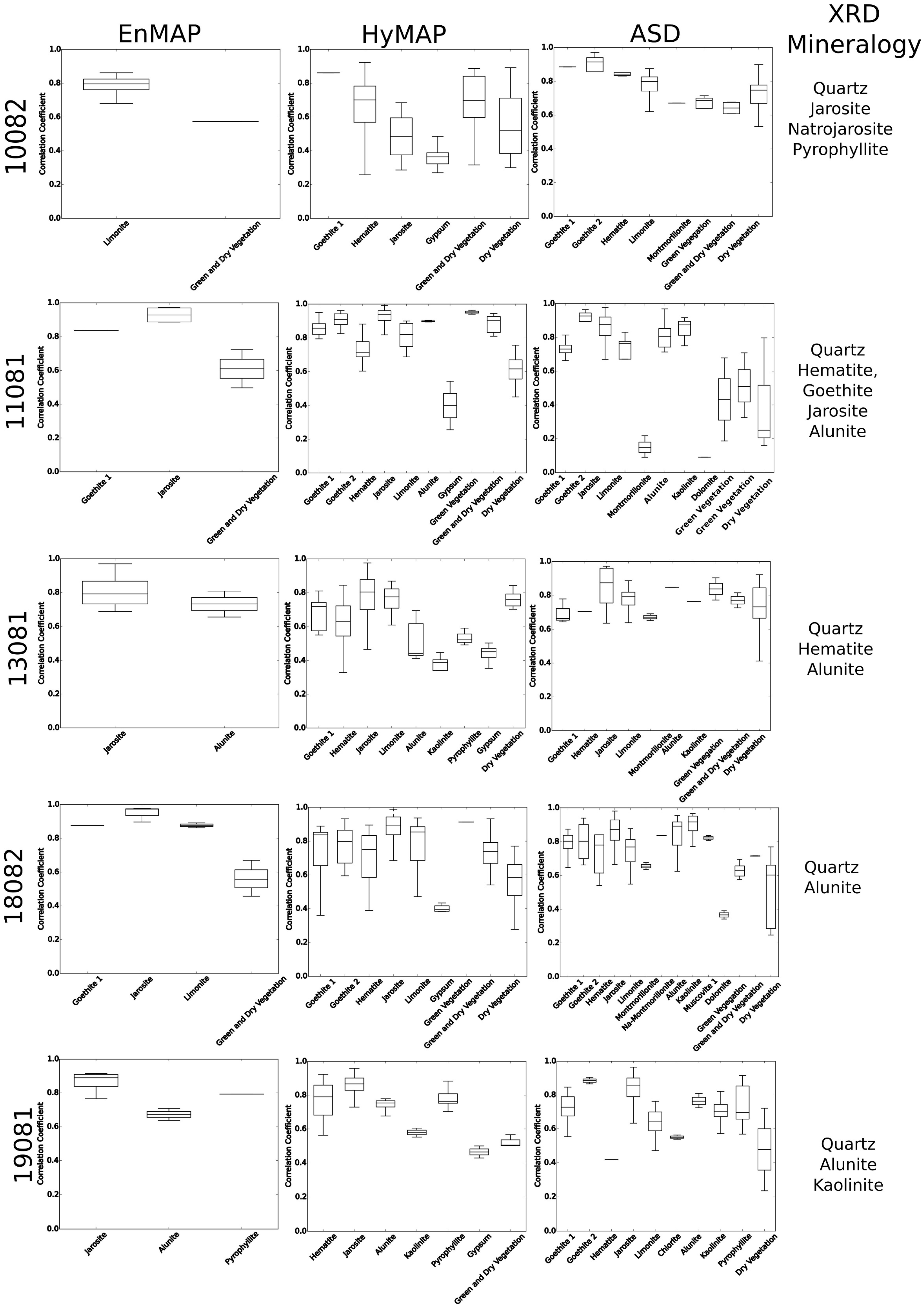
7. Validation

Validation has been carried out at test sites that have been visited in the field for in situ spectroscopic measurements together with surface samples that have been collected for later laboratory XRD analysis. The EnGeoMAP 2.0 results covering an area of 90 m by 90 m were clipped at each field site for the simulated EnMAP data and the HyMAP reference data. The analysis results are shown with their respective best correlation value at these field test sites. Figure 21 shows data from the Rodalquilar area, Figure 22 shows the data from the Haib River complex. These results are valid for the GFZ spectral library [36]. Results for the USGS spectral library and the mixed library [12] are shown in Supplement 6. The validation data shows the linear correlation coefficient data of identified material around each test site for EnGeoMAP 2.0 results calculated from ASD, HyMAP and simulated EnMAP data. This approach is similar to the intrinsic validation shown in van der Meer (2006) [41].

Figure 21 shows that jarosite, alunite and kaolinite can be found at the rock waste dump north of the Cinto mines (19081), which can also be seen in the XRD composition data. The test site 13081, situated near the Los Tollos alunite mine shows abundant alunite and jarosite, within the three spectroscopic datasets. This is verified by the presence of alunite in the XRD data. Test site 11081, situated at a prominent alunite jarosite outcrop, which has been described by Arribas et al., 1989 [21], shows abundant alunite and jarosite in the spectroscopic data and the XRD data as well. Verification data for EnGeoMAP 2.0 results of the Haib river area show a similar pattern. Here test site 26042, shows the characteristic gossan minerals goethite, hematite and jarosite in the spectroscopic data of HyMAP and the ASD field spectrometer. Jarosite is also found together with pyrite in the XRD data. The sample points 23041 and 25041 show abundant epidote and chlorite in the EnGeoMAP 2.0 results of the spectroscopic data, together with epidote in the XRD data. However, the correlation values of these minerals calculated from the simulated EnMAP data are only between 0.4 and 0.6. This is caused by the previously discussed overlap of the absorption features of chlorite, calcite and epidote [54] if synthetic mixtures are disregarded. Therefore, higher correlation values can be observed for linear combinations of multiple USGS reference spectra such as chlorite + epidote + calcite, or chlorite + muscovite, shown in Figure S18. The rather low correlation values for the ASD data in Figure 22 and Figure S18 can be attributed to an increased noise level in the spectral region beyond 2300 nm for the bare fiber spectra, as shown in Figure 3 (right). Data from the main mineralized zone of the Haib river area (25041 and 22042) show abundant muscovite in the spectral data and in the ASD reference data. These two specific compositions: (epidote, chlorite and calcite) and (quartz, muscovite, illite) reflect the two zones of the Haib river deposit described by Barr and Reid [25] and by Minnit [17]. More detailed fieldwork at the here presented mineral deposit sites and other field test sites worldwide need to be carried out to further validate EnGeoMAP 2.0. Here it was only possible to provide the validation results in the form of Figure 21 and Figure 22, as it was not possible to visit more field test sites in the time frame of the fieldwork.

Figure 21. Boxplots showing the linear correlation values of the EnGeoMAP 2.0 detected materials at field validation sites from the Rodalquilar area from simulated EnMAP data, HyMAP data and ASD field spectra together with analysis results from XRD data.

Figure 21. Boxplots showing the linear correlation values of the EnGeoMAP 2.0 detected materials at field validation sites from the Rodalquilar area from simulated EnMAP data, HyMAP data and ASD field spectra together with analysis results from XRD data.

Figure 22. Boxplots showing the linear correlation values of the EnGeoMAP 2.0 detected materials at field validation sites from the Haib River area from simulated EnMAP data, HyMAP data and ASD field spectra together with analysis results from XRD data.

Figure 22. Boxplots showing the linear correlation values of the EnGeoMAP 2.0 detected materials at field validation sites from the Haib River area from simulated EnMAP data, HyMAP data and ASD field spectra together with analysis results from XRD data.

8. Conclusions and Outlook

The work presented here shows that EnGeoMAP 2.0 adds four aspects to the automated analysis of imaging spectroscopy data with expert systems.

• It is able to produce material maps using the geometric hull automated absorption feature definition, which requires no a priori knowledge about the shape of the reference library spectra or the image spectra [14]. This is different to the fixed defined features of part of the USGS Tetracorder or MICA [9,10].
• The EnGeoMAP 2.0 algorithm is able to incorporate sensor specific SNR information. Otherwise user defined minimum absorption depths for VNIR and SWIR absorption features may be used.
• The calculation of spatio-spectral gradients of e.g., EnMAP data is possible by hyperspectral gradient detection [32]. It may be used to outline areas of high spatial material heterogeneity. These areas may otherwise only be resolved by calculating material maps from cost intensive hyperspectral airborne image scenes.
• EnGeoMAP 2.0 includes the automatic detection of mineral anomalies (e.g., gossans or hydrothermal alteration zones), which is not part of the USGS Tetracorder or MICA [9,10] in the form described here.

EnGeoMAP 2.0 widens the user base of hyperspectral data and data products to more end-users. This enables exploration geologists and consultants in geoscience to facilitate these ready-to-use mineral maps and exploration anomaly maps without an explicit in-depth knowledge of imaging spectroscopy.

Simulated EnMAP data has shown the great potential of the EnMAP mission to characterize mineral deposit sites and to highlight exploration anomalies via spaceborne hyperspectral data using the here presented EnGeoMAP 2.0 algorithm. EnMAP significantly outperforms the currently available Hyperion sensor in characterizing the surface mineralogy at the mineral deposit sites of Rodalquilar and Haib River.

Although Hyperion shows the least potential for mineral mapping it still is a very useful spaceborne sensor for automated mineral mapping using, as it is to date the only available spaceborne imaging spectrometer covering also the SWIR spectral range.

Future versions of EnGeoMAP may be extended by an incorporation of thermal infrared data into the analysis process together with more mineral deposit models for exploration anomaly characterization.

References

- Middleton, E.M.; Ungar, S.G.; Mandl, D.J.; Ong, L.; Frye, S.W.; Campbell, P.E.; Landis, D.R.; Young, J.P.; Pollack, N.H. The earth observing one (EO-1) satellite mission: Over a decade in space. IEEE J. Sel. Top. Appl. Earth Obs. Remote Sens. 2013, 6, 243–256. [Google Scholar] [CrossRef]
- Cocks, T.; Jenssen, R.; Stewart, A.; Wilson, I.; Shields, T. The HyMapTM airborne hyperspectral sensor: The system, calibration and performance. In Proceedings of the 1st EARSeL Workshop on Imaging Spectroscopy, Zurich, Switzerland, 6–8 October 1998; pp. 37–42.
- Baarstad, I.; Løke, T.; Kaspersen, P. ASI–A new airborne hyperspectral imager. In Proceedings of the 4th EARSeL Workshop on Imaging Spectroscopy, Warsaw, Poland, 27–29 April 2005; pp. 107–110.
- Mielke, C.; Rogass, C.; Boesche, N.K.; Segl, K.; Kaufmann, H. Multi- and hyperspectral satellite sensors for mineral exploration, new applications to the Sentinel-2 and EnMAP mission. In Proceedings of the EARSeL 34th Symposium Proceedings, Warsaw, Poland, 16–20 June 2014. [CrossRef]
- Kopačková, V. Using multiple spectral feature analysis for quantitative pH mapping in a mining environment. Int. J. Appl. Earth Obs. Geoinform. 2014, 28, 28–42. [Google Scholar] [CrossRef]
- Swayze, G.A.; Smith, K.S.; Clark, R.N.; Sutley, S.J.; Pearson, R.M.; Vance, J.S.; Hageman, P.L.; Briggs, P.H.; Meier, A.L.; Singleton, M.J.; et al. Using imaging spectroscopy to map acidic mine waste. Environ. Sci. Technol. 2000, 34, 47–54. [Google Scholar] [CrossRef]
- Guanter, L.; Kaufmann, H.; Segl, K.; Foerster, S.; Rogass, C.; Chabrillat, S.; Kuester, T.; Hollstein, A.; Rossner, G.; Chlebek, C.; et al. The EnMAP spaceborne imaging spectroscopy mission for earth observation. Remote Sens. 2015, 7, 8830–8857. [Google Scholar] [CrossRef]
- Iwasaki, A.; Ohgi, N.; Tanii, J.; Kawashima, T.; Inada, H. Hyperspectral Imager Suite (HISUI)—Japanese hyper-multi spectral radiometer. In Proceedings of the 2011 IEEE International Geoscience and Remote Sensing Symposium (IGARSS), Vancouver, BC, Canada, 24–29 July 2011; pp. 1025–1028.
- Clark, R.N.; Swayze, G.A.; Livo, K.E.; Kokaly, R.F.; Sutley, S.J.; Dalton, J.B.; McDougal, R.R.; Gent, C.A. Imaging spectroscopy: Earth and planetary remote sensing with the USGS Tetracorder and expert systems. J. Geophys. Res. Planets 2003, 108. [Google Scholar] [CrossRef]
- Kokaly, R.F. Spectroscopic remote sensing for material identification, vegetation characterization, and mapping. Proc. SPIE 2012, 8390. [Google Scholar] [CrossRef]
- Kokaly, R.F.; King, T.V.V.; Livo, K.E. Airborne Hyperspectral. Survey of Afghanistan 2007: Flight Line Planning and HyMAP Data Collection; Open File Report; United States Geological Survey: Reston, VA, USA, 2008. [Google Scholar]
- Clark, R.N.; Swayze, G.A.; Wise, R.; Livo, E.; Hoefen, T.M.; Kokaly, R.F.; Sutley, S.J. USGS Digital Spectral Library Splib06a; Geological Survey Data Series 231; U.S. Geological Survey: Denver, CO, USA, 2007.
- Rogass, C.; Segl, K.; Mielke, C.; Fuchs, Y. EnGeoMAP—A geological mapping tool applied to the EnMAP mission. EARSeL EProc. 2013, 12, 94–100. [Google Scholar]
- Mielke, C.; Boesche, N.K.; Rogass, C.; Kaufmann, H.; Gauert, C. New geometric hull continuum removal algorithm for automatic absorption band detection from spectroscopic data. Remote Sens. Lett. 2015, 6, 97–105. [Google Scholar] [CrossRef]
- Segl, K.; Guanter, L.; Rogass, C.; Kuester, T.; Roessner, S.; Kaufmann, H.; Sang, B.; Mogulsky, V.; Hofer, S. EeteS the EnMAP end-to-end simulation tool. IEEE J. Sel. Top. Appl. Earth Obs. Remote Sens. 2012, 5, 522–530. [Google Scholar] [CrossRef]
- Arribas, A.; Cunningham, C.G.; Rytuba, J.J.; Rye, R.O.; Kelly, W.C.; Podwysocki, M.H.; McKee, E.H.; Tosdal, R.M. Geology, geochronology, fluid inclusions, and isotope geochemistry of the Rodalquilar gold alunite deposit, Spain. Econ. Geol. 1995, 90, 795–822. [Google Scholar] [CrossRef]
- Minnitt, R.C.A. Porphyrry Copper-Molybdenium Mineralization at Haib River, South West Africa/Namibia. In Mineral Deposits of Southern Africa; Anhaeusser, C.R., Maske, S., Eds.; Geological Society of South Africa: Johannesburg, South Africa, 1986; Volume 2, pp. 1567–1585. [Google Scholar]
- Rogass, C.; Mielke, C.; Scheffler, D.; Boesche, N.K.; Lausch, A.; Lubitz, C.; Brell, M.; Spengler, D.; Eisele, A.; Segl, K.; et al. Reduction of uncorrelated striping noise—Applications for hyperspectral pushbroom acquisitions. Remote Sens. 2014, 6, 11082–11106. [Google Scholar] [CrossRef]
- Pearlman, J.S. Hyperion Validation Report; Boeing Report; Phantom Works, The Boeing Company: Kent, WA, USA, 2003. [Google Scholar]
- Van der Meer, F.D.; van der Werff, H.; van Ruitenbeek, F.J.A.; Hecker, C.A.; Bakker, W.H.; Noomen, M.F.; van der Meijde, M.; Carranza, E.J.M.; Smeth, J.; Woldai, T. Multi-and hyperspectral geologic remote sensing: A review. Int. J. Appl. Earth Obs. Geoinform. 2012, 14, 112–128. [Google Scholar] [CrossRef]
- Arribas, A., Jr.; Rytuba, J.J.; Rye, R.O.; Cunningham, C.G.; Podwysocki, M.H.; Kelly, W.C.; Arribas, A.S.; McKee, E.H.; Smith, J.G. Preliminary Study of the Ore Deposits and Hydrothermal Alteration in the Rpdalquilar. Caldera Complex, Southeastern Spain; USGS Open-File Report; United States Geological Survey: Reston, VA, USA, 1989.
- Rytuba, J.J.; Arribas, A.A.; Cunningham, C.G.; McKee, E.H.; Podwysocki, M.H.; Smith, J.G.; Kelly, W.C.; Arribas, A. Mineralized and unmineralized calderas in Spain; Part II, evolution of the Rodalquilar caldera complex and associated gold-alunite deposits. Miner. Depos. 1990, 25, S29–S35. [Google Scholar] [CrossRef]
- Cunningham, C.G.; Arribas, A.; Rytuba, J.J. Mineralized and unmineralized calderas in Spain; Part I, evolution of the Los Frailes Caldera. Miner. Depos. 1990, 25, S21–S28. [Google Scholar] [CrossRef]
- Pirajno, F. Hydrothermal Processes and Mineral Systems; Springer-Verlag: Berlin, Germany, 2009. [Google Scholar]
- Barr, J.M.; Reid, D.L. Hydrothermal alteration at the Haib porphyry copper deposit, Namibia: Stable isotope and fluid inclusion patterns. Communs. Geol. Surv. Namib. 1993, 8, 23–34. [Google Scholar]
- Schläpfer, D.; Richter, R. Geo-atmospheric processing of airborne imaging spectrometry data. Part 1: Parametric orthorectification. Int. J. Remote Sens. 2002, 23, 2609–2630. [Google Scholar] [CrossRef]
- Richter, R.; Schläpfer, D. Geo-atmospheric processing of airborne imaging spectrometry data. Part 2: Atmospheric/topographic correction. Int. J. Remote Sens. 2002, 23, 2631–2649. [Google Scholar] [CrossRef]
- Rogass, C.; Guanter, L.; Mielke, C.; Scheffler, D.; Boesche, N.K.; Lubitz, C.; Brell, M.; Spengler, D.; Segl, K. An automated processing chain for the retrieval of georeferenced reflectance data from hyperspectral EO-1 Hyperion acquisitions. In Proceedings of the EARSeL 34th Symposium Proceedings, Warsaw, Poland, 16–20 June 2014. [CrossRef]
- Van der Linden, S.; Rabe, A.; Held, M.; Jakimow, B.; Leitão, P.; Okujeni, A.; Schwieder, M.; Suess, S.; Hostert, P. The EnMAP-Box—A toolbox and application programming interface for EnMAP data processing. Remote Sens. 2015, 7, 11249–11266. [Google Scholar] [CrossRef]
- Storch, T.; De Miguel, A.; Müller, R.; Müller, A.; Neumann, A.; Walzel, T.; Bachmann, M.; Palubinskas, G.; Lehner, M.; Richter, R.; et al. The future spaceborne hyperspectral imager EnMAP: Its calibration, validation, and processing chain. In Proceedings of the 21st Congress International Society for Photogrammetry and Remote Sensing, Beijing, China, 3–11 July 2008; pp. 1265–1270.
- Bakker, W.H.; Schmidt, K.S. Hyperspectral edge filtering for measuring homogeneity of surface cover types. ISPRS J. Photogramm. Remote Sens. 2002, 56, 246–256. [Google Scholar] [CrossRef]
- Rogaß, C.; Itzerott, S.; Schneider, B.U.; Kaufmann, H.; Hüttl, R.F. Hyperspectral boundary detection based on the busyness multiple correlation edge detector and alternating vector field convolution snakes. ISPRS J. Photogramm. Remote Sens. 2010, 65, 468–478. [Google Scholar] [CrossRef]
- Hunt, J.M.; Turner, D.S. Determination of mineral constituents of rocks by infrared spectroscopy. Anal. Chem. 1953, 25, 1169–1174. [Google Scholar] [CrossRef]
- Hunt, G.R.; Ashley, R.P. Spectra of altered rocks in the visible and near infrared. Econ. Geol. 1979, 74, 1613–1629. [Google Scholar] [CrossRef]
- Townsend, T.E. Discrimination of iron alteration minerals in visible and near-infrared reflectance data. J. Geophys. Res. Solid Earth 1987, 92, 1441–1454. [Google Scholar] [CrossRef]
- Papenfuß, A. Detection of Copper Deposits Based on a New Spectral Library Using Imaging Spectroscopy. Master’s Thesis, Universität Potsdam, Potsdam, Germany, 2015. [Google Scholar]
- Gao, L.; Du, Q.; Zhang, B.; Yang, W.; Wu, Y. A comparative study on linear regression-based noise estimation for hyperspectral imagery. IEEE J. Sel. Top. Appl. Earth Obs. Remote Sens. 2013, 6, 488–498. [Google Scholar] [CrossRef]
- Oshigami, S.; Yamaguchi, Y.; Uezato, T.; Momose, A.; Arvelyna, Y.; Kawakami, Y.; Yajima, T.; Miyatake, S.; Nguno, A. Mineralogical mapping of southern Namibia by application of continuum-removal MSAM method to the HyMap data. Int. J. Remote Sens. 2013, 34, 5282–5295. [Google Scholar] [CrossRef]
- Du, Y.; Chang, C.-I.; Ren, H.; Chang, C.-C.; Jensen, J.O.; D’Amico, F.M. New hyperspectral discrimination measure for spectral characterization. Opt. Eng. 2004, 43, 1777–1786. [Google Scholar]
- Wang, Z.; Bovik, A.C.; Sheikh, H.R.; Simoncelli, E.P. Image quality assessment: From error visibility to structural similarity. IEEE Trans. Image Process. 2004, 13, 600–612. [Google Scholar] [CrossRef] [PubMed]
- Van der Meer, F. The effectiveness of spectral similarity measures for the analysis of hyperspectral imagery. Int. J. Appl. Earth Obs. Geoinform. 2006, 8, 3–17. [Google Scholar] [CrossRef]
- Quintano, C.; Fernández-Manso, A.; Shimabukuro, Y.E.; Pereira, G. Spectral unmixing. Int. J. Remote Sens. 2012, 33, 5307–5340. [Google Scholar] [CrossRef]
- Canny, J. A Computational approach to edge detection. IEEE Trans. Pattern Anal. Mach. Intell. 1986, PAMI-8, 679–698. [Google Scholar] [CrossRef]
- Swayze, G.A.; Clark, R.N.; Goetz, A.F.H.; Livo, K.E.; Breit, G.N.; Kruse, F.A.; Sutley, S.J.; Snee, L.W.; Lowers, H.A.; Post, J.L.; et al. Mapping advanced argillic alteration at Cuprite, Nevada, using imaging spectroscopy. Econ. Geol. 2014, 109, 1179–1221. [Google Scholar] [CrossRef]
- King, T.V.V.; Berger, B.R.; Johnson, M.R. Characterization of Potential Mineralization in Afghanistan: Four Permissive Areas Identified Using Imaging Spectroscopy Data; USGS Open-File Report; United States Geological Survey: Reston, VA, USA, 2014.
- Chavez, W.X., Jr. Supergene oxidation of copper deposits: Zoning and distribution of copper oxide minerals. Soc. Econ. Geol. Newsl. 2000, 41, 9–21. [Google Scholar]
- Taylor, R. Gossans and Leached Cappings—Field Assessment, 1st ed.; Springer: Berlin, Germany, 2011. [Google Scholar]
- Haralick, R.M.; Sternberg, S.R.; Zhuang, X. Image analysis using mathematical morphology. IEEE Trans. Pattern Anal. Mach. Intell. 1987, PAMI-9, 532–550. [Google Scholar] [CrossRef]
- Bedini, E.; van der Meer, F.; van Ruitenbeek, F. Use of HyMap imaging spectrometer data to map mineralogy in the Rodalquilar caldera, southeast Spain. Int. J. Remote Sens. 2009, 30, 327–348. [Google Scholar] [CrossRef]
- Richter, N. Pedogenic Iron Ocide Determination of Soil Surfaces from Laboratory Spectra and HyMAP Image Data. A Case Study in the Cabo de Gata-Nijar Natural Park, SE Spain. Ph.D. Thesis, Humboldt-Universität zu Berlin, Berlin, Germany, 2010. [Google Scholar]
- Irons, J.R.; Dwyer, J.L.; Barsi, J.A. The next Landsat satellite: The Landsat data continuity mission. Remote Sens. Environ. 2012, 122, 11–21. [Google Scholar] [CrossRef]
- Drusch, M.; Del Bello, U.; Carlier, S.; Colin, O.; Fernandez, V.; Gascon, F.; Hoersch, B.; Isola, C.; Laberinti, P.; Martimort, P.; et al. Sentinel-2: ESA’s optical high-resolution Mission for GMES operational services. Remote Sens. Environ. 2012, 120, 25–36. [Google Scholar] [CrossRef]
- Mielke, C.; Boesche, N.K.; Rogass, C.; Segl, K.; Gauert, C.; Kaufmann, H. Potential applications of the Sentinel-2 multispectral sensor and the EnMAP hyperspectral sensor in mineral exploration. EARSeL EProc. 2014, 13, 93–102. [Google Scholar]
- Dalton, J.B.; Bove, D.J.; Mladinich, C.S.; Rockwell, B.W. Identification of spectrally similar materials using the USGS Tetracorder algorithm: The calcite–epidote–chlorite problem. Remote Sens. Environ. 2004, 89, 455–466. [Google Scholar] [CrossRef]
- Arribas, A. Characteristics of high-sulfidation epithermal deposits, and their relation to magmatic fluid. Mineral. Assoc. Can. Short Course 1995, 23, 419–454. [Google Scholar]
© 2016 by the authors; licensee MDPI, Basel, Switzerland. This article is an open access article distributed under the terms and conditions of the Creative Commons by Attribution (CC-BY) license (http://creativecommons.org/licenses/by/4.0/).
Share and Cite
Mielke, C.; Rogass, C.; Boesche, N.; Segl, K.; Altenberger, U. EnGeoMAP 2.0—Automated Hyperspectral Mineral Identification for the German EnMAP Space Mission. Remote Sens. 2016, 8, 127. https://doi.org/10.3390/rs8020127
Mielke C, Rogass C, Boesche N, Segl K, Altenberger U. EnGeoMAP 2.0—Automated Hyperspectral Mineral Identification for the German EnMAP Space Mission. Remote Sensing. 2016; 8(2):127. https://doi.org/10.3390/rs8020127
Chicago/Turabian StyleMielke, Christian, Christian Rogass, Nina Boesche, Karl Segl, and Uwe Altenberger. 2016. "EnGeoMAP 2.0—Automated Hyperspectral Mineral Identification for the German EnMAP Space Mission" Remote Sensing 8, no. 2: 127. https://doi.org/10.3390/rs8020127