
Efficient Emulation of Radiative Transfer Codes Using Gaussian Processes and Application to Land Surface Parameter Inferences


Abstract
:
1. Introduction
2. Gaussian Process Emulator
Extension to Full Spectrum Emulation
3. GP Emulation Examples
3.1. Emulating Soil-Leaf-Canopy RT Models

| Parameter | Symbol | Units | Minimum | Maximum | Transformation | Transformed Min | Transformed Max |
|---|---|---|---|---|---|---|---|
| Leaf layers | xleafn | – | 0.8 | 2.5 | – | – | – |
| Leaf chlorophyll
concentration | Cab | μ g·cm | 0.2 | 77 | 0.46 | 1 | |
| Leaf carotenoid concentration | Car | μ g·cm | 0 | 15 | 0.95 | 1 | |
| Senescent fraction | Csen | – | 0 | 1 | – | – | – |
| Equivalent water thickness | Cw | cm | 0.0043 | 0.0753 | 0.028 | 0.81 | |
| Leaf dry matter | Cm | g·cm | 0.0017 | 0.0331 | 0.037 | 0.84 | |
| Leaf area index | LAI | m ·m | 0 | 8 | 0.05 | 1 | |
| Average Leaf Angle | ALA | 0 | 90 | 0.44 | 0.56 | ||
| Soil brightness scalar | Bs | – | 0 | 2 | – | – | – |
| Soil moisture endmember | Ps | – | 0 | 1 | – | – | – |
| Weight of the first Price function | P1 | – | −0.5 | 1 | – | – | – |
| Weight of the second Price function | P2 | – | −0.5 | 1 | – | – | – |
| MODIS Band | Slope | Intercept | R | RMSE | MAE |
|---|---|---|---|---|---|
| 1 | 1.002 | 1.222e-05 | 0.9995 | 9.774e-04 | 5.175e-03 |
| 2 | 0.999 | 1.562e-04 | 0.9998 | 5.602e-04 | 1.063e-02 |
| 3 | 1.004 | −3.362e-05 | 0.9996 | 9.181e-04 | 2.371e-03 |
| 4 | 1.000 | 2.784e-05 | 0.9999 | 5.255e-04 | 2.048e-03 |
| 5 | 0.993 | 1.591e-03 | 0.9990 | 1.437e-03 | 3.588e-02 |
| 6 | 0.998 | 4.182e-04 | 0.9995 | 9.490e-04 | 1.587e-02 |
| 7 | 1.000 | 1.183e-04 | 0.9997 | 8.194e-04 | 1.135e-02 |


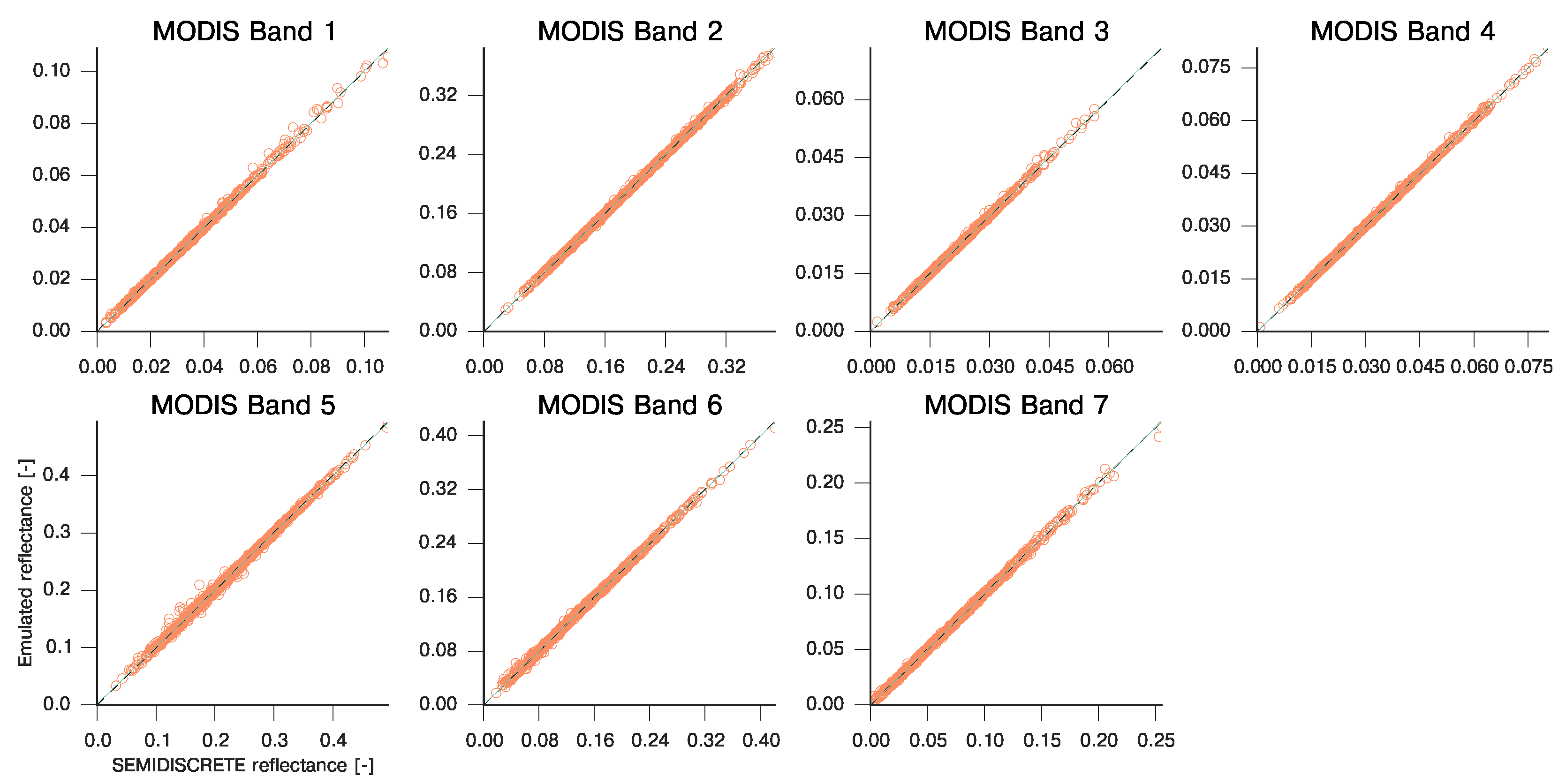
| MODIS Band | Slope | Intercept | R | RMSE | MAE |
|---|---|---|---|---|---|
| 1 | 0.984 | 0.000 | 0.999 | 1.669e-03 | 3.679e-02 |
| 2 | 1.000 | −0.000 | 1.000 | 2.681e-04 | 1.307e-02 |
| 3 | 0.947 | 0.001 | 0.990 | 4.349e-03 | 4.678e-02 |
| 4 | 0.977 | 0.001 | 0.998 | 1.987e-03 | 5.585e-02 |
| 5 | 1.001 | −0.000 | 1.000 | 3.523e-04 | 1.722e-02 |
| 6 | 1.000 | 0.000 | 1.000 | 3.210e-04 | 7.791e-03 |
| 7 | 1.000 | 0.000 | 1.000 | 2.416e-04 | 2.392e-03 |
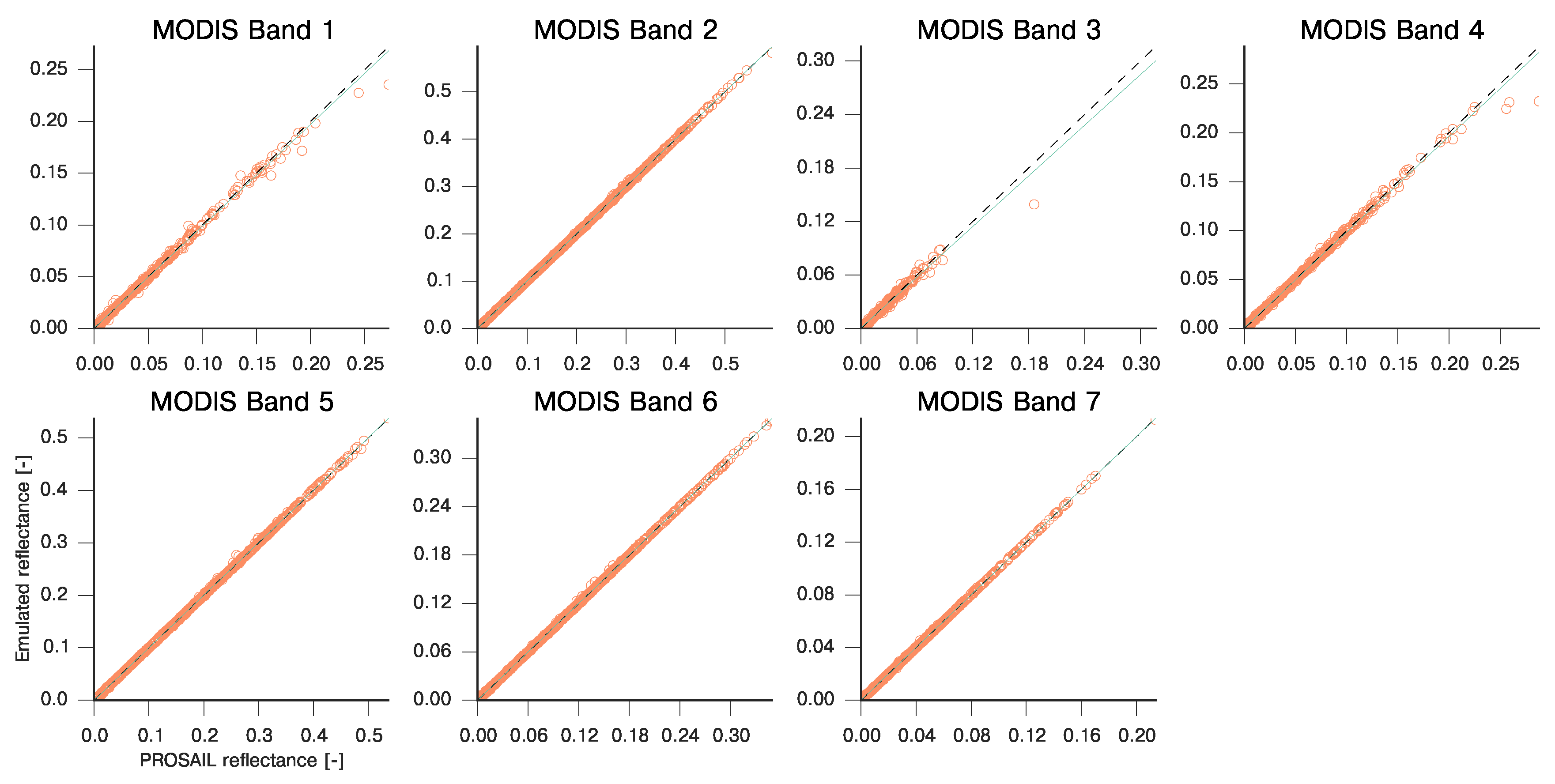
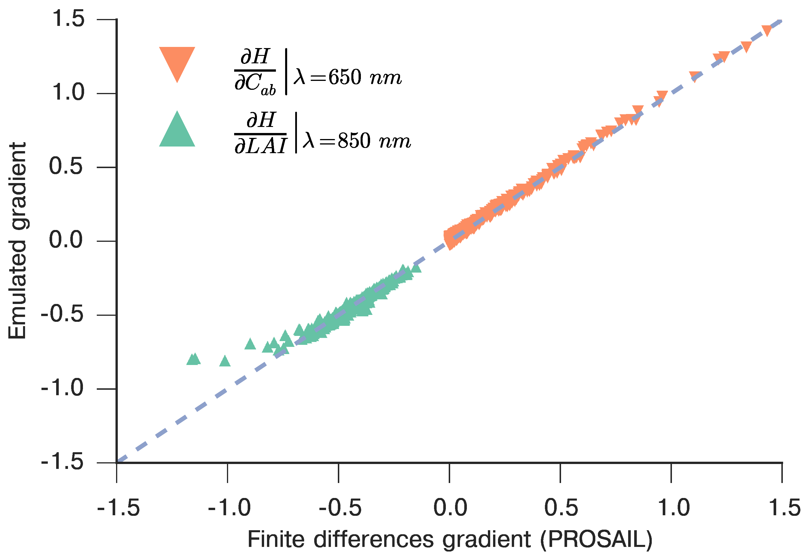
3.2. Emulation of a Coupled Soil-Leaf-Canopy-Atmosphere RT Model Combination: PROSAIL and 6S
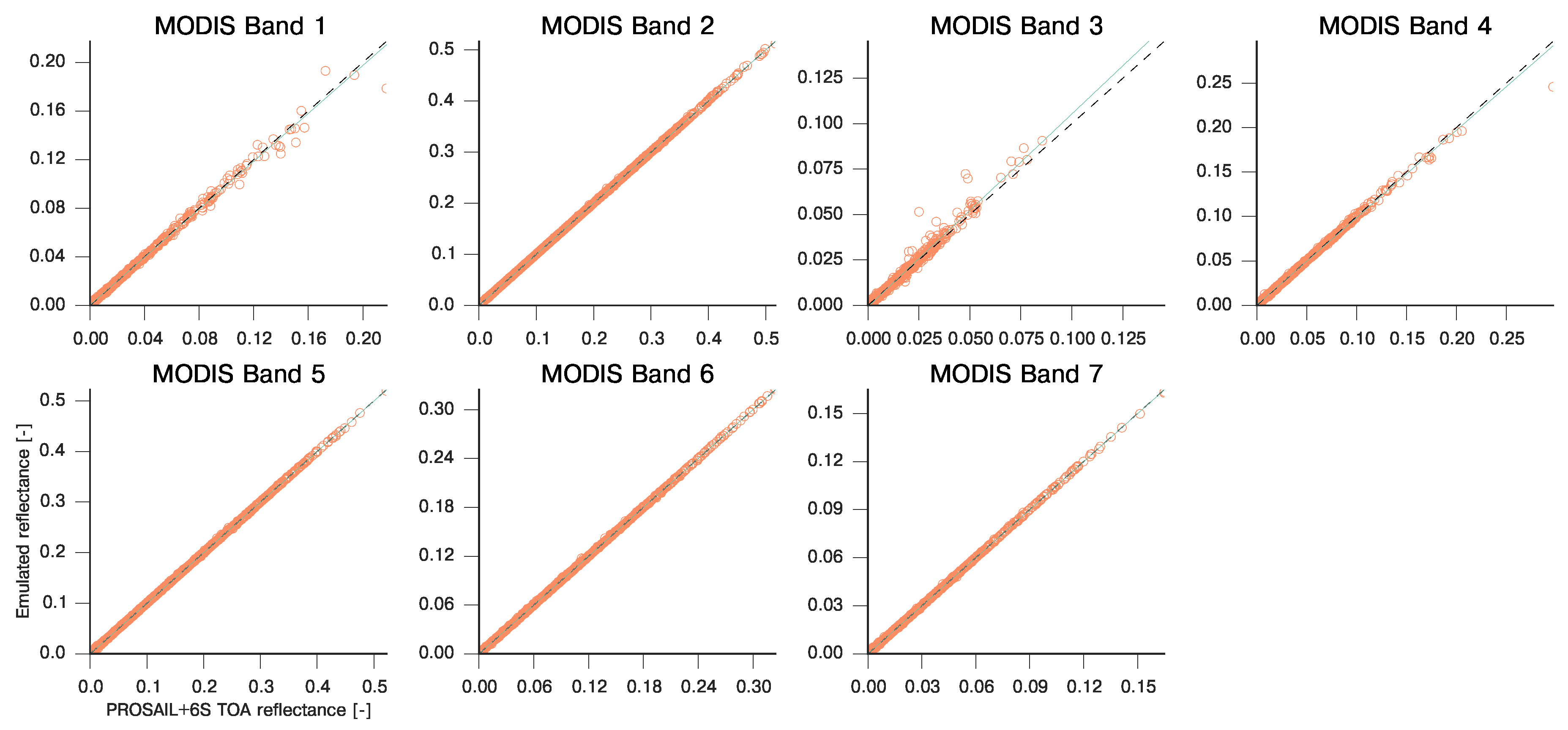
| MODIS Band | Slope | Intercept | R | RMSE | MAE |
|---|---|---|---|---|---|
| 1 | 0.985 | 0.000 | 0.998 | 2.087e-03 | 3.889e-02 |
| 2 | 1.001 | −0.000 | 1.000 | 1.888e-04 | 5.694e-03 |
| 3 | 1.061 | −0.001 | 0.989 | 4.996e-03 | 2.635e-02 |
| 4 | 0.981 | 0.001 | 0.998 | 1.730e-03 | 5.136e-02 |
| 5 | 0.999 | 0.000 | 1.000 | 2.282e-04 | 5.256e-03 |
| 6 | 1.000 | 0.000 | 1.000 | 2.342e-04 | 4.954e-03 |
| 7 | 0.999 | 0.000 | 1.000 | 2.885e-04 | 1.857e-03 |
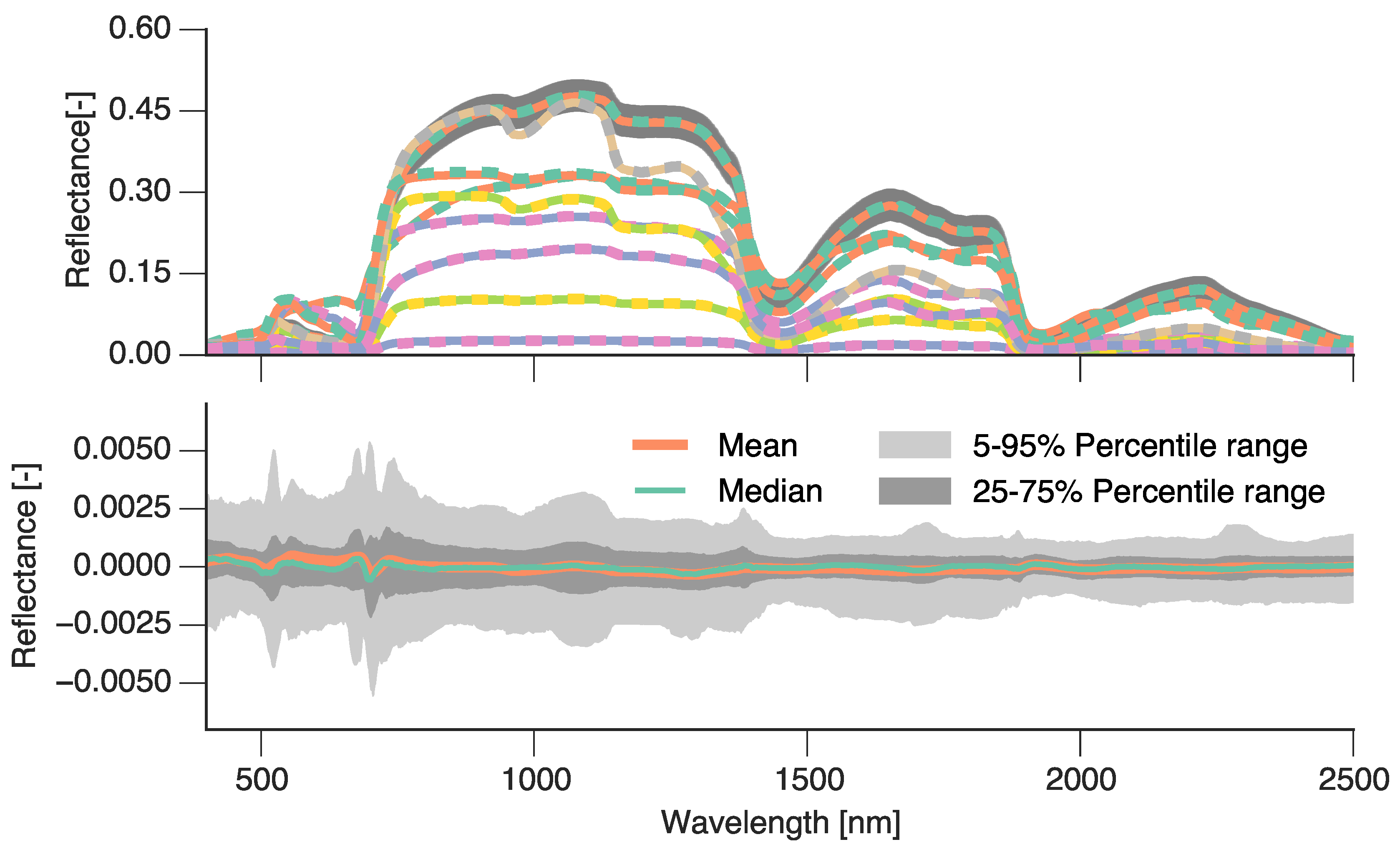
3.3. Spectral Emulation of a Coupled Soil-Leaf-Canopy RT Model Combination
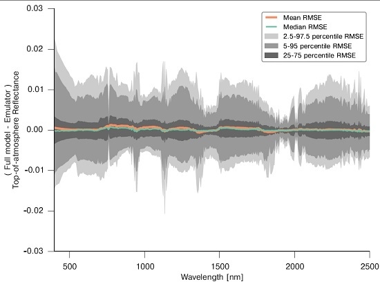
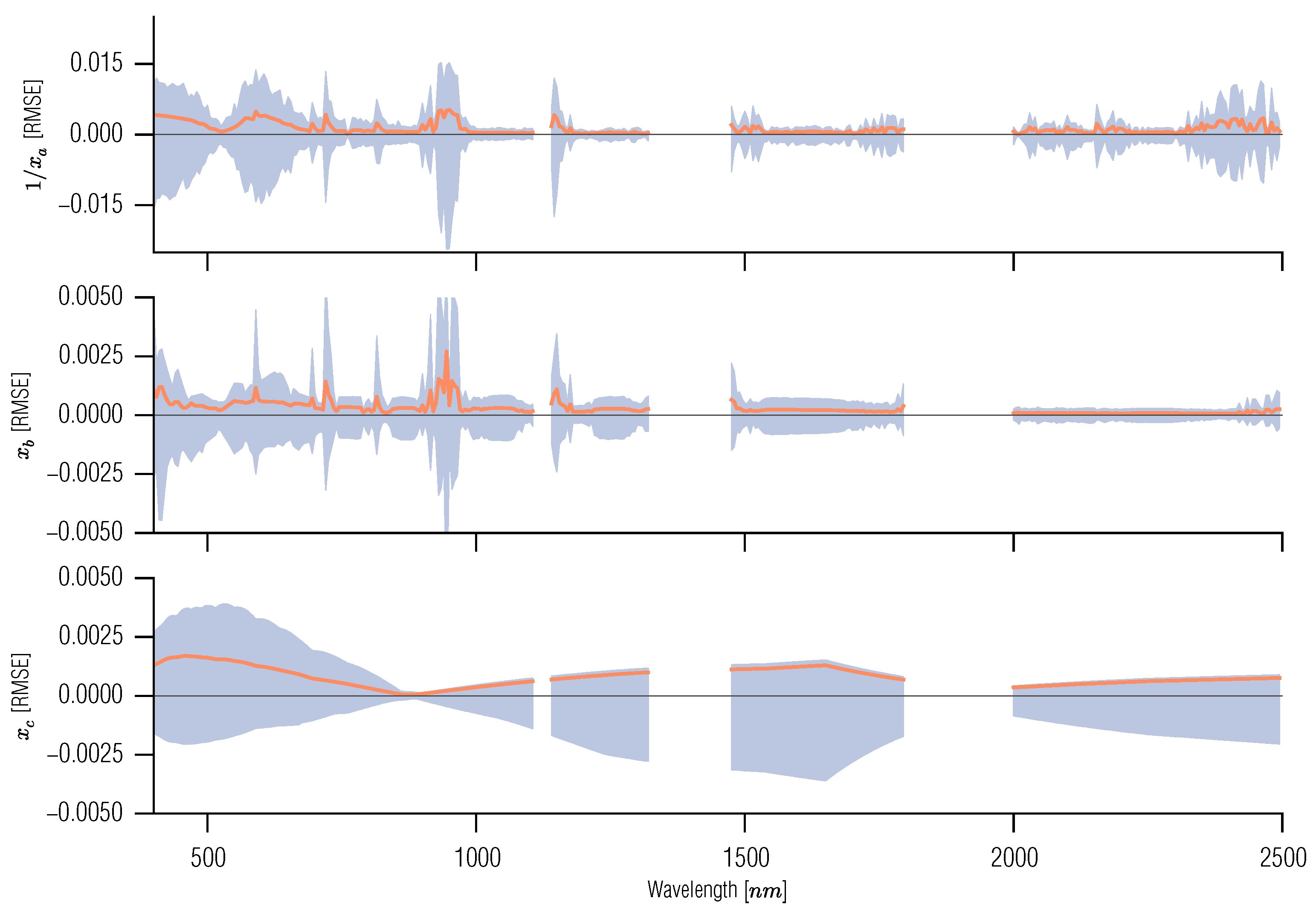
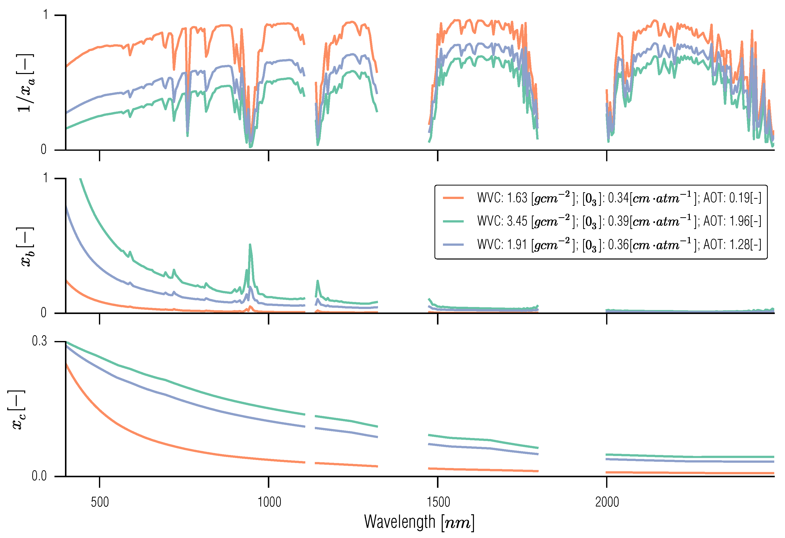
3.4. Spectral Emulation of Atmospheric Effects
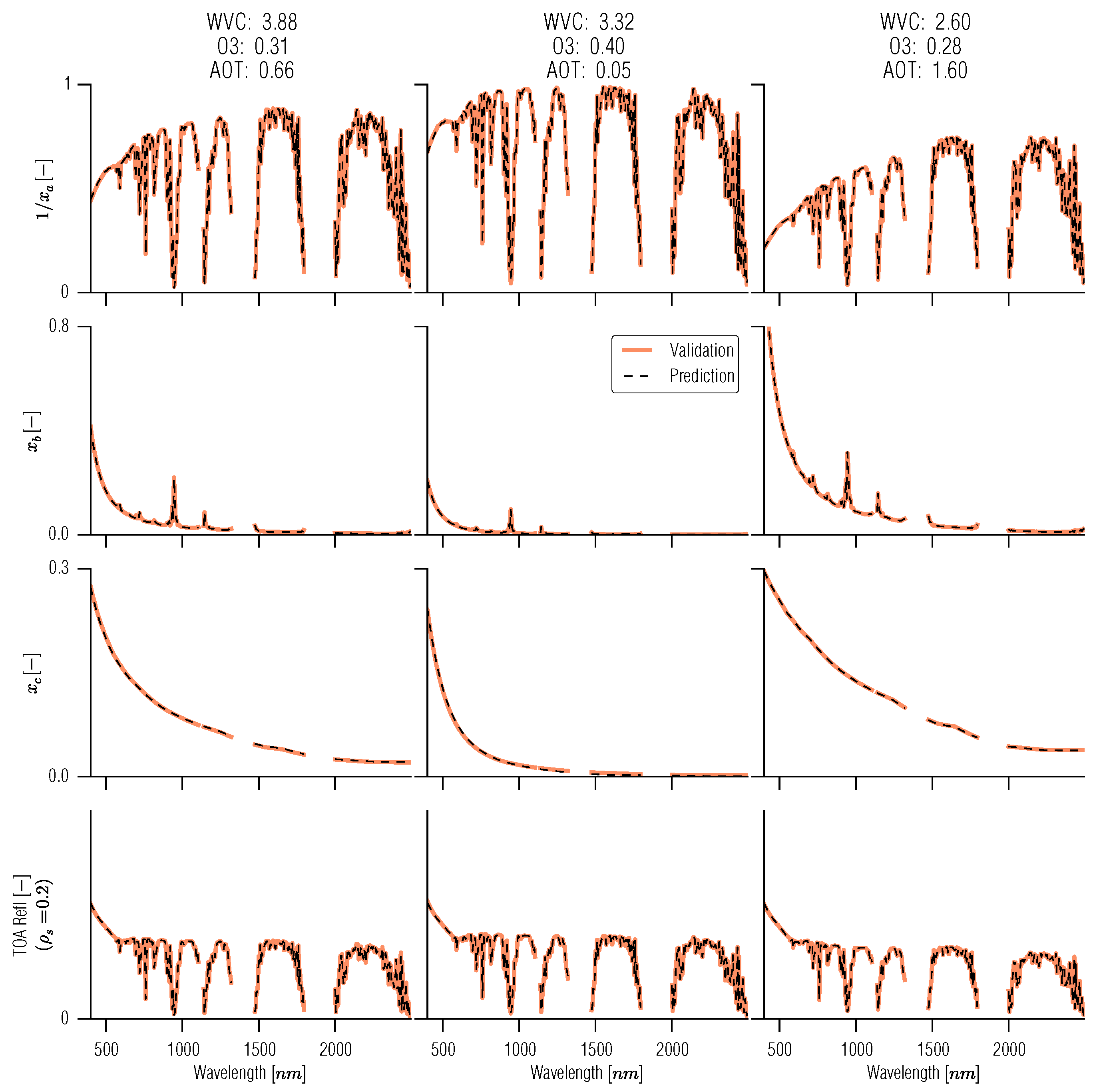
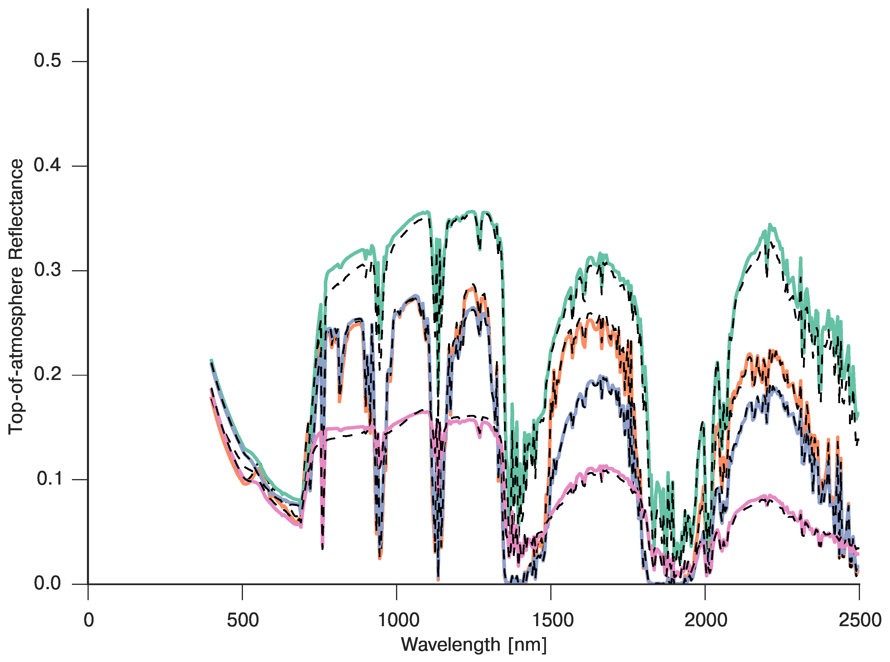
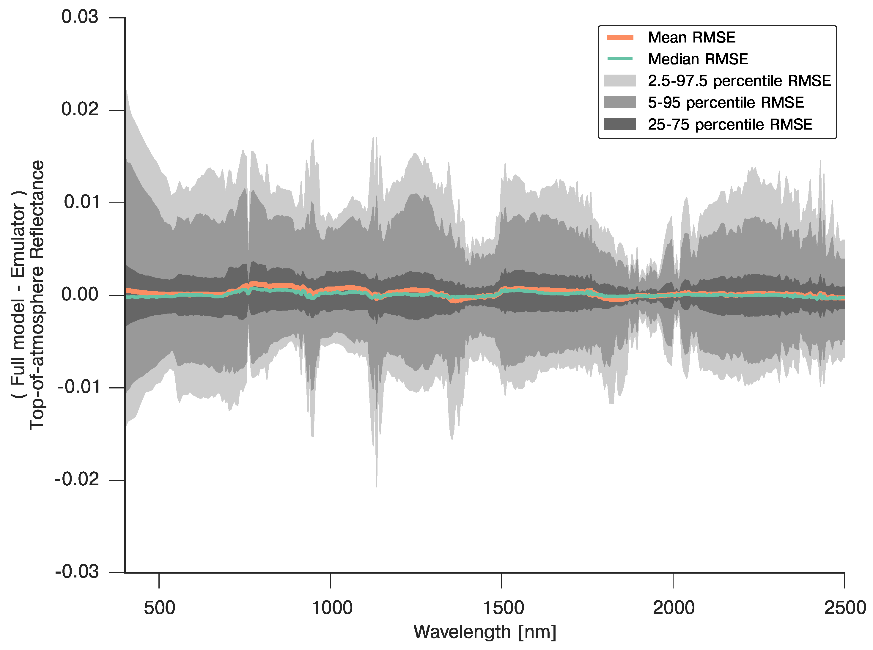
3.5. Full BRDF Coupling of a Soil-Leaf-Canopy Model and Atmospheric Spectral RT Model


4. Examples of the Use of GPs in Inverse Problems in Remote Sensing
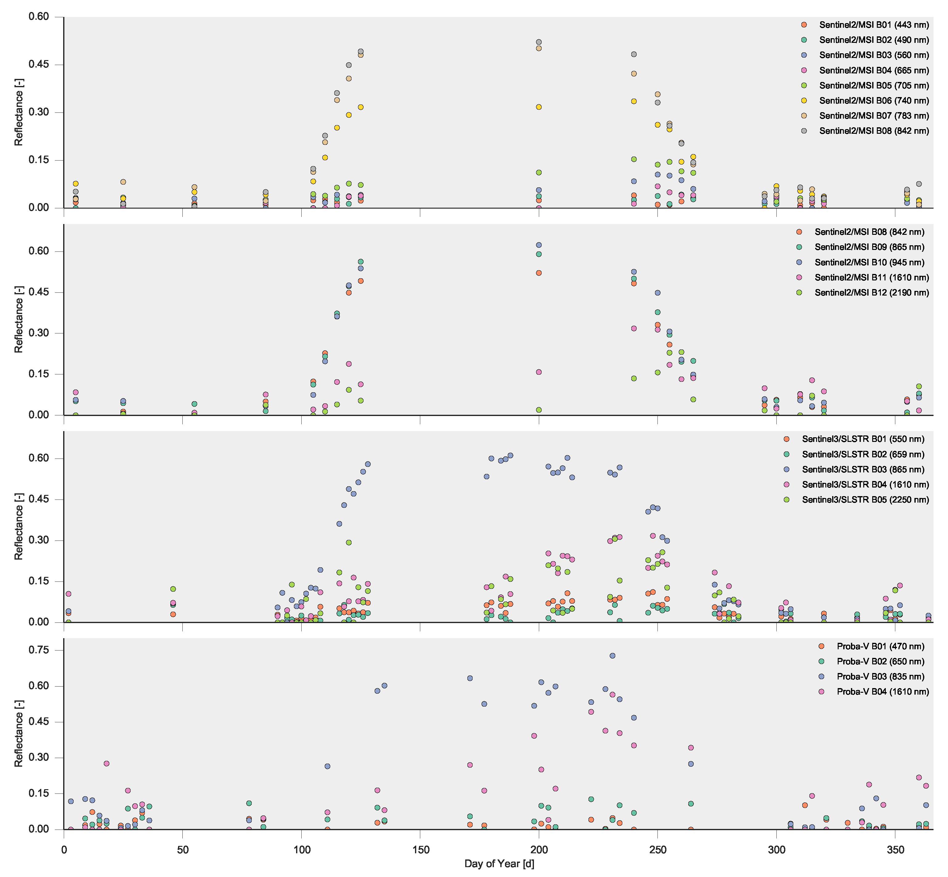
4.1. The Synthetic “Satellite” Observations
| Parameter | Value | ||||||
|---|---|---|---|---|---|---|---|
| N | 2.1 | – | – | – | – | – | – |
| 60 | 5 | 55 | -0.3 | 122 | 0.1 | 240 | |
| 7 | – | – | – | – | – | – | |
| 0.5 | – | – | – | – | – | – | |
| 0.0176 | 0.004 | 0.043 | −0.31 | 121 | 0.07 | 235 | |
| 0.002 | – | – | – | – | – | – | |
| 2 | 0.1 | 5 | −0.29 | 120 | 0.1 | 240 | |
| 70 | – | – | – | – | – | – | |
| 1.0 | – | – | – | – | – | – | |
| 0.3 | – | – | – | – | – | – |

| Parameter | Sentinel2/MSI | Sentinel3/SLSTR | Proba-V |
|---|---|---|---|
| Number of bands | 12 | 5 | 4 |
| Revisit frequency | 5 days | 2 days | 2 days |
| Overpass time | 10:30 AM | 10:00 AM | 11:00 AM |
| Variation in viewing zenith angle (VZA) | |||
| Percentage valid observations | 30% | 30% | 30% |
| Average temporal window | 12 days | 10 days | 11 days |
| Noise model slope m | 0.0042 | 0.0075 | 0.108 |
| Noise model intercept c | 0.0028 | 0.005 | 0.007 |
4.2. Generic Strategy for the Inverse Problem
Solving for the Posterior
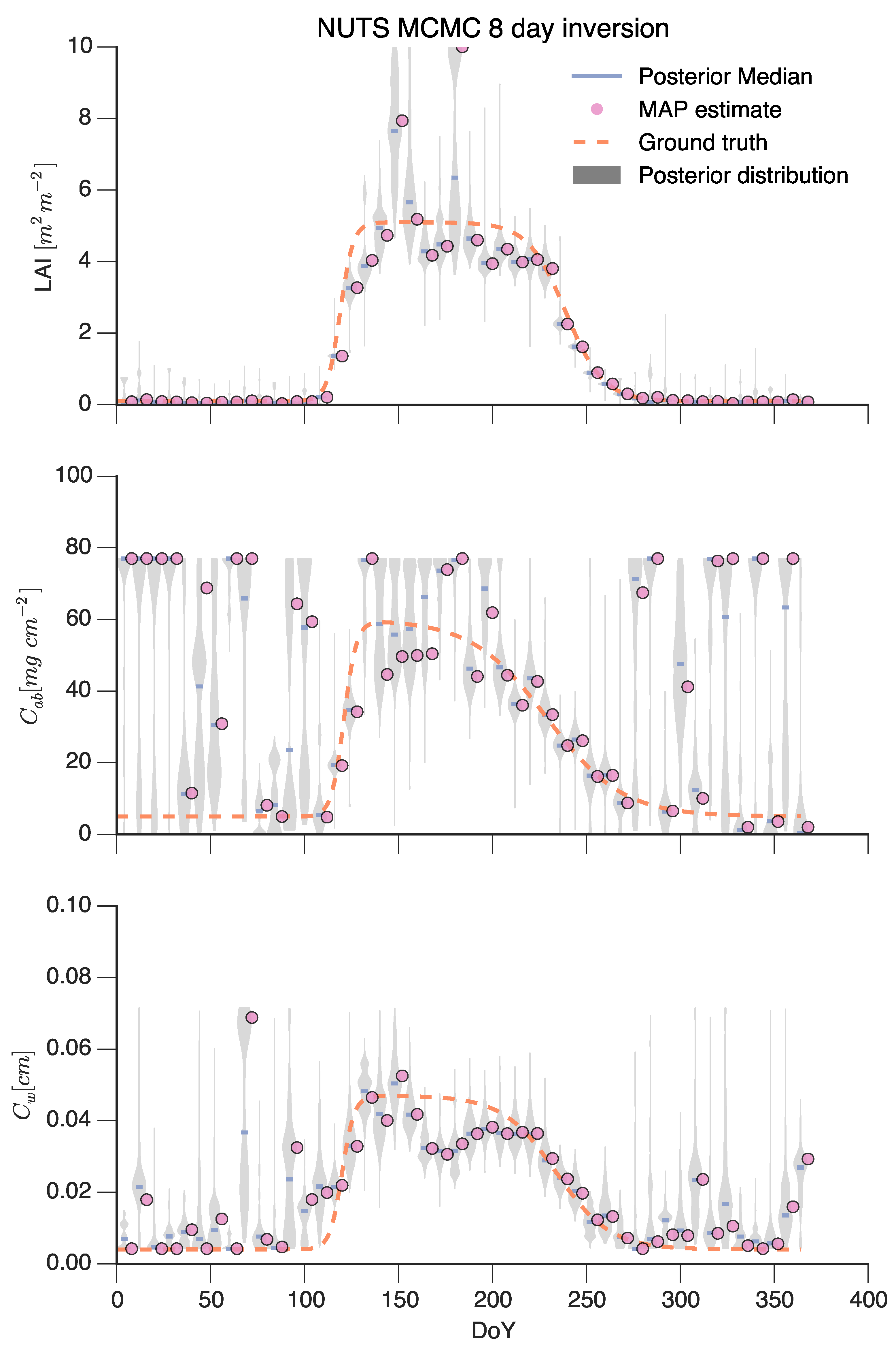
4.3. Inversion Using Markov Chain Monte Carlo (MCMC)
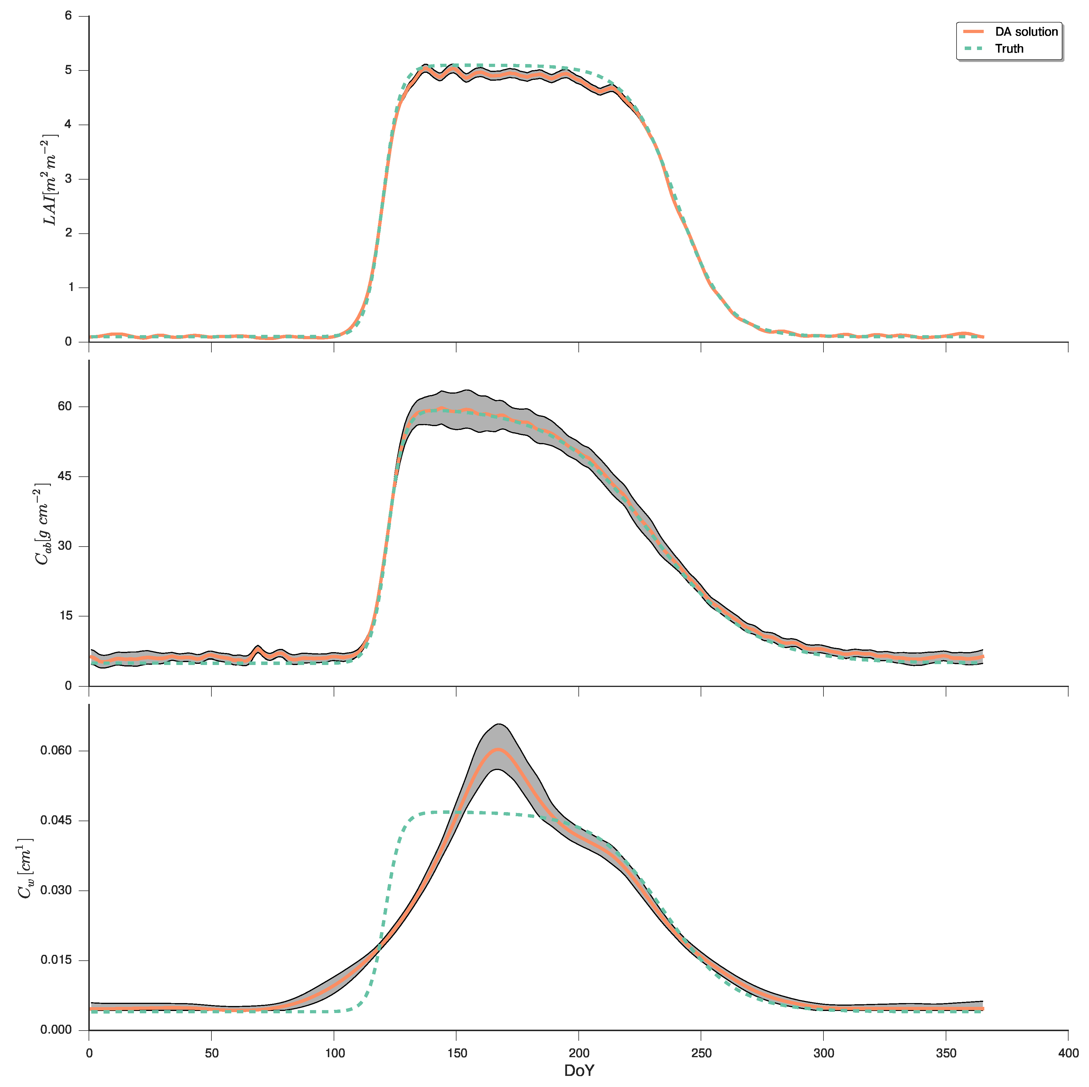
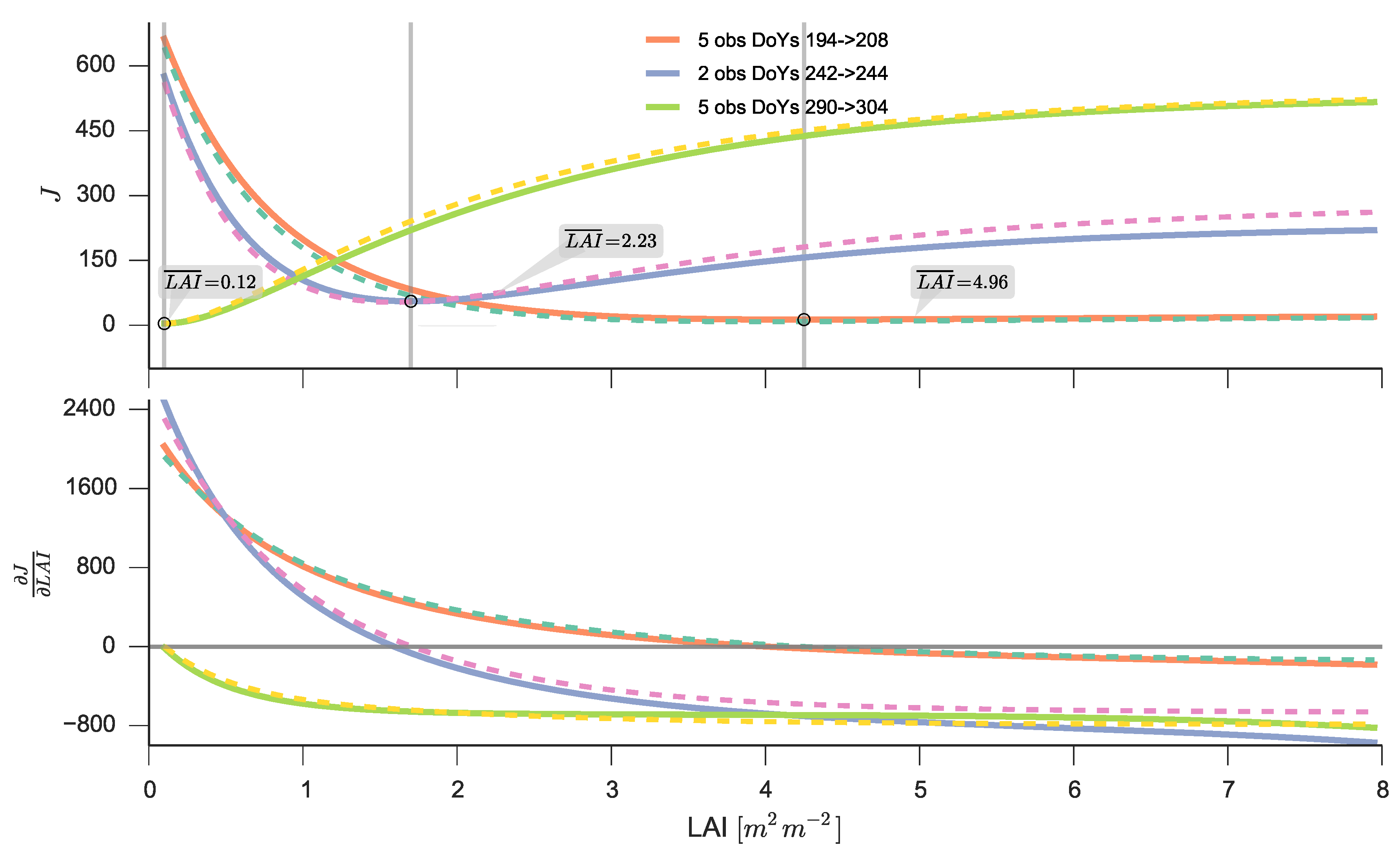
4.4. Variational DA Solution: EO-LDAS Framework

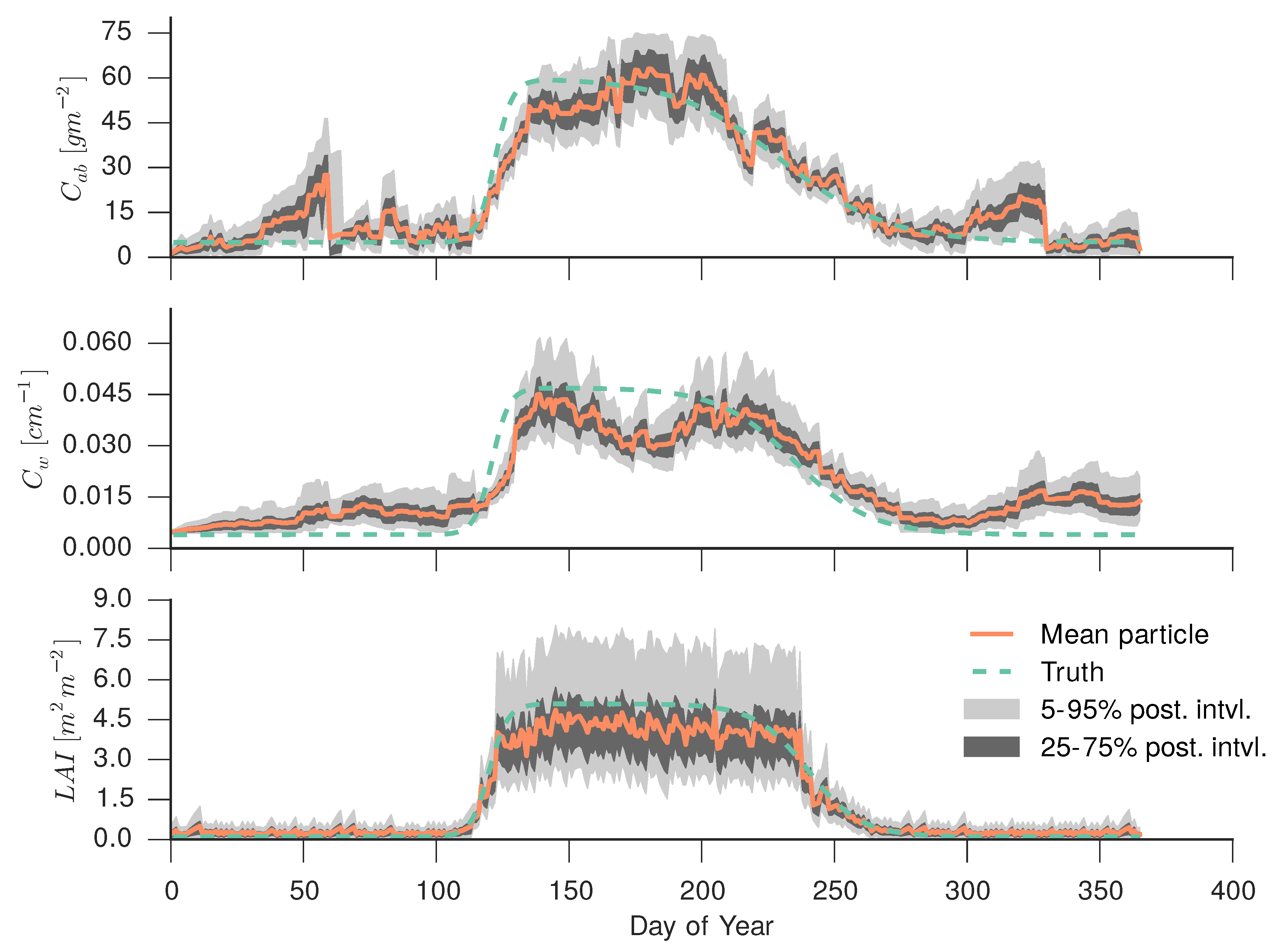
4.5. Simple Particle Filter
5. Discussion and Outlook
6. Conclusions
Acknowledgments
Author Contributions
Conflicts of Interest
References
- Wulder, M.A.; Hilker, T.; White, J.C.; Coops, N.C.; Masek, J.G.; Pflugmacher, D.; Crevier, Y. Virtual constellations for global terrestrial monitoring. Remote Sens. Environ. 2015, 170, 62–76. [Google Scholar] [CrossRef]
- Tarantola, A. Inverse Problem Theory and Methods for Model Parameter Estimation; SIAM: Philadelphia, PA, USA, 2005. [Google Scholar]
- Rodgers, C.D. Others. In Inverse Methods for Atmospheric Sounding: Theory and Practice; World Scientific: Singapore, 2000; Volume 2. [Google Scholar]
- Combal, B.; Baret, F.; Weiss, M.; Trubuil, A.; Mace, D.; Pragnere, A.; Myneni, R.; Knyazikhin, Y.; Wang, L. Retrieval of canopy biophysical variables from bidirectional reflectance: Using prior information to solve the ill-posed inverse problem. Remote Sens. Environ. 2003, 84, 1–15. [Google Scholar] [CrossRef]
- Yuan, H.; Dai, Y.; Xiao, Z.; Ji, D.; Shangguan, W. Reprocessing the MODIS Leaf Area Index products for land surface and climate modelling. Remote Sens. Environ. 2011, 115, 1171–1187. [Google Scholar] [CrossRef]
- Pinty, B.; Andredakis, I.; Clerici, M.; Kaminski, T.; Taberner, M.; Verstraete, M.M.; Gobron, N.; Plummer, S.; Widlowski, J.L. Exploiting the MODIS albedos with the Two-stream Inversion Package (JRC-TIP): 1. Effective leaf area index, vegetation, and soil properties. J. Geophys. Res. 2011, 116, D09105. [Google Scholar] [CrossRef]
- Lewis, P.; Gómez-Dans, J.; Kaminski, T.; Settle, J.; Quaife, T.; Gobron, N.; Styles, J.; Berger, M. An earth observation land data assimilation system (EO-LDAS). Remote Sens. Environ. 2012, 120, 219–235. [Google Scholar] [CrossRef]
- Giering, R.; Kaminski, T. Recipes for adjoint code construction. ACM Trans. Math. Softw. 1998, 24, 437–474. [Google Scholar] [CrossRef]
- Laurent, V.C.E.; Verhoef, W.; Clevers, J.G.P.W.; Schaepman, M.E. Estimating forest variables from top-of-atmosphere radiance satellite measurements using coupled radiative transfer models. Remote Sens. Environ. 2011, 115, 1043–1052. [Google Scholar] [CrossRef]
- Knyazikhin, Y.; Martonchik, J.V.; Myneni, R.B.; Diner, D.J.; Running, S.W. Synergistic algorithm for estimating vegetation canopy leaf area index and fraction of absorbed photosynthetically active radiation from MODIS and MISR data. J. Geophys. Res. 1998, 103, 32257–32275. [Google Scholar] [CrossRef]
- Kimes, D.S.; Nelson, R.F.; Manry, M.T.; Fung, A.K. Review article: Attributes of neural networks for extracting continuous vegetation variables from optical and radar measurements. Int. J. Remote Sens. 1998, 19, 2639–2663. [Google Scholar] [CrossRef]
- Baret, F.; Hagolle, O.; Geiger, B.; Bicheron, P.; Miras, B.; Huc, M.; Berthelot, B.; Niño, F.; Weiss, M.; Samain, O.; et al. LAI, fAPAR and fCover CYCLOPES global products derived from VEGETATION: Part 1: Principles of the algorithm. Remote Sens. Environ. 2007, 110, 275–286. [Google Scholar] [CrossRef] [Green Version]
- Verrelst, J.; Muñoz, J.; Alonso, L.; Delegido, J.; Rivera, J.P.; Camps-Valls, G.; Moreno, J. Machine learning regression algorithms for biophysical parameter retrieval: Opportunities for Sentinel-2 and -3. Remote Sens. Environ. 2012, 118, 127–139. [Google Scholar] [CrossRef]
- Verrelst, J.; Camps-Valls, G.; Muñoz Marí, J.; Rivera, J.P.; Veroustraete, F.; Clevers, J.G.P.W.; Moreno, J. Optical remote sensing and the retrieval of terrestrial vegetation bio-geophysical properties—A review. ISPRS J. Photogramm. Remote Sens. 2015, 108, 273–290. [Google Scholar] [CrossRef]
- Quaife, T.; Lewis, P.; De Kauwe, M.; Williams, M.; Law, B.E.; Disney, M.; Bowyer, P. Assimilating canopy reflectance data into an ecosystem model with an Ensemble Kalman Filter. Remote Sens. Environ. 2008, 112, 1347–1364. [Google Scholar] [CrossRef]
- Peng, C.; Guiot, J.; Wu, H.; Jiang, H.; Luo, Y. Integrating models with data in ecology and palaeoecology: advances towards a model–data fusion approach. Ecol. Lett. 2011, 14, 522–536. [Google Scholar] [CrossRef] [PubMed]
- Luo, Y.; Ogle, K.; Tucker, C.; Fei, S.; Gao, C.; LaDeau, S.; Clark, J.S.; Schimel, D.S. Ecological forecasting and data assimilation in a data-rich era. Ecol. Appl. 2011, 21, 1429–1442. [Google Scholar] [CrossRef] [PubMed]
- O’Hagan, A.; Kingman, J.F.C. Curve Fitting and Optimal Design for Prediction. J. R. Stat. Soc. Series B Stat. Methodol. 1978, 40, 1–42. [Google Scholar]
- Sacks, J.; Welch, W.J.; Mitchell, T.J.; Wynn, H.P. Design and analysis of computer experiments. Stat. Sci. 1989, 4, 409–423. [Google Scholar] [CrossRef]
- O’Hagan, A. Some Bayesian numerical analysis. Bayesian Stat. 1992, 4, 345–363. [Google Scholar]
- Kennedy, M.C.; O’Hagan, A. Predicting the output from a complex computer code when fast approximations are available. Biometrika 2000, 87, 1–13. [Google Scholar] [CrossRef]
- Challenor, P.G.; Hankin, R.K.S.; Marsh, R. Towards the probability of rapid climate change. In Avoiding Dangerous Climate Change; Cambridge University Press: Cambridge, UK, 2006; pp. 55–63. [Google Scholar]
- Rougier, J.; Sexton, D.M.H.; Murphy, J.M.; Stainforth, D. Analyzing the Climate Sensitivity of the HadSM3 Climate Model Using Ensembles from Different but Related Experiments. J. Climate 2009, 22, 3540–3557. [Google Scholar] [CrossRef] [Green Version]
- Picard, G.; Woodward, F.I.; Lomas, M.R.; Pellenq, J.; Quegan, S.; Kennedy, M. Constraining the Sheffield dynamic global vegetation model using stream-flow measurements in the United Kingdom. Glob. Chang. Biol. 2005, 11, 2196–2210. [Google Scholar] [CrossRef]
- Kennedy, M.; Anderson, C.; O’Hagan, A.; Lomas, M.; Woodward, I.; Gosling, J.P.; Heinemeyer, A. Quantifying uncertainty in the biospheric carbon flux for England and Wales. J. R. Stat. Soc. Ser. A 2008, 171, 109–135. [Google Scholar] [CrossRef]
- Morris, R.D.; Kottas, A.; Taddy, M.; Furfaro, R.; Ganapol, B.D. A statistical framework for the sensitivity analysis of radiative transfer models. IEEE Trans. Geosci. Remote Sens. 2008, 46, 4062–4074. [Google Scholar] [CrossRef]
- Pasolli, L.; Melgani, F.; Blanzieri, E. Gaussian process regression for estimating chlorophyll concentration in subsurface waters from remote sensing data. IEEE Geosci. Remote Sens. Lett. 2010, 7, 464–468. [Google Scholar] [CrossRef]
- Verrelst, J.; Alonso, L.; Camps-Valls, G.; Delegido, J.; Moreno, J. Retrieval of vegetation biophysical parameters using Gaussian process techniques. IEEE Trans. Geosci. Remote Sens. 2012, 50, 1832–1843. [Google Scholar] [CrossRef]
- Rivera Caicedo, J.P.; Verrelst, J.; Munoz-Mari, J.; Moreno, J.; Camps-Valls, G. Toward a semiautomatic machine learning retrieval of biophysical parameters. IEEE J. Sel. Top. Appl. Earth Observ. Remote Sens. 2014, 7, 1249–1259. [Google Scholar] [CrossRef]
- Simpson, T.W.; Poplinski, J.; Koch, P.N.; Allen, J.K. Metamodels for computer-based engineering design: survey and recommendations. Eng. Comput. 2001, 17, 129–150. [Google Scholar] [CrossRef]
- Wang, G.G.; Shan, S. Review of metamodeling techniques in support of engineering design optimization. J. Mech. Des. 2007, 129, 370–380. [Google Scholar] [CrossRef]
- Rasmussen, C.E.; Williams, C.K.I. Gaussian Processes for Machine Learning; The MIT Press: Cambridge, MA, USA, 2006. [Google Scholar]
- MacKay, D.J.C. Gaussian Processes—A Replacement for Supervised Neural Networks? 1997. Available online: http://www.inference.eng.cam.ac.uk/mackay/gp.pdf (accessed on 28 January 2016).
- Verhoef, W. Light scattering by leaf layers with application to canopy reflectance modeling: The SAIL model. Remote Sens. Environ. 1984, 16, 125–141. [Google Scholar] [CrossRef]
- Gobron, N.; Pinty, B.; Verstraete, M.M.; Govaerts, Y. A semidiscrete model for the scattering of light by vegetation. J. Geophys. Res. 1997, 102, 9431–9446. [Google Scholar] [CrossRef]
- Feret, J.B.; François, C.; Asner, G.P.; Gitelson, A.A.; Martin, R.E.; Bidel, L.P.R.; Ustin, S.L.; le Maire, G.; Jacquemoud, S. PROSPECT-4 and 5: Advances in the leaf optical properties model separating photosynthetic pigments. Remote Sens. Environ. 2008, 112, 3030–3043. [Google Scholar] [CrossRef]
- Jacquemoud, S.; Verhoef, W.; Baret, F.; Bacour, C.; Zarco-Tejadae, P.J.; Asnerf, G.P.; Françoisg, C.; Ustin, S.L. PROSPECT+ SAIL models: A review of use for vegetation characterization. Remote Sens. Environ. 2009, 13, 56–66. [Google Scholar] [CrossRef]
- Ju, J.; Roy, D.P.; Vermote, E.; Masek, J.; Kovalskyy, V. Continental-scale validation of MODIS-based and LEDAPS Landsat ETM+ atmospheric correction methods. Remote Sens. Environ. 2012, 122, 175–184. [Google Scholar] [CrossRef]
- Vermote, E.F.; Tanre, D.; Deuze, J.L.; Herman, M.; Morcette, J.J. Second simulation of the satellite signal in the solar spectrum, 6S: An overview. IEEE Trans. Geosci. Remote Sens. 1997, 35, 675–686. [Google Scholar] [CrossRef]
- Tanre, D.; Herman, M.; Deschamps, P.; Leffe, A.D. Atmospheric modeling for space measurements of ground reflectances, including bidirectional properties. Appl. Opt. 1979, 18, 3587–3594. [Google Scholar] [CrossRef] [PubMed]
- Guanter, L.; Richter, R.; Kaufmann, H. On the application of the MODTRAN4 atmospheric radiative transfer code to optical remote sensing. Int. J. Remote Sens. 2009, 30, 1407–1424. [Google Scholar] [CrossRef]
- MODIS Moderate resolution image spectroradiometer. Available online: http://modis.gsfc.nasa.gov/about/specifications.php (accessed on 28 January 2016).
- Roy, D.P.; Jin, Y.; Lewis, P.E.; Justice, C.O. Prototyping a global algorithm for systematic fire-affected area mapping using MODIS time series data. Remote Sens. Environ. 2005, 97, 137–162. [Google Scholar] [CrossRef]
- Wanner, W.; Li, X.; Strahler, A. On the derivation of kernels for kernel-driven models of bidirectional reflectance. J. Geophys. Res. Atmos. 1995, 100, 21077–21089. [Google Scholar] [CrossRef]
- Zhang, X.; Friedl, M.A.; Schaaf, C.B.; Strahler, A.H.; Hodges, J.C.F.; Gao, F.; Reed, B.C.; Huete, A. Monitoring vegetation phenology using MODIS. Remote Sens. Environ. 2003, 84, 471–475. [Google Scholar] [CrossRef]
- Koetz, B.; Baret, F.; Poilvé, H.; Hill, J. Use of coupled canopy structure dynamic and radiative transfer models to estimate biophysical canopy characteristics. Remote Sens. Environ. 2005, 95, 115–124. [Google Scholar] [CrossRef]
- Drusch, M.; del Bello, U.; Carlier, S.; Colin, O.; Fernandeza, V.; Gasconb, F.; Hoerschb, B.; Isolaa, C.; Laberintia, P.; Martimorta, P.; et al. Sentinel-2: ESA’s optical high-resolution mission for GMES operational services. Remote Sens. Environ. 2012, 120, 25–36. [Google Scholar] [CrossRef]
- Donlon, C.; Berruti, B.; Buongiorno, A.; Ferreira, M.H.; Féménias, P.; Frerick, J.; Goryl, P.; Klein, U.; Laur, H.; Mavrocordatos, C.; et al. The global monitoring for environment and security (GMES) sentinel-3 mission. Remote Sens. Environ. 2012, 120, 37–57. [Google Scholar] [CrossRef]
- Dierckx, W.; Sterckx, S.; Benhadj, I.; Livens, S.; Duhoux, G.; Achteren, T.V.; Francois, M.; Mellab, K.; Saint, G. PROBA-V mission for global vegetation monitoring: Standard products and image quality. Int. J. Remote Sens. 2014, 35, 2589–2614. [Google Scholar] [CrossRef]
- Zupanski, D. A general weak constraint applicable to operational 4DVAR data assimilation systems. Mon. Weather Rev. 1997, 125, 2274–2292. [Google Scholar] [CrossRef]
- Quaife, T.; Lewis, P. Temporal constraints on linear BRDF model parameters. IEEE Trans. Geosci. Remote Sens. 2010, 48, 2445–2450. [Google Scholar] [CrossRef]
- Kalman, R.E. A new approach to linear filtering and prediction problems. J. Basic Eng. 1960, 82, 35–45. [Google Scholar] [CrossRef]
- Evensen, G. The ensemble kalman filter: Theoretical formulation and practical implementation. Ocean Dyn. 2003, 53, 343–367. [Google Scholar] [CrossRef]
- Corporation, T.A.S.; Gelb, A. Applied Optimal Estimation; The MIT Press: Cambridge, MA, USA, 1974. [Google Scholar]
- Ristic, B.; Arulampalam, S.; Gordon, N.J. Beyond the Kalman Filter: Particle Filters for Tracking Applications; Artech House: Norwood, MA, USA, 2004. [Google Scholar]
- Van Leeuwen, P.J. Particle filtering in geophysical systems. Mon. Weather Rev. 2009, 137, 4089–4114. [Google Scholar] [CrossRef]
- Kantas, N.; Doucet, A.; Singh, S.S.; Maciejowski, J.; Chopin, N. On particle methods for parameter estimation in State-Space models. Stat. Sci. 2015, 30, 328–351. [Google Scholar] [CrossRef]
- Dowd, M. A sequential Monte Carlo approach for marine ecological prediction. Environmetrics 2006, 17, 435–455. [Google Scholar] [CrossRef]
- Dowd, M. Bayesian statistical data assimilation for ecosystem models using Markov Chain Monte Carlo. J. Mar. Syst. 2007, 68, 439–456. [Google Scholar] [CrossRef]
- Yang, W.; Tan, B.; Huang, D.; Rautiainen, M.; Shabanov, N.V.; Wang, Y.; Privette, J.L.; Huemmrich, K.F.; Fensholt, R.; Sandholt, I.; et al. MODIS leaf area index products: From validation to algorithm improvement. IEEE Trans. Geosci. Remote Sens. 2006, 44, 1885–1898. [Google Scholar] [CrossRef]
- Homan, M.D.; Gelman, A. The No-U-turn Sampler: Adaptively setting path lengths in Hamiltonian Monte Carlo. J. Mach. Learn. Res. 2014, 15, 1593–1623. [Google Scholar]
- The eoldas_ng library. Available online: http://github.com/jgomezdans/eoldas_ng (accessed on 28 January 2016).
- Bastos, L.S.; O’Hagan, A. Diagnostics for Gaussian process emulators. Technometrics 2009, 51, 425–438. [Google Scholar] [CrossRef]
- Xiao, Z.; Liang, S.; Wang, J.; Xie, D.; Song, J.; Fensholt, R. A framework for consistent estimation of Leaf Area Index, fraction of absorbed photosynthetically active radiation, and surface albedo from MODIS Time-Series data. IEEE Trans. Geosci. Remote Sens. 2015, 53, 3178–3197. [Google Scholar] [CrossRef]
- Gelfand, A.E.; Schmidt, A.M.; Banerjee, S.; Sirmans, C.F. Nonstationary multivariate process modeling through spatially varying coregionalization. Test 2004, 13, 263–312. [Google Scholar] [CrossRef]
- Paciorek, C.J.; Schervish, M.J. Nonstationary covariance functions for Gaussian process regression. In Advances in Neural Information Processing Systems 16; Thrun, S., Saul, L.K., Schölkopf, B., Eds.; MIT Press: Cambridge, MA, USA, 2004; pp. 273–280. [Google Scholar]
- Lauvernet, C.; Baret, F.; Hascoët, L.; Buis, S.; le Dimet, F.X. Multitemporal-patch ensemble inversion of coupled surface–atmosphere radiative transfer models for land surface characterization. Remote Sens. Environ. 2008, 112, 851–861. [Google Scholar] [CrossRef]
- Laurent, V.C.E.; Verhoef, W.; Clevers, J.G.P.W.; Schaepman, M.E. Inversion of a coupled canopy–atmosphere model using multi-angular top-of-atmosphere radiance data: A forest case study. Remote Sens. Environ. 2011, 115, 2603–2612. [Google Scholar] [CrossRef]
- Mousivand, A.; Menenti, M.; Gorte, B.; Verhoef, W. Multi-temporal, multi-sensor retrieval of terrestrial vegetation properties from spectral–directional radiometric data. Remote Sens. Environ. 2015, 158, 311–330. [Google Scholar] [CrossRef]
- Ma, G.; Huang, J.; Wu, W.; Fan, J.; Zou, J.; Wu, S. Assimilation of MODIS-LAI into the WOFOST model for forecasting regional winter wheat yield. Math. Comput. Model. 2013, 58, 634–643. [Google Scholar] [CrossRef]
- Conti, S.; Gosling, J.P.; Oakley, J.E.; O’Hagan, A. Gaussian process emulation of dynamic computer codes. Biometrika 2009. [Google Scholar] [CrossRef]
- Rougier, J. Efficient emulators for multivariate deterministic functions. J. Comput. Graph. Stat. 2008, 17, 827–843. [Google Scholar] [CrossRef]
- Loew, A.; van Bodegom, P.M.; Widlowski, J.L.; Otto, J.; Quaife, T.; Pinty, B.; Raddatz, T. Do we (need to) care about canopy radiation schemes in DGVMs? Caveats and potential impacts. Biogeosciences 2014, 11, 1873–1897. [Google Scholar] [CrossRef]
- Higdon, D.; Swall, J.; Kern, J. Non-stationary spatial modeling. Bayesian Stat. 1999, 6, 761–768. [Google Scholar]
- Efremenko, D.S.; Loyola, D.G.; Doicu, A.; Spurr, R.J. Multi-core-CPU and GPU-accelerated radiative transfer models based on the discrete ordinate method. Comput. Phys. Commun. 2014, 185, 3079–3089. [Google Scholar] [CrossRef]
- Gomez-Dans, J.L.; Lewis, P.E. Python code for Gaussian process emulation of radiative transfer models. Available online: http://jgomezdans.github.io/gp_emulator (accessed on 28 January 2016). [CrossRef]
- Wilson, R. Py6S: A Python interface to the 6S radiative transfer model. Comput. Geosci. 2013, 51, 166–171. [Google Scholar] [CrossRef]
© 2016 by the authors; licensee MDPI, Basel, Switzerland. This article is an open access article distributed under the terms and conditions of the Creative Commons by Attribution (CC-BY) license (http://creativecommons.org/licenses/by/4.0/).
Share and Cite
Gómez-Dans, J.L.; Lewis, P.E.; Disney, M. Efficient Emulation of Radiative Transfer Codes Using Gaussian Processes and Application to Land Surface Parameter Inferences. Remote Sens. 2016, 8, 119. https://doi.org/10.3390/rs8020119
Gómez-Dans JL, Lewis PE, Disney M. Efficient Emulation of Radiative Transfer Codes Using Gaussian Processes and Application to Land Surface Parameter Inferences. Remote Sensing. 2016; 8(2):119. https://doi.org/10.3390/rs8020119
Chicago/Turabian StyleGómez-Dans, José Luis, Philip Edward Lewis, and Mathias Disney. 2016. "Efficient Emulation of Radiative Transfer Codes Using Gaussian Processes and Application to Land Surface Parameter Inferences" Remote Sensing 8, no. 2: 119. https://doi.org/10.3390/rs8020119