Article

Estimation of Winter Wheat Biomass and Yield by Combining the AquaCrop Model and Field Hyperspectral Data

1
Key Laboratory of Wetland Ecology and Environment, Northeast Institute of Geography and Agroecology, Chinese Academy of Sciences, Changchun 130102, China
2
Ecosystem Management, School of Environmental and Rural Science, University of New England, Armidale, NSW 2351, Australia
3
Beijing Research Center for Information Technology in Agriculture, Beijing Academy of Agriculture and Forestry Sciences, Beijing 100097, China
4
National Engineering Research Center for Information Technology in Agriculture, Beijing 100097, China
*
Author to whom correspondence should be addressed.
Remote Sens. 2016, 8(12), 972; https://doi.org/10.3390/rs8120972
Submission received: 9 August 2016 / Revised: 16 November 2016 / Accepted: 18 November 2016 / Published: 24 November 2016
(This article belongs to the Special Issue Remote Sensing of Above Ground Biomass)

Abstract

:
Knowledge of spatial and temporal variations in crop growth is important for crop management and stable crop production for the food security of a country. A combination of crop growth models and remote sensing data is a useful method for monitoring crop growth status and estimating crop yield. The objective of this study was to use spectral-based biomass values generated from spectral indices to calibrate the AquaCrop model using the particle swarm optimization (PSO) algorithm to improve biomass and yield estimations. Spectral reflectance and concurrent biomass and yield were measured at the Xiaotangshan experimental site in Beijing, China, during four winter wheat-growing seasons. The results showed that all of the measured spectral indices were correlated with biomass to varying degrees. The normalized difference matter index (NDMI) was the best spectral index for estimating biomass, with the coefficient of determination (R2), root mean square error (RMSE), and relative RMSE (RRMSE) values of 0.77, 1.80 ton/ha, and 25.75%, respectively. The data assimilation method (R2 = 0.83, RMSE = 1.65 ton/ha, and RRMSE = 23.60%) achieved the most accurate biomass estimations compared with the spectral index method. The estimated yield was in good agreement with the measured yield (R2 = 0.82, RMSE = 0.55 ton/ha, and RRMSE = 8.77%). This study offers a new method for agricultural resource management through consistent assessments of winter wheat biomass and yield based on the AquaCrop model and remote sensing data.

1. Introduction

Wheat is an important food source for the rapidly increasing population in China [1]. The attention paid to national food security and sustainable agricultural development has increased over recent years, with increased concern for the improvement of field wheat management. Therefore, it is important to estimate wheat growth status and predict wheat yield in a timely and accurate way [2]. The integration of crop models and remote sensing data has become a useful method for monitoring crop growth status and crop yield based on data assimilation over extensive regions [3,4].
In most cases, researches have developed remote sensing and crop models used in their respective study areas [5]. Crop models simulate crop physiological growth status using mathematical formulas [6]. They have been used to analyze the influences of climate, soil conditions, and management strategies on agronomic parameters (e.g., canopy aboveground biomass, LAI, and grain yield) [7]. The Agricultural Model Intercomparison and Improvement Project (AgMIP) recently reviewed 27 wheat models from around the world [8]. This review showed that poor performance may be obtained when a crop model is applied over a large region due to uncertainties in the spatial distribution of soil properties, initial model conditions, crop parameters, and field management practices, resulting in biased simulations [9,10]. Large amounts of high-quality data have been used to improve the calibration and parameterization of crop models, thereby increasing the simulation accuracy of crop models on a regional scale.
Rapid development of remote sensing technology has facilitated the acquisition of crop growth information with high temporal and spatial resolutions [5,11,12,13,14,15,16]. Previous studies have indicated that combining crop models and remote sensing data can be used to improve the accuracy of crop yield estimates [17,18,19,20,21,22,23,24,25]. Curnel et al. [17] evaluated the feasibility of assimilating wheat leaf area index (LAI) derived from remote sensing data into the World Food Studies’ (WOFOST) crop growth model using a recalibration-based assimilation method; the results indicated that remote sensing data can be used to improve yield estimations. Dente et al. [19] assimilated LAI from Environment Satellite (ENVISAT) Advanced Synthetic Aperture Radar (ASAR) and Medium Resolution Imaging Spectrometer (MERIS) data into the Crop Estimation through Resource and Environment Synthesis-Wheat (CERES-Wheat) model at a catchment scale using a variational assimilation algorithm; the results suggested that this approach minimizes the difference between simulated and remotely-sensed LAI and achieves high estimation accuracy. Soil moisture data from the Advanced Microwave Scanning Radiometer-EOS (AMSR-E) and LAI from the Moderate Resolution Imaging Spectroradiometer-LAI (MODIS-LAI) were assimilated into the Decision Support System for Agro-technology Transfer-Cropping System Model (DSSAT-CSM)-Maize using an Ensemble Kalman Filter algorithm, and simulated yield was more accurate when both LAI and soil moisture were used [22]. The ensemble-based four-dimensional variational method was used to assimilate HJ-1A/B satellite data into the CERES-Wheat model, and estimates of winter wheat yield in field plots were reported (R2 = 0.73; RMSE = 319 kg/ha) [23]. Huang et al. [25] assimilated time series of LAI data with a 30-m spatial resolution into the WOFOST model with a Kalman Filter (KF) algorithm and reported more accurate estimates of regional winter wheat yield compared with more traditional approaches.
The integration of crop models and remotely sensed data using optimization algorithms (data assimilation methods) is becoming an effective and potential method for monitoring crop growth status and estimating crop yields, as it overcomes certain defects and combines the advantages of individual methods [5,26,27,28,29,30]. The data assimilation method can be used to reduce uncertainty in crop models to ensure that the simulated state variables (e.g., LAI and biomass) are in agreement with the measured state variables from remote sensing data. Several assimilation schemes have been developed [3,12,31,32,33]. Delecolle et al. [34] divided schemes into three categories. The first is the forcing method, in which state variables in crop models are directly substituted by remote sensing variables. This method is easy to use, but it relies on the calibrated parameters of crop models and the accuracy of remote sensing data [5,12]. The second is the calibration method, in which the initial parameters of crop models are recalibrated, based on the relationship between the remote sensing state variables and the simulated state variables [5,10,34]. In recent years, the calibration method has gained more attention, as it has greatly benefited from several intelligent optimization algorithms. The main shortcoming of the calibration method is that a great deal of computation time is required [3,5,30]. The third is the updating method, in which the simulated state variables are continuously renewed whenever remote sensing state variables are available. It is more flexible than the forcing method, but the remote sensing data must be of a higher accuracy than those of the simulated state variables, and this method heavily relies on the selection of the remote sensing data [4,33,35].
The combination of remote sensing data and light-driven or carbon-driven models has been widely studied, but few studies have focused on water-driven models for estimating the biomass and yield of crops. Therefore, in this study we focused on the AquaCrop model, a water-driven crop model, which was recently introduced to optimize crop water management strategies and improve crop yield in irrigation regions [36]. Winter wheat is the main crop grown in the North China Plain (NCP), and thus an important food source in China. Increased industrial and domestic water use has resulted in reduced water availability for irrigation of winter wheat crops. Therefore, improving water resource management in this region is crucial for increasing winter wheat yield. The main goal of this study was to improve estimates of winter wheat biomass and yield by assimilating field spectroscopic data into the AquaCrop model with a Particle Swarm Optimization (PSO) algorithm. The biomass and yield of winter wheat were used to optimize field irrigation management strategies and then to increase water use efficiency under different planting dates and irrigation management strategies. The specific objectives of this study were: (1) to select the best spectral indices from hyperspectral data for estimating winter wheat biomass; (2) to calibrate the AquaCrop model with biomass estimates derived from these indices using the PSO algorithm for improving accuracy of biomass and yield estimates; and (3) to evaluate the performance of the data assimilation method in estimating wheat biomass and yield.

2. Methodology

2.1. Description of the Study Site

Field experiments were carried out during the 2008/2009, 2009/2010, 2010/2011, and 2011/2012 growing seasons, at the Xiaotangshan experimental site (40°10′31″~40°11′18″N, 116°26′10″~116°27′05″E), Beijing, PR China. The soil type in the study site is fine-loamy. Beijing is characterized by a typical continental climate. The maximum temperature is 26.1 °C in summer, and the minimum temperature is −4.7 °C in winter. For the experimental period, the average annual precipitation was 650 mm and the frost-free period was 180 days on average [37].

2.2. Experimental Setup

Table 1 shows the winter wheat planting dates and cultivars. The area of each plot was 100 m2, in 2008, 2009, and 2010, and 300 m2 in 2011. A two-way factorial arrangement of treatments (winter wheat cultivar and planting date) in a randomized complete block design with three replicates was used in this experiment. Weed control, pest management, and fertilizer application were performed according to the local standard practices for wheat production.

2.3. Data Acquisition

2.3.1. Meteorological Data Collection

The local Xiaotangshan meteorological station was used to obtain meteorological data. Daily relative humidity, rainfall, total sunshine hours, wind speed, and maximum, minimum, and mean temperatures were recorded directly at the Xiaotangshan experimental site. The Food and Agriculture Organization Penman–Monteith method was used to calculate the reference evapotranspiration (ETo) [38].

2.3.2. Measurement of Canopy Reflectance

Spectral measurements of winter wheat were taken at different growth stages. The specific growth stages and dates are presented in Table 2. All canopy spectral measurements were taken at a nadir orientation, 1.0 m above the canopy, under clear sky condition between 10:00 and 14:00 Beijing local time, using an ASD Field Spec Pro Spectrometer (Analytical Spectral Devices, Boulder, CO, USA). The spectrometer was fitted with a 25° field of view optical fiber, operating in the 350–2500 nm spectral region. The scanned area of the ASD sensor was about 0.70 m2. A 40 × 40 cm BaSO4 calibration panel was used for calculating the black and baseline reflectance. Spectral measurements taken at all four sites in each plot were averaged to represent the canopy reflectance of each plot to reduce the possible effects due to field conditions. Vegetation radiance measurements were averaged from 10 scans at an optimized combination time at each site, and a dark current correction was conducted before each measurement. For each plot, a total of 40 spectra data points were obtained. Panel radiance measurements were taken twice, before and after the canopy spectral measurements.

2.3.3. Biomass and Yield Data Collection

The aboveground biomass, at the measuring positions of canopy spectral reflectance data, were obtained 5–6 times using random sampling of a 0.25-m2 area, in 2009–2012, with four replicates from each plot. A 4 × 0.25 m2 area for each plot was deemed sufficient, based on previous results [3]. All samples were heated to 105 °C, then oven dried at 70 °C to a constant weight, and their final dry weights were recorded.
The grain yields of each plot with three replicates for each treatment were obtained by randomly sampling a 1.5-m2 area. Finally, selected grain was dried and weighed on an electronic scale (±0.01 g).

2.3.4. Selection of Spectral Indices and Biomass Estimation from Spectral Indices

Fifteen spectral indices from the literature [13,16,39,40,41,42,43,44,45,46,47,48,49,50], determined to be good candidates for estimating biomass, were selected for the entire winter wheat growing season, based on 2009, 2010, and 2011 field data (Table 3). To refine the relationships between spectral indices and biomass, linear and nonlinear regression relationships between each of the spectral indices and biomass were determined based on field data from all growth stages during 2009, 2010, and 2011 (n = 135, calibration dataset). Field data taken in 2012 (n = 20, validation dataset) was used to validate the estimation accuracy of the models. Since the four winter wheat cultivars exhibited larger differences in 2012, resulting in greater variation in the biomass of the four winter wheat cultivars, the dataset from 2012 was selected to validate the estimation accuracy of the models. To determine the most sensitive spectral indices, we compared the coefficient of determination (R2), root mean square error (RMSE), and relative RMSE (RRMSE) values of the different models. Best-fitting regression equations were used for estimating winter wheat biomass. In addition, the homoscedasticity values (F) of the estimated and measured biomass were calculated using Levene’s test [51].

2.4. Description of the AquaCrop and ACsaV40 (AquaCrop Plug-In) Models

2.4.1. Description of the AquaCrop Model

The AquaCrop model was reported by the FAO in 2009, and detailed descriptions are reported in Steduto et al. [36], Raes et al. [52], and Jin et al. [37]. It computes daily crop transpiration and soil evaporation. The model subsequently estimates yield based on daily crop transpiration [36].

2.4.2. Description of the ACsaV40 (AquaCrop Plug-In) Model

The AquaCrop plug-in program, ACsaV40, was created to simultaneously run large amounts of data without a user interface [53]. It facilitates external and practical applications of AquaCrop. The input parameters of ACsaV40 are sorted in a text file, which can be created using the AquaCrop model, or by manually replacing the values of each variable with new values in the existing text files [54]. ACsaV40 runs the successive project files, and the simulated results of each project file are reserved in an output file, which includes the simulation period, stress factors, canopy cover, biomass, crop yield, and so on [53].

2.5. Assimilation of the AquaCrop Model and Remote Sensing Data Using the Particle Swarm Optimization (PSO) Algorithm

Particle swarm optimization (PSO) is a comparatively simple principle that can be easily combined into crop models with high calculation efficiency and few input parameters. Compared with various optimization algorithms, PSO is easier to apply in a practical study and has the advantages of a high precision and rapid convergence [55]. It has received widespread attention among scientists who have demonstrated its superiority in solving practical problems. In addition, PSO has the capability of parallel computing. Therefore, we used PSO to carry out the assimilation of remote sensing data into the AquaCrop model. PSO is based on the assumption of a group consisting of m (25 groups in this study) particles with certain speeds, without quality and size, in a d-dimensional search space. Each particle can modify its position and velocity based on both the best point in the current generation (pid) and the best point of all particles in the swarm (pgd). In this study, estimated biomass was used to optimize the crop parameters used in the AquaCrop model to obtain the optimal simulated biomass based on the fit of the cost function. The corresponding optimal yield is produced when the optimal simulated biomass is achieved. The PSO assimilation method for the The AquaCrop model and remote sensing data are presented in Figure 1. The specific steps to execute the PSO are as follows:
(1)
The velocity and position (initial value) of each particle are determined. The adjusted parameters include eight crop parameters (cgc, ccx, cdc, eme, num, psen, pstoshp, and rootdep) [56]. Specific information and ranges for these parameters are listed in Table 4.
(2)
ACsaV40 is executed with the required data using MATLAB (version 2007, MathWorks, Natick, MA, USA), and simulated biomass (BIOs) is obtained.
(3)
Regression relationships between spectral indices and measured biomass are analyzed, and the best regression model is determined to estimate biomass (BIOe).
(4)
A cost function is constructed according to the relationship BIOs and BIOe, reflecting the difference between BIOs and BIOe. The fit of the cost function determines whether the optimization algorithm had achieved the optimal input parameters.
(5)
The values of pid and pgd are searched in each iteration.
(6)
The position and velocity of each particle are updated based on pid and pgd. The values of C1 and C2 are set as 2, and random values between 0 and 1 are assigned to ξ and η [57].
(7)
If the iteration target (100 generations) is not reached, the updated positions are replaced and the previous step is repeated.
(8)
If the final iteration is achieved, the values of BIOs and corresponding simulated YIELDs are produced.

3. Results

3.1. Biomass Estimation

The regression relationships between biomass and spectral indices are provided in Table 5. The lowest and highest R2 values (0.25 and 0.84) were obtained for DCNI I and NDMI, respectively. The order of the spectral indices was WI I, WI II, NDII, NDMI, TBWI, EVI, TCARI, OSAVI, TCARI/OSAVI, MTCI, CIred edge, NDVI, DCNI I, OSAVI × CIred edge, and WDRVI. Of the R2 values, two were above 0.70, five were equal to or above 0.60, and eight were below 0.6. All spectral indices were fitted to power regression equations, with the exception of NDMI, DCNI I, and WDRVI, which were fitted to exponential regression equations (Table 5). The result showed that the assumption of homoscedasticity is met, based on the calculated F values between the estimated and measured biomass (Table 5).
The correlation between biomass and NDMI was highest compared with the other spectral indices, and the corresponding RMSE and RRMSE values for measured (BIOm) and estimated (BIOe) biomass were 1.80 ton/ha and 25.75%, respectively, which were lower than the values for the other indices (Table 5 and Figure 2). Therefore, NDMI was selected to estimate winter wheat biomass.

3.2. Data Assimilation for Biomass Estimation

The value of BIOe derived from the NDMI exponential regression equation was used as a variable to calibrate the AquaCrop model using the PSO algorithm. The results are presented in Figure 3 and Table 6, and the statistical regression equations are shown in Table 6. The BIOs was consistent with the BIOm across four years with different winter wheat cultivars, sowing dates, and irrigation management strategies, and the corresponding R2 and RMSE values were 0.83 and 1.65 ton/ha, respectively. The estimation accuracies of our experiments varied between years. The R2 and RMSE values were 0.81 and 1.69 ton/ha for 2008/2009, 0.82 and 1.67 ton/ha for 2009/2010, 0.81 and 1.56 ton/ha for 2010/2011, and 0.87 and 1.72 ton/ha for 2011/2012. The RRMSE values ranged from 23.60% to 30.65%. The deviation between the BIOs and BIOm in 2008/2009 was larger than that for the other years. Strong relationships between BIOs and BIOm were found, although biomass was often overestimated when the measured values exceeded 2 ton/ha (Figure 3). However, biomass was underestimated when the measured values were less than 2 ton/ha. The value of F was from 0.87 to 0.96 between the simulated and measured biomass (Table 6). The results show that the assumption of homoscedasticity was met.
We compared BIOs with BIOe using the spectral index method. The data assimilation method (R2 = 0.83 and RMSE = 1.65 ton/ha, Table 6) achieved better biomass estimations than the spectral index method (R2 = 0.77 and RMSE = 1.80 ton/ha, Table 5).

3.3. Data Assimilation for Yield

The yield of winter wheat was obtained after the data assimilation. The relationship between the measured and simulated yields is shown in Figure 4 and Table 7. There was a significant relationship between simulated (YIELDs) and measured (YIELDm) yield across all four years (R2 and RMSE values of 0.82 and 0.55 ton/ha, respectively) (Table 7). YIELDs varied between the four growing seasons. The R2 and RMSE values for YIELDs and YIELDm were 0.79 and 0.51 ton/ha in 2008/2009, 0.83 and 0.57 ton/ha in 2009/2010, 0.81 and 0.52 ton/ha in 2010/2011, and 0.89 and 0.61 ton/ha in 2011/2012, respectively. The value of RRMSE ranged from 8.77% to 10.69%. There was a wider range of YIELDs values in 2008/2011 than in 2011/2012 because of the different sowing treatments (Figure 4). A good relationship between YIELDs and YIELDm was also found. Yield was often overestimated when the YIELDm was higher than 5 ton/ha (Figure 4) and underestimated when the YIELDm was less than 5 ton/ha. Table 7 shows that the F values ranged from 0.72 to 0.87. The results demonstrated that the assumption of homoscedasticity was met.

4. Discussion

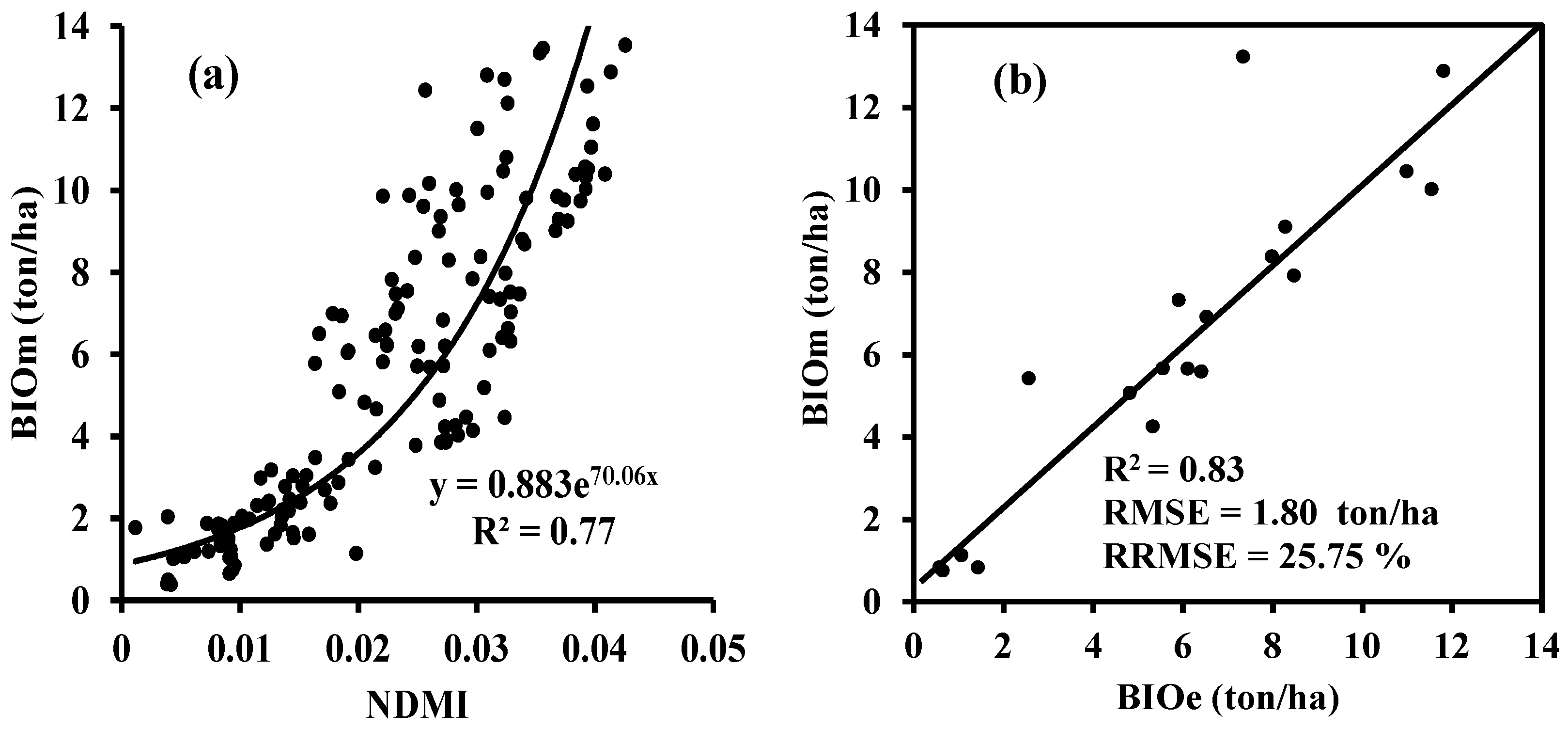
Spectral data and concurrent biomass and yield were acquired during four winter wheat growing seasons. Fifteen spectral indices were related to biomass (Table 5); this is because red edge (670–780 nm) and near infrared (short NIR, 800-1100 nm) data contain useful information regarding vegetation biomass [13,39,44,50]. In particular, NDMI was found to be highly correlated with biomass, with R2 and RMSE values of 0.77 and 1.80 ton/ha, respectively. NDMI does not contain red edge or short NIR data because absorption at these wavelengths is strongly influenced by chlorophyll content and canopy structure, which reduce the signal compared with that of dry matter. However, NDMI contains data at 1649 and 1722 nm, which are more sensitive to changes in dry matter [42]. These data were combined to establish NDMI, which includes signals from dry matter. For this reason, NDMI was more highly related with biomass than the other spectral indices and achieved more accurate biomass estimations. In this study, the linear and nonlinear regression relationships between each spectral index and biomass were analyzed to select the best-fitting regression equations. The results show that some models were fitted using power regression, and others fitted using exponential regression (Table 5). The difference between two regressions may have a close relationship with each spectral index and biomass dataset.
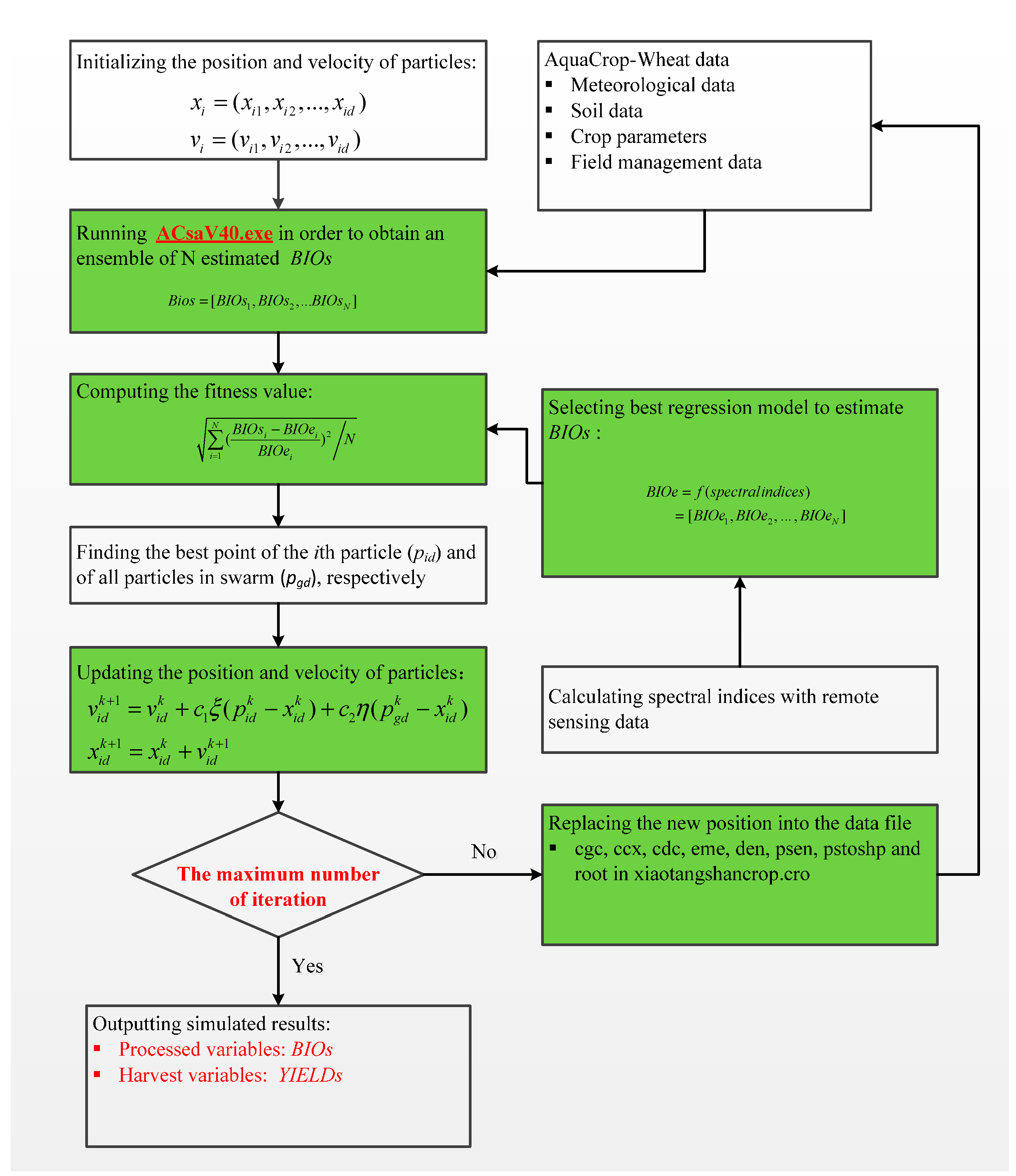
The model’s initial variables (num and eme) and crop parameters (cgc, ccx, cdc, eme, psen, and rootdep) were calibrated by combining biomass retrieved from spectral indices and the AquaCrop model via the PSO assimilation algorithm, thereby achieving optimal biomass estimations. The simulated biomass values were consistent with the measured values. These findings are consistent with those of Soddu et al. [58]. Heng et al. [59] showed that the AquaCrop model is used to better simulate biomass when irrigation is adequate. Our results suggest that the AquaCrop model could be used to simulate winter wheat biomass. The data assimilation method, based on the PSO algorithm, achieved better biomass estimations than the spectral index method (Table 5 and Table 6). The main reasons are as follows: (i) The AquaCrop model can be used to simulate dry biomass accumulation on the basis of a plant’s physiological processes, and the effects of field management strategies and weather [36,37,59,60]; and (ii) the data assimilation method was used to minimize errors between the observed values from field spectroscopic data and the simulated values from the AquaCrop model, and the errors in the remote sensing data were reduced during data assimilation [
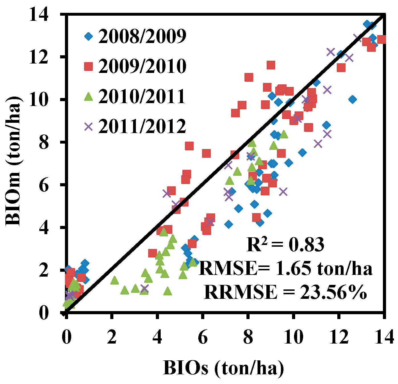
10]. Typically, biomass simulated with the data assimilation method was overestimated when the measured values exceeded 2 ton/ha, but was underestimated when the measured values were less than 2 ton/ha (Figure 3). This explains why the regression equations between NDMI and biomass were similar. Therefore, the integration of spectral indices into the AquaCrop model, using the PSO assimilation algorithm, is a useful tool for winter wheat biomass estimation.
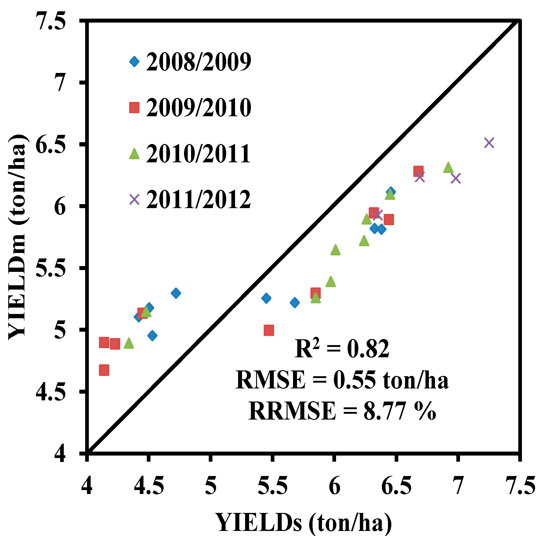
Winter wheat grain yield was simulated according to the optimized values of the initial variables and calibrated crop parameters using the PSO data assimilation algorithm. A good relationship between the measured and simulated yields was found across all four years (R2 = 0.82 and RMSE = 0.55 ton/ha). However, the RRMSE for yield was lower than that for biomass (Table 6 and Table 7), mainly because the latest biomass measurements were taken at the grain filling stage (12 June) rather than at maturity and biomass simulated with the AquaCrop model becomes more accurate with the development of winter wheat [37,61]. Our results are in agreement with those of Wang et al. [61] and Jin et al. [37]. The AquaCrop model considers the effects of interannual variations in weather and field management strategies, as well as interactions between the two, on wheat growth status; therefore, it was used to analyze the nonlinear interannual variability in crop grain yield [36]. The results suggest that the AquaCrop model is an effective tool for deriving crop management strategies, and can be used to simulate biomass and grain yield of winter wheat. First, biomass retrieved from spectral indices is used to calibrate crop biomass simulated with the AquaCrop model. If crop biomass is accurately simulated, it can be used to simulate yield. The simulated yield is finally obtained directly from the AquaCrop model after data assimilation. Simulated grain yield is a useful measurement for informed decision-making regarding national food security issues. However, it is more important to obtain crop growth status information and then to improve field crop management for improving grain yield to ensure national food security, In short, the dynamic simulated biomass of wheat is used to enhance wheat management and decision-making, and then to ensure wheat yield.
The data assimilation accuracy of biomass and grain yield was acceptable according to the R2, RSME, and RRMSE values (Table 6 and Table 7). The results of Dente et al. [19] and Jiang et al. [23] indicated that assimilating remote sensing data (ENVISAT ASAR, MERIS, and HJ-1A/B satellites images) into the CERES-Wheat model with optimization algorithms (variational assimilation algorithm and Ensemble-Based Four-Dimensional Variational algorithm) can improve the estimation accuracy of wheat yield. Huang et al. [25] recently suggested that combining the WOFOST model and remote sensing data (MODIS and Landsat TM images) with a KF algorithm also increases the estimation accuracy of wheat yield. Our results are in agreement with the results of these studies and demonstrate that the combination of the AquaCrop model and spectral indices with a PSO algorithm can be used to enhance the estimation accuracy of winter wheat yield. A good relationship between the simulated and measured yields was found (Figure 4); however, the relationship between measured and simulated biomass was not reliable during each growth stage (Figure 3). This can be attributed to the influence of a large difference in the biomass measurement date on biomass simulation [37], which then introduced uncertainties into the process of data assimilation. However, the yield simulations were consistent during all crop growth stages. Therefore, the data assimilation method can improve crop yield estimations because the AquaCrop model considers the effects of management strategies and environmental factors on winter wheat growth status, based on a plant’s physiological processes. Our results suggest that integrating remote-sensing data into the AquaCrop model is a feasible method for estimating winter wheat biomass and yield.
In this study, the hyperspectral data that were obtained were ground-based data. To improve our model for estimating biomass and yield in winter wheat, and to make it more practical, it is important to estimate the accuracy and stability of the model using hyperspectral satellite data. The current Landsat and Sentinel-2 satellites provide high spatial resolution imagery data (10–60 m) with relatively short revisit periods. Based on this, Landsat and Sentinel-2 sensors have the potential for improved estimates of biomass and yield in winter wheat at regional scales. With the development of unmanned aerial vehicles (UAV), the combination of UAV and hyperspectral imaging data should allow for the timely estimation of the growth status of crops, with high spatial resolution image data at the field and farm scales, in the future. In this study, we only carried out experiments at a single-site, and obtained good results over four years. The method used in this study is transferrable to other sites. The main insights from this study are as follows: (i) The crop parameters of the AquaCrop model for different crops are parameterized to better-simulate different crop biomass and yields, during all growth stages under different environmental conditions and experimental sites; (ii) different crops should be accurately classified using high temporal and spatial resolution image data when this method is applied to regional scales; (iii) PSO will further enhance the advantages of a parallel algorithm to quickly obtain estimated results at regional scales; (iv) corresponding field crop management strategies (such as water and fertilizer management) can then be carried out, based on the estimated crop biomass, resulting in improved crop yields at regional scales; and (v) in addition, this method can be combined with higher temporal and spatial resolution image data and the AquaCrop model to improve field crop management, and then to enhance crop yield at the sub-field and sub-farm scales in the future. The positive results obtained here were based on single-site experiments over four years, however, further experiments should be carried out to adjust crop parameters of the AquaCrop model under water and fertilizer stress treatments to maintain the stability of the simulated results. The effect of the soil parameter variations on the simulated results in the AquaCrop model should be further investigated to better apply it at regional scales. Further studies are needed to verify these results for different crops, and in different ecological areas, as this study was limited to winter wheat in Beijing, China.

5. Conclusions

In this study, the PSO data assimilation algorithm was used to assimilate field spectroscopic data into the AquaCrop model to improve the estimation accuracy of winter wheat yield under different planting dates and irrigation management strategies. The conclusions are as follows: (i) Several spectral indices were highly correlated with biomass in winter wheat. The exponential regression equation between the normalized difference matter index (NDMI) and biomass was the best model for estimating biomass, with R2 and RMSE values of 0.77 and 1.80 ton/ha, respectively; (ii) The data assimilation method (R2 = 0.83 and RMSE = 1.65 ton/ha) achieved more accurate biomass estimations than the spectral index method; (iii) Yield simulated with the data assimilation method was consistent with measured yield across all four years (R2 and RMSE values of 0.82 and 0.55 ton/ha, respectively). In summary, the results indicated that the data assimilation method is an effective method for estimating biomass and yield of winter wheat. The results provide a guideline for optimizing irrigation management strategies for winter wheat in this region.

Acknowledgments

This study was supported by the Natural Science Foundation of China (41601369, 41471285, 41471351, 41301375, 41271345,), the Beijing Natural Science Foundation (4141001), the Special Funds for Technology Innovation Capacity Building, sponsored by the Beijing Academy of Agriculture and Forestry Sciences (KJCX20140417, KJCX20150409), and Yangzhou University Excellent Doctoral Foundation. We are grateful to staff for the collection of field data.

Author Contributions

Xiuliang Jin, Xingang Xu, Guijun Yang, and Jihua Wang conceived of and designed the study; Xiuliang Jin made substantial contributions to the acquisition, analysis, and interpretation of the data; Xiuliang Jin, Zhenhai Li, Xingang Xu, Guijun Yang, and Jihua Wang performed the experiments; Xiuliang Jin and Lalit Kumar discussed the basic structure of the manuscript; and Xiuliang Jin finished the first draft; Lalit Kumar reviewed and edited the draft. All authors have read and approved the submitted manuscript, have agreed to be listed as authors, and have accepted the final version for publication.

Conflicts of Interest

The authors declare no conflicts of interest.

References

  1. Zhang, H.C. Thoughts on cultivation techniques for high quality of wheat in China and its processing. Jiangsu Agric. Sci. 2000, 5, 2–6. (In Chinese) [Google Scholar]
  2. Lobell, D.B.; Asner, G.P.; Ortiz-Monasterio, J.I.; Benning, T.L. Remote sensing of regional crop production in the Yaqui Valley, Mexico: Estimates and uncertainties. Agric. Ecosyst. Environ. 2003, 94, 205–220. [Google Scholar] [CrossRef]
  3. Fang, H.; Liang, S.; Hoogenboom, G.; Teasdale, J.; Cavigelli, M. Corn-yield estimation through assimilation of remotely sensed data into the CSM-CERES-Maize model. Int. J. Remote Sens. 2008, 29, 3011–3032. [Google Scholar] [CrossRef]
  4. Thorp, K.R.; Wang, G.; West, A.L.; Moran, M.S.; Bronson, K.F.; White, J.W.; Mon, J. Estimating crop biophysical properties from remote sensing data by inverting linked radiative transfer and ecophysiological models. Remote Sens. Environ. 2012, 124, 224–233. [Google Scholar] [CrossRef]
  5. Morel, J.; Begue, A.; Todoroff, P.; Martine, J.; Lebourgeois, V.; Petit, M. Coupling a sugarcane crop model with the remotely sensed time series of fIPAR to optimise the yield estimation. Eur. J. Agron. 2014, 61, 60–68. [Google Scholar] [CrossRef]
  6. Curry, R.B. Dynamic simulation of plant growth, I. Development of amodel. Trans. ASABE 1971, 14, 946–959. [Google Scholar] [CrossRef]
  7. Launay, M.; Guerif, M. Assimilating remote sensing data into a crop model to improve predictive performance for spatial applications. Agric. Ecosyst. Environ. 2005, 111, 321–339. [Google Scholar] [CrossRef]
  8. Asseng, S.; Ewert, F.; Rosenzweig, C.; Jones, J.W.; Hatfield, J.L.; Ruane, A.C.; Boote, K.J.; Thorburn, P.J.; Rötter, R.P.; Cammarano, D. Uncertainty in simulating wheat yields under climate change. Nat. Clim. Chang. 2013, 3, 827–832. [Google Scholar] [CrossRef]
  9. Hansen, J.W.; Jones, J.W. Scaling-up crop models for climate variability applications. Agric. Syst. 2000, 65, 43–72. [Google Scholar] [CrossRef]
  10. Dorigo, W.A.; Zurita-Milla, R.; de Wit, A.J.; Brazile, J.; Singh, R.; Schaepman, M.E. A review on reflective remote sensing and data assimilation techniques for enhanced agroecosystem modeling. Int. J. Appl. Earth Obs. Geoinf. 2007, 9, 165–193. [Google Scholar] [CrossRef]
  11. Bacour, C.; Baret, F.; Béal, D.; Weiss, M.; pavageau, K. Neural network estimation of LAI, fAPAR, fCover and LAI × Cab from top of canopy MERIS eflectance data: Principles and validation. Remote Sens. Environ. 2006, 105, 313–325. [Google Scholar] [CrossRef]
  12. Baret, F.; Hagolle, O.; Geiger, B.; Bicheron, P.; Miras, B.; Huc, M.; Berthelot, B.; Nino, F.; Weiss, M.; Samain, O.; et al. LAI, fAPAR and fCOVER cyclopes global products derived from vegetation. Part 1: Principles of the algorithm. Remote Sens. Environ. 2007, 110, 275–286. [Google Scholar] [CrossRef] [Green Version]
  13. Jin, X.L.; Diao, W.Y.; Xiao, C.H.; Wang, F.Y.; Chen, B.; Wang, K.R.; Li, S.K. Estimation of wheat agronomic parameters using new spectral indices. PLoS ONE 2013, 8, e72736. [Google Scholar] [CrossRef] [PubMed]
  14. Jin, X.; Yang, G.; Xu, X.; Yang, H.; Feng, H.; Li, Z.; Shen, J.; Lan, Y.; Zhao, C. Combined Multi-Temporal Optical and Radar Parameters for Estimating LAI and Biomass in Winter Wheat Using HJ and RADARSAR-2 Data. Remote Sens. 2015, 7, 13251–13272. [Google Scholar] [CrossRef]
  15. Jin, X.L.; Wang, K.R.; Xiao, C.H.; Diao, W.Y.; Wang, F.Y.; Chen, B.; Li, S.K. Comparison of two methods for estimation of leaf total chlorophyll content using remote sensing in wheat. Field Crops Res. 2012, 135, 24–29. [Google Scholar] [CrossRef]
  16. Haboudane, D.; Miller, J.R.; Pattey, E.; Zarco-Tejada, P.J.; Strachan, I.B. Hyperspectral vegetation indices and novel algorithms for predicting green LAI of crop canopies: Modeling and validation in the context of precision agriculture. Remote Sens. Environ. 2004, 90, 337–352. [Google Scholar] [CrossRef]
  17. Curnel, Y.; de WitA, J.W.; Duveiller, G.; Defourny, P. Potential performances of remotely sensed LAI assimilation in WOFOST model based on an OSS Experiment. Agric. For. Meteorol. 2011, 151, 1843–1855. [Google Scholar] [CrossRef]
  18. Jarlan, L.; Mangiarotti, S.; Mougin, E.; Mazzega, P.; Hiernaux, P.; Le Dantec, V. Assimilation of SPOT/VEGETATION NDVI into a sahelian vegetation dynamics model. Remote Sens. Environ. 2008, 112, 1381–1394. [Google Scholar] [CrossRef]
  19. Dente, L.; Satlino, G.; Mattia, F.; Rinaldi, M. Assimilation of leaf area index derived from ASAR and MERIS data into CERES-Wheat model to map wheat yield. Remote Sens. Environ. 2008, 112, 1395–1407. [Google Scholar] [CrossRef]
  20. Duveiller, G.; Defourny, P. A conceptual framework to define the spatial resolution requirements for agricultural monitoring using remote sensing. Remote Sens. Environ. 2010, 114, 2637–2650. [Google Scholar] [CrossRef]
  21. Lewis, P.; Gomez-Dans, J.; Kaminski, T.; Settle, J.; Quaife, T.; Gobron, N.; Styles, J.; Berger, M. An earth observation land data assimilation system (EO-LDAS). Remote Sens. Environ. 2012, 120, 219–235. [Google Scholar] [CrossRef]
  22. Ines, A.V.M.; Das, N.N.; Hansen, J.W.; Njoku, E.G. Assimilation of remotely sensed soil moisture and vegetation with a crop simulation model for maize yield prediction. Remote Sens. Environ. 2013, 138, 149–164. [Google Scholar] [CrossRef]
  23. Jiang, Z.; Chen, Z.; Chen, J.; Ren, J.; Li, Z.; Sun, L. The Estimation of Regional Crop Yield Using Ensemble-Based Four-Dimensional Variational Data Assimilation. Remote Sens. 2014, 6, 2664–2681. [Google Scholar] [CrossRef]
  24. Liu, F.; Liu, X.; Ding, C.; Wu, L. The dynamic simulation of rice growth parameters under cadmium stress with the assimilation of multi-period spectral indices and crop model. Field Crops Res. 2015, 183, 225–234. [Google Scholar] [CrossRef]
  25. Huang, J.; Sedano, F.; Huang, Y.; Ma, H.; Li, X.; Liang, S.; Tian, L.; Zhang, X.; Fan, J.; Wu, W. Assimilating a synthetic Kalman filter leaf area index series into the WOFOST model to improve regional winter wheat yield estimation. Agric. For. Meteorol. 2016, 216, 188–202. [Google Scholar] [CrossRef]
  26. Abou-Ismail, O.; Huang, J.; Wang, R. Rice yield estimation by integrating remote sensing with rice growth simulation model. Pedosphere 2004, 14, 519–526. [Google Scholar]
  27. Mo, X.; Liu, S.; Lin, Z.; Xu, Y.; Xiang, Y.; McVicar, T.R. Prediction of crop yield, water consumption and water use efficiency with a SVAT-crop growth model using remotely sensed data on the North China Plain. Ecol. Model. 2005, 183, 301–322. [Google Scholar] [CrossRef]
  28. Thorp, K.R.; Hunsaker, D.J.; French, A.N. Assimilation leaf area index estimates from remote sensing into the simulations of a cropping systems model. Trans. ASABE 2010, 53, 251–262. [Google Scholar] [CrossRef]
  29. Fang, H.; Liang, S.; Hoogenboom, G. Integration of MODIS LAI and vegetation index products with the CSM–CERES–Maize model for corn yield estimation. Int. J. Remote Sens. 2011, 32, 1039–1065. [Google Scholar] [CrossRef]
  30. Li, Y.; Zhou, Q.G.; Zhou, J.; Zhang, G.F.; Chen, C.; Wang, J. Assimilating remote sensing information into a coupled hydrology-crop growth model to estimate regional maize yield in arid regions. Ecol. Model. 2014, 291, 15–27. [Google Scholar] [CrossRef]
  31. Maas, S.J. Use of remotely-sensed information in agricultural crop growth models. Ecol. Model. 1988, 41, 247–268. [Google Scholar] [CrossRef]
  32. Plummer, S.E. Perspectives on combining ecological process models and remotely sensed data. Ecol. Model. 2000, 129, 169–186. [Google Scholar] [CrossRef]
  33. Jongschaap, R.E. Run-time calibration of simulation models by integrating remote sensing estimates of leaf area index and canopy nitrogen. Eur. J. Agron. 2006, 24, 316–324. [Google Scholar] [CrossRef]
  34. Delecolle, R.; Maas, S.J.; Guerif, M.; Baret, F. Remote sensing and crop production models-present trends. ISPRS J. Photogramm. 1992, 47, 145–161. [Google Scholar] [CrossRef]
  35. Liang, S.; Li, X.; Xie, X.H. Land Surface Observation, Modeling and Data Assimilation; Higher Education Press: Beijing, China, 2013. [Google Scholar]
  36. Steduto, P.; Hsiao, T.C.; Raes, D.; Fereres, E. AquaCrop-The FAO crop model to simulate yield response to water. I. Concepts. Agron. J. 2009, 101, 426–437. [Google Scholar] [CrossRef]
  37. Jin, X.L.; Feng, H.K.; Li, Z.H.; Song, S.N.; Zhu, X.K.; Song, X.Y.; Yang, G.J.; Xu, X.G.; Guo, W.S. Assessment of the AquaCrop model for use in simulation of irrigated winter wheat canopy cover, biomass, and grain yield in the North China Plain. PLoS ONE 2014, 9, e86938. [Google Scholar] [CrossRef] [PubMed]
  38. Allen, R.G.; Pereira, L.S.; Raes, D.; Smith, M. Crop Evapotranspiration-Guidelines for Computing Crop Water Requirements; FAO Irrigation and Drainage Paper 56; FAO: Rome, Italy, 1998. [Google Scholar]
  39. Penuelas, J.; Filella, I.; Biel, C.; Serrano, L.; Save, R. The reflectance at the 950–970 nm region as an indicator of plant water status. Int. J. Remote Sens. 1993, 14, 1887–1905. [Google Scholar] [CrossRef]
  40. Seelig, H.D.; Hoehn, A.; Stodieck, L.S.; Klaus, D.M.; Adams, W.W.; Emery, W.J. The assessment of leaf water content using leaf reflectance ratios in the visible, near-, and short-wave-infrared. Int. J. Remote Sens. 2008, 29, 3701–3713. [Google Scholar] [CrossRef]
  41. Hunt, E.R., Jr.; Rock, B.N. Detection of changes in leaf water content using near-and middle-infrared reflectances. Remote Sens. Environ. 1989, 30, 43–54. [Google Scholar]
  42. Wang, L.; Qu, J.J.; Hao, X.; Hunt, E.R. Estimating dry matter content from spectral reflectance for green leaves of different species. Int. J. Remote Sens. 2011, 32, 7097–7109. [Google Scholar] [CrossRef]
  43. Jin, X.L.; Xu, X.G.; Song, X.Y.; Li, Z.H.; Wang, J.H.; Guo, W.S. Estimation of leaf water content in winter wheat using grey relational analysis-partial least squares modeling with hyperspectral data. Agron. J. 2013, 105, 1385–1392. [Google Scholar] [CrossRef]
  44. Jiang, Z.; Huete, A.R.; Didan, K.; Miura, T. Development of a two-band enhanced vegetation index without a blue band. Remote Sens. Environ. 2008, 112, 3833–3845. [Google Scholar] [CrossRef]
  45. Rondeaux, G.; Steven, M.; Baret, F. Optimization of soil-adjusted vegetation indices. Remote Sens. Environ. 1996, 55, 95–107. [Google Scholar] [CrossRef]
  46. Dash, J.; Curran, P.J. The MERIS terrestrial chlorophyll index. Int. J. Remote Sens. 2004, 25, 5403–5413. [Google Scholar] [CrossRef]
  47. Gitelson, A.A.; Viña, A.; Ciganda, V.; Rundquist, D.C. Remote estimation of canopy chlorophyll content in crops. Geophys. Res. Lett. 2005, 32. [Google Scholar] [CrossRef]
  48. Rouse, J.W.; Haas, R.H.; Schell, J.A.; Deering, D.W.; Harlan, J.C. Monitoring the Vernal Advancement of Retrogradation (Green Wave Effect) of Natural Vegetation; Type III, Final Report; NASA: Washington, DC, USA, 1974; pp. 1–371.
  49. Jin, X.L.; Yang, G.J.; Li, Z.H.; Feng, H.K.; Xu, X.G. New combined spectral index to improve total leaf chlorophyll content estimation in cotton. IEEE J. Sel. Top. Appl. Earth Obs. Remote Sens. 2014, 7, 4589–4600. [Google Scholar] [CrossRef]
  50. Gitelson, A.A. Wide dynamic range vegetation index for remote quantification of characteristics of vegetation. J. Plant Physiol. 2004, 161, 165–173. [Google Scholar] [CrossRef] [PubMed]
  51. Brownlee, K.A. Statistical Theory and Methodology in Science and Engineering; John Wiley & Sons: New York, NY, USA, 1956. [Google Scholar]
  52. Raes, D.; Steduto, P.; Hsiao, T.C.; Fereres, E. AquaCrop-The FAO Crop Model to Simulate Yield Response to Water: Reference Manual Annexes. Available online: http://www.fao.org/nr/water/aquacrop.html (accessed on 22 October 2009).
  53. Raes, D.; Steduto, P.; Hsiao, T.C.; Fereres, E. Reference Manual: AquaCrop Plug-in Program (Version 4.0); FAO: Rome, Italy, 2012. [Google Scholar]
  54. Lorite, I.J.; García-Vila, M.; Santos, C.; Ruiz-Ramos, M.; Fereres, E. AquaData and AquaGIS: Two computer utilities for temporal and spatial simulations of water-limited yield with AquaCrop. Comput. Electron. Agric. 2013, 96, 227–237. [Google Scholar] [CrossRef]
  55. Kenndy, J.; Eberhart, R. Particle swarm optimization. In Proceedings of IEEE International Conference on Neural Networks, Perth, Australia, 27 November–1 December 1995; pp. 1942–1948.
  56. Vanuytrecht, E.; Raes, D.; Willems, P. Global sensitivity analysis of yield output from the water productivity model. Environ. Model. Softw. 2014, 51, 323–332. [Google Scholar] [CrossRef]
  57. Wang, H.; Zhu, Y.; Li, W.; Cao, W.; Tian, Y. Integrating remotely sensed leaf area index and leaf nitrogen accumulation with RiceGrow model based on particle swarm optimization algorithm for rice grain yield assessment. J. Appl. Remote Sens. 2014, 8. [Google Scholar] [CrossRef]
  58. Soddu, A.; Deidda, R.; Marrocu, M.; Meloni, R.; Paniconi, C.; Ludwig, R.; Soddea, M.; Mascarob, G.; Perrab, E. Climate variability and durum wheat adaptation using the AquaCrop model in southern Sardinia. Procedia Environ. Sci. 2013, 19, 830–835. [Google Scholar] [CrossRef]
  59. Heng, L.K.; Hsiao, T.C.; Evett, S.; Howell, T.; Steduto, P. Validating the FAO AquaCrop model for irrigated and water deficient field maize. Agron. J. 2009, 101, 488–498. [Google Scholar] [CrossRef]
  60. Jin, X.L.; Yang, G.J.; Li, Z.H.; Xu, X.G.; Wang, J.H.; Lan, Y.B. Estimation of water productivity in winter wheat using the AquaCrop model with field hyperspectral data. Precis. Agric. 2016. [Google Scholar] [CrossRef]
  61. Wang, X.X.; Wang, Q.J.; Fan, J.; Fu, Q.P. Evaluation of the AquaCrop model for simulating the impact of water deficits and different irrigation regimes on the biomass and yield of winter wheat grown on China’s Loess Plateau. Agric. Water Manag. 2013, 129, 95–104. [Google Scholar]
Figure 1. Flowchart of the Particle Swarm Optimization (PSO) assimilation method for the AquaCrop model and remote sensing data.
Remotesensing 08 00972 g001
Figure 2. Regression model between biomass and normalized difference matter index (NDMI) (a); and model validation (b).
Remotesensing 08 00972 g002
Figure 3. Comparison of data assimilation biomass (BIOs) and field measurement biomass (BIOm) values in winter wheat across the four experiments.
Remotesensing 08 00972 g003
Figure 4. Comparison of data assimilation yield (YIELDs) and field measurement yield (YIELDm) values in winter wheat across the four experiments.
Remotesensing 08 00972 g004
Table 1. Winter wheat cultivars and planting dates in 2008, 2009, 2010, and 2011.
Winter Wheat CultivarsPlanting Date
Nongda195, Jingdong8, Jing942828 September, 7 October, and 20 October 2008
Nongda195, Jingdong13, Jing942825 September, 5 October, and 15 October 2009
Nongda195, Yannong19, Jing942825 September, 5 October, and 15 October 2010
Nongda211, Zhongmai175, Jingdong8, Jing984325 September 2011
Note: There were three winter wheat cultivars, and each had three planting dates per year, in 2008, 2009, and 2010. In 2011, four cultivars were planted on the same date.
Table 2. Spectral reflectance measurement dates for 2009, 2010, 2011, and 2012.
Wheat Growth StagesMeasurement Dates
2009201020112012
Jointing16 April 18 April13 April
28 April23 April 28 April
Heading6 May6 May7 May10 May
Anthesis12 May19 May17 May21 May
Grain filling26 May1 June 30 May
10 June7 June
12 June
Table 3. Summary of spectral indices studied.
Spectral IndexNameFormulaReferences
WI IWater index (970, 900)R970/R900[39]
WI IIWater index (1300, 1450)R1300/R1450[40]
NDIINormalized difference infrared index(R850 − R1650)/(R850 + R1650)[41]
NDMINormalized difference matter index(R1649 − R1722)/(R1649 + R1722)[42]
TBWIThree band water index(R973 − R1720)/R1447[43]
EVIEnhanced vegetation index2.5 × (R800 − R660 )/(1 + R800 + 2.4 × R660)[44]
TCARITransformed chlorophyll absorption in reflectance index3 × ((R700 − R670) − 0.2 × (R700 − R550) × (R700/R670))[23]
OSAVIOptimized soil-adjusted vegetation index1.16 × (R800 − R670)/(R800 + R670 + 0.16)[45]
TCARI/OSAVICombined Index IITCARI/OSAVI[16]
MTCIMERIS terrestrial chlorophyll index(R750 − R710)/(R710 − R680)[46]
CIred edgeRed edge model(R750/R720) − 1[47]
NDVINormalized difference vegetation index(R800 − R670)/(R800 + R670)[48]
DCNI IDouble-peak canopy nitrogen index I(R750 − R700)/(R700 − R670)/(R750 − R670 + 0.09)[49]
OSAVI × CIred edgeCombined Index IOSAVI × CIred edge[13]
WDRVIWide dynamic range vegetation indexWDRVI = (α × R800 − R670)/(α × R800 + R670) α = 0.1[50]
Note: Ri denotes reflectance at band i (nanometer).
Table 4. Initial values and ranges of calibration parameters, or initial data, of the AquaCrop model.
VariablesValuesRanges
Canopy growth coefficient (cgc)0.060.05–0.07
Maximum canopy cover in fraction soil cover (ccx)0.650.82–0.99
Canopy decline coefficient (cdc)0.050.04–0.07
Growth degree day: from sowing to emergence (eme)175100–250
Number of plants per hectare (num)4,500,0002,500,000–5,500,000
Soil water depletion factor for canopy senescence (psen)0.650.55–0.75
Shape factor for water stress coefficient for stomatal control (pstoshp)2.51.5–3.5
Growth degree day: from sowing to maximum rooting depth (rootdep)15001200–1800
Table 5. Correlations between biomass and spectral indices of winter wheat (n = 135).
Vegetation IndexRegression EquationsR2FRMSE (Ton/Ha)RRMSE (%)
WI Iy = 1.169x−13.50.72 **0.852.0529.33
WI IIy = 0.264x2.1490.56 **0.622.9842.63
NDIIy = 29.40x1.6200.67 **0.802.2432.04
NDMIy = 0.883e70.06x0.77 **0.941.8025.75
TBWIy = 2.3x1.0400.52 **0.803.4148.78
EVIy = 15.13x1.6600.61 **0.732.9241.77
TCARIy = 28.11x0.8470.38 **0.453.8755.36
OSAVIy = 22.73x3.3520.60 **0.812.8941.34
TCARI/OSAVIy = 1.165x0.3610.30 **0.344.0858.37
MTCIy = 0.451x1.8380.63 **0.772.4835.48
CIred edgey = 3.767x1.7500.68 **0.802.1831.19
NDVIy = 15.33x4.8350.59 **0.732.9542.20
DCNI Iy = 2.626e0.458x0.25 **0.274.4263.23
OSAVI × CIred edgey = 3.704x0.6190.58 **0.782.9642.34
WDRVIy = 4.947e2.533x0.54 **0.713.0343.35
Note: n = number of data pairs; x represents the spectral index; and y represents biomass. In addition, x and e represents power and exponential function in regression equations, respectively. Probability levels of 0.05 and 0.01 are indicated by * and **, respectively; F represents the homoscedasticity value in Levene’s test. If the associated probability for the F test is larger than 0.05, the assumption of homoscedasticity is met.
Table 6. Equations for regressions between data assimilation biomass (BIOs) and field measurement biomass (BIOm) of winter wheat for the four experiments.
YearnRegression EquationsR2FRMSE (Ton/Ha)RRMSE (%)
200954y = 0.847x − 0.1140.810.961.6926.68
201054y = 0.853x + 0.8470.820.781.6724.58
201127y = 0.754x − 0.1980.810.841.5630.65
201220y = 0.863x + 0.1350.870.831.7225.94
2009–2012155y = 0.872x + 0.3100.820.821.7026.57
C/V a135/20 by = 0.865x + 0.0660.830.851.6523.60
Note: a C represents the calibration dataset (2009–2011, n = 135), and V represents the validation dataset (2012, n = 20). The calibration dataset was used to refine the linear regression relationships between the data assimilation biomass (BIOs) and field measurement biomass (BIOm) across three years of experiments. The validation dataset taken in 2012 was used to validate the estimation accuracy of the linear regression equation based on 2009, 2010, and 2011; b R2 was calculated from 135 calibration datasets, and RMSE was calculated from 20 validation datasets; x represents simulated biomass; y represents measured biomass; and F represents the homoscedasticity value for the Levene’s test. If the associated probability for the F test is larger than 0.05, the assumption of homoscedasticity is met.
Table 7. Regression equations between data assimilation yield (YIELDs) and field measurement yield (YIELDm) values of winter wheat across the four experiments.
YearnRegression EquationsR2FRMSE (Ton/Ha)RRMSE (%)
20099y = 0.406x + 3.2250.790.720.519.42
20109y = 0.482x + 2.7750.830.750.5710.69
20119y = 0.481x + 2.7850.810.760.529.29
20124y = 0.583x + 2.2450.890.830.619.79
2009–201231y = 0.490x + 2.7680.850.800.5710.27
C/V a27/4 by = 0.460x + 2.9110.820.760.558.77
Note: a C represents the calibration dataset (2009–2011, n = 27), and V represents the validation dataset (2012, n = 4). The calibration dataset was used to refine the linear regression relationships between the data assimilation yield (YIELDs) and field measurement yield (YIELDm) across three years of experiments. The validation dataset taken in 2012 was used to validate the estimation accuracy of the linear regression equation based on data from 2009, 2010, and 2011; b R2 was calculated from 27 calibration datasets, and RMSE was calculated from 20 validated datasets; x represents simulated biomass; y represents measured biomass; and F represents the homoscedasticity value for the Levene’s test. If the associated probability for the F test is larger than 0.05, the assumption of homoscedasticity is met.

