Article

Long Term Global Surface Soil Moisture Fields Using an SMOS-Trained Neural Network Applied to AMSR-E Data

by
Nemesio J. Rodríguez-Fernández
1,2,*,
Yann H. Kerr
1,
Robin Van der Schalie
3,4,
Amen Al-Yaari
5,
Jean-Pierre Wigneron
5,
Richard De Jeu
3,4,
Philippe Richaume
1,
Emanuel Dutra
2,
Arnaud Mialon
1 and
Matthias Drusch
6
1
Centre d’Etudes Spatiales de la Biosphère Université de Toulouse, Centre National d’Etudes Spatiales (CNES), Centre National de la Recherche Scientifique (CNRS), Institut de Recherche pour le Dévelopement (IRD), 18 av. Edouard Belin, bpi 2801, 31401 Toulouse CEDEX 9, France
2
European Centre for Medium-Range Weather Forecasts (ECMWF), Shinfield Park, RG2 9AX Reading, UK
3
Faculty of Earth and Life Sciences, VU University Amsterdam (VUA), 1081 HV Amsterdam, The Netherlands
4
Transmissivity B.V., Huygensstraat 34, 2201 AZ Noordwijk, The Netherlands
5
Interactions Sol Plante Atmosphére (ISPA), Unité Mixte de Recherche 1391, Institut National de la Recherche Agronomique (INRA), CS 20032, 33882 Villenave d’ornon cedex, France
6
European Space Research and Technology Centre (ESTEC), European Space Agency (ESA), Keplerlaan 1, 2201 AZ Noordwijk, The Netherlands
*
Author to whom correspondence should be addressed.
Remote Sens. 2016, 8(11), 959; https://doi.org/10.3390/rs8110959
Submission received: 19 July 2016 / Revised: 4 November 2016 / Accepted: 9 November 2016 / Published: 18 November 2016

Abstract

:
A method to retrieve soil moisture (SM) from Advanced Scanning Microwave Radiometer—Earth Observing System Sensor (AMSR-E) observations using Soil Moisture and Ocean Salinity (SMOS) Level 3 SM as a reference is discussed. The goal is to obtain longer time series of SM with no significant bias and with a similar dynamical range to that of the SMOS SM dataset. This method consists of training a neural network (NN) to obtain a global non-linear relationship linking AMSR-E brightness temperatures ( T b ) to the SMOS L3 SM dataset on the concurrent mission period of 1.5 years. Then, the NN model is used to derive soil moisture from past AMSR-E observations. It is shown that in spite of the different frequencies and sensing depths of AMSR-E and SMOS, it is possible to find such a global relationship. The sensitivity of AMSR-E T b ’s to soil temperature ( T s o i l ) was also evaluated using European Centre for Medium-Range Weather Forecast Interim/Land re-analysis (ERA-Land) and Modern-Era Retrospective analysis for Research and Applications-Land (MERRA-Land) model data. The best combination of AMSR-E T b ’s to retrieve T s o i l is H polarization at 23 and 36 GHz plus V polarization at 36 GHz. Regarding SM, several combinations of input data show a similar performance in retrieving SM. One NN that uses C and X bands and T s o i l information was chosen to obtain SM in the 2003–2011 period. The new dataset shows a low bias (<0.02 m3/m3) and low standard deviation of the difference (<0.04 m3/m3) with respect to SMOS L3 SM over most of the globe’s surface. The new dataset was evaluated together with other AMSR-E SM datasets and the Climate Change Initiative (CCI) SM dataset against the MERRA-Land and ERA-Land models for the 2003–2011 period. All datasets show a significant bias with respect to models for boreal regions and high correlations over regions other than the tropical and boreal forest. All of the global SM datasets including AMSR-E NN were also evaluated against a large number of in situ measurements over four continents. Over Australia, all datasets show a strong level of agreement with in situ measurements. Models perform better over Europe and mountainous regions in North America. Remote sensing datasets (in particular NN and the Land Parameter Retrieval Model (LPRM)) perform as well as models for other North American sites and perform better than models over the Sahel region.

Graphical Abstract

1. Introduction

Understanding the Earth’s climate and how it is changing is one of the major challenges of the twenty-first century. Climatic patterns can only be reliably detected in time series that are sufficiently long (at least a few decades) because otherwise, natural short-scale variations can hide the longer term trends. Therefore, to understand the climate evolution, a combination of long-term models and observations is needed. Sustained observations from satellites can contribute significantly to this goal, and this is the objective of observational programs, such as the European Spatial Agency (ESA) Climate Change Initiative (CCI) [1]: to provide information on variables that were identified as “essential climate variables” (ECVs) by the Global Climate Observing System (GCOS) in the context of the United Nations Framework Convention on Climate Change (UNFCCC). This is also the goal of numerical re-analyses, such as ERA-Interim [2], which use data assimilation techniques to merge observations and models in an optimal way during long periods of time.
Soil moisture (SM) has been endorsed by the GCOS as an ECV [3], as it affects the water and energy fluxes at the land surface/atmosphere interface [4,5]. Therefore, one of the ESA CCI projects, launched in 2010, focuses on SM. As already mentioned, in order to use SM information for climate modeling, SM datasets spanning long time periods are needed. The ESA SM CCI has developed a strategy [6,7,8,9] that consists of merging a posteriori different SM datasets obtained with different algorithms applied to data from different microwave active and passive sensors. The scaling of the different datasets is done using as a reference a land surface model (such as GLDAS Noah) [6,7].
The Soil Moisture and Ocean Salinity (SMOS) satellite [10] was launched in November 2009, and it is the first mission specifically designed to retrieve SM from space. Many studies have evaluated the SMOS SM dataset in comparison to other remote sensing datasets, models and in situ measurements [11,12,13,14,15,16,17,18,19]. SMOS shows very good global performance although other remote sensing and model products can show better performances at some sites. In any case, datasets from the only two instruments specifically conceived to measure SM, SMOS and Soil Moisture Active Passive (SMAP), compare very well with each other [20,21].
Since the ESA SM CCI started shortly after the SMOS launch, SMOS is not included in the CCI. However, it is important to investigate ways of including SMOS data in the long-term SM datasets and of evaluating the new datasets. One of the advantages of SMOS is that it can observe at a lower frequency (1.4 GHz) than previous instruments, and this frequency is less affected by the vegetation cover [22]. A pertinent first step towards that goal is to study how to obtain a coherent dataset from SMOS and the NASA/JAXA Advanced Scanning Microwave Radiometer (AMSR-E), which operated from 2003–2011. Two approaches have been discussed in the literature: (i) adapting the Land Parameter Retrieval Model (LPRM) algorithm to SMOS data [23]; (ii) using SMOS SM as a reference to compute local linear regression equations linking AMSR-E T b ’s to SMOS SM and recomputing a SM dataset from AMSR-E observations [24]. The present study is devoted to a third approach: using SMOS SM as reference to find a global non-linear regression relationship linking AMSR-E T b ’s to SMOS SM and recomputing an SM dataset from the AMSR-E observations. Preliminary results were presented in [25,26,27].
Neural networks are a very efficient tool for computing global non-linear regressions. Recently, the ESA has released a new SMOS SM near-real-time product computed with neural networks [28]. NNs have been used successfully to retrieve SM from AMSR-E observations over Mongolia, Australia and Italy [29,30]. NNs have also been used to test the a priori merging of active and passive microwaves [31,32], including Advanced Scatterometer (ASCAT) and AMSR-E [33] or ASCAT and SMOS [34]. In contrast, to our knowledge, this is the first time that NNs have been used to extend an SM record in time using a global remote sensing dataset as a reference to train an algorithm to retrieve SM from previous observations by another instrument. The NN training phase can be considered as a consistency check of AMSR-E T b ’s and SMOS SM. It has been proposed that training an NN with a land surface model could be an efficient approach to assimilate satellite data into that same model [31,32]. However, if the goal is creating a generic long-term data record suitable for general data assimilation applications, not using a land surface model to train the NN is a potential advantage as one does not want to assimilate information from one model into another.
The rest of this paper is organized as follows. Section 2 describes the remote sensing and model datasets used. Section 3 presents the in situ measurements used for the evaluation and the comparison protocol. Section 4 discusses the training of the neural networks and the soil moisture retrieval. The new SM dataset is evaluated in Section 5 in comparison to SMOS L3 SM (Section 5.1), other AMSR-E SM datasets (Section 5.2), global models (Section 5.3) and in situ measurements (Section 5.4). Finally, the conclusions are summarized in Section 6.

2. Datasets and Pre-Processing

2.1. SMOS Soil Moisture

SMOS [10,35] was launched on 2 November 2009 to measure the thermal emission from the Earth in the 1.4-GHz protected frequency range in full-polarization and for incidence angles from 0°–∼60°. The footprint (full width at half maximum of the synthesized beam) is ∼43 km on average [35]. The Equator overpass time is 6:00 a.m./p.m. for ascending/descending orbits.
The SMOS SM retrieval algorithm is based on the iterative minimization of the difference of a forward model and the brightness temperatures ( T b ’s) measured by SMOS [36]. The model uses the τ ω (optical depth-single scattering albedo) approach to take into account the effect of vegetation [37]. In the case of forest, two contributions to the opacity are taken into account: one from the arboreous component, which is estimated from the maximum Leaf Area Index (LAI) [38], and another from the understory vegetation. Soil temperature is obtained from ECMWF Integrated Forecast System (IFS) data. For footprints with mixed land cover, the soil moisture content of the minor land cover is estimated from ECMWF IFS, and its contribution to the T b is fixed. For such cases, the SMOS SM retrieval is only performed for the dominant land cover class within the footprint [36]. The Centre Aval de Traitement de Données SMOS (CATDS) Level 3 daily product (SMOS L3 SM, [39]) Version 3.00 was used in this study. The Level 3 algorithm uses three orbits in a seven-day window to constrain the optical depth as it is not physically expected to vary strongly in that time period [39]. CATDS products are provided on an Equal-Area Scalable Earth grid version 2 (EASEv2) with typical node spacing of 25 km [40] as two files per day, one for ascending and another of descending half-orbits (there is no temporal averaging in the L3 daily product).

2.2. AMSR-E Brightness Temperatures

The Advanced Microwave Scanning Radiometer for the Earth Observation System (AMSR-E) is a six-frequency dual-polarized total-power passive microwave radiometer dedicated to observing water-related geophysical parameters [41]. AMSR-E was launched in May 2002, on-board the Aqua satellite, which follows a near-polar Sun-synchronous orbit of 98.8-min periods, crossing the Equator at 1:30 p.m. local time for ascending orbits and at 1:30 a.m. for descending orbits. AMSR-E observed the Earth until October 2011, in six frequency bands: 6.9 GHz (C-band), 10.7 GHz (X-band), 18.7 GHz, 23.8 GHz, 36.5 GHz and 89.0 GHz, at a constant incidence angle of 55°. The footprint size depends on the frequency; for instance, it is (cross-track × along-track) 43 × 75 km2 and 29 × 51 km2 at 6.9 and 10.7 GHz, respectively. The sampling interval on the Earth’s surface is 10.1 km along-track and 9.0 km across-track. In this study, Level 2A brightness temperatures (L2A, Version 12) have been used. The dataset was obtained from the National Snow and Ice Data Center.

2.3. AMSR-E LPRM Soil Moisture

The Land Parameter Retrieval Model (LPRM) is the baseline model for the soil moisture retrievals from the passive microwave sensors within the ESA ECV CCI soil moisture dataset [42]. The SM retrievals from LPRM have been extensively validated [12,43], and the model performance has been documented in numerous publications [6,44]. LPRM demonstrated a good soil moisture retrieval skill from AMSR-E observations over sparse to moderately-vegetated regions [15,45]. LPRM uses vertical and horizontal polarized T b ’s as an input and uses a radiative transfer model to simultaneously solve for SM and vegetation optical depth [6]. An advantage of LPRM is that it can be applied on different frequency bands, including the X, C and L bands. The LPRM SM dataset used in this study was obtained with an optimized single scattering albedo, a new roughness model and using both AMSR-E and SMOS observations [23,46].

2.4. AMSR-E Reg Soil Moisture

The “AMSR-E Reg” SM dataset [24] has been obtained by computing local linear regressions linking the surface reflectivity for vertical and horizontal polarization and SMOS L3 SM using a set of three free parameters for each grid point. The local regression parameters were computed in the June 2010–October 2011 period (when both AMSR-E and SMOS were in operation), getting as many triplets of free parameters as land grid points with available AMSR-E T b ’s and SMOS L3 SM data (∼1.5 × 10⁵ points). In a second step, those parameters are used to estimate SM from AMSR-E observations over the 2003–2010 period.

2.5. ESA Climate Change Initiative Soil Moisture

The European Space Agency Climate Change Initiative (CCI) has supported the generation of a long-term SM product based on multiple microwave sensors in space, such as the radiometers (passive) SMMR (Scanning Multichannel Microwave Radiometer), SSM/I (Special Sensor Microwave Imager), Tropical Rainfall Measuring Mission’s (TRMM) Microwave Imager (TMI), WindSat Polarimetric Radiometer, AMSR-E and AMSR-2 and the active sensors on board the European Remote Sensing (ERS) satellites (Wind Scatterometer) and the Metop satellites (Advanced Scatterometer, ASCAT) [47]. Datasets derived from the different instruments are scaled into a common climatology by matching their cumulative distribution functions (CDF) to those of AMSR-E for the passive datasets or ASCAT for the active datasets. Since the different satellite products are provided in different units, they are scaled into a common level using GLDAS-Noah model simulations. Finally, the active and passive datasets are merged into a combined single dataset. Over areas with low vegetation, the passive one is used, while over areas with moderate vegetation density, the active one is used. In transition areas, if both passive and active data are available, the average is used, otherwise the only available data are used for the final product. The CCI SM dataset used in this study is Version 2.2 (an evaluation against in situ measurements can be found in [9]).

2.6. MERRA Land

The Modern-Era Retrospective analysis for Research and Applications-Land (MERRA-Land) [48] is an atmospheric re-analysis that makes use of the Goddard Earth Observing System model Version 5 and the data assimilation system Version 5.2.0 with an updated precipitation forcing and catchment land surface model compared to the normal MERRA dataset. It was developed by NASA and is available from the beginning of 1980 to the present day. In the current study, the top 2-cm SM is used. The data have a temporal resolution of one hour and a spatial resolution of 1/2° × 2/3°.

2.7. ECMWF ERA-Land Models

ECMWF model simulations of snow depth, soil temperature and soil moisture were used to filter the data and to compare with remote sensing soil moisture measurements. The data used in this study were extracted from a global Tiled ECMWF Scheme for Surface Exchanges over Land (TESSEL) with improved hydrology [49] simulation of surface parameters from 1979–2014. The land surface model has been forced with the atmosphere from the ERA-Interim re-analysis [2]. This dataset will subsequently be referred to as ERA-Land and differs from the ERA-Interim/Land [50] only in the precipitation forcing, which was not rescaled to match Global Precipitation Climatology Project (GPCP) monthly means since GPCP Version 2.1 was not available after 2010. A more recent version of GPCP could have been used, but it was decided to use the original ERA-Interim precipitations in this study. It has a temporal sampling of 6 h and a spatial resolution of 79 km. Only the soil moisture and temperature from the first layer of the model (0–7-cm depth) have been used in the current study.

2.8. Data Collocation and Filtering

The acquisition time difference between AMSR-E and SMOS could be significant for a dynamic variable, such as SM. Therefore, only the night orbits (descending AMSR-E and ascending SMOS) were used to avoid significant differences in the surface SM due to evaporation and convective precipitation during daytime. Possible SM differences induced by precipitation taking place in between AMSR-E and SMOS overpasses were not taken into account, but they will appear in a limited number of points at the global level, and as shown by [32], this should not affect the training. The CCI, MERRA-Land and ERA-Land datasets were spatially interpolated to the EASEv2 grid by the area-overlap weighted average. The data have also been interpolated to the time of AMSR-E acquisitions by linear interpolation. Several filters can be applied to the data:
  • Reference data uncertainty: An upper limit to the SMOS SM data uncertainty has been set for the training phase (data were used when the Dqx parameter is lower than 0.06 m3/m3 and there is less than 30% of forest in the footprint, the FFO parameter).
  • RFI in L-Band: SMOS SM data with a radio frequency interference (RFI) probability higher than 20% (RFI_Prob field) were filtered out.
  • RFI in C or X bands: AMSR-E brightness temperature difference from C-band to X-band for both for H and V polarizations ( T d i f f H , V = T C H , V T X H , V ) should be in the range 10 K T d i f f H , V 5 K . Otherwise, the data are probably affected by RFI from artificial sources as discussed by [51]. Some geophysical phenomena could be identified by this criterion as RFI, for instance when the scattering is important over snow/ice or dry sand surfaces [52]. However, the effect is small, and a number of studies [6,46] have used the criterion by [51]. In addition, in the current study, snow/ice was filtered out before retrieving SM.
  • Frozen soil and snow: The soil temperature from the ERA-Land model should be higher than 274 K to avoid frozen soil (taking into account a temperature uncertainty of ∼ 1 K). The snow depth from ERA-Land should be lower than 1 mm.
All filters from 1–4 have been applied to obtain a clean training subset (Section 4.1). This subset contains ∼ 4.5 × 10⁶ samples, which allows one to study statistical retrieval techniques. For the AMSR-E NN retrieval and evaluation (Section 5.2, Section 5.3 and Section 5.4), only Filters 3 and 4 have been applied, except for the comparison to SMOS L3 in the common period (June 2010–October 2011; Section 5.1), for which Filter 2 was also applied.

3. In Situ Measurements and Evaluation Protocol

The AMSR-E NN SM dataset discussed in this paper, along with those presented above, was evaluated against in situ measurements for a large number of sites. All of the in situ data were obtained from the International Soil Moisture Network [53] except for the Danish Hydrological Observatory (HOBE) and the African Monsoon Multidisciplinary Analysis (AMMA), which have been directly provided by the teams managing the experimental sites. As the C-band radiation detected from space comes from the first few centimeters of the soil, only SM measurements at the 2-, 5- and 8-cm depth range were used. The sites are located in four continents and cover a large spectrum of climate conditions. Table 1 shows a summary of the networks used, and Figure 1 shows their position. The different networks were classified in two main types:
  • Sparse networks: networks with a single site or a larger number of sites located at a distance larger than the AMSR-E footprint. Therefore, one single in situ measurement is compared to the corresponding remote sensing measurement.
  • Dense networks: networks with more than one sensor (Table 1) in a region of several hundred square kilometers (238 km2 in Reynolds Creek or 610 km2 in Little Washita, for instance). Since this surface is smaller than an AMSR-E footprint (∼1500 km2 at the X-band), measurements from individual sensors of the same network can be averaged to have a soil moisture value more representative of the spatial scale of the remote sensing measurement.

3.1. North America

The SCAN (Soil Climate Analysis Network) network contains over 100 sensors/sites [54] and has been widely used to evaluate modeled and remote sensing soil moisture datasets. The sensors are located in agricultural regions with a relatively homogeneous landscape in many cases. The ARM (Atmospheric Radiation Measurement) network is run by the U.S. Department of Energy as part of the Atmospheric Radiation Measurement Climate Research Facility. SNOTEL (SNOw TELemetry) is a network [55] with a large number of stations (420) located mainly in mountainous areas. These networks are sparse networks that contain a large number of sites located at hundreds of kilometers from each other to sample soil moisture conditions at the continental scale. In addition, the United States Department of Agriculture (USDA) Agricultural Research Service (ARS) operates several dense networks. Three of these networks were used in the current study: Little River (LR) in Georgia, Little Washita (LW) in Oklahoma and Reynolds Creek (RC) in Idaho. These three watersheds cover a variety of soil types, crop types and climates. LR is the most humid site with an annual precipitation amount of 1200 mm, mostly covered by row crops and forests. With a sub-humid climate, the LW watershed is mostly used for agricultural activities with wheat crops and grass covers. Finally, RC is located in a mountainous area. Its climate is classified as semiarid, but frozen soils are very frequent in winter. These dense networks have already been used to evaluate AMSR-E and SMOS retrievals [56,57].

3.2. Europe

The Danish Hydrological OBsErvatory (HOBE) network [14,58] is situated in the Skjern River Catchment, and it is a dense network with 30 stations distributed to sample the different soil and environmental conditions on a scale of tenths of kilometers, comparable to the AMSR-E or SMOS footprints. Nearly 80% of this region is under intensive cultivation, intermixed with patches of spruce forest (∼10%), as well as heath/grassland (∼6%). The measurements of the different sensors are averaged before comparing to remote sensing or model SM datasets.
The Red de Estaciones de MEDición de la Humedad def Suelo (REMEDHUS) network [59] is located in a central sector of the Duero basin in Spain. The climate is semiarid continental Mediterranean, and the area is mainly flat covered by agricultural fields with some patchy forest. The sensors are installed horizontally at a depth of 5 cm.
The Lindenberg Meteorological Observatory-Richard Assmann Observatory (MOL-RAO) [60] site is situated close to Berlin, Germany. The Falkenberg site land cover is grassland. In this study, the horizontal probe at a depth of 8 cm has been selected.
Soil Moisture Observing System–Meteorological Automatic Network Integrated Application (SMOSMANIA) [61] is a network of Météo-France. The locations of the stations were chosen to form an Atlantic to Mediterranean transect, north of the Pyrenees mountain range, with the aim of sampling the marked climatic gradient. In this study, the data measured by the probes at a 5-cm depth have been selected.
The Soil Water and Energy Exchange Poland (SWEX Poland) network [62] has been set up in particular to support calibration and validation of SMOS products over wetlands. In the current study, the probes placed horizontally at a 5-cm depth have been selected.
The Upper Danube catchment (UDC) SMOS network is located in southern Germany [63]. The sensors measuring soil moisture at the 5-cm depth layer have been used in the current study.

3.3. Africa

The AMMA-CATCH (African Monsoon Multidisciplinary Analysis - Coupling the Tropical Atmosphere and the Hydrological Cycle) observatory [64] sites in Niger and Benin have been used in this study. The Niger site (with five stations) is mainly tiger bush on the plateaus and fallow savannah and pearl millet crop fields on the sandy slopes (typical Sahelian rain-fed cultivated area). The annual rainfall amount ranges from 300–600 mm. The Benin site is located 400 km south of the Niger site, in a Soudanian climate. The observed annual rainfall is about 1200 mm. The vegetation is woody savannah and tropical forest. These two sites are processed as dense networks, and the soil moisture values have been averaged (five and nine stations for the Niger and Benin sites, respectively) before comparing to remote sensing and model data.
The Danish Natural Science Research Council field site near Dahra in Senegal, West Africa, (hereafter DAHRA, [65]), was established in 2002 to monitor the ecosystem properties of semiarid savannah grassland and their responses to climatic and environmental change. The site experiences a typical Sahelian climate (annual rainfall ranges from 200–600 mm), and land cover is typically Sahelian with grass species and coexisting trees (3% canopy cover). The sensors sampling horizontally at a 5-cm depth were used in this study.
The CARBOAFRICA (full project name: Quantification, understanding and prediction of carbon cycle, and other greenhouse gases, in Sub-Saharan Africa) [66] site is located in central Sudan and has collected meteorological and soil data from 2002–2012. The site is a sparse savannah in a semiarid region. The soil moisture measured by one sensor placed horizontally at a 5-cm depth is used in the current study.

3.4. Australia

Two subsets of the southeast Australia hydrological network (OzNet) have been used in this study. The Murrumbidgee Soil Moisture Monitoring Network (MSMMN) is located in southern New South Wales, Australia [67]. The Murrumbidgee Catchment shows a climate ranging from semiarid to humid. Land use includes dry land and irrigated agriculture, remnant native vegetation and urban areas. Here, the “sparse network” composed by the 18 initial stations providing soil moisture measurements integrated over the 0–8-cm soil layer has been selected because it has provided data since 2001 (hereafter, OzNet 0.00–0.08).
In addition, data from the smaller Yanco, Kyeamba and Adelong Creek catchments, which are located within the Murrumbidgee Catchment, have also been used [68]. The data started in 2006, but these second generation sites are equipped with 0–5-cm depth probes. Data from these sites have been processed as a single sparse network (hereafter, OzNet 0.00–0.05).

3.5. Local Evaluation Strategy

The AMSR-E NN SM (Section 4) and the other SM datasets (Section 2) have been evaluated against in situ measurements at the sites discussed above. RFI, snow and frozen soil filters (3 and 4 in Section 2.8) have been applied to the data. The in situ measurements have been compared to the closest point of the EASEv2 grid. To select a given in situ measurement, a time window of ±30 min around the time of AMSR-E acquisitions has been applied. Data from a given time are used to compute statistics metrics only if an SM value is available for all of the datasets, ensuring that all time series contain exactly the same number of points. A minimum lower limit of 200 points in a time series has been fixed to use the time series to compute the metrics. Table 1 shows the number of sensors that satisfied the previous criteria for each network, and the mean number of points per time series for those sensors. For sparse networks, the metrics are computed sensor by sensor with respect to the closest grid point. Afterwards, the metrics are averaged to show a global estimate of the performances against each network. For dense networks, the measurements of different sensors were provided averaged by the teams managing the in situ networks or by the ISMN. This averaged time series has been compared with the EASEv2 grid point closest to the center of the sensor coordinates.

4. Soil Moisture Retrieval and Sensitivity to Soil Temperature

Figure 2 shows a schematic representation of the methodology used in this study to retrieve an SMOS-like SM dataset from AMSR-E. Data from the 2010–2011 period with the filtering discussed in Section 2.8 for the training phase were used for the NN models to learn the non-linear mapping between AMSR-E T b ’s and SMOS L3 SM. The neural network training itself is described in Section 4.1. Different neural network configurations have been tested. In a second step, one of the neural networks giving the best results is used to retrieve SM from AMSR-E T b ’s in the 2003–2011 period (Section 4.3). Finally, the retrieved dataset trained on SMOS L3 SM (AMSR-E NN SM) has been evaluated with respect to SMOS L3 SM in June 2010–October 2011 (Section 5.1) and with respect to other AMSR-E SM datasets (Section 5.2), global models (Section 5.3) and in situ measurements (Section 5.4) in the 2003–2011 period.

4.1. Neural Network Training

Multi-layer feed-forward neural networks are universal approximators [69], and previous studies have already shown their ability to perform a non-linear mapping from microwave remote sensing observations to soil moisture [31,70,71,72,73]. A training subset with ∼3 × 10⁵ samples was obtained taking one fourth of the available dates and one fourth of the grid points from the filtered training database (Section 2.8). Data from grid points corresponding to in situ measurement sites were also removed from the training subset. A fraction of 60% of the training subset is used for the actual training. An independent fraction of 20% is used to evaluate the NN performances during the training and to stop the training if the performances decrease in the evaluation subset, even if they still increase with the training subset (to avoid over-training). This technique is usually known as “early stopping”. The final independent fraction of 20% of the training subset is used to compute the performances of the trained NN a posteriori. Gradient back-propagation and minimization with the Levenberg–Marquardt algorithm were used. The sensitivity to the initialization of the minimization has been tested, finding that repeating the training with the same data and configuration, the Pearson correlation coefficient (R) of the NN output and the reference SM dataset change by less than 0.01. The same conclusion holds if the training is done with a different data sub-sample. One single hidden layer with five non-linear neurons (hyperbolic tangents) was used, as this is enough to capture the relationship between the input data and the reference SM. Tests with more neurons did not improve the results. The output layer is a single linear neuron. With this architecture, the total number of synaptic weights to fix is ( n inputs + 1 ) n L 1 + ( n L 1 + 1 ) n L 2 , where n inputs is the size of the input vector, n L 1 = 5 is the number of neurons in the first (hidden) layer and n L 2 = 1 is the number of neurons in the second layer. For instance, the total number of free weights is 31 for an input vector with four elements or 66 for an input vector with eleven elements. No signs of overtraining have been found, and the training has been stopped after 30–50 iterations when the mean squared difference of the NN output and the reference SMOS L3 SM is asymptotically approaching a minimum.

4.2. Input Data Sensitivity to Soil Temperature

In a first approximation, the brightness temperature of the Earth at microwave frequencies is the product of the soil temperature by the emissivity, which depends on the dielectric constant of the soil (which is a function of the soil water content). Previous statistical studies have shown that using temperature information as inputs improves the soil moisture retrievals [31,32,34]. Soil temperature information can actually be extracted from the AMSR-E 36-GHz channel and V polarization T B V 37 G H z using the following equation [74,75]:
T s o i l = 0.893 T B V 37 G H z + 44.8
On the other hand, neural networks have proven to be useful to retrieve soil or near-surface temperature (skin temperature) from microwave remote sensing data from instruments, such as the Special Sensor Microwave/Imagers (SSM/I) [76,77,78]. The comprehensive database constructed for the current study was used here to get further insight on the soil temperature information that can be extracted from AMSR-E data. Several NNs have been trained using AMSR-E T b ’s as input and the soil temperature in the first layer of the MERRA-Land and ERA-Land data as a reference.
Table 2 shows that using one single observable as the input, the highest correlation of the NN output and ERA temperature is found for V polarization at 23 GHz (R = 0.91), significantly higher than the score obtained for V polarization at 36 GHz (R = 0.87). Adding more information as inputs, the NN ability to capture the variability of the soil temperature in the numerical weather prediction models increases. For instance, using both polarizations and three bands (18, 23 and 36 GHz), the correlation is 0.95. Interestingly, an input configuration with T b H at 23 GHz and both T b H and T b V at 36 GHz (Mode 7 in Table 2), is the simplest input configuration that gives the highest score in terms of correlation (0.95) with a standard deviation of the difference (STDD) and root mean square difference (RMSD) values close to those obtained using more channels as input (Table 2). Figure 3 shows a scatter plot of the output of Model 7. The same study, but using MERRA-Land soil temperature gives similar results. An in depth study of soil or skin temperature retrieval from AMSR-E channels is out of the scope of this paper; however, the present results suggest that some appropriate combinations of AMSR-E channels and polarizations could give improved results with respect to using only the 36-GHz channel and V polarization.

4.3. Input Data Sensitivity to Soil Moisture

As a first step, the sensitivity of AMSR-E data to SM was studied using a single AMSR-E polarization and frequency band as input to the NN. The highest correlations of the NN output with the SMOS L3 SM were obtained for C-band and X-band. They were found to be low, with values in the range of 0.3–0.4 for both polarizations. Therefore, in a second step, different combinations of polarizations and frequency bands were studied to increase the ability of the NN to capture the variability of the reference SM dataset. In addition, several studies [24,29,34] have shown the interest of computing derived quantities to increase the sensitivity to SM, such as reflectivities Γ = ( 1 T b T s o i l ) , polarization ratios P R = T b H T b V T b H + T b V or “SM linear expectations” (hereafter, I). To compute an SM linear expectation, the highest ( T b m a x ) and lowest ( T b m i n ) brightness temperatures in the time series for a given latitude (λ) and longitude ( ϕ ) grid point are detected. These values are stored in global maps for each polarization and frequency band together with the associated SMOS L3 SM ( S M T b m i n and S M T b m a x ). Using these extreme-values maps, I λ ϕ ( t ) can be computed from AMSR-E T b ’s for each frequency band and polarization for point λ ϕ and at acquisition time t as:
I λ ϕ ( t ) = S M λ ϕ T b m i n + [ S M λ ϕ T b m a x S M λ ϕ T b m i n ] T b λ ϕ ( t ) T b λ ϕ m i n T b λ ϕ m a x T b λ ϕ m i n
Using SM linear expectations limits the coverage to sites where SMOS L3 is available (not affected by RFI) to compute the local extreme values of SM in the reference dataset. In contrast, the linear expectations give information on the dynamic ranges of both the measured T b ’s and the reference SM, and therefore, they help significantly to capture the dynamics of the reference dataset (see below).
Taking into account the six frequency bands and the two polarizations, the T b ’s and derived quantities, the number of possible combinations of data that can be used as input to the NN is very high (>10 million). Of course, not all of them were evaluated, and a mix of physical insight and numerical tests was used to find the best input data configurations. Table 3 shows a summary of the results. Using one single I as input, the Pearson correlation of the NN output and SMOS L3 increases significantly to 0.73 for the C- and X-bands in V polarization and the X-band in H polarization and up to 0.75 for the C-band in H-polarization. This statistical analysis is in agreement with our understanding of the physics of soil emission, as the soil dielectric constant is more sensitive to soil moisture at lower microwave frequencies and horizontal polarization [79]. On the other hand, using all of the available frequency bands led to improved results. The Pearson correlation of the NN output and SMOS L3 SM increases to 0.76 using all T b ’s (Model 18 in Table 3) and to 0.79 using all I’s (Model 19 in Table 3). Interestingly, when using T b ’s and I’s together as input, the ability of the NN to capture the dynamics in the SMOS L3 SM dataset improves significantly as the correlation of the NN output and SMOS L3 increases to 0.85 when using the six frequency bands (Model 17 in Table 3). This is the highest correlation found. However, to find the best trade-off of performances and simplicity, other configurations were tested with an intermediate number of input elements in between those used by Models 1–10 and Model 17.
Taking into account the linear regressions used by Al Yaari et al. [24] linking locally C-band AMSR-E reflectivities and SMOS L3 SM, an NN using as input C-band reflectivities was tested (using soil temperature from ERA-Land, Model 11). However, the correlation of the NN output and SMOS L3 SM is not higher than when just using one single SM linear expectation at the C- or X-band (Models 1, 2, 6, 7). The input configuration used by Santi et al. [29] to train an NN linking SM and T b ’s computed with a radiative transfer model was also tested. They used C-band and 36-GHz V polarization T b ’s, as they are sensitive to SM and T soil , respectively. In addition, they used polarization ratios at 10 and 18 GHz to account for the effect of vegetation on the soil emission. The correlation of the NN output and SMOS SM is 0.75 (Model 12 in Table 3). Therefore, this configuration is not the best to link AMSR-E T b ’s to SMOS L3 SM. Taking into account that the two lower frequency bands are the most sensitive to soil moisture, the four I’s for the C- and X-band and H and V polarizations were tested as inputs (Model 13 in Table 3). The performance score increases to a correlation of 0.77 and an RMSD of 0.078 m3/m3. Adding as input the T b ’s for those bands and both polarizations (Model 14), the scores improve significantly to a correlation of 0.84 and an RMSD of 0.067 m3/m3, which are close to those of Model 17.
Using this configuration with eight elements as a starting point, an automatic method was adopted to add more input elements and to evaluate the scores. Using this approach, more than 103 input data combinations were evaluated. Many configurations were found giving basically the same results of Model 17, but using fewer input elements. For instance, Model 16 uses 14 input elements, and the correlation remains 0.85 (Table 3). A slightly lower correlation of 0.84, but with the same RMSD of 0.066 m3/m3 can be obtained with only 11 input elements, as Model 15 in Table 3. Interestingly, this configuration uses C- and X-band H and V I’s and T b ’s, complemented by T b H at 23 GHz and both T b H and T b V at 36 GHz, which are the bands and polarizations of Model 7 in Table 3. Therefore, they are giving soil temperature information.
As already mentioned, several combinations of the input elements can give the same results. However, Model 15 has the advantage of being relatively simple, giving scores close to the best possible ones and having a clear physical interpretation. Therefore, this is the NN configuration that has been used to invert the AMSR-E data and generate the new AMSR-E NN SM dataset.
Figure 4 shows a scatter plot obtained with the test subset of the training database for Model 15. The SM retrieved with the NN is plotted versus the SMOS L3 SM (note that the density scatter plot has a logarithmic scale; therefore, most of the points are within the inner densest region of the scatter plot). The fact that it is possible to find a single global relationship with a limited amount of parameters (66 for Model 15) linking AMSR-E T b ’s and SMOS L3 SM retrievals shows that in spite of the different characteristics of both instruments, their measurements are in good agreement over most of the globe. Nevertheless, Section 5.1 below discusses some differences as a function of the land cover.

5. Evaluation

The AMSR-E NN SM has been compared to other datasets using classical statistical metrics, such as the mean, the Pearson correlation (R), the bias and the standard deviation of the difference (STDD). The root mean square of the differences (RMSD) is not discussed, as it is a function of the bias and the STDD ( RMSD 2 = STDD 2 + Bias 2 ). In some studies, the STDD is calculated indirectly from the bias and the RMSD and called unbiased-RMSD.
The Pearson correlation was used to compare the long-term (seasonal) dynamics of two SM datasets. In addition, the short-scale dynamics were evaluated by computing the Pearson correlation of the SM anomalies (hereafter, R a ). The SM anomaly at given time t, S M a ( t ) , was computed using a 36-day window centered at t as follows:
S M a ( t ) = S M ( t ) Mean ( S M ( t 18 , t + 18 ) ) STD ( S M ( t 18 , t + 18 ) )
where S M ( t 18 , t + 18 ) represents the ensemble of measurements in the 36-day window.

5.1. Comparison to SMOS L3

As discussed in the Introduction, constructing long time series of essential climate variables, such as SM, is important for climate studies. Due to the limited lifetime of space missions, it is necessary to use different instruments covering different time periods. In the case of AMSR-E and SMOS, it is possible to use the concurrent missions’ period (from June 2010–October 2011) to compare the AMSR-E NN SM and SMOS L3 SM datasets. It is important to ensure that there are no significant biases, nor significant differences in the temporal dynamics of different datasets; therefore, two important metrics are the Pearson correlation and the bias. Nevertheless, other metrics were also computed. For instance, Figure 5 shows maps of the maximum, minimum, mean and standard deviation of both SM datasets. The AMSR-E NN SM shows lower maximum values (Figure 5f) and slightly larger minimum values (Figure 5d) over some regions. This is also seen in the standard deviation maps. The STD of AMSR-E NN SM (Figure 5h) in the Amazon and the boreal regions is significantly lower than that of the SMOS L3 SM dataset (Figure 5g). The underestimation by the NN of the highest SM values in the reference dataset has also been found by previous studies (see, for instance, Figure 2 in [32] or Figure 4 in [31]). This is due to the fact that extreme values are under-represented in the training dataset and have less weight during the training. This behavior is not exclusive of NNs, but it is common to any regression tool. The maximum and minimum values and the STD can be strongly affected by only a few points with extreme values. Therefore, it is interesting to compare other metrics as the mean of both datasets. Actually, the mean SM maps are in very good agreement (Figure 5c,d).
Figure 6 shows maps of some statistic metrics to compare further the AMSR-E NN and SMOS L3 SM datasets. The bias (AMSR-E NN − SMOS L3) is shown in Figure 6c. By construction, the AMSR-E NN should not have a significant global bias with respect to the SMOS L3 dataset used for the training. However, there can be local biases and geographical patterns. For instance, the AMSR-E NN dataset is drier than SMOS L3 in the areas of tropical forest. The absolute value of the bias is lower than 0.05 m3/m3, which is comparable to the uncertainty level of the SM retrievals [36]. In Australia, Northern Africa, Western Europe, Central Asia, Argentina and large parts of North America, the bias is close to zero (<0.02 m3/m3). Similarly, the STDD (Figure 6d) is lower than 0.04 m3/m3, except in the tropical forest and to a minor extent in the boreal forest.
The seasonal dynamics were compared using maps of the Pearson correlation of AMSR-E NN SM and SMOS L3 SM. The correlation (Figure 6a) shows a similar behavior to the STDD, with high values, except over dense forest regions. Therefore, the SMOS L3 and the AMSR-E NN SM datasets show similar seasonal dynamics. The main difference with respect to the bias and the STDD is found in the northeast African desert, where the correlation is low, but the bias and STDD are also low. In this region of low intrinsic variability of the SM signal, the low correlation could be due to the fact that the variance is not dominated by an annual cycle, but by noise, whose origin could be RFI, implying that RFI pollution could extend beyond the currently filtered area (blank region in the map).
A map of the Pearson correlation of the anomalies, R a , is shown in Figure 6b. The values of R a are lower than those of R (Figure 6a), as expected, since the seasonal cycle is removed, but the two maps show the same patterns, and the AMSR-E NN SM and SMOS-L3 SM anomalies are in good agreement in North America, Australia, parts of Europe, such as the Iberian Peninsula, and regions in Central Asia, Africa and South America.
Regarding the forest areas, one should bear in mind that retrieving soil moisture under dense forest is a problem in itself, and many retrieval algorithms do not perform inversion in these regions, in addition, microwave signals at frequencies of the C- and X-bands or higher are significantly affected by vegetation water content, and it is likely that the AMSR-E signals arising from these regions are not emitted by the soil; even at the L-band, the signals will be strongly affected by the vegetation. In summary, one can conclude that the NN discussed in Section 4, with only 66 free parameters to map globally the relationship from AMSR-E T b ’s to SMOS L3 SM, gives an SM dataset that is very compatible to the SMOS L3 SM used as a reference, except in the regions of very dense forest.

5.2. Comparison to Other AMSR-E SM Datasets

The new AMSR-E NN SM dataset has also been evaluated in the 2003–2011 period against the new version of LPRM [23] (Section 2.2). The results are shown in Figure 7. The correlation of both datasets (Figure 7a) is high ( R > 0.6 ), except at the locations of dense tropical or boreal forests and the Sahara desert. Globally, the good correlation confirms that the dynamic signatures in both datasets are similar and driven by the dynamics of the AMSR-E T b ’s signal, for all but the regions where the dynamics of the T b ’s are small.
In order to compare also the absolute values of both AMSR-E datasets, the bias and the STDD were computed, and they are shown in Figure 7a,c, respectively. The AMSR-E NN SM dataset is on average drier than the AMSR-E LPRM SM dataset. This bias is expected, as the SMOS L3 SM used as a reference to calibrate the global non-linear regression has been found to be drier than previous versions of AMSR LPRM SM [15,80]. The STDD of both products is low (<0.04 m3/m3) over most of the globe, but increases in forested areas up to values of ∼0.08 m3/m3 (Figure 7c). Further evaluation of both products by comparison with the ERA-Land and MERRA-Land datasets is presented in Section 5.3.

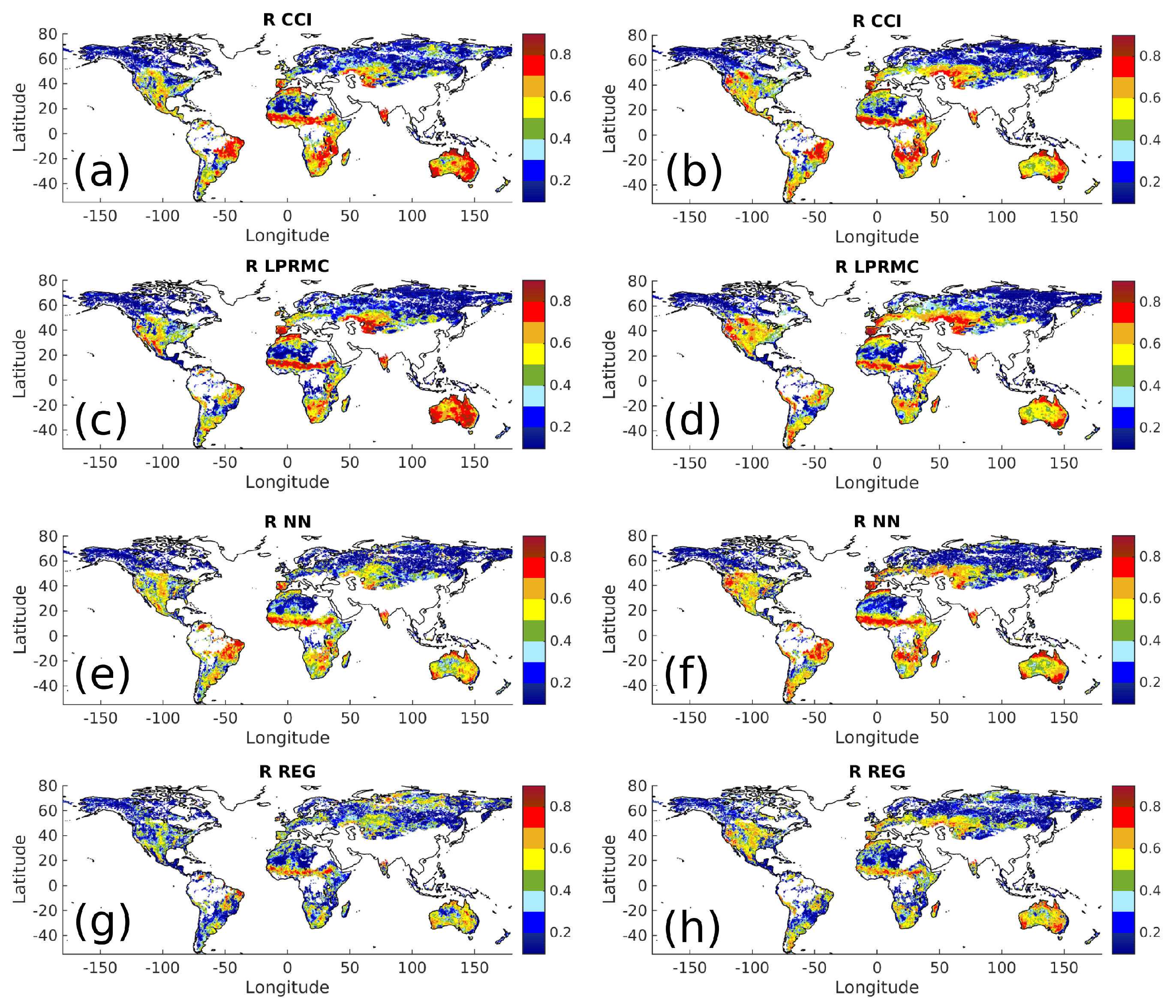
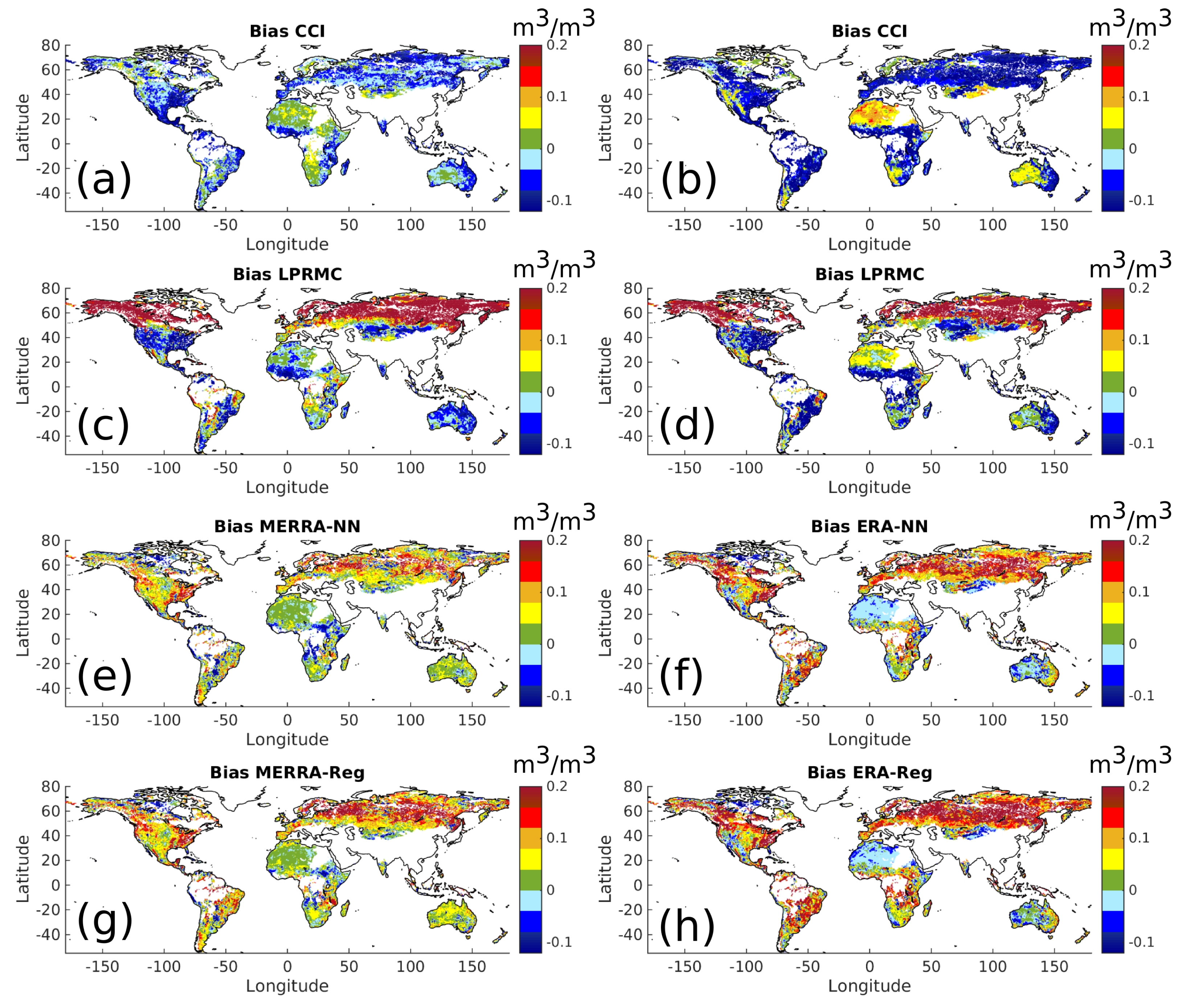
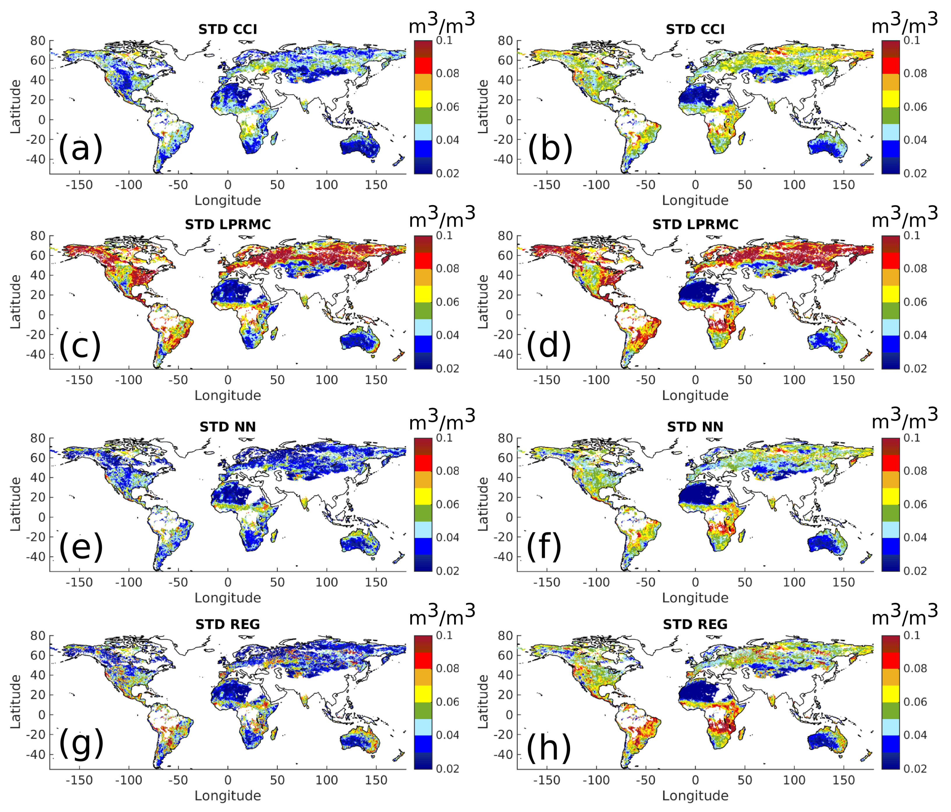
5.3. Global Evaluation against Model Data

To get further insight into the characteristics of the new AMSR-E NN dataset, it was compared to MERRA-Land and ERA-Land model data. The same comparison has been done for other AMSR-E SM datasets and for the CCI SM data.
Firstly, the temporal signatures have been compared by computing the Pearson correlation of both AMSR-E datasets with respect to the two model datasets (Figure 8). The temporal variations of SM in the four remote sensing datasets (AMSR-E NN, AMSR-E Reg, AMSR-E LPRM and CCI) are in good agreement, as they show similar spatial patterns. AMSR-E Reg SM shows higher correlation with model data at high latitudes, in particular with respect to MERRA-Land (Figure 8g); otherwise, the correlation with model data is in general lower than that of other remote sensing datasets. LPRM shows a widespread high correlation with MERRA-Land over Australia (Figure 8c); in contrast, all remote sensing datasets show a more inhomogeneous correlation with respect to ERA-Land in this region (Figure 8b,d,f,h). On the other hand, the correlation is significantly higher with ERA-Land over North America. It is also noteworthy that the correlation maps of AMSR-E LPRM SM and SMOS L3 SM with respect to the ECMWF-DAS2 product (H-TESSEL model with ASCAT SM data assimilation) discussed in [15] show similar spatial patterns.
In addition to the temporal signatures, in order to compare the absolute values, the STDD and the bias were also computed. It has been shown above that AMSR-E NN is in general drier than AMSR-E LPRM. Figure 9 shows that both ERA and MERRA models are, in general, in between AMSR-E NN and AMSR-E LPRM. The same behavior has previously been found for SMOS L3 and AMSR-E LPRM with respect to ECMWF-DAS2 [15]. The CCI dataset shows a low bias with respect to MERRA (Figure 9a), but one should bear in mind that the SM datasets used to compute this product have been re-scaled using a model as a reference.
The STDD shows a significant spatial patterns and values close to 0.1 m3/m3 for LPRM with respect to both MERRA and ERA (Figure 10a,b), in particular for latitudes above ∼45°. The STDD computed for the other three products is significantly lower, in particular with respect to MERRA-Land for AMSR-E Reg and NN (Figure 10e,g), with STDD lower than 0.05 m3/m3 for most of the globe. The lower bias with respect to MERRA in comparison to ERA could be related to a shallower top soil layer in MERRA (0–2 cm) compared to ERA (0–7 cm).

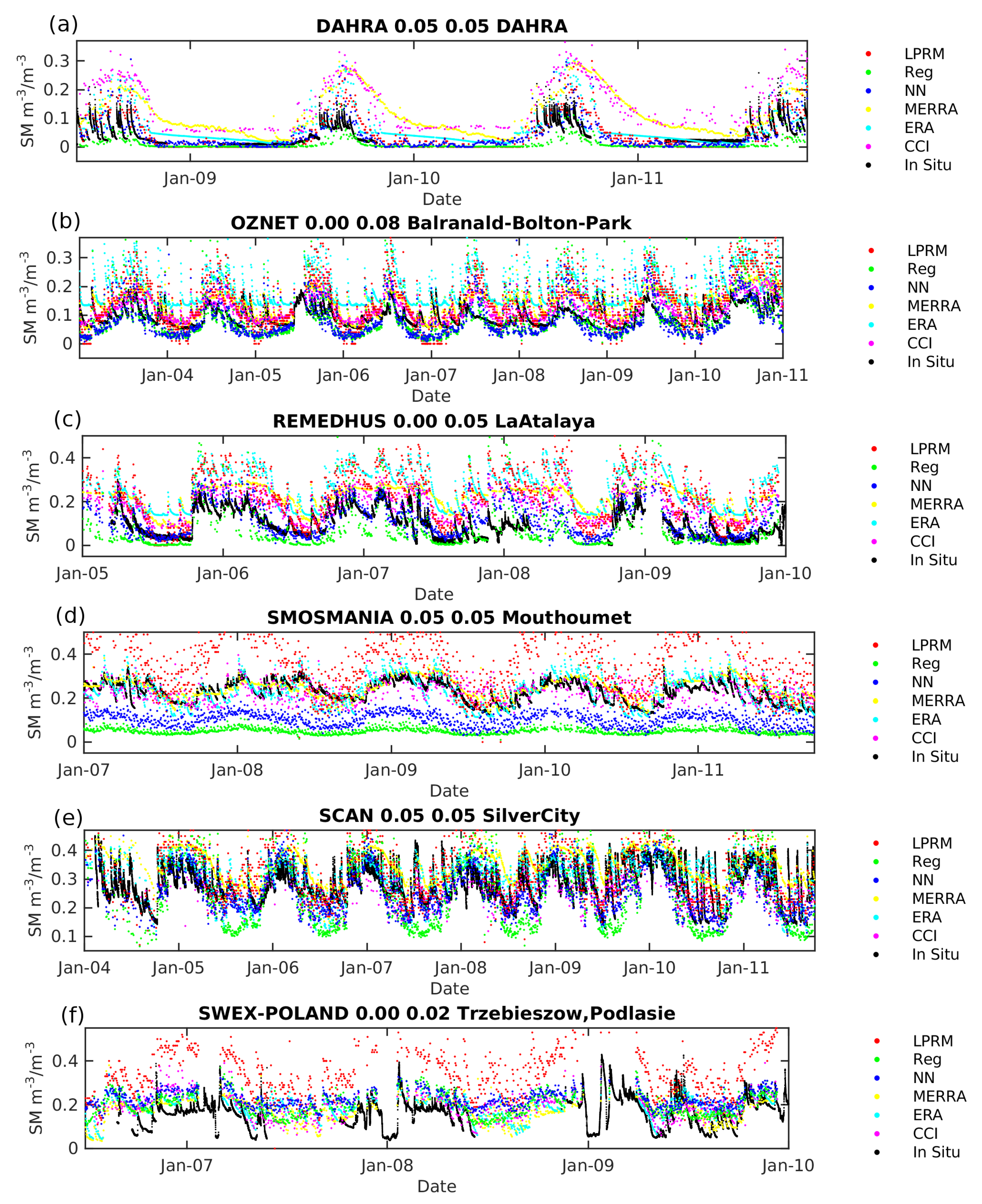
5.4. Local Evaluation against In Situ Measurements

The AMSR-E SM datasets, together with the model datasets, were evaluated against in situ measurements using the database and the protocol discussed in Section 3. Figure 11 shows six time series from the over 400 that have been computed. These time series show the dynamics and absolute values of the four remote sensing products, the two models and the in situ measurements compared in this study.
For each site, the STDD, R and bias with respect to the in situ measurement have been computed. The results are summarized in Table 4. Firstly, it is interesting to remark that the results for the AMSR-E LPRM and Reg SM and for the CCI SM compare well to other studies carried out using the same data, even if the time period of the evaluation protocol is not exactly the same [9,24,46,81].
With respect to sites in Europe (REMEDHUS, SMOSMANIA, UDC-SMOS, SWEX-Poland, HOBE, MOL-RAO), the best scores in terms of correlation are obtained by the ERA-Land model. MERRA-Land also shows better correlation than remote sensing products for some networks, but lower values for other networks. The fact that the ERA-Land model performs best in this region can be due to the fact that in Europe, models are well constrained by a dense network of in situ observations and, on the other hand, to the fact that there are RFI sources that could degrade the quality of the remote sensing products. With respect to the remote sensing products, the best correlations are found for LPRM and NN. In terms of STDD and bias, AMSR-E NN gives the best agreement with the in situ measurements.
The situation is different in the Sahel (AMMA, DAHRA, CARBOAFRICA), where the correlation is significantly better for remote sensing products than for model products. This can be partially attributed to the precipitation that drives the models. For example ERA-Interim is known to have significant problems representing the West Africa Monsoon [82]. The best remote sensing product in this region is LPRM, which gives high correlation values for the four networks, while the performances of other products are more variable. In terms of bias, the best datasets are the two SMOS-based ones, AMSR-E Reg and NN. AMSR-E Reg also gives the lowest STDD for two of the four networks. In these regions, the surface-atmosphere coupling is strong [4], but there are few in situ observations. The positive results of the remote sensing products show the interest of assimilating these data into numerical weather prediction models.
All of the products perform very well for the OzNet networks in Australia, correctly reproducing the temporal evolution of the in situ time series (Pearson correlations 0.7–0.8), in particular when comparing with sensors sampling the 0–5-cm depth. Correlations remain high when comparing with the 0–8-cm sensors, except for AMSR-E NN and Reg.
In North America, the dataset showing the best correlations is ERA-Land. Both models show higher correlations than remote sensing data for mountainous networks (SNOTEL and Reynolds Creek) and SCAN. In Little Washita, AMSR-E NN and CCI show a correlation close to ERA-Land (0.70–0.72 versus 0.76), while in Little River LPRM, AMSR-E Reg, NN and ERA-Land show very similar correlation. AMSR-E NN shows the lowest mean STDD for most networks.

6. Conclusions

A methodology to retrieve SM from AMSR-E has been discussed and evaluated. The method consists of searching for a global non-linear relationship linking AMSR-E T b ’s and SMOS L3 SM to recompute an SM dataset from AMSR-E observations with no significant bias and a similar dynamical range to that of the SMOS L3 dataset. This study differs from that of Al Yaari et al. [24] in that they calibrated point per point a simple linear regression using a physical-based equation. Here, a single global relation was studied. It has been shown that by using neural networks, it is possible to find such a single relationship mapping the space from AMSR-E T b ’s to SMOS L3 SM. Therefore, in spite of the different frequencies and sensing depths of AMSR-E and SMOS, the latter SM dataset and the former T b ’s are in good agreement. To our knowledge, this is the first time that a global SM dataset derived from remote sensing observations has been used as a reference to train a neural network using past satellite mission observations.
It has been shown that the new AMSR-E dataset compares well with the SMOS L3 SM dataset (within the typical error interval of the SMOS L3 SM). In particular, the bias is smaller than 0.04 m3/m3 by construction, with no need of a third-party dataset to perform a bias-correction or to apply any a posteriori statistical correction. This SMOS-based AMSR-E has been evaluated globally, along with other AMSR-E SM datasets and the CCI SM dataset, the MERRA-Land and ERA-Land models. The NN SM dataset show similar features with respect to models as the other remote sensing datasets. All of the AMSR-E SM datasets show a significant bias for boreal forest regions, in particular the LPRM one. LPRM shows the best agreement with MERRA in terms of correlation over Australia. The three AMSR-E datasets show a better agreement in terms of correlation with ERA-Land over North America. The two SMOS-based AMSR-E datasets (NN and Reg) show a lower STTD and bias than LPRM in many regions.
The AMSR-E SM NN dataset has also been evaluated against in situ measurements of soil moisture in a large number of sites (over 400). The same evaluation has been performed for the CCI SM, MERRA-Land, ERA-Land, AMSR-E LPRM and AMSR-E Reg. Models compare better to in situ measurements over Europe, in particular ERA-Land. This could be due to the large number of measurements constraining the numerical weather prediction models in this region and to the fact that the remote sensing observations could be polluted by artificial emission. In contrast, in the Sahel area, remote sensing datasets show better statistics than models, in particular AMSR-E LPRM, in terms of correlation and AMSR-E NN in terms of bias and STDD. These results suggest the potential added value of assimilating remote sensing data into models (numerical weather predictions models, reanalysis, hydrological models) in this region due to the lack of in situ observations and the convective nature of precipitation. Moreover, this region has been also linked with a strong land-atmosphere coupling, which provides a further motivation to better constrain soil moisture evolution using remote sensing data.
Over Australia, all SM products show a similar very good agreement with in situ measurements. In North America, MERRA and ERA models show higher correlations with in situ measurements over mountainous regions, but remote sensing datasets, in particular AMSR-E LPRM and NN, show similar statistics for the other networks.
In summary, the approach studied in this paper is a promising method to re-compute an SM dataset from a passive radiometer using as reference data an SM dataset produced with a different radiometer to obtain longer, consistent by construction, datasets.

Acknowledgments

This research has been partly funded by ESA European Space Research Insitute (ESRIN) under Contract IPL-PSO/FF/vb/13.886 EXPRO+ and by the TOSCA (Terre Ocean Surface Continental Atmosphère) program of “Centre National d’Etudes Spatiales” (CNES, France). The authors thank Patricia de Rosnay and Gianpaolo Balsamo from ECMWF for providing the ERA-Land data and useful comments, respectively. SMOS L3 data were obtained from the “Centre Aval de Traitement des Données SMOS” (CATDS), operated for the CNES (France) by “Institut Français de Recherche pour l’Exploitation de la Mer” (IFREMER) (Brest, France). The authors thank Tom Spain (Dept. of Education, University of Oxford) for his help with the English language editing.

Author Contributions

N.J.R.-F. and Y.H.K. are the principal authors of this manuscript. The neural network approach was designed by N.J.R.-F. with significant contributions from P.R. A.A.-Y. and J.-P.W. provided the AMSR-E Reg data. R.v.d.S. and R.d.J. provided the AMSR-E brightness temperatures and LPRM and CCI soil moisture datasets. E.D. computed the ERA-Land reanalysis until year 2014. A.M. provided SMOS-L3 data. M.D. reviewed the system design and the results. All authors contributed to the inter-comparison of the different soil moisture datasets, participated in the writing and provided comments and suggestions.

Conflicts of Interest

The authors declare no conflict of interest.

References

  1. Hollmann, R.; Merchant, C.; Saunders, R.; Downy, C.; Buchwitz, M.; Cazenave, A.; Chuvieco, E.; Defourny, P.; de Leeuw, G.; Forsberg, R.; et al. The ESA climate change initiative: Satellite data records for essential climate variables. Bull. Am. Meteorol. Soc. 2013, 94, 1541–1552. [Google Scholar] [CrossRef]
  2. Dee, D.; Uppala, S.; Simmons, A.; Berrisford, P.; Poli, P.; Kobayashi, S.; Andrae, U.; Balmaseda, M.; Balsamo, G.; Bauer, P.; et al. The ERA-Interim reanalysis: Configuration and performance of the data assimilation system. Q. J. R. Meteorol. Soc. 2011, 137, 553–597. [Google Scholar] [CrossRef]
  3. Global Climate Observing System (GCOS). Report of the Sixtheen Session of the Steering Committee for the Global Climate Observing System; Technical Report; WMO, IOC, UNEP, ICSU, Report 124; Global Climate Observing System: Geneva, Switzerland, 2008. [Google Scholar]
  4. Koster, R.D.; Dirmeyer, P.A.; Guo, Z.; Bonan, G.; Chan, E.; Cox, P.; Gordon, C.; Kanae, S.; Kowalczyk, E.; Lawrence, D.; et al. Regions of strong coupling between soil moisture and precipitation. Science 2004, 305, 1138–1140. [Google Scholar] [CrossRef] [PubMed]
  5. Tuttle, S.; Salvucci, G. Empirical evidence of contrasting soil moisture—Precipitation feedbacks across the United States. Science 2016, 352, 825–828. [Google Scholar] [CrossRef] [PubMed]
  6. Owe, M.; de Jeu, R.; Holmes, T. Multisensor historical climatology of satellite-derived global land surface moisture. J. Geophys. Res. 2008, 113, F01002. [Google Scholar] [CrossRef]
  7. Liu, Y.; Parinussa, R.; Dorigo, W.; de Jeu, R.; Wagner, W.; Van Dijk, A.; McCabe, M.; Evans, J. Developing an improved soil moisture dataset by blending passive and active microwave satellite-based retrievals. Hydrol. Earth Syst. Sci. 2011, 15, 425–436. [Google Scholar] [CrossRef] [Green Version]
  8. Dorigo, W.A.; de Jeu, R.A.M.; Chung, D.; Parinussa, R.M.; Liu, Y.Y.; Wagner, W.; Fernandez-Prieto, D. Evaluating global trends (1988–2010) in harmonized multi-satellite surface soil moisture. Geophys. Res. Lett. 2012, 39, 18. [Google Scholar] [CrossRef]
  9. Dorigo, W.; Gruber, A.; de Jeu, R.; Wagner, W.; Stacke, T.; Loew, A.; Albergel, C.; Brocca, L.; Chung, D.; Parinussa, R.; et al. Evaluation of the ESA CCI soil moisture product using ground-based observations. Remote Sens. Environ. 2015, 162, 380–395. [Google Scholar] [CrossRef]
  10. Kerr, Y.H.; Waldteufel, P.; Wigneron, J.P.; Martinuzzi, J.; Font, J.; Berger, M. Soil moisture retrieval from space: The Soil Moisture and Ocean Salinity (SMOS) mission. IEEE Trans. Geosci. Remote Sens. 2001, 39, 1729–1735. [Google Scholar] [CrossRef]
  11. Al Bitar, A.; Leroux, D.; Kerr, Y.H.; Merlin, O.; Richaume, P.; Sahoo, A.; Wood, E. Evaluation of SMOS soil moisture products over continental US using the SCAN/SNOTEL network. IEEE Trans. Geosci. Remote Sens. 2012, 50, 1572–1586. [Google Scholar] [CrossRef] [Green Version]
  12. Wanders, N.; Karssenberg, D.; Bierkens, M.; Parinussa, R.; de Jeu, R.; van Dam, J.; de Jong, S. Observation uncertainty of satellite soil moisture products determined with physically-based modeling. Remote Sens. Environ. 2012, 127, 341–356. [Google Scholar] [CrossRef]
  13. Albergel, C.; Calvet, J.C.; de Rosnay, P.; Balsamo, G.; Wagner, W.; Hasenauer, S.; Naeimi, V.; Martin, E.; Bazile, E.; Bouyssel, F.; et al. Cross-evaluation of modeled and remotely sensed surface soil moisture with in situ data in southwestern France. Hydrol. Earth Syst. Sci. Discuss. 2010, 7, 4291–4330. [Google Scholar] [CrossRef]
  14. Bircher, S.; Skou, N.; Kerr, Y.H. Validation of SMOS L1C and L2 products and important parameters of the retrieval algorithm in the Skjern River Catchment, Western Denmark. IEEE Trans. Geosci. Remote Sens. 2013, 51, 2969–2985. [Google Scholar] [CrossRef] [Green Version]
  15. Al-Yaari, A.; Wigneron, J.P.; Ducharne, A.; Kerr, Y.; de Rosnay, P.; de Jeu, R.; Govind, A.; Al Bitar, A.; Albergel, C.; Munoz-Sabater, J.; et al. Global-scale evaluation of two satellite-based passive microwave soil moisture datasets (SMOS and AMSR-E) with respect to Land Data Assimilation System estimates. Remote Sens. Environ. 2014, 149, 181–195. [Google Scholar] [CrossRef] [Green Version]
  16. Al-Yaari, A.; Wigneron, J.P.; Ducharne, A.; Kerr, Y.; Wagner, W.; de Lannoy, G.; Reichle, R.; Al Bitar, A.; Dorigo, W.; Richaume, P.; et al. Global-scale comparison of passive (SMOS) and active (ASCAT) satellite based microwave soil moisture retrievals with soil moisture simulations (MERRA-Land). Remote Sens. Environ. 2014, 152, 614–626. [Google Scholar] [CrossRef] [Green Version]
  17. Leroux, D.J.; Kerr, Y.H.; Al Bitar, A.; Bindlish, R.; Jackson, T.J.; Berthelot, B.; Portet, G. Comparison between SMOS, VUA, ASCAT, and ECMWF soil moisture products over four watersheds in US. IEEE Trans. Geosci. Remote Sens. 2014, 52, 1562–1571. [Google Scholar] [CrossRef] [Green Version]
  18. Louvet, S.; Pellarin, T.; al Bitar, A.; Cappelaere, B.; Galle, S.; Grippa, M.; Gruhier, C.; Kerr, Y.; Lebel, T.; Mialon, A.; et al. SMOS soil moisture product evaluation over West-Africa from local to regional scale. Remote Sens. Environ. 2015, 156, 383–394. [Google Scholar] [CrossRef]
  19. Kerr, Y.H.; Al-Yaari, A.; Rodriguez-Fernandez, N.; Parrens, M.; Molero, B.; Leroux, D.; Bircher, S.; Mahmoodi, A.; Mialon, A.; Richaume, P.; et al. Overview of SMOS performance in terms of global soil moisture monitoring after six years in operation. Remote Sens. Environ. 2016, 180, 40–63. [Google Scholar] [CrossRef]
  20. Jackson, T.; O’Neill, P.; Njoku, E.S.C.; Bindlish, R.; Colliander, A.; Chen, F.; Burgin, M.; Dunbar, S.; Piepmeier, J.; Cosh, M.; et al. Calibration and Validation for the L2/3-SM-P Version 3 Data Products; Technical Report; SMAP Project, JPL D-93720; Jet Propulsion Laboratory: Pasadena, CA, USA, 2016. [Google Scholar]
  21. Burgin, M.; Colliander, A.; Njoku, E.G.; Cabot, F.; Kerr, Y.; Bindlish, R.; Jackson, T.; Entekhabi, D.; Yueh, S. A comparative study of the SMAP passive soil moisture product with existing satellite-based soil moisture products. IEEE Trans. Geosci. Remote Sens. 2016, in press. [Google Scholar]
  22. Ulaby, F.T.; Moore, R.K.; Fung, A.K. Microwave Remote Sensing Active and Passive-Volume III: From Theory to Applications; Artech House, Inc.: Norwood, MA, USA, 1986. [Google Scholar]
  23. Van der Schalie, R.; Kerr, Y.; Wigneron, J.; Rodríguez-Fernández, N.; Al-Yaari, A.; de Jeu, R. Global SMOS soil moisture retrievals from the land parameter retrieval model. Int. J. Appl. Earth Observ. Geoinf. 2016, 45, 125–134. [Google Scholar] [CrossRef]
  24. Al-Yaari, A.; Wigneron, J.; Kerr, Y.; De Jeu, R.; Rodriguez-Fernandez, N.; van der Schalie, R.; Al Bitar, A.; Mialon, A.; Richaume, P.; Dolman, A. Testing regression equations to derive long-term global soil moisture datasets from passive microwave observations. Remote Sens. Environ. 2016, 180, 453–464. [Google Scholar] [CrossRef]
  25. Rodríguez-Fernández, N.J.; Kerr, Y.H.; de Jeu, R.A.; van der Schalie, R.; Wigneron, J.P.; Ayaari, A.A.; Dolman, H.; Drusch, M.; Mecklenburg, S. Long time series of soil moisture obtained using neural networks: Application to AMSR-E and SMOS. In Proceedings of the EGU General Assembly Conference, Vienna, Austria, 12–17 April 2015; Volume 17, p. 10250.
  26. Rodríguez-Fernández, N.J.; Kerr, Y.; Wigneron, J.; Al-Yaari, A.; de Jeu, R.; van der Schalie, R.; Richaume, P.; Drusch, A.J.; Drusch, M.; Mecklenburg, S. Eleven-years of an homogeneous soil moisture dataset from AMSR-E and SMOS observations. In Proceedings of 2015 International Geoscience and Remote Sensing Symposium IGARSS, Milan, Italy, 26–31 July 2015.
  27. Van der Schalie, R.; de Jeu, R.; Kerr, Y.; Wigneron, J.P.; Rodríguez-Fernández, N.; Al-Yaari, A.; Drusch, M.; Mecklenburg, S.; Dolman, H. Evaluation of three different data fusion approaches that uses satellite soil moisture from different passive microwave sensors to construct one consistent climate record. In Proceedings of the EGU General Assembly Conference, Vienna, Austria, 17–22 April 2016; Volume 18, p. 8520.
  28. Mecklenburg, S.; Drusch, M.; Kaleschke, L.; Rodriguez-Fernandez, N.; Reul, N.; Kerr, Y.; Font, J.; Martin-Neira, M.; Oliva, R.; Daganzo-Eusebio, E.; et al. ESA’s soil moisture and ocean salinity mission: From science to operational applications. Remote Sens. Environ. 2016, 180, 3–18. [Google Scholar] [CrossRef]
  29. Santi, E.; Pettinato, S.; Paloscia, S.; Pampaloni, P.; Macelloni, G.; Brogioni, M. An algorithm for generating soil moisture and snow depth maps from microwave spaceborne radiometers: HydroAlgo. Hydrol. Earth Syst. Sci. Discuss. 2012, 9, 3851–3900. [Google Scholar] [CrossRef]
  30. Santi, E.; Paloscia, S.; Pettinato, S.; Brocca, L.; Ciabatta, L. Robust assessment of an operational algorithm for the retrieval of soil moisture from AMSR-E data in Central Italy. IEEE J. Sel. Top. Appl. Earth Obs. Remote Sens. 2016, 9, 2478–2492. [Google Scholar] [CrossRef]
  31. Aires, F.; Prigent, C.; Rossow, W.B. Sensitivity of satellite microwave and infrared observations to soil moisture at a global scale: 2. Global statistical relationships. J. Geophys. Res. 2005, 110, D07110. [Google Scholar] [CrossRef]
  32. Jiménez, C.; Clark, D.B.; Kolassa, J.; Aires, F.; Prigent, C. A joint analysis of modeled soil moisture fields and satellite observations. J. Geophys. Res. Atmos. 2013, 118, 6771–6782. [Google Scholar] [CrossRef]
  33. Kolassa, J.; Gentine, P.; Prigent, C.; Aires, F. Soil moisture retrieval from AMSR-E and ASCAT microwave observation synergy. Part 1: Satellite data analysis. Remote Sens. Environ. 2016, 173, 1–14. [Google Scholar] [CrossRef]
  34. Rodríguez-Fernández, N.J.; Aires, F.; Richaume, P.; Kerr, Y.H.; Prigent, C.; Kolassa, J.; Cabot, F.; Jiménez, C.; Mahmoodi, A.; Drusch, M. Soil moisture retrieval using neural networks: Application to SMOS. IEEE Trans. Geosci. Remote Sens. 2015, 53, 5991–6007. [Google Scholar] [CrossRef]
  35. Kerr, Y.; Waldteufel, P.; Wigneron, J.P.; Delwart, S.; Cabot, F.; Boutin, J.; Escorihuela, M.J.; Font, J.; Reul, N.; Gruhier, C.; et al. The SMOS Mission: New tool for monitoring key elements of the Global Water Cycle. Proc. IEEE 2010, 98, 666–687. [Google Scholar] [CrossRef] [Green Version]
  36. Kerr, Y.; Waldteufel, P.; Richaume, P.; Wigneron, J.; Ferrazzoli, P.; Mahmoodi, A.; Al Bitar, A.; Cabot, F.; Gruhier, C.; Juglea, S.; et al. The SMOS soil moisture retrieval algorithm. IEEE Trans. Geosci. Remote Sens. 2012, 50, 1384–1403. [Google Scholar] [CrossRef]
  37. Wigneron, J.P.; Kerr, Y.; Waldteufel, P.; Saleh, K.; Escorihuela, M.J.; Richaume, P.; Ferrazzoli, P.; de Rosnay, P.; Gurney, R.; Calvet, J.C.; et al. L-band Microwave Emission of the Biosphere (L-MEB) Model: Description and calibration against experimental data sets over crop fields. Remote Sens. Environ. 2007, 107, 639–655. [Google Scholar] [CrossRef]
  38. Ferrazzoli, P.; Guerriero, L.; Wigneron, J.P. Simulating L-band emission of forests in view of future satellite applications. IEEE Trans. Geosci. Remote Sens. 2002, 40, 2700–2708. [Google Scholar] [CrossRef]
  39. Kerr, Y.; Jacquette, E.; Al Bitar, A.; Cabot, F.; Mialon, A.; Richaume, P.; Quesney, A.; Berthon, L. CATDS SMOS L3 Soil Moisture Retrieval Processor, Algorithm Theoretical Baseline Document (ATBD); Technical Report SO-TN-CBSA-GS-0029; Ifremer: Brest, France, 2013. [Google Scholar]
  40. Brodzik, M.J.; Billingsley, B.; Haran, T.; Raup, B.; Savoie, M.H. Incremental but Significant Improvements for Earth-Gridded Data Sets. ISPRS Int. J. Geo-Inf. 2014, 3, 1154–1156. [Google Scholar] [CrossRef]
  41. Kawanishi, T.; Sezai, T.; Ito, Y.; Imaoka, K.; Takeshima, T.; Ishido, Y.; Shibata, A.; Miura, M.; Inahata, H.; Spencer, R.W. The advanced microwave scanning radiometer for the earth observing system (AMSR-E), NASDA’s contribution to the EOS for global energy and water cycle studies. IEEE Trans. Geosci. Remote Sens. 2003, 41, 184–194. [Google Scholar] [CrossRef]
  42. Liu, Y.; Dorigo, W.; Parinussa, R.; de Jeu, R.; Wagner, W.; McCabe, M.; Evans, J.; van Dijk, A. Trend-preserving blending of passive and active microwave soil moisture retrievals. Remote Sens. Environ. 2012, 123, 280–297. [Google Scholar] [CrossRef]
  43. Wagner, W.; Naeimi, V.; Scipal, K.; de Jeu, R.; Martínez-Fernández, J. Soil moisture from operational meteorological satellites. Hydrogeol. J. 2007, 15, 121–131. [Google Scholar] [CrossRef]
  44. De Jeu, R.A.; Holmes, T.R.; Parinussa, R.M.; Owe, M. A spatially coherent global soil moisture product with improved temporal resolution. J. Hydrol. 2014, 516, 284–296. [Google Scholar] [CrossRef]
  45. De Jeu, R.; Wagner, W.; Holmes, T.; Dolman, A.; van de Giesen, N.; Friesen, J. Global soil moisture patterns observed by space borne microwave radiometers and scatterometers. Surv. Geophys. 2008, 29, 399–420. [Google Scholar] [CrossRef] [Green Version]
  46. Van der Schalie, R.; de Jeu, R.; Kerr, Y.; Wigneron, J.; Rodríguez-Fernández, N.; Al-Yaari, A.; Mecklenburg, S.; Drusch, M. A radiative transfer based approach towards the merging of SMOS and AMSR-E soil moisture retrievals into one consistent climate data record. Remote Sens. Environ. 2016, in press. [Google Scholar]
  47. Wagner, W.; Dorigo, W.; de Jeu, R.; Fernandez, D.; Benveniste, J.; Haas, E.; Ertl, M. Fusion of active and passive microwave observations to create an essential climate variable data record on soil moisture. In Proceedings of the 22th International Society for Photogrammetry and Remote Sensing (ISPRS) Congress, Melbourne, Australia, 25 August–1 September 2012; Volume 25.
  48. Reichle, R.H.; Koster, R.D.; de Lannoy, G.J.; Forman, B.A.; Liu, Q.; Mahanama, S.P.; Touré, A. Assessment and enhancement of MERRA land surface hydrology estimates. J. Clim. 2011, 24, 6322–6338. [Google Scholar] [CrossRef]
  49. Balsamo, G.; Beljaars, A.; Scipal, K.; Viterbo, P.; van den Hurk, B.; Hirschi, M.; Betts, A.K. A revised hydrology for the ECMWF model: Verification from field site to terrestrial water storage and impact in the Integrated Forecast System. J. Hydrometeorol. 2009, 10, 623–643. [Google Scholar] [CrossRef]
  50. Balsamo, G.; Albergel, C.; Beljaars, A.; Boussetta, S.; Brun, E.; Cloke, H.; Dee, D.; Dutra, E.; Muñoz-Sabater, J.; Pappenberger, F.; et al. ERA-Interim/Land: A global land surface reanalysis data set. Hydrol. Earth Syst. Sci. 2015, 19, 389–407. [Google Scholar] [CrossRef]
  51. Li, L.; Njoku, E.G.; Im, E.; Chang, P.S.; Germain, K.S. A preliminary survey of radio-frequency interference over the US in Aqua AMSR-E data. IEEE Trans. Geosci. Remote Sens. 2004, 42, 380–390. [Google Scholar] [CrossRef]
  52. Njoku, E.G.; Ashcroft, P.; Chan, T.K.; Li, L. Global survey and statistics of radio-frequency interference in AMSR-E land observations. IEEE Trans. Geosci. Remote Sens. 2005, 43, 938–947. [Google Scholar] [CrossRef]
  53. Dorigo, W.; Wagner, W.; Hohensinn, R.; Hahn, S.; Paulik, C.; Xaver, A.; Gruber, A.; Drusch, M.; Mecklenburg, S.; Oevelen, P.V.; et al. The International Soil Moisture Network: A data hosting facility for global in situ soil moisture measurements. Hydrol. Earth Syst. Sci. 2011, 15, 1675–1698. [Google Scholar] [CrossRef]
  54. Schaefer, G.; Cosh, M.; Jackson, T. The USDA natural resources conservation service soil climate analysis network (SCAN). J. Atmos. Ocean. Technol. 2007, 24, 2073–2077. [Google Scholar] [CrossRef]
  55. Leavesley, G.; David, O.; Garen, D.; Lea, J.; Marron, J.; Pagano, T.; Perkins, T.; Strobel, M. A modeling framework for improved agricultural water supply forecasting. In Proceedings of the AGU 2008 Fall Meeting, San Francisco, CA, USA, 15–19 December 2008; Volume 1.
  56. Jackson, T.J.; Cosh, M.H.; Bindlish, R.; Starks, P.J.; Bosch, D.D.; Seyfried, M.; Goodrich, D.C.; Moran, M.S.; Du, J. Validation of advanced microwave scanning radiometer soil moisture products. IEEE Trans. Geosci. Remote Sens. 2010, 48, 4256–4272. [Google Scholar] [CrossRef]
  57. Jackson, T.J.; Bindlish, R.; Cosh, M.H.; Zhao, T.; Starks, P.J.; Bosch, D.D.; Seyfried, M.; Moran, M.S.; Goodrich, D.C.; Kerr, Y.H.; et al. Validation of Soil Moisture and Ocean Salinity (SMOS) soil moisture over watershed networks in the US. IEEE Trans. Geosci. Remote Sens. 2012, 50, 1530–1543. [Google Scholar] [CrossRef] [Green Version]
  58. Bircher, S.; Skou, N.; Jensen, K.H.; Walker, J.P.; Rasmussen, L. A soil moisture and temperature network for SMOS validation in Western Denmark. Hydrol. Earth Syst. Sci. 2012, 16, 1445–1463. [Google Scholar] [CrossRef] [Green Version]
  59. Martínez-Fernández, J.; Ceballos, A. Mean soil moisture estimation using temporal stability analysis. J. Hydrol. 2005, 312, 28–38. [Google Scholar] [CrossRef]
  60. Beyrich, F.; Adam, W. Site and Data Report for the Lindenberg Reference Site in CEOP—Phase I; Technical Report; Reports of the Deutscher Wetterdiens, Report 230; Selbstverlag des Deutschen Wetterdienstes: Offenbach am Main, Germany, 2007. [Google Scholar]
  61. Calvet, J.C.; Fritz, N.; Froissard, F.; Suquia, D.; Petitpa, A.; Piguet, B. In situ soil moisture observations for the CAL/VAL of SMOS: The SMOSMANIA network. In Proceedings of the IEEE International Geoscience and Remote Sensing Symposium 2007 (IGARSS 2007), Barcelona, Spain, 23–28 July 2007; pp. 1196–1199.
  62. Marczewski, W.; Slominski, J.; Slominska, E.; Usowicz, B.; Usowicz, J.; Romanov, S.; Maryskevych, O.; Nastula, J.; Zawadzki, J. Strategies for validating and directions for employing SMOS data, in the Cal-Val project SWEX (3275) for wetlands. Hydrol. Earth Syst. Sci. Discuss. 2010, 7, 7007–7057. [Google Scholar] [CrossRef]
  63. Dall’Amico, J.T.; Schlenz, F.; Loew, A.; Mauser, W. SMOS soil moisture validation: Status at the upper Danube Cal/Val site eight months after launch. In Proceedings of the 2010 IEEE International Geoscience and Remote Sensing Symposium (IGARSS), Honolulu, HI, USA, 25–30 July 2010; pp. 3801–3804.
  64. Lafore, J.P.; Flamant, C.; Giraud, V.; Guichard, F.; Knippertz, P.; Mahfouf, J.F.; Mascart, P.; Williams, E. Introduction to the AMMA Special Issue on ‘Advances in understanding atmospheric processes over West Africa through the AMMA field campaign’. Q. J. R. Meteorol. Soc. 2010, 136, 2–7. [Google Scholar] [CrossRef]
  65. Tagesson, T.; Fensholt, R.; Guiro, I.; Rasmussen, M.O.; Huber, S.; Mbow, C.; Garcia, M.; Horion, S.; Sandholt, I.; Holm-Rasmussen, B.; et al. Ecosystem properties of semiarid savanna grassland in West Africa and its relationship with environmental variability. Glob. Chang. Biol. 2015, 21, 250–264. [Google Scholar] [CrossRef] [PubMed]
  66. Ardö, J. A 10-year dataset of basic meteorology and soil properties in Central Sudan. Dataset Pap. Sci. 2013, 2013, 297973. [Google Scholar] [CrossRef]
  67. Smith, A.B.; Walker, J.P.; Western, A.W.; Young, R.I.; Ellett, K.M.; Pipunic, R.C.; Grayson, R.B.; Siriwardena, L.; Chiew, F.H.S.; Richter, H. The Murrumbidgee soil moisture monitoring network data set. Water Resour. Res. 2012, 48, W07701. [Google Scholar] [CrossRef]
  68. Young, R.; Walker, J.; Yeoh, N.; Smith, A.; Ellett, K.; Merlin, O.; Western, A. Soil Moisture and Meteorological Observations From the Murrumbidgee Catchment; Technical Report; Department of Civil and Environmental Engineering, The University of Melbourne: Parkville, Australia, 2008. [Google Scholar]
  69. Hornik, K.; Stinchcombe, M.; White, H. Multilayer feedforward networks are universal approximators. Neural Netw. 1989, 2, 359–366. [Google Scholar] [CrossRef]
  70. Paloscia, S.; Macelloni, G.; Santi, E.; Tedesco, M. The capability of microwave radiometers in retrieving soil moisture profiles: An application of artificial neural networks. In Proceedings of the 2002 IEEE International Geoscience and Remote Sensing Symposium (IGARSS’02), Toronto, ON, Canada, 24–28 June 2002; pp. 1390–1393.
  71. Liu, S.F.; Liou, Y.A.; Wang, W.J.; Wigneron, J.P.; Lee, J.B. Retrieval of crop biomass and soil moisture from measured 1.4 and 10.65 GHz brightness temperatures. IEEE Trans. Geosci. Remote Sens. 2002, 40, 1260–1268. [Google Scholar]
  72. Angiuli, E.; del Frate, F.; Monerris, A. Application of neural networks to soil moisture retrievals from L-band radiometric data. In Proceedings of 2008 IEEE International Geoscience and Remote Sensing Symposium, Boston, MA, USA, 8–11 July 2008; Volume 2, pp. 61–64.
  73. Notarnicola, C.; Angiulli, M.; Posa, F. Soil moisture retrieval from remotely sensed data: Neural network approach versus bayesian method. IEEE Trans. Geosci. Remote Sens. 2008, 46, 547–557. [Google Scholar] [CrossRef]
  74. Holmes, T.R.H.; de Jeu, R.A.M.; Owe, M.; Dolman, A.J. Land surface temperature from Ka band (37 GHz) passive microwave observations. J. Geophys. Res. Atmos. 2009, 114, D04113. [Google Scholar] [CrossRef]
  75. Holmes, T.; Crow, W.; Hain, C.; Anderson, M.; Kustas, W. Diurnal temperature cycle as observed by thermal infrared and microwave radiometers. Remote Sens. Environ. 2015, 158, 110–125. [Google Scholar] [CrossRef]
  76. Prigent, C.; Rossow, W.R. Retrieval of surface and atmospheric parameters over land from SSM/I: Potential and limitations. Q. J. R. Meteorol. Soc. 1999, 125, 2379–2400. [Google Scholar] [CrossRef]
  77. Aires, F.; Prigent, C.; Rossow, W.B.; Rothstein, M. A new neural network approach including first guess for retrieval of atmospheric water vapor, cloud liquid water path, surface temperature, and emissivities over land from satellite microwave observations. J. Geophys. Res. Atmos. 2001, 106, 14887–14907. [Google Scholar] [CrossRef]
  78. Prigent, C.; Jimenez, C.; Aires, F. Toward “all weather,” long record, and real-time land surface temperature retrievals from microwave satellite observations. J. Geophys. Res. Atmos. 2016, 121, 5699–5717. [Google Scholar] [CrossRef]
  79. Ulaby, F.; Batlivala, P.; Dobson, M. Microwave backscatter dependence on surface roughness, soil moisture, and soil texture: Part I-bare soil. IEEE Trans. Geosci. Electron. 1978, 16, 286–295. [Google Scholar] [CrossRef]
  80. Leroux, D.J.; Kerr, Y.H.; Wood, E.F.; Sahoo, A.K.; Bindlish, R.; Jackson, T.J. An approach to constructing a homogeneous time series of soil moisture using SMOS. IEEE Trans. Geosci. Remote Sens. 2014, 52, 393–405. [Google Scholar] [CrossRef] [Green Version]
  81. Albergel, C.; Dorigo, W.; Balsamo, G.; Muñoz-Sabater, J.; de Rosnay, P.; Isaksen, L.; Brocca, L.; de Jeu, R.; Wagner, W. Monitoring multi-decadal satellite earth observation of soil moisture products through land surface reanalyses. Remote Sens. Environ. 2013, 138, 77–89. [Google Scholar] [CrossRef]
  82. Di Giuseppe, F.; Molteni, F.; Dutra, E. Real-time correction of ERA-Interim monthly rainfall. Geophys. Res. Lett. 2013, 40, 3750–3755. [Google Scholar] [CrossRef]
Figure 1. Locations of the in situ sensors.
Remotesensing 08 00959 g001
Figure 2. Schema of the methodology used in this study.
Remotesensing 08 00959 g002
Figure 3. Scatter plot of the soil temperature retrieved with the neural network using T b H at 23 GHz and both T b H and T b V at 36 GHz (Model 7 in Table 2) versus ERA-Land soil temperature in the first layer (0–7 cm). The scatter plot is represented as the density of points in a logarithmic scale.Scatter plot of the soil temperature retrieved with the neural network versus ERA-Land soil temperature
Remotesensing 08 00959 g003
Figure 4. Scatter plot of the AMSR-E SM retrieved with the neural network (Model 15 in Table 3) versus SMOS L3 SM. The scatter plot is represented as the density of points in a logarithmic scale.
Remotesensing 08 00959 g004
Figure 5. Maps of different statistics metrics for the SMOS L3 SM dataset (left panels) and AMSR-E NN SM (right panels) computed from June 2010–October 2011: minimum values (a,b); mean (c,d); maximum (e,f); and standard deviation (g,h).
Remotesensing 08 00959 g005
Figure 6. Comparison of AMSR-E NN SM and SMOS L3 SM from June 2010–October 2011. (a) Local Pearson correlation of the two SM datasets; (b) local Pearson correlation of the anomalies of the two SM datasets; (c) bias (mean AMSR-E NN SM minus mean SMOS L3 SM); (d) standard deviation of the difference of the two SM datasets.
Remotesensing 08 00959 g006
Figure 7. Comparison of AMSR-E NN SM and AMSR-E LPRM (applied to the C-band) from January 2003–October 2011. (a) Bias (mean of Land Parameter Retrieval Model (LPRM) SM minus the mean of NN SM); (b) Pearson correlation; (c) standard deviation of the difference of both datasets.
Remotesensing 08 00959 g007
Figure 8. Pearson correlation of remote sensing products with respect to Modern-Era Retrospective analysis for Research and Applications-Land (MERRA-Land) (left panels) and ERA-Land (right panels). The remote sensing products evaluated are, from top to bottom: ESA CCI (a,b); AMSR-E LPRM C-Band (c,d); AMSR-E NN (e,f); and AMSR-E Reg (g,h).
Remotesensing 08 00959 g008
Figure 9. Bias of remote sensing products with respect to MERRA-Land (left panels) and ERA-Land (right panels). The remote sensing products evaluated are, from top to bottom: ESA CCI (a,b); AMSR-E LPRM C-Band (c,d); AMSR-E NN (e,f); and AMSR-E Reg (g,h). The bias has been computed as the mean of the remote sensing data minus the mean of model data, except for AMSR-E Reg and NN, for which the bias shown is the mean of the model data minus the mean of the remote sensing data.
Remotesensing 08 00959 g009
Figure 10. Standard deviation of the difference of remote sensing products with respect to MERRA-Land (left panels) and ERA-Land (right panels). The remote sensing products evaluated are, from top to bottom: ESA CCI (a,b); AMSR-E LPRM C-Band (c,d); AMSR-E NN (e,f); and AMSR-E Reg (g,h).
Remotesensing 08 00959 g010
Figure 11. (af) Examples of time series: in situ measurements (black), AMSR-E NN (blue), AMSR-E LPRM (red), AMSR-E Reg (green), CCI (magenta), ERA-Land (cyan) and MERRA-Land (yellow).
Remotesensing 08 00959 g011
Table 1. In situ networks used in this study. The depths are quoted as two numbers: the first one is the upper depth, and the second one is the lower depth of the sensor. Both numbers are equal when the sensor is placed horizontally. The third column gives the number of sensors remaining for each network after applying all of the criteria used for the evaluation that are discussed in Section 3. The third column gives the average number of points in the times series for each network that satisfies the evaluation criteria.
NetworkDepth (cm)SitesPointsLocation
Sparse Networks
ARM0.05–0.0538687USA
CARBOAFRICA0.05–0.051522Sudan
DAHRA0.05–0.051492Senegal
OZNET0.00–0.0523630Australia
OZNET0.00–0.08161168Australia
REMEDHUS0.00–0.0525988Spain
MOL-RAO0.08–0.0811323Germany
SMOSMANIA0.05–0.0514576France
SWEX-POLAND0.05–0.053380Poland
UDC-SMOS0.05–0.0521348Germany
SCAN0.05–0.0588588USA
SNOTEL0.05–0.05147459USA
Dense Networks
ARS Little River0.00–0.0529817USA
ARS Little Washita0.00–0.0520483USA
ARS Reynolds Creek0.00–0.0519954USA
HOBE0.00–0.0532204Denmark
AMMA Benin0.05–0.059381Benin
AMMA Niger0.05–0.055380Niger
Table 2. Evaluations of the performances of different NNs using Advanced Scanning Microwave Radiometer Earth (AMSR-E) T b ’s as input to retrieve the soil temperature (T) as predicted by ERA-Land models. Column 1 shows the model label. Columns 2 and 3 show the Pearson correlation and the root mean square difference of the NN T with respect to ERA-Land T. Column 4 shows the elements of the input vector in terms of polarizations (H or V) and frequency bands (number in GHz). The correlation uncertainty due to the training is 0.01 (Section 4.1).
ModelRRMSDInput Data
10.863.73 T b : V18
20.913.12 T b : V23
30.873.67 T b : V36
40.556.21 T b : H18
50.695.38 T b : H23
60.595.97 T b : H36
70.952.36 T b : V36, H23, H36
80.952.26 T b : V18, V23, H23, H36
90.952.25 T b : V18, V23, V36, H18, H23, H36
Table 3. Evaluations of the performances of the AMSR-E NN soil moisture (SM) with respect to the SMOS L3 SM reference data. Column 1 shows the model label. Columns 2 and 3 show the Pearson correlation and the root mean square difference of the NN SM with respect to SMOS SM. Column 4 shows the elements of the input vector: T b ’s, SM linear expectations I or reflectivity Γ = ( 1 T b T s o i l ) for different polarizations (H or V) and frequency bands (number in GHz) or polarization ratios P R = T b H T b V T b H + T b V for different frequency bands (number in GHz). The correlation uncertainty due to the training is 0.01 (Section 4.1).
ModelRRMSDInput Data
10.740.082I: V6
20.730.083I: V10
30.720.085I: V18
40.720.085I: V23
50.710.086I: V36
60.750.082I: H6
70.730.084I: H10
80.710.086I: H18
90.700.087I: H23
100.710.087I: H36
110.730.084Γ: H6, V6
120.750.081 T b : V6, V36; P R : 10, 18
130.770.078I: H6, V10, V6, V10
140.840.067I & T b : H6, H10, V6, V10
150.840.066I: H6, H10, V6, V10 ; T b : H6, H10, V6, V10, H23, H36, V36
160.850.066I: H6, H10, H18, V6, V10, V18; T b : H6, H18, H23, V6, V18, V23, V36, H10
170.850.065I & T b : H6, H10, H18, H23, H36, H89, V6, V10, V18, V23, V36, V89
180.760.079 T b : H6, H10, H18, H23, H36, H89, V6, V10, V18, V23, V36, V89
190.790.075I: H6, H10, H18, H23, H36, H89, V6, V10, V18, V23, V36, V89
Table 4. Standard deviation of the difference (STDD), Pearson correlation and bias computed for the AMSRE SM NN, LPRM (X- and C-band), AMSR-E Reg, CCI SM, ERA-Land and MERRA-Land with respect to in situ measurements. The bias is defined as the mean of a given SM product minus the mean of in situ SM.
SMSTDD m3/m3RBias m3/m3STDD m3/m3RBias m3/m3STDD m3/m3RBias m3/m3STDD m3/m3RBias m3/m3
AMMA Benin 0.05 0.05AMMA Niger 0.05 0.05Little River 0.00 0.05HOBE 0.00 0.05
MERRA0.0580.620.1900.0520.260.1150.0470.630.1980.0280.570.013
ERA0.0490.820.3050.0380.430.0350.0460.720.3020.0420.830.054
NN0.0520.790.1030.0400.740.0240.0320.720.1050.0300.590.002
LPRMX0.0650.740.0590.0300.760.0490.0820.650.2130.0630.530.226
LPRMC0.0630.780.0660.0310.770.0360.0700.690.1400.0650.360.210
CCI0.0410.850.0940.0440.720.1090.0480.420.1380.0380.440.042
Reg0.0500.750.0920.0690.660.0190.0350.700.0970.0380.53-0.004
CARBOAFRICA 0.05OZNET0.00 0.05Little Washita 0.00 0.05SWEX 0.05 0.05
MERRA0.0320.520.0570.0620.720.0660.0420.640.0810.0530.63−0.048
ERA0.0480.630.1160.0580.750.0970.0530.760.1160.0500.68−0.003
NN0.0210.640.0030.0630.720.0220.0390.720.0020.0590.47−0.010
LPRMX0.0260.680.0190.0670.750.0650.0830.560.1320.1290.470.180
LPRMC0.0240.710.0160.0620.760.0450.0700.660.0250.0870.500.132
CCI0.0550.720.0840.0580.760.0200.0410.700.0460.0690.41−0.024
Reg0.0180.600.0110.0720.680.0620.0520.580.0160.0630.48−0.027
DAHRA0.05 0.05OZNET 0.00 0.08ARM0.05 0.05SMOSMANIA0.05
MERRA0.0570.550.0990.0400.780.0670.0390.51−0.0620.0600.750.001
ERA0.0560.650.0590.0490.760.1080.0680.57−0.0550.0570.790.036
NN0.0440.770.0290.0570.620.0250.0500.54−0.1360.0740.51−0.084
LPRMX0.0520.730.0550.0780.740.0630.0990.52−0.0080.1130.700.118
LPRMC0.0460.770.0460.0750.720.0320.0810.54−0.1000.1010.680.113
CCI0.0640.710.1470.0430.740.0230.0420.51−0.1050.0730.55−0.016
Reg0.0250.65−0.0230.0980.530.0770.0700.49−0.1290.0740.62−0.106
SNOTEL 0.05 0.05Reynolds Creek 0.00 0.05SCAN 0.05 0.05
MERRA0.0730.660.0220.0560.770.0560.0610.590.046
ERA0.0840.51−0.0250.0590.79−0.0150.0670.600.043
NN0.0870.35−0.0910.0660.58−0.0420.0670.50−0.039
LPRMX0.1050.350.0780.0750.650.1090.1060.520.123
LPRMC0.1050.340.0020.0850.630.0110.0920.530.027
CCI0.0920.32−0.0080.0610.660.0600.0680.470.002
Reg0.0930.31−0.0970.0820.50−0.0230.0760.47−0.061
REMEDHUS 0.00 0.05MOL-RAO0.08 0.08UDC-SMOS 0.05 0.05
MERRA0.0580.600.1080.0440.690.0850.0860.170.007
ERA0.0740.650.1500.0370.810.1430.0740.550.016
NN0.0650.56−0.0240.0450.66−0.0300.0800.46−0.157
LPRMX0.1080.590.1090.0820.650.2490.1240.430.072
LPRMC0.0880.640.1170.0570.650.1930.0990.450.031
CCI0.0650.580.0750.0560.450.0890.0790.42−0.083
Reg0.1120.56−0.0270.0530.47−0.0310.0850.17−0.140

