1. Introduction
Interferences are one of the problems to be coped with any radar system, and in the future the problem is expected to become more and more important, due to the increasing “crowd” of signals that propagate around us. In particular, it is well known that electromagnetic interferences can have significant effects on Ground Penetrating Radar (GPR) data in some particular conditions [
1]. In order to counteract them, the human operator can think of filtering the signal in a suitable way during the processing phase. This procedure presents some level of criticality, because obviously the filtering may also destroy some information contained in the signal. Moreover, it might be not so obvious to identify the band of the interference, especially if it is not a narrow band interference and if we do not have a priori information about its range of frequencies. Another theoretical way to counteract interferences might be achieved by increasing the power level of the signal. However, even if our system permitted this procedure, we might saturate [
2] or even damage the receiver. Moreover, there are international regulations regarding electromagnetic compatibility that also include GPR systems, and therefore, we cannot increase the radiated power at will. In particular, commercial systems do not offer the option to vary the radiated power, and it is illegal to modify a purchased GPR system [
3]. However, there is a further alternative, offered only by stepped frequency systems [
4], namely to extend the integration time of the radiated harmonic tones [
5,
6]. In particular, there is no legal problem in implementing this solution and some commercial stepped frequency systems indeed allow this. Essentially, to extend the integration time of the harmonics amounts in transmitting more energy rather than more power, and a rejection of possible disturbing signals (noise and interferences) is achieved in this way because the actual band of the transmitted signal is reduced and most of the undesired disturbing signals are left outside the band of the gathered signal [
6]. At the same time, this does not involve any loss of band of the received synthetic pulses, on the condition that the Nyquist rate in the frequency sampling is guaranteed, as well known [
5]. The main drawback of a uniform extension of the integration time of all the radiated harmonics is that it involves a possibly meaningful increase of the time needed to gather the data. In particular, even if the integration time of each tone might be to the order of 10 microseconds, the system might have to sweep 100ths of frequencies and so the consequent time extension might be problematic. In practice, if a meaningful extension of the default integration times is performed, the velocity of the human operator should be proportionally decreased, so to avoid a substantial spatial under-sampling of the signal.
We propose here a compromise strategy, pursued with a reconfigurable stepped frequency system implemented in the framework of a past research project entitled AITECH. In particular, among other things, this system allows extension of the default integration time of the radiated harmonic tones frequency by frequency [
7]. In this way, one can select the frequencies that “need” an extension of their integration time and consequently the extension of the comprehensive time needed for the entire frequency sweep is mitigated. On the other hand, this requires an algorithm that is able to identify, in the field, which are the meaningfully disturbed frequencies, if any. We have set an algorithm for this and have presented it in [
8]. In that case, however, we tested the algorithm vs. narrow band interferences. Here, we apply the same strategy to a case with a large band interference. We have artificially generated the interference with a pulsed commercial GPR system. As the results will show, a large band interference can also be counteracted with the method to be shown, but it was required to decrease the velocity of movement of the GPR system.
The paper is organized as follows: In the next section, the reconfigurable system is briefly described. In
Section 3, the selective extension of the integration times is described. In
Section 4, the result of an experimental test is shown. Conclusions follow.
2. The Reconfigurable System
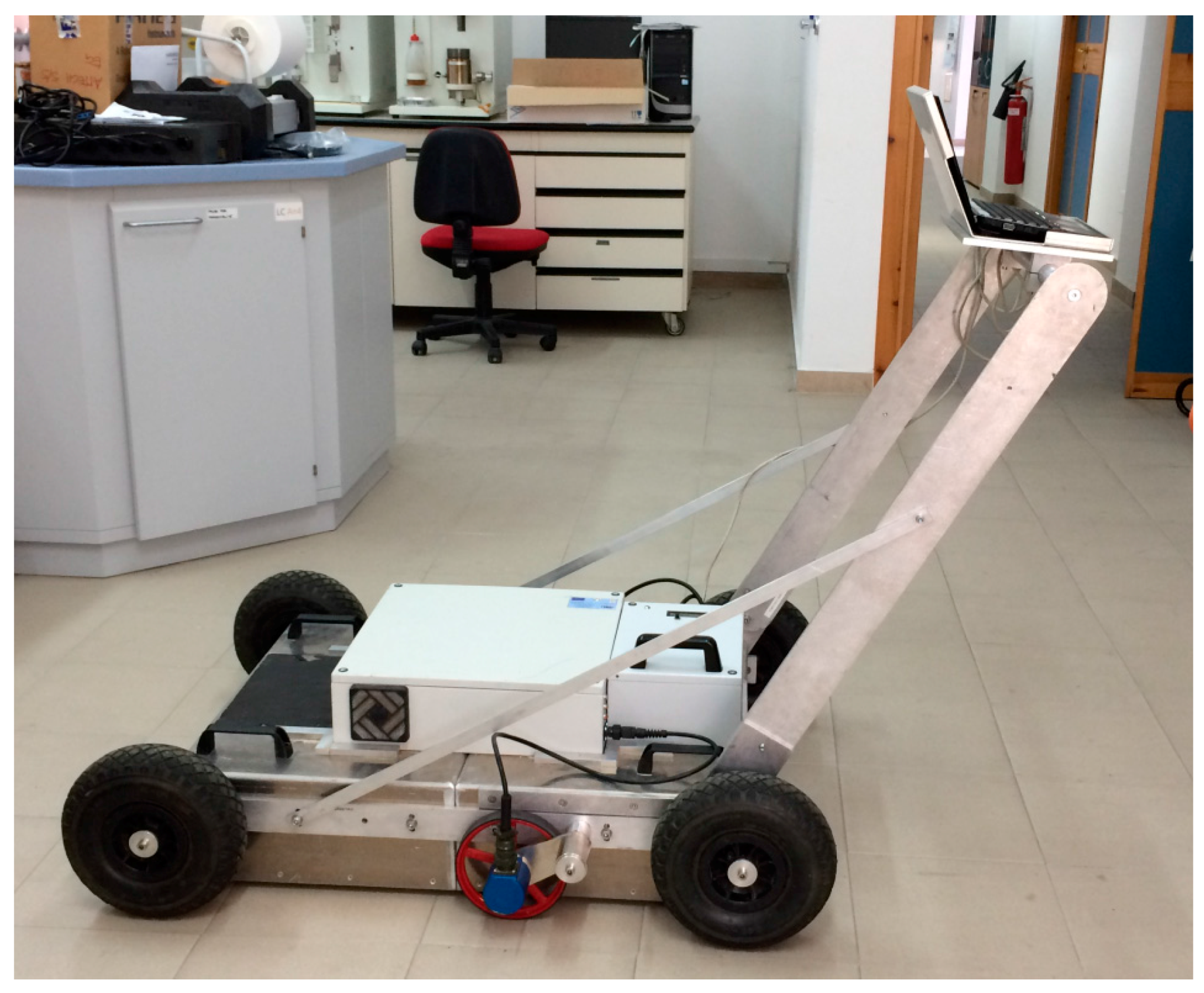
In this section we provide a brief description of the reconfigurable system. The system is shown in
Figure 1. It was implemented in 2010–2011 thanks to a collaboration between the Institute for Archaeological and Monumental Heritage IBAM-CNR, the Florence Engineering s.r.l. and the Ingegneria dei Sistemi (IDS) Corporation, Pisa, Italy. The system allows reconfiguration vs. the frequency, the length of the arms of the antennas, the radiated power at each frequency, and the integration time of each harmonic tone.
The reconfiguration of the radiated power is achieved with an attenuation selectively applicable on the frequencies. We have not yet tested it, but it may be useful in the case of some reflector that saturates the receiver only on some frequencies, for example.
The reconfiguration of the length of the arms of the antennas (essentially two bow-ties) has been achieved making use of two series of switches implemented with PIN diodes [
9].
This solution allowed implementation of three couples of equivalent antennas just by making the arms of a unique real couple of antennas longer or shorter, which of course saves space with respect to the case of three physically different couples of antennas. In particular, we might not know a-priori the depth of the targets of interest, and usually we do not know a-priori the characteristics of the soil. Consequently, we might not know a priori the optimal frequency band for the case history at hand, and so the possibility to simultaneously gather more Bscans with different bands can be helpful [
10,
11]. In particular, let us remark that several commercial systems contain a double couple of antennas, but to the best of our knowledge no one contains three couples of antennas together. The central frequencies of the three equivalent antennas of the reconfigurable system are placed at about 120, 250, and 550 MHz, with some site dependent variation, and the band of each equivalent antenna is of the same order of its central frequency. The system is able to sweep the band 50–1000 MHz (or part of it), with a frequency step optionally equal to 2.5 or 5 MHz.
Finally, as said, the system can reconfigure the integration time of the harmonic tones selectively, i.e., frequency by frequency. The integration time of the harmonic tones constitutes the parameter of interest in this paper. In particular, the possibility to selectively extend the integration times opens the problem of how to perform this extension in a proper way, which is the issue dealt with in the next section.
3. The Selective Extension of the Integration Time of the Harmonics
In this section, the algorithm implemented in order to reconfigure the integration time of the harmonic tones is described. In particular, the problem arises from the fact that the effects of the interferences depend not only on the level of the disturbing signals, but also on the sensitivity of the GPR system to these undesired signals, which in its turn depends on the shielding of the antennas (whose performance customarily depends on the frequency) and the strength of the useful signal, linked in its turn to the characteristics of the soil and to the depth and the characteristics of the targets. Therefore, the effects (if any) of the interferences are case dependent and have to be evaluated in situ from the available data. However, in general it is not easy to evaluate which frequencies are the most disturbed ones directly from the signal or from its spectrum, especially for large band interferences. In particular, it might become speculative to say that a peak of the amplitude spectrum (or some first kind discontinuity of the unwrapped phase spectrum) is a natural feature of the spectrum of the useful signal or is due to some interference, or both, especially if the phenomenon is not very pronounced. Incidentally, we have noticed that the derivative of the spectrum can provide some more reliable indication, because it can emphasize some of these features, but also in this case a meaningful degree of ambiguity remains. Rather, we have found that a parameter more suitable for the evaluation of the interference can be the variance of the gathered samples of signal at each frequency. In order to define this variance, let us outline that, in any stepped frequency system, the amplitude and phase of the received tone at the current frequency and in the current position is customarily retrieved by a heterodyne (more rarely a homodyne) demodulation receiving chain [
12]. This corresponds to retrieve the in-phase and quadrature components of the signal. In particular, at each position and sequentially for each frequency, the system transmits a tone that, with no loss of generality, we can express as
, and receives a tone with smaller amplitude and different phase, that we can express as:
From Equation (1) the in-phase component
I and the quadrature component
Q are defined as
Moreover, in order to average possible errors, customarily, any stepped frequency system does not gather just one in-phase and quadrature sample for each frequency, but rather N samples. N is chosen by the manufacturer, as well as the default duration of the integration times (in the case of the reconfigurable prototypal system, N = 63 and the default integration time is equal to 100 μs).
So, in the end the in-phase and quadrature gathered components are the algebraic averages of the
N gathered samples for each of the two quantities, respectively, equal to
The algorithm for the reconfiguration of the integration times exploits the variance of the
N stored samples of the in-phase and quadrature components, that we evaluate as:
In other words, lacking for a larger set of information that might allow some more refined statistical sampling [
13], we evaluate the variance identifying the statistical average of
I and
Q and of their squares with the algebraic average of their gathered samples. As outlined before, the variance evaluated in Equation (4) is calculated for a single frequency and a single trace. So, comprehensively—i.e., within a chosen calibration Bscan—
and
are two matrixes whose elements are indexed after the position and the frequency. We define therefore the Matrix of the Interferences
MI as follows:
being
the
k-th tone along the frequency sweep and
the
h-th trace along the Bscan. Then, we define the Vector of the Interferences
VI as follows:
VI is a vector depending only on the frequency, since we have maximized with respect to the position index. In other words, we account for the maximum interference at the current frequency wherever it occurs along the Bscan.
VI is a reasonable quantity for evaluating the effect of the interference (more in general, let say the “disturbance” composed by noise plus interference), because, in absence of any disturbing signal, the I and Q samples relative to the same tone should be equal to each other, which amounts to a null vector of interference: the differences within the I samples and within the Q samples are generated by noise and interferences, and the stronger the disturbing signals with respect to the useful signal are, the higher the variances of the I and Q samples are.
A question about the optimality of the path of the calibration Bscan remains unsolved. We do not have an answer for this question, which is also case dependent, but we can heuristically advise updating the vector of interference for very large areas, let us say with an interline step for this updating of 50 or 100 m. Let us also outline that we can exploit as calibration Bscan for the reconfiguration of the integration times just some of the Bscans of interest for the prospection at hand. In other words, customarily there is no need to spend extra time for gathering some calibration Bscans apart from the work being performed: just a little extra-time is required in order to check the value of the Vector of Interference for one or (for very large areas) a few among these Bscans.
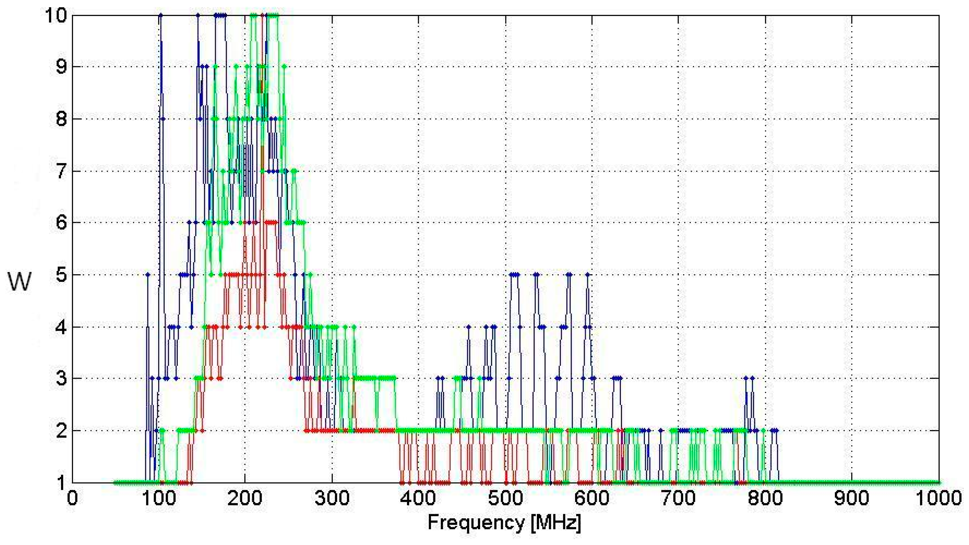
That said, the human operator can decide, on the basis of the radargram and of the Vector of Interference, whether some reconfiguration of the integration time of the harmonic tones is worth applying in the case at hand. If a reconfiguration is deemed worth applying, then the human operator has just to choose an integer number
M not smaller than 1, that somehow quantifies the “degree” of reconfiguration that he/she wants to implement. After setting this parameter, the reconfiguration code that we have implemented (in a MATLAB environment) sets a factor of enlargement for each integration time according to the following law:
being the factor of enlargement for the k-th tone and being Ceil the minimum integer not smaller than the argument. In particular, labeling as the default integration time of the instrument (that is the same for all the tones), after the reconfiguration the k-th tone will have a duration equal to , which is an integer multiple of , never shorter than (the Ceil function guarantees that) and never longer than whatever the choice of is. This saturation is due to that fact that the reconfigurable system does not allow to extend a tone more than 10 times its default value. If , the effect of the reconfiguration is to extend 10 times the integration time of the most disturbed tone and about proportionally less the other tones. If we choose , there might be several tones extended 10 times their default value.
Indeed, since the system is equipped with three couples of equivalent antennas, we have to set a value of for each of them. In fact, the interference possibly suffered by an antenna can be meaningfully different from that suffered by another one. It can also happen that the reconfiguration of the integration times is well advised for a couple of antennas and is not needed at all for another one. In this case, the operator can set (from which it follows ) for the “non-disturbed” antennas.
However, there is a last problem to be reported and to be account for: At the moment the acquisition software is not able to read three different integration time reconfiguration files (one for each equivalent couple of antennas), but only one. Therefore, after calculating three reconfiguration files, the current integration time reconfiguration code extracts from them a unique final file retaining for each frequency the maximum extension factor retrieved among the three antennas. This results in an extra-extension of the time needed for each measurement, in general not critical for narrow band interferences but possibly more relevant for large band interferences.
4. Experimental Test
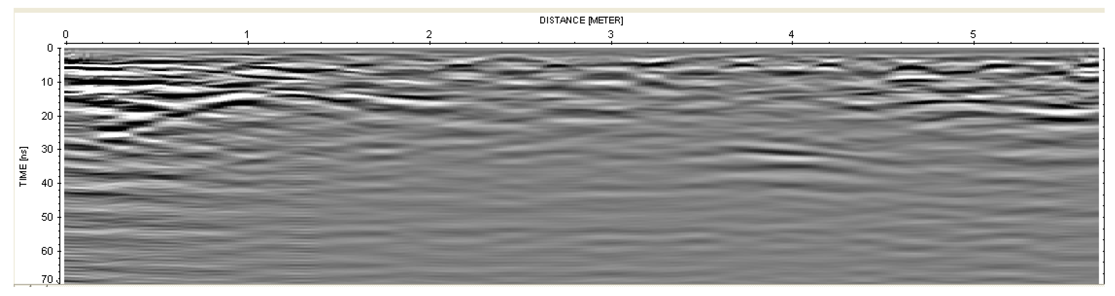
An experimental test has been performed in the corridor of the ground floor of the Institute for Archaeological and Monumental Heritage IBAM-CNR, in Lecce, Italy. In order to generate a large band interference, a second GPR system has been exploited, namely a pulsed Ris-Hi mode manufactured by IDS Corporation, equipped with two pairs of antennas with nominal central frequencies at 200 and 600 MHz, respectively. The pulsed GPR was taken still but continuously radiating, whereas the reconfigurable GPR system was passed by it along the gathered Bscan.
We repeated the measure three times, the first time with the pulsed GPR switched off and the stepped frequency set with its default integration times, the second time with the pulsed GPR switched on and with the stepped frequency set again with its default integration times (this second Bscan was exploited in order to evaluate the Vector of Interferences exploited for the reconfiguration of the integration times for the third Bscan), the third time with the pulsed GPR switched on and with the stepped frequency system set with reconfigured integration times.
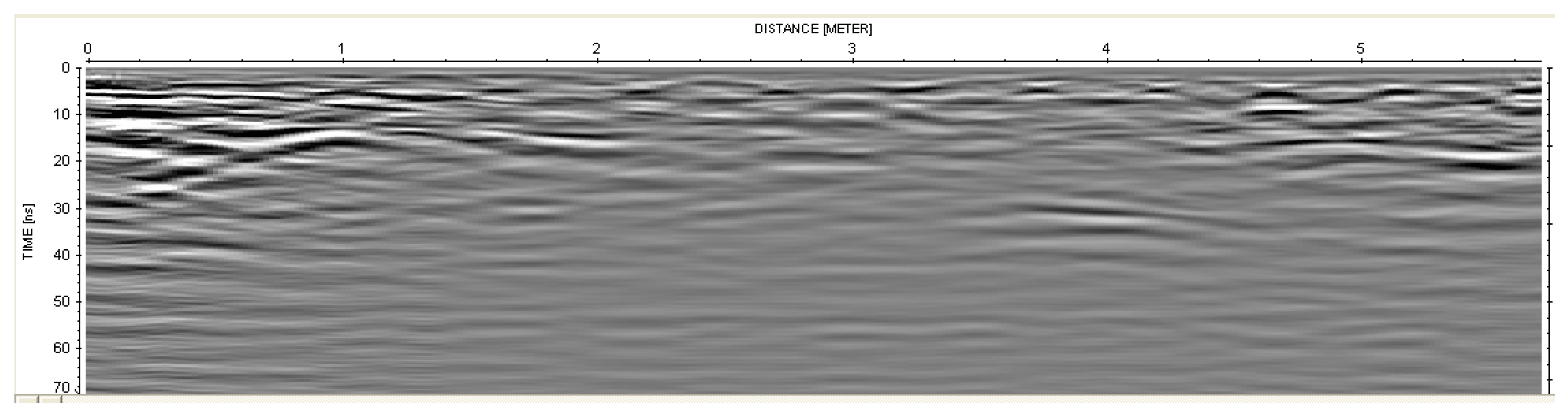
The first Bscan, achieved with the pulsed GPR switched off, is shown in
Figure 2. The data in
Figure 2 have been processed with the Reflexw commercial code [
14] according to a sequence processing composed by zero timing, background removal, gain vs. depth, one dimensional filtering, and Kirchoff migration. The propagation velocity has been evaluated equal to 0.08 m/ns according not only to the diffraction hyperbolas [
15] but also according to a sequential migration [
16] based on heuristic trials and visualizations of the relative results [
17].
From the data, a two-layer structure of the soil is evident, and we have reasons to suspect also some horizontal variation of the characteristics of the soil. This is coherent with some available a priori information, namely the fact that the building was enlarged with respect to its original size, and the bound between the “old” part and the “new” one is at about the abscissa 1 m in
Figure 2. In particular, under the newer part of the corridor, the periodic elements of a welded steel mesh are visible too. The data refer to the shortest equivalent antennas, because they provide the best resolution.
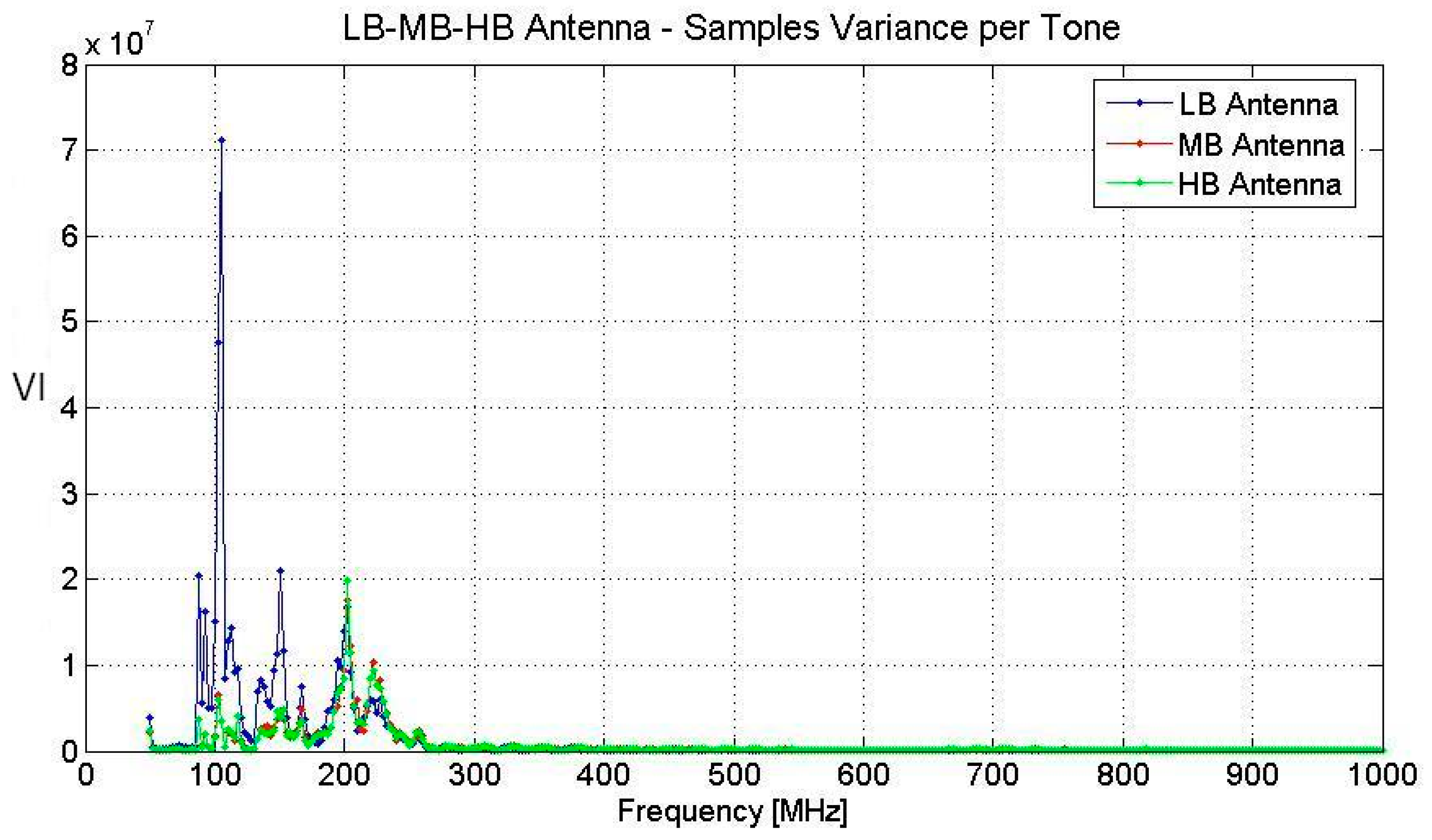
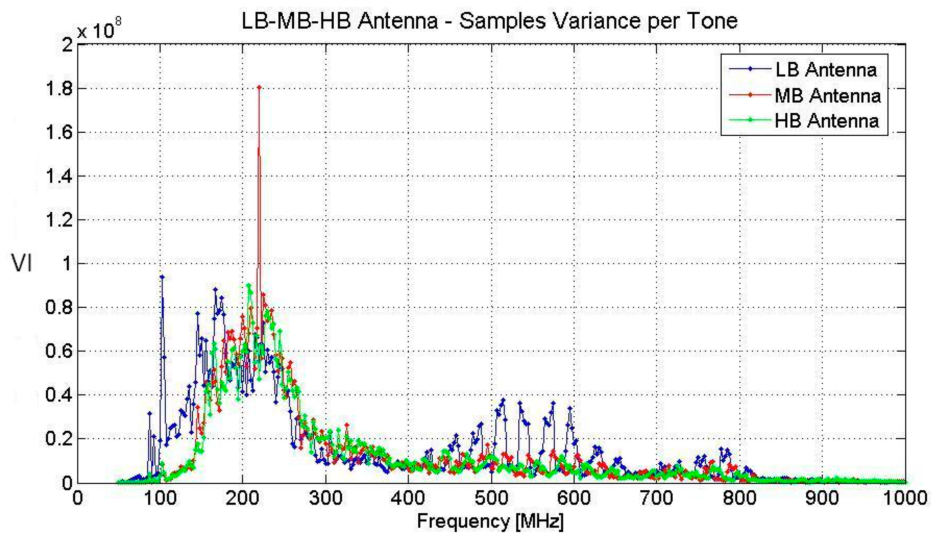
In
Figure 3 the Vector of Interferences is shown.
Figure 3 shows three graphs, one for each equivalent antenna of the reconfigurable GPR. From
Figure 3, we see that the stronger peak of the Vector of the Interferences is at about 100 MHz. This is quite probably due to the FM broadcast radio transmissions, that in Italy have their reserved bands in the range 88–110 MHz. However, some other sources of interference are also perceived, with peaks at about 150, 200, and 220 MHz.
In the case at hand, the interferences do not appear to be particularly critical, because they do not produce any meaningful “plot” effect or any “rain” effect, that are the main evidence of interference described in the literature [
1,
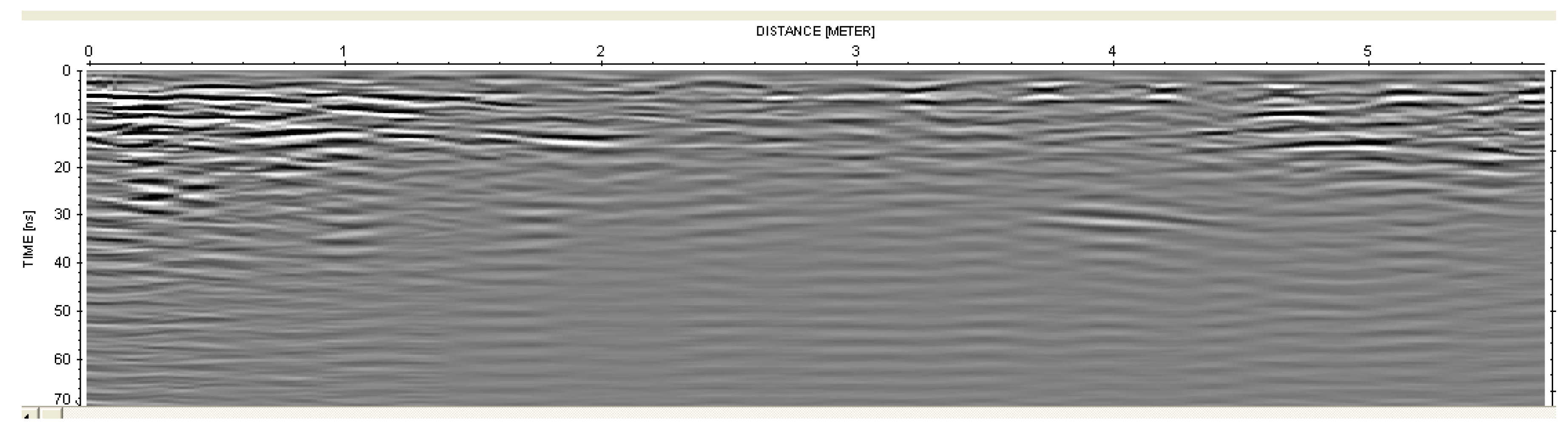
7]. Let us specify that we have not exploited this Vector of Interference for the reconfiguration of the integration times: we have shown it in order to allow a comparison with the case when the pulsed GPR is switched on. In fact, after this first measurement, the same observation line was travelled a second time with the pulsed GPR switched on. In this case, we achieved the result shown in
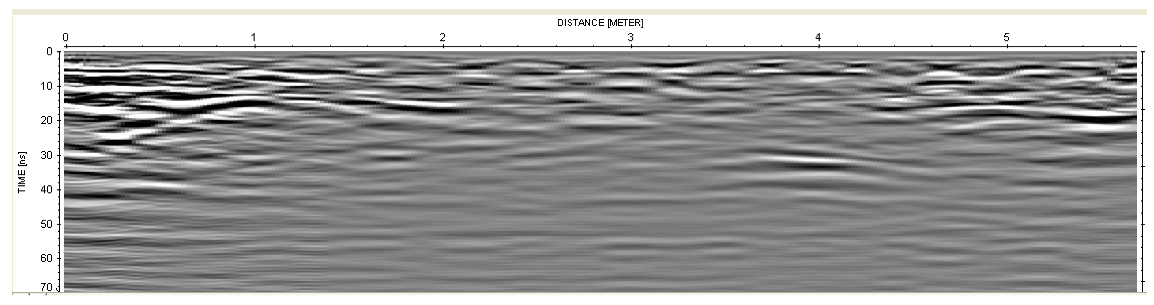
Figure 4.
The processing of the data was the same as that reported with regard to
Figure 2. From
Figure 4 we can appreciate a particular effect of the interference in the case at hand, namely a sort of inversion of the polarity of the buried anomalies, that appear to be substantially the same, but with the vertical “white-black” sequences replaced by “black-white” sequences and vice-versa. We are not able to explain the physical reasons of this inversion of polarity but it necessarily is an effect of the interference because no other condition was changed from the first to the second measure (the measurements were also repeated in two different moments, and this effect was confirmed). Whether such an effect is important or not depends on the application. In some cases, it is of interest to infer the nature of the buried targets from the polarity of the reflection [
18], and so an inversion of this polarity can be tricky with regard to the interpretation of the results. The Vector of the Interferences with the pulsed GPR switched on is shown in
Figure 5. As can be seen, switching on the pulsed GPR amounted in an increase of both the average level and the band of the interference. In particular, the band of the interferences appears centered around about 200 MHz.
This is likely to be ascribable to a better shielding of the antennas of the prototypal stepped frequency system at higher frequencies. On the basis of the achieved results we decided to apply a reconfiguration of the integration times, choosing
M = 12 for each of the three antennas. This amounted to a comprehensive extension of the time needed for the entire frequency sweep (from 50 MHz to 1000 MHz with frequency step 2.5 MHz) times a factor 2.41, which is meaningful but is in any case quite smaller than 10 (that is the maximum extension available for each harmonic signal). The calculated extension factors vs. frequency are shown in
Figure 6. At this point, we gathered again the data along the same observation line. However, we applied a reconfiguration of the integration times according to the set parameters and we achieved the data shown in
Figure 7. As can be seen, the polarity of the anomalies now is again the same as it was with the pulsed GPR switched off.
We clocked the time needed for gathering the Bscan, and it was about 36 s with a velocity of the order of one-half of that impressed to the stepped frequency system when the pulsed one was switched off. We repeated the experiment, and we have to report that, without this slowing of the human operator, the signal showed an evident loss of resolution.
5. Discussion
It is not immediate to compare the results presented in this paper with those present in literature because the GPR system exploited for the hardware rejection of the interference is, as said, a prototype, and at the moment we do not know of any other reconfigurable GPR system available on the market. So, other prospecting performed with a reconfigurable system do not exist to our knowledge. Indeed in the literature is present a meaningful number of studies on reconfigurable antennas, but they are performed in the field of the telecommunications systems, and in this framework the reconfigurability is meant as the possibility to change the direction of the main beam of an array of antennas, or to switch the exploited band of frequencies in order to counteract a possible atmospheric fading [
19]. The prototype exploited for the present contribution somehow translates the concept of reconfigurability into the context of the GPR prospecting.
Said that, if a meaningful interference is recognized or at least “strongly suspected” in the data gathered with a conventional GPR system, the commonly adopted praxis [
1] is to filter the data so that the “interferenced” band is at least partially rejected. So, for comparison with the state of art, we now propose the result of a filtering applied on the data relative to
Figure 4, i.e., the data achieved with the pulsed GPR switched on and with the stepped frequency GPR system working with its default integration times. On the basis of
Figure 5, we have filtered the result accounting for the band (at −3 dB) of the Vector of Interferences. This amounted to applying a Butterworth filter with lower cut-off frequency at 250 MHz and upper cut-off frequency at 1000 MHz. The achieved result is shown in
Figure 8. As can be seen, the polarity of the anomalies in many cases comes back to the same as that achieved without the interference of the pulsed system (see
Figure 2), but there is an evident drawback in terms of details present in the image. In particular, some anomalies are weakened or almost erased with respect to
Figure 2 and
Figure 4.
On the other side, as already outlined, the integration time reconfiguration involves, as a drawback, an extension of the time needed for the frequency sweep after reconfiguration, which involves, in its turn, the necessity to make slower the velocity of the human operator, at least for large band interferences. So, the question about whether it is convenient and practicable to apply the reconfiguration is case dependent: here we have shown it as a possibility.
6. Conclusions
In this paper, we have shown a possible effect of a large band interference on GPR data and a possible mitigation of this interference by means of a programmed modulation of the integration times of the harmonic tones radiated by a stepped frequency system.
To this, it is worth considering the fact that other situations, beyond the “artificial” case presented here, might make a large band interference more meaningful and harmful than shown here. Such a situation might exist, for example in some military or militarized context (where the interference might be created on purpose for several strategic reasons), or the problem might be particularly relevant in relationship with high frequency antennas. In fact, high frequency GPR antennas (e.g., antennas with a central frequency at 2 or 4 GHz) can be exploited for prospecting on walls, and in some case (especially for thin walls), some interferences might come from the external environment beyond the wall, in which case it is not mitigated at all by the shielding of the GPR antennas.
Future work will be devoted to reducing the inefficiencies of the reconfiguration code reported before in this paper, and another source of inefficiency (common to any current stepped frequency system to our knowledge) is the fact that the default integration time is the same at any frequency (it would be probably more efficient to set the same number of periods for the integration of any tone). Moreover, for the exploited prototype the default integration time is quite long. We know that commercial stepped frequency systems customarily adopt a shorter default integration time.


