Article

Hyperspectral Reflectance Anisotropy Measurements Using a Pushbroom Spectrometer on an Unmanned Aerial Vehicle—Results for Barley, Winter Wheat, and Potato

Laboratory of Geo-Information Science and Remote Sensing, Wageningen University & Research, Droevendaalsesteeg 3, 6708 PB Wageningen, The Netherlands
*
Author to whom correspondence should be addressed.
Remote Sens. 2016, 8(11), 909; https://doi.org/10.3390/rs8110909
Submission received: 26 September 2016 / Revised: 21 October 2016 / Accepted: 27 October 2016 / Published: 2 November 2016

Abstract

:
Reflectance anisotropy is a signal that contains information on the optical and structural properties of a surface and can be studied by performing multi-angular reflectance measurements that are often done using cumbersome goniometric measurements. In this paper we describe an innovative and fast method where we use a hyperspectral pushbroom spectrometer mounted on a multirotor unmanned aerial vehicle (UAV) to perform such multi-angular measurements. By hovering the UAV above a surface while rotating it around its vertical axis, we were able to sample the reflectance anisotropy within the field of view of the spectrometer, covering all view azimuth directions up to a 30° view zenith angle. We used this method to study the reflectance anisotropy of barley, potato, and winter wheat at different growth stages. The reflectance anisotropy patterns of the crops were interpreted by analysis of the parameters obtained by fitting of the Rahman-Pinty-Verstraete (RPV) model at a 5-nm interval in the 450–915 nm range. To demonstrate the results of our method, we firstly present measurements of barley and winter wheat at two different growth stages. On the first measuring day, barley and winter wheat had structurally comparable canopies and displayed similar anisotropic reflectance patterns. On the second measuring day the anisotropy of crops differed significantly due to the crop-specific development of grain heads in the top layer of their canopies. Secondly, we show how the anisotropy is reduced for a potato canopy when it grows from an open row structure to a closed canopy. In this case, especially the backward scattering intensity was strongly diminished due to the decrease in shadowing effects that were caused by the potato rows that were still present on the first measuring day. The results of this study indicate that the presented method is capable of retrieving anisotropic reflectance characteristics of vegetation canopies and that it is a feasible alternative for field goniometer measurements.

Graphical Abstract

1. Introduction

Natural surfaces reflect light anisotropically, which means that the reflected radiance varies with viewing and illumination geometry. Reflectance anisotropy is described by the bidirectional reflectance distribution function (BRDF), which is a function that quantifies the surface reflectance into a specific direction when being illuminated from a particular direction [1]. For remote sensing purposes, information on the BRDF is important, for example, for the correction of viewing and illumination effects [2] or for the calculation of albedo [3,4]. In addition to this, the BRDF has been shown to contain additional information on vegetation parameters, such as canopy density, foliar water content, nitrogen content and leaf area index [5], canopy height [6], canopy clumping [7,8] and soil properties, such as soil surface roughness [9] and soil moisture content [10]. Moreover, BRDF information can be used to improve classification accuracies [11].
Reflectance anisotropy is commonly studied by performing multi-angular reflectance measurements using goniometers in laboratories under controlled conditions e.g., [12,13,14,15] or in the field under natural conditions e.g., [16,17,18,19,20,21]. Both laboratory and field goniometer measurements have their advantages and disadvantages [22]. A drawback of using laboratory goniometry is that the observed target has to be taken out of its natural environment and that an artificial light source has to be used, which typically results in a non-parallel light beam as opposed to the natural illumination of the sun [23]. A positive aspect, on the other hand, is the full control over the position and stability of the light source during measurement acquisition. An advantage of field goniometry is that the target can be observed in its natural environment and under natural illumination conditions. However, this also has as a consequence that measurements are affected by influences of atmospheric conditions, wind, and changes in illumination conditions due to the movement of the sun and clouds [24]. A drawback of both laboratory and field goniometer measurements is that they are cumbersome and time consuming.
Unmanned aerial vehicles (UAVs) might provide more elegant opportunities for performing multi-angular reflectance measurements. The fast emergence and development of unmanned aerial platforms and lightweight optical sensors has recently boosted the availability of new techniques for acquiring spectral data [25]. The relatively low operation height of UAVs results in derived products with a small spatial pixel size [26], which are typically interesting for small scale precision agriculture applications [27,28,29]. UAVs have already become common platforms for use in remote sensing [30], but the number of studies that use UAVs to perform multi-angular measurements for investigation of reflectance anisotropy is still small.
Until now, only a few approaches of using a UAV to capture reflectance anisotropy have been explored. Hakala et al. [31] used a consumer camera mounted on a UAV to acquire reflectance anisotropy of snow-covered land surfaces and compared these with simultaneous ground measurements. Grenzdörffer and Niemeyer [32] also used a consumer-grade camera mounted on a UAV to study the anisotropic reflectance behavior of winter wheat fields by capturing images at different view zenith and azimuth angles covering the full hemisphere. Burkart et al. [33] used a hyperspectral UAV-based point spectrometer to collect multi-angular data of several vegetated areas and compared the measurements with the SCOPE model. Honkavaara et al. [34] have demonstrated a method for extracting the reflectance anisotropy from multi/hyperspectral frame images in the georectification process. Duan et al. [35] collected hyperspectral images of several crop types during two consecutive flights performed in different directions using a UAV, which resulted in pixels that were observed from two directions in the overlapping part of the two flight lines. Based on this dual angle dataset Duan et al. showed an improvement in the estimation of the leaf area index (LAI). Reflectance anisotropy is also reported as an unwanted effect: Rasmussen et al. [36] investigated the performance of different vegetation indices using a consumer-grade camera mounted on a UAV and observed strong angular variation in reflectance images acquired in sunny conditions. To avoid these anisotropic effects, they advised to acquire data during clouded days. Not only viewing geometry, but also illumination geometry, can have an influence on anisotropic reflectance effects. Brede et al. [37] studied the effect of solar zenith angle on the enhanced vegetation index (EVI) and found a linear trend in the decrease of the EVI with an increasing illumination zenith angle.
In this paper we present an innovative method to rapidly measure reflectance anisotropy using a UAV and a hyperspectral pushbroom spectrometer system. We demonstrate the method by two showcases: (1) we compare anisotropy measurements of barley and winter wheat, two different crops that are structurally comparable due to their vertically-oriented canopies. In addition, we show how differences in grain head development of both crops result in different anisotropy patterns; and (2) we show the effect of canopy development on reflectance anisotropy for potato crops by measurements before and after the potato canopy closed.

2. Materials and Methods

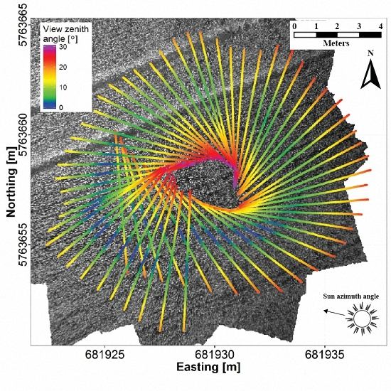
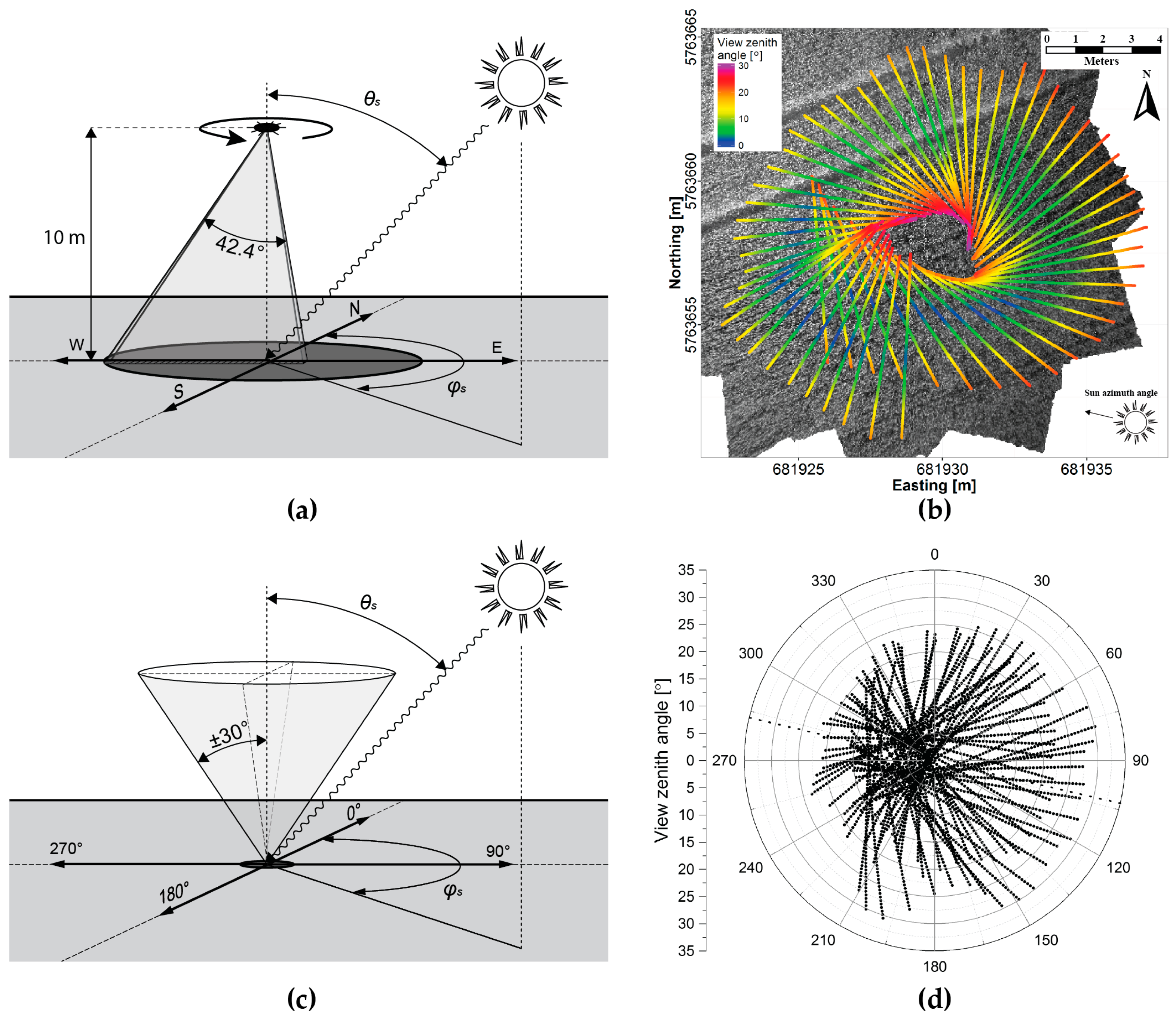
2.1. Study Area and Flight Pattern

The study area consisted of three fields with different crops located north of Wageningen, the Netherlands (51°59′34.8″N, 5°39′4.6″E). The study area was characterized as an open and flat agricultural area without any vertical elements nearby. The target crops were barley (Hordeum vulgare L., sowing date: 18 March 2015), potato (Solanum tuberosum L., sowing date: 14 April 2015), and winter wheat (Triticum aestivum L., sowing date: 21 October 2014), which were growing in three adjacent fields (Figure 1).
Several UAV flights were performed over the study area at two different growth stages of the crops during the summer of 2015 (Table 1). All measurements were taken under clear sky conditions to minimize the variance in diffuse illumination and to ensure the strongest directional effects.
The UAV measurements were performed using the Wageningen UR Hyperspectral Mapping System (HYMSY) on board an Altura AT8 octocopter [38], Figure 2. The HYMSY at its current configuration consists of a pushbroom spectrometer (450–915 nm, 9 nm full-width-at-half-maximum (FWHM), 25 lines/s, 328 pixels/line), a photogrammetric camera, and a miniature GPS-inertial navigation system (INS). The system and processing chain are specifically designed for agricultural mapping and monitoring applications of small areas (2–10 ha) in fine spatial detail.
The HYMSY is typically flown with the scanline of the spectrometer perpendicular to the flight direction and it produces a digital surface model (DSM) and a hyperspectral geocoded datacube, using orientations fused from the INS data and the photogrammetric orientation of the camera images. For the measurements of this study we took a different approach. Instead of performing the flight while maintaining the scanline of the spectrometer perpendicular to the flight direction, we flew the UAV while rotating it around its vertical axis at a constant rotation speed of approximately one revolution in 10 s. In this way, the azimuth orientation of each collected scanline was in a different azimuth plane. Based on the INS data and the photogrammetric orientation of the aerial images we derived the observation azimuth and zenith angles for each pixel. Collecting scanlines while completing full rotations with the UAV resulted in datasets covering the full 360° azimuth sampling range. While most goniometers sample the same area from multiple observation directions, the method presented in this paper takes multiple pixels in a sampling area from multiple observation directions. The rationale behind this is that, if the sampling area contains only a single crop or vegetation type and a large amount of pixels are measured, the measurements of the individual pixels will represent the reflectance anisotropy of the sampling area. The measurement principle can be compared to tower-based multi-angular measurements where different azimuth and zenith angles are sampled by rotating a sensor at a fixed position above a surface, such as the case of the Automated Multiangular Spectro-radiometer for Estimation of Canopy reflectance (AMSPEC) series [39,40,41] or the Portable Apparatus for Rapid Acquisition of Bidirectional Observation of the Land and Atmosphere III (PARABOLA III) [42].
The field of view (FOV) of the spectrometer’s scanline that was used for the measurements was 42.4°. When rotating the UAV while the center of the FOV is aimed towards the nadir position, the maximum zenith sampling angle would be 21.2°. To increase the maximum zenith sampling angle, we mounted the spectrometer tilted under the UAV to capture pixels at greater zenith angles (Figure 3a). The actual maximum zenith angle sampling range depends on the roll, pitch and yaw of the UAV during the flights and is, therefore, slightly different for each scanline.
For the data collection, the UAV was programmed to hover for one minute at a height of approximately 10 meters above ground level at a waypoint that was selected in the center of each of the fields. Operating at this height resulted in a ground sampling distance of about 6 cm. Once the UAV completed a 360° rotation around its vertical axis, a theoretically circular sampling area of approximately 100 m2 was covered. However, the rotational instability of the UAV resulted in a rotation around the waypoint, forming a ring-shaped sampling area (Figure 3b). Transforming the measurement scheme of Figure 3a to a polar coordinate system results in an angular sampling range up to around 30° zenith covering all azimuth directions (Figure 3c). The scanlines of Figure 3b result in a coverage of azimuth and zenith angles as shown in Figure 3d. The final collected datasets per crop consisted of 230,000–350,000 pixels within each sampling area at 94 spectral bands, ranging from 450 to 915 nm. In the fields there were some tractor tracks (Figure 3b), which for some targets and view directions formed a significant part of the sampled area. These tracks were manually filtered out before processing of the data. For the barley and winter wheat targets the observed anisotropy patterns could, therefore, be assigned solely to the crops. For the potato crops on the first measuring day, the anisotropy pattern is a combination of the signal of the potato plant and the soil background due to the open row structure of the potato canopy at this time (Figure 1).

2.2. Data Processing

The radiometric and geometric processing of the UAV data was done using the standard HYMSY processing chain described in detail in [38]. In this processing chain, the radiances measured by the spectrometer were converted to reflectance factors using the empirical line method with a measurement of a 25 cm × 25 cm 25% grey Spectralon panel (LabSphere Inc., North Sutton, NH, USA) and a dark current measurement taken just prior to the flight. To improve the signal-to-noise ratio, we applied Gaussian smoothing with a FWHM of ±5 bands (±25 nm) to the spectra.
For the geometric alignment of the HYMSY, aerial photos collected during the flights were aligned in Agisoft PhotoScan software (v1.1.2, AgiSoft LLC, St. Petersburg, Russia). The photogrammetric alignment of the photos was then fused with the data from HYMSY GPS INS to calculate view zenith and azimuth angles of each pixel. In the standard HYMSY processing these geometric metadata would have been used for the georectification of the hyperspectral data but, for the reflectance anisotropy measurements presented here, this step was omitted.
Due to the low accuracy of the magnetic compass in the HYMSY system and the lack of horizontal movement during the flights to exploit GPS data for sensor headings, the accuracy of azimuth angles retrieved from the standard HYMSY processing was found to be inadequate. Therefore, it was still mandatory to manually define the solar principal plane in the reflectance anisotropy data and use that to define the view azimuth angles. The accuracy of the final azimuth and zenith angles was estimated to be better than 2°. Usage of ground control points in the experiment would have resulted in better angular accuracy and removed the need for manual correction.

2.3. Data Analysis

The reflectance anisotropy was quantified using the anisotropy factor (ANIF). The ANIF is a ratio that describes the reflectance factor relative to the nadir reflectance factor [15]:
A N I F ( λ , θ i , φ i , θ r , φ r ) = R ( λ , θ i , φ i , θ r , φ r ) R 0 ( λ , θ i , φ i , 0 ° , 0 ° )
where R is the reflectance factor at wavelength λ observed from direction [ θ r , φ r ] and illuminated from direction [ θ i , φ i ]. R 0 is the reflectance factor at the nadir view.
To smoothen and filter the measurements, the data were resampled to a discrete grid of 1° azimuth and zenith view angles. We applied an angular smoothing of an area of 5° radius around each discrete azimuth and zenith observation angle to be able to assign a single reflectance factor to an observation position. A discrete azimuth and zenith observation angle was only considered if there were at least 1000 pixels within this 5° radius.
To interpret the measurements and parameterize the anisotropy patterns, we fitted the Rahman-Pinty-Verstraete model (RPV) [43] through each dataset. The RPV model is a semi-empirical model that uses four parameters to simulate the BRDF of any arbitrary surface. It has been used in anisotropy studies of a wide variety of targets like forests [44], grasslands and cultivated fields [45], snow [31], and soil [10,46] at different scales ranging from the centimeter scale in laboratory studies [10,47], to the decimeter scale in UAV- and airborne-based studies [11,31], up to a scale of several hundreds of meters to a kilometer scale in space-borne studies. The model splits the reflectance anisotropy in an amplitude component ( ρ 0 ) and a directional component:
ρ s ( θ i , φ i ; θ r , φ r ) = ρ 0 c o s k 1   θ i   c o s k 1   θ r ( c o s θ i + c o s θ r ) 1 k F ( g ) [ 1 + R ( G ) ]
where the k parameter controls the bowl/bell shape of the anisotropy curve. The relative amount of forward/backward scattering, controlled by the Θ parameter, is defined as:
F ( g ) =   1   Θ 2 [ 1 +   Θ 2 2 Θ c o s ( π g ) ] 1.5
where
g = c o s   θ i c o s   θ r + s i n   θ i   s i n   θ r   cos ( φ i   φ r )
The hotspot is approximated by:
1 + R ( G ) = 1 +   1   ρ c 1 + G
where
G = [ t a n 2   θ i +   t a n 2   θ r 2   t a n   θ i   t a n   θ r   cos ( φ i   φ r ) ]   1 / 2
To estimate the parameters that best describe the anisotropy, the RPV model was fitted through the multi-angle reflectance measurements by a non-linear least squared regression method that uses the Levenberg-Marquardt algorithm, implemented in R (version 3.3.1) [48]. The range of possible solutions for the fitting of the RPV model for the Θ parameter was restricted between −1 and 1, where Θ <0 indicates predominant backward scattering and Θ >0 indicates predominant forward scattering anisotropy. Since no measurements were taken close to the hotspot (Table 1), the ρ c parameter was fixed at 1, which indicates no additional fitting around the hotspot position. The range of the k parameter was left free, where k <1 resembles a bowl-shaped anisotropy curve and k >1 resembles a bell-shaped anisotropy curve.

3. Results and Discussion

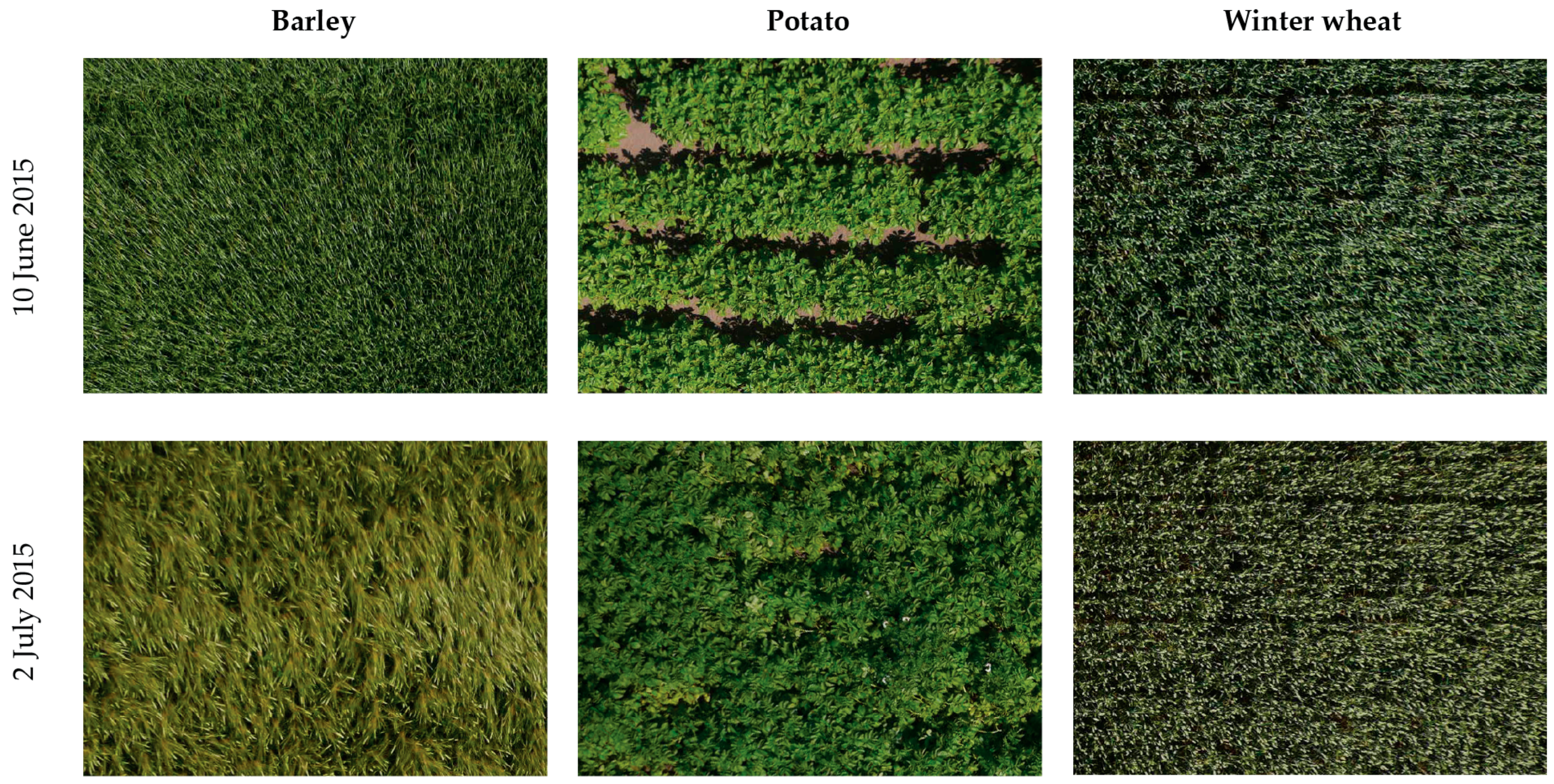
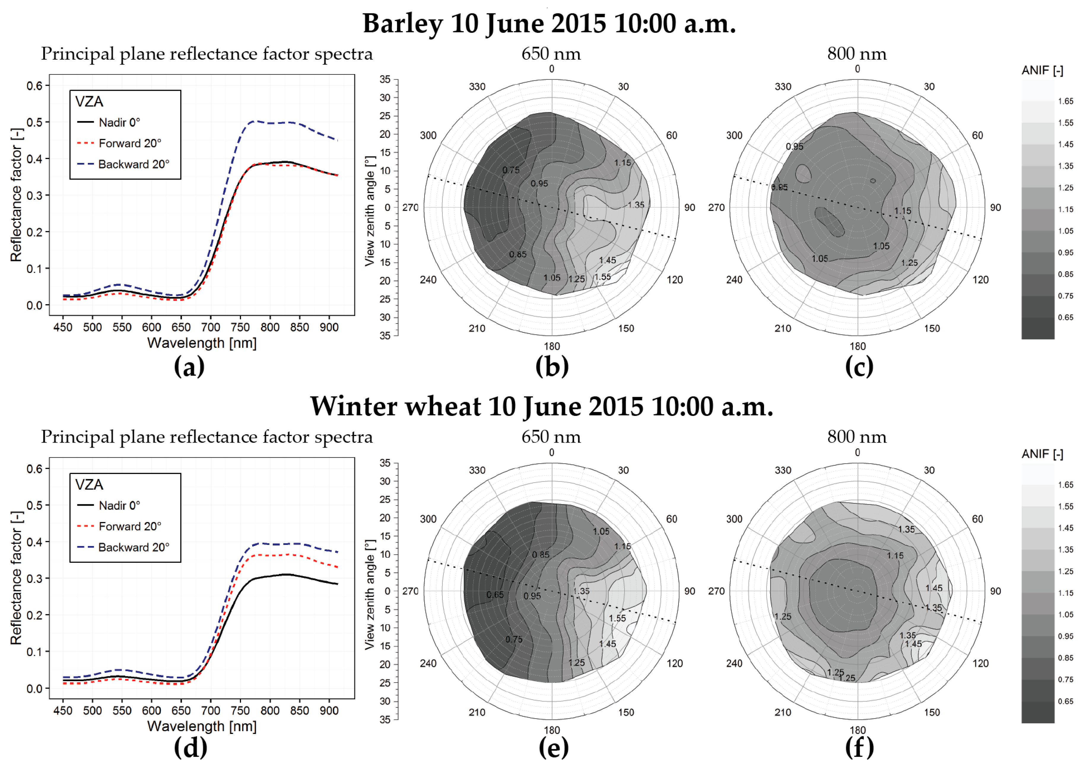
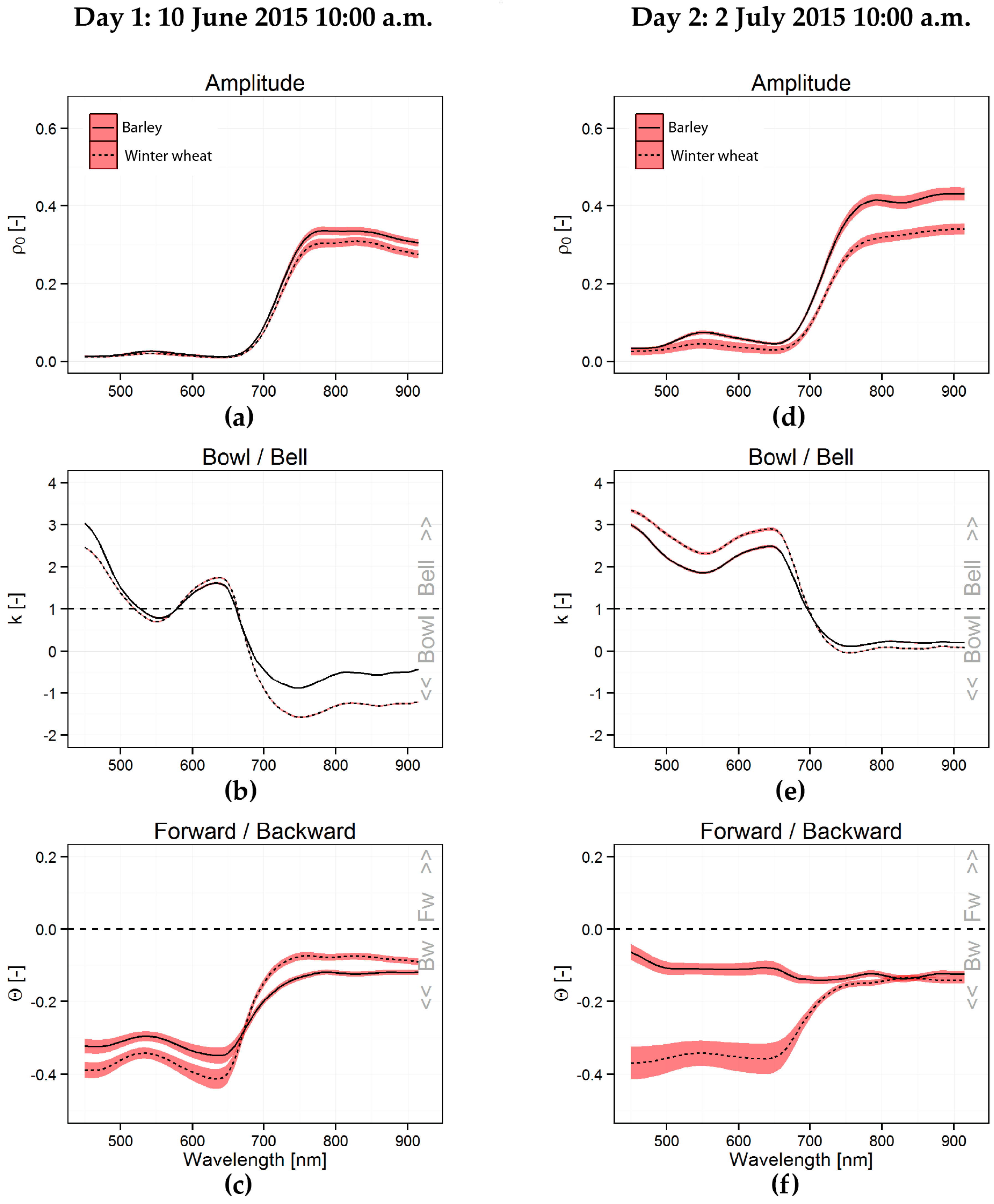
3.1. Barley and Winter Wheat

On the first measuring day, when the top layer of the barley and winter wheat canopies were still formed by leaves, both the barley and winter wheat displayed typical anisotropy characteristics, as are commonly seen for vertically-oriented canopies. In the red band (650 nm), where shadows are darkest due to absorption of radiance by chlorophyll, the lowest ANIFs were observed in the forward scattering direction and the highest ANIFs in the backward scattering direction (Figure 4b,e).
This effect occurs because, in the backward scattering direction, the sensor was viewing the well-illuminated side of the canopies, which resulted in a higher reflectance, and in the forward scattering direction the shadowed side of the canopies, which resulted in a lower reflectance. In addition to this effect, view zenith angles (VZAs) close to nadir allow for a view of the lower shadowed layers of the canopy and with increasing off-nadir VZAs the relative proportion of higher, well-illuminated canopy layers that are observed by the sensor increases, resulting in an increase of reflectance [15,49].
In the near-infrared band (NIR, 800 nm), where shadow effects are weaker due to lower absorption of radiance by chlorophyll, the ANIFs increased with increasing view zenith angles, independent of the view azimuth direction. The small contribution of the shadow effect puts the position of the lowest observed ANIF close to nadir, slightly in the forward direction (Figure 4c,f).
The k and Θ -parameter spectra, obtained at a 5-nm interval between 450 nm and 915 nm by fitting the RPV model through the measurements of flights 1 and 3 on day 1 and day 2 at 10:00 a.m. (Table 1), illustrate the observed anisotropy patterns in terms of the reflectance bowl/bell-shaped anisotropy and forward/backward scattering dominance, respectively (Figure 5a–c). On the first measuring day, both crops were in a pre-heading stage and the top layers of their canopies were mainly formed by leaves. For both crops at this stage, the k parameter spectrum followed a trend opposite to that of a vegetation reflectance factor spectrum (Figure 5b). The blue and red wavelengths had k >1, indicating a bell-shaped anisotropy curve. At these wavelengths the anisotropy was dominated by shadow effects due to the strong absorption of radiation by chlorophyll in the leaves that formed the top layer of the barley and winter wheat canopies. Accordingly, this resulted in the lowest values of Θ in these wavelength regions (Figure 5c). In the green part of the spectrum these shadow effects were weaker due to less absorption by chlorophyll in this region, resulting in slightly higher Θ values and k values just below 1. k values <1 were obtained by fitting the RPV model in the NIR wavelength region, indicating a bowl-shaped anisotropy pattern. Moreover, the backward scattering was weaker in this wavelength region, which resulted in Θ values of roughly −0.13 for barley and −0.09 for winter wheat between 750 and 915 nm (Figure 5c). Even though barley and winter wheat are different crops, both of them displayed very similar anisotropy patterns over the measured spectral domain on the first measurement day due to their similar canopy structures.
At the time of the second measuring day, both crops were in their grain development stage. This had as a result for barley that the top layer of the canopy was no longer formed by leaves, but by a layer of less photosynthetically active grain heads with large awns and the heads were clearly bending downwards (Figure 1). The anisotropy at this stage was characterized by an overall increased k parameter value at all measured wavelengths with k >1 in the visible wavelength region (Figure 5e). In addition, the backward scattering intensity decreased in the visible wavelengths with Θ values of around −0.33 to approximately −0.12 (Figure 5c,f).
The winter wheat canopy on the second measuring day was formed by vertically-oriented grain heads that were pointing out above the leaf layer, also resulting in less photosynthetically active material in the a top canopy layer. This resulted in a similar k spectrum as for the barley canopy (Figure 5e). The Θ parameter followed the same trend as during the first day, but with a less emphasized peak at green wavelengths. In the NIR wavelength region, the Θ parameter decreased from −0.09 to −0.16, indicating stronger shadow effects due to the presence of opaque grain heads in the top canopy layer.

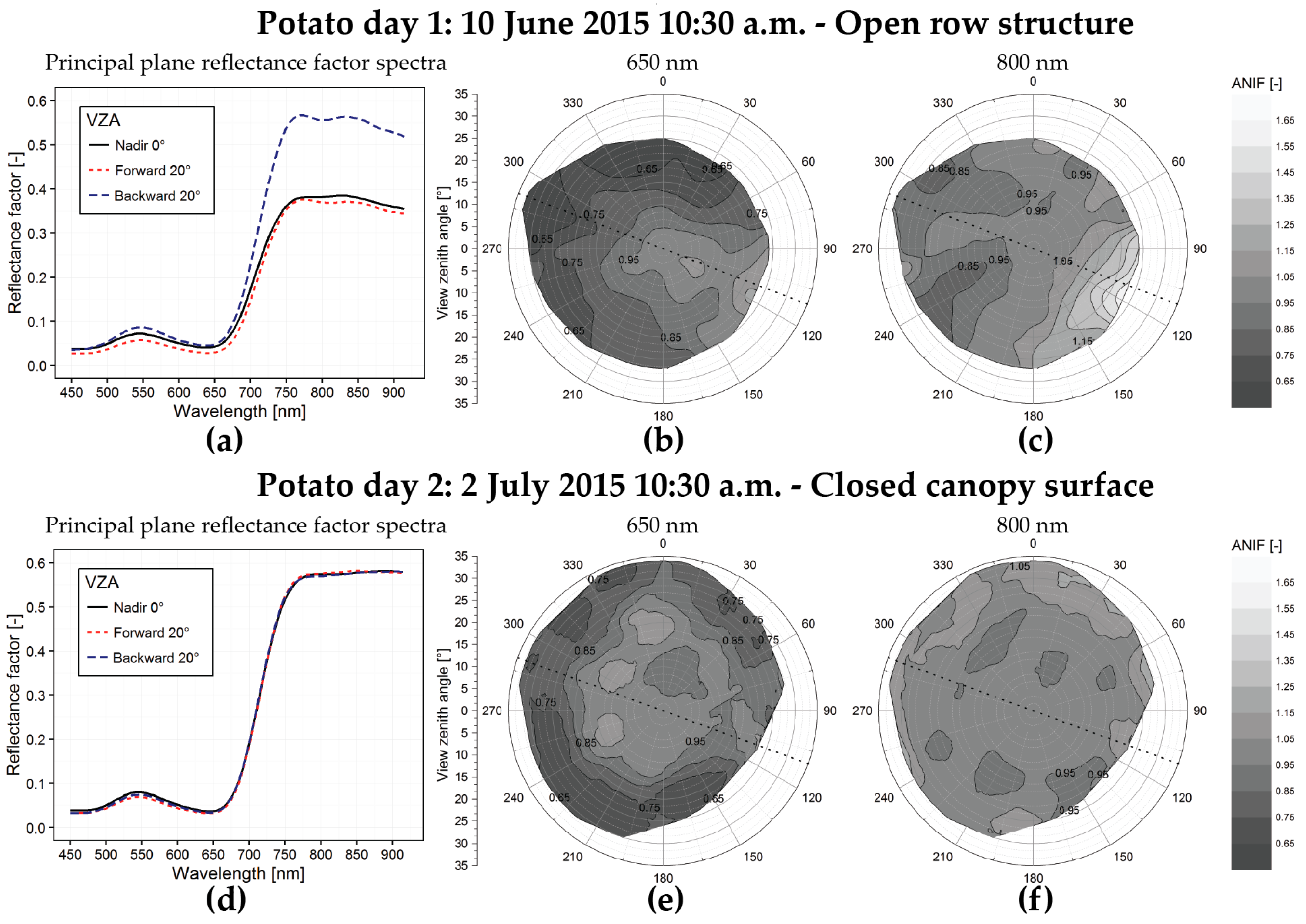
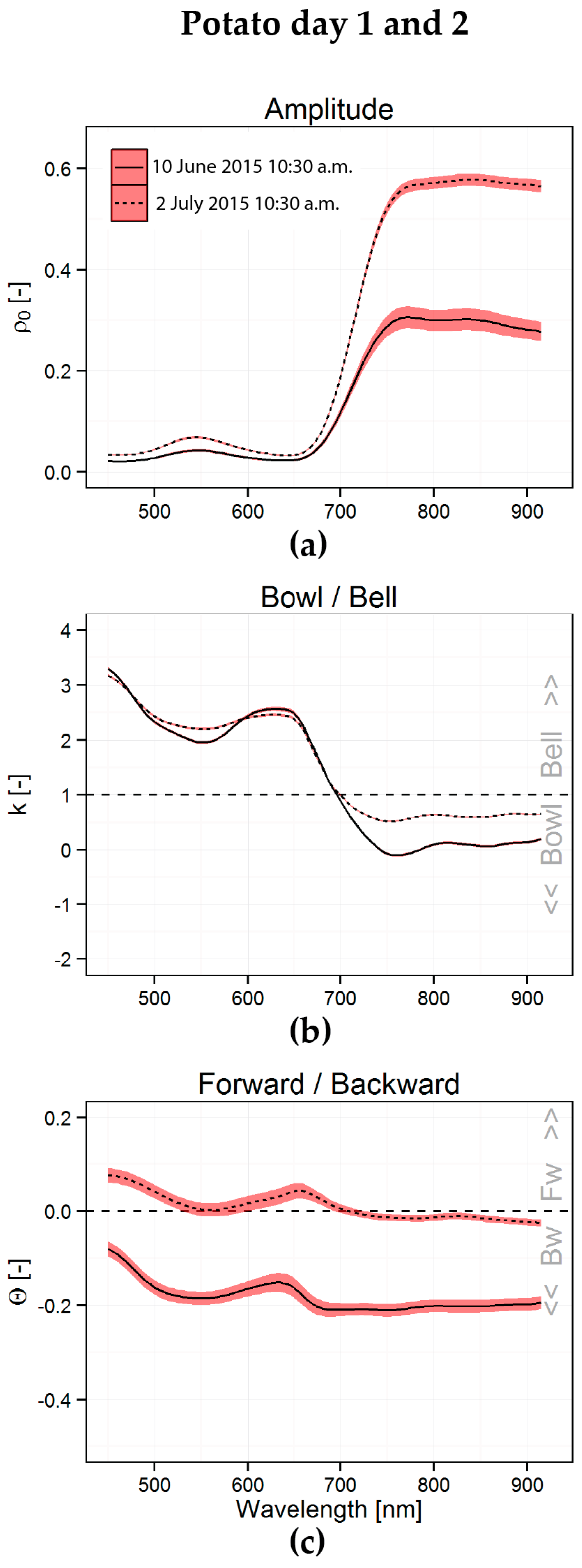
3.2. Potato Canopy Closure

On measurement day 1, when the potato canopy was showing an open row structure, the soil formed a significant part of the signal when measured by the sensor in the nadir view. With increasing VZA, the proportional area of observed soil decreased and the proportional area of observed vegetation increased. In the red wavelength region, an increase in VZA resulted, therefore, in a decrease of the reflectance factor, since soil has a higher reflectance at this wavelength compared to vegetation. In addition, the row structure of the potato crops produced strong shadows, which caused a higher reflectance in the backward scattering direction and lower reflectance in the forward scattering direction. This resulted in a bell-shaped curve with the highest ANIFs around the nadir and in the backward scattering direction (Figure 6b). Bell-shaped anisotropy curves are typically seen at bright surfaces that are partially covered by darker objects, such as sparse agricultural canopies [49] or snow-covered surfaces with snow-free trees [44]. In the NIR wavelength region an increase in VZA resulted in an increased ANIF, which is opposite to the red region, since vegetation has a higher reflectance in this wavelength region than soil.
Between measurement days 1 and 2, the potato canopy grew from an open row structure to a continuous surface covering the soil almost completely (Figure 1). In addition to a strong increase of the amplitude parameter in the NIR due to the increased vegetation cover (Figure 7a), this resulted in a significantly decreased reflectance anisotropy over the full measured wavelength region on day 2. Especially, we observed a strong decrease in backward scattering, which is clearly indicated by the increase of the Θ parameter to values close to 0 between day 1 and day 2 (Figure 7c).
The decrease in backward scattering is likely due to the disappearance of the open row structure between day 1 and day 2 and, thus, the absence of strong row-induced shadows. The general bowl/bell anisotropy pattern remained nearly the same between day 1 and 2, as can be seen by the similar k parameter spectra on both days (Figure 7b). However, the bowl shape was less pronounced in the 750–915 nm region as can be seen by the increase of the k values from around 0 to 0.58 on day 1 and 2, respectively. Likely, this happened because the less reflective soil in the NIR that was observed by the sensor on measurement day 1 at near nadir VZAs was no longer observed on day 2, resulting in a weaker increase of reflectance with increasing VZAs in this wavelength region.

3.3. General Discussion

We presented an innovative and fast method in which we captured reflectance anisotropy by extracting the multi-angular views that are collected by the HYMSY system. By hovering a UAV with a hyperspectral pushbroom spectrometer above a surface while rotating it around its vertical axis, we were able to obtain the reflectance anisotropy of several crops. As demonstrated, the described method can be used to rapidly acquire the reflectance anisotropy. It might be an interesting alternative to field goniometer measurements and is especially interesting for measurements of small canopies like those of agricultural crops.
The barley and winter wheat canopies on both measuring days and the potato canopy on the second measuring day were nearly completely covering the complete surface and, therefore, the anisotropy patterns that we observed for these targets can be attributed solely to the crops. The potato canopy on the first measuring day was not completely covering the surface. The observed anisotropy signal on this day was, thus, composed by both the potato plants and the exposed soil. The measurements of the potato crop on the first measuring illustrated how the row structure of the potato plants resulted in strong differences between forward and backward scattering due to the presence of shadows. The closing of the potato canopy resulted in an overall decrease of reflectance anisotropy, and especially in a decrease of backward scattering intensity, something that has also been observed with canopy closure of soybeans [50]. The anisotropy patterns of barley and winter wheat were dominated by backward scattering over the full measured spectral domain, with emphasis on the visible wavelength region, combined with a strong bell-shaped anisotropy in the NIR. Similar patterns for barley and wheat were also found in several other studies e.g., [51,52,53] and are typical for vertically-oriented vegetation canopies, such as grasses e.g., [14,15].
With our sensor hardware and additional tilt of the spectrometer, the maximum VZA was limited to 25°–35°, which matches the VZAs of most satellite and airborne remote sensing sensors. Very likely, extending the VZA to larger angles would provide more information on the reflectance anisotropy and would make the fitting of the RPV model, or any other BRDF model, more stable. Tilting the spectrometer at an even greater angle would result in sampling of larger VZAs. However, it has to be taken into account that a larger target surface is needed to make sure that the FOV of the sensor will stay within the target boundaries. The fields in our study area were quite narrow (±50 m) and to ensure that the sensor was only observing a single crop during the rotation of the UAV, we did not tilt the spectrometer any further, but we will experiment with extending the VZA in future measurements.
The strength of the presented method is the very high density of samples that are collected in a short amount of time. Since each of the pixels in the scanline of the spectrometer can be considered as an individual sample, this means that, per second, 328 × 25 = 8200 samples are collected at a 5-nm interval in the 450–915 nm range. By performing an angular smoothing as described in the methods section, the average anisotropy of a surface can be obtained, whereas most goniometers only provide the anisotropy of a single point, which does not have to be representative for the investigated target surface. Another strength of the data collected with our method is that it contains reflectance anisotropy at canopy level over the full spectrum. From the fitting of the RPV model, we can see that the changes in bowl/bell ( k ) and forward/backward ( Θ ) spectra mostly follow the changes of the normal reflectance factor spectrum. However, the relation does not seem to be linear, as sometimes small changes in nadir reflectance factor, for example in the green wavelength region, seem to produce disproportionally large changes in RPV parameters. The results indicate that the reflectance anisotropy signal contains information about the canopy beyond the extent of the basic (nadir) reflectance factor spectrum. Using our spectra it is also possible to evaluate the number of spectral bands necessary to generally describe the reflectance anisotropy of vegetation. Our RPV parameter spectra suggest that separate measurements in at least blue/UV, green, red, and a single NIR band should be sufficient to broadly describe the reflectance anisotropy of vegetation targets in the VIS-NIR range. Such a generic description of reflectance anisotropy should be sufficient for BRDF correction of imagery and generic algorithms extracting canopy structural parameters. For more advanced analysis of reflectance anisotropy, there still may be benefits in collecting full hyperspectral data. An interesting approach to reflectance anisotropy is to consider that from different view angles the observer detects different portions of the top-most and the deeper layers of the canopy [54]. In traditional remote sensing, it is possible to estimate leaf pigment concentrations in the canopy using hyperspectral data. Similarly, using hyperspectral anisotropy data, it might be possible to derive the distribution of pigments within the vertical structure of the canopy.

4. Conclusions

In this paper we presented a fast and innovative method to capture reflectance anisotropy using a pushbroom spectrometer mounted on a UAV as an alternative for cumbersome goniometer measurements. We used this method to collect the reflectance anisotropy of several agricultural crops at two different growth stages and fitted the RPV model to parameterize and interpret the measurements. Measurements of barley and winter wheat before heading showed very similar anisotropic reflectance patterns that were dominated by backward scattering ( Θ < 0) over the measured spectral domain (450–915 nm), with emphasis on the visible wavelengths, combined with a bowl-shaped anisotropy ( k < 1) in the NIR band for both crops. The development of grain heads on the second measurement day resulted in different composition of the top layers of the barley and winter wheat canopies, which resulted in distinctively different RPV parameter spectra for both crops, indicating a potentially useful signal of grain head development in the multi-angular reflectance observations. Measurements of potato showed a strong reduction of backscattering when the potato crops grew from an open row structure to a fully-developed canopy that was almost completely covering the surface. In our data the change in reflectance anisotropy was very distinct for all measured crops, suggesting that anisotropy effects could potentially be used as a signal in operational remote sensing.

Acknowledgments

This research was funded by a grant from the User Support Programme Space Research (GO/12-15) in The Netherlands. The authors would like to thank the Wageningen University & Research Unmanned Aerial Remote Sensing Facility (UARSF) for providing the UAV and sensor system used in this study.

Author Contributions

P.P.J.R. and J.M.S. conceived and designed the experiments; P.P.J.R. and J.M.S. performed the experiments; P.P.J.R. and J.M.S. analyzed the data; P.P.J.R., J.M.S., H.M.B., and J.G.P.W.C. contributed reagents/materials/analysis tools; P.P.J.R., J.M.S., H.M.B., and J.G.P.W.C. wrote the paper.

Conflicts of Interest

The authors declare no conflict of interest.

References

  1. Schaepman-Strub, G.; Schaepman, M.E.; Painter, T.H.; Dangel, S.; Martonchik, J.V. Reflectance quantities in optical remote sensing-definitions and case studies. Remote Sens. Environ. 2006, 103, 27–42. [Google Scholar] [CrossRef]
  2. Weyermann, J.; Damm, A.; Kneubuhler, M.; Schaepman, M.E. Correction of reflectance anisotropy effects of vegetation on airborne spectroscopy data and derived products. IEEE Trans. Geosci. Remote Sens. 2014, 52, 616–627. [Google Scholar] [CrossRef]
  3. Lucht, W.; Schaaf, C.B.; Strahler, A.H. An algorithm for the retrieval of albedo from space using semiempirical BRDF models. IEEE Trans. Geosci. Remote Sens. 2000, 38, 977–998. [Google Scholar] [CrossRef]
  4. Schaaf, C.B.; Gao, F.; Strahler, A.H.; Lucht, W.; Li, X.; Tsang, T.; Strugnell, N.C.; Zhang, X.; Jin, Y.; Muller, J.P.; et al. First operational BRDF, albedo nadir reflectance products from MODIS. Remote Sens. Environ. 2002, 83, 135–148. [Google Scholar] [CrossRef]
  5. Kneubühler, M.; Koetz, B.; Huber, S.; Schaepman, M.E.; Zimmermann, N.E. Space-based spectrodirectional measurements for the improved estimation of ecosystem variables. Can. J. Remote Sens. 2008, 34, 192–205. [Google Scholar]
  6. Wang, Y.; Li, G.; Ding, J.; Guo, Z.; Tang, S.; Wang, C.; Huang, Q.; Liu, R.; Chen, J.M. A combined GLAS and MODIS estimation of the global distribution of mean forest canopy height. Remote Sens. Environ. 2016, 174, 24–43. [Google Scholar] [CrossRef]
  7. Chen, J.M.; Menges, C.H.; Leblanc, S.G. Global mapping of foliage clumping index using multi-angular satellite data. Remote Sens. Environ. 2005, 97, 447–457. [Google Scholar] [CrossRef]
  8. He, L.; Chen, J.M.; Pisek, J.; Schaaf, C.B.; Strahler, A.H. Global clumping index map derived from the modis BRDF product. Remote Sens. Environ. 2012, 119, 118–130. [Google Scholar] [CrossRef]
  9. Wang, Z.; Coburn, C.A.; Ren, X.; Teillet, P.M. Effect of soil surface roughness and scene components on soil surface bidirectional reflectance factor. Can. J. Soil Sci. 2012, 92, 297–313. [Google Scholar] [CrossRef]
  10. Roosjen, P.P.J.; Bartholomeus, H.M.; Clevers, J.G.P.W. Effects of soil moisture content on reflectance anisotropy—laboratory goniometer measurements and RPV model inversions. Remote Sens. Environ. 2015, 170, 229–238. [Google Scholar] [CrossRef]
  11. Koukal, T.; Atzberger, C.; Schneider, W. Evaluation of semi-empirical BRDF models inverted against multi-angle data from a digital airborne frame camera for enhancing forest type classification. Remote Sens. Environ. 2014, 151, 27–43. [Google Scholar] [CrossRef]
  12. Biliouris, D.; Verstraeten, W.W.; Dutré, P.; Van Aardt, J.A.N.; Muys, B.; Coppin, P. A compact laboratory spectro-goniometer (ClabSpeG) to assess the BRDF of materials. Presentation, calibration and implementation on Fagus sylvatica L. Leaves. Sensors 2007, 7, 1846–1870. [Google Scholar] [CrossRef]
  13. Feingersh, T.; Ben-Dor, E.; Filin, S. Correction of reflectance anisotropy: A multi-sensor approach. Int. J. Remote Sens. 2010, 31, 49–74. [Google Scholar] [CrossRef]
  14. Roosjen, P.P.J.; Clevers, J.G.P.W.; Bartholomeus, H.M.; Schaepman, M.E.; Schaepman-Strub, G.; Jalink, H.; van der Schoor, R.; de Jong, A. A laboratory goniometer system for measuring reflectance and emittance anisotropy. Sensors 2012, 12, 17358–17371. [Google Scholar] [CrossRef] [PubMed] [Green Version]
  15. Sandmeier, S.; Müller, C.; Hosgood, B.; Andreoli, G. Physical mechanisms in hyperspectral BRDF data of grass and watercress. Remote Sens. Environ. 1998, 66, 222–233. [Google Scholar] [CrossRef]
  16. Bachmann, C.M.; Abelev, A.; Montes, M.J.; Philpot, W.; Gray, D.; Doctor, K.Z.; Fusina, R.A.; Mattis, G.; Chen, W.; Noble, S.D.; et al. Flexible field goniometer system: The goniometer for outdoor portable hyperspectral earth reflectance. J. Appl. Remote Sens. 2016, 10. [Google Scholar] [CrossRef]
  17. Coburn, C.A.; Peddle, D.R. A low-cost field and laboratory goniometer system for estimating hyperspectral bidirectional reflectance. Can. J. Remote Sens. 2006, 32, 244–253. [Google Scholar]
  18. Deering, D.W.; Leone, P. A sphere-scanning radiometer for rapid directional measurements of sky and ground radiance. Remote Sens. Environ. 1986, 19, 1–24. [Google Scholar] [CrossRef]
  19. Painter, T.H.; Paden, B.; Dozier, J. Automated spectro-goniometer: A spherical robot for the field measurement of the directional reflectance of snow. Rev. Sci. Instrum. 2003, 74, 5179–5188. [Google Scholar] [CrossRef]
  20. Sandmeier, S.R.; Itten, K.I. A field goniometer system (Figos) for acquisition of hyperspectral BRDF data. IEEE Trans. Geosci. Remote Sens. 1999, 37, 978–986. [Google Scholar] [CrossRef]
  21. Suomalainen, J.; Hakala, T.; Peltoniemi, J.; Puttonen, E. Polarised multiangular reflectance measurements using the Finnish geodetic institute field goniospectrometer. Sensors 2009, 9, 3891–3907. [Google Scholar] [CrossRef] [PubMed]
  22. Sandmeier, S.R.; Strahler, A.H. BRDF laboratory measurements. Remote Sens. Rev. 2000, 18, 481–502. [Google Scholar] [CrossRef]
  23. Dangel, S.; Verstraete, M.M.; Schopfer, J.; Kneubühler, M.; Schaepman, M.; Itten, K.I. Toward a direct comparison of field and laboratory goniometer measurements. IEEE Trans. Geosci. Remote Sens. 2005, 43, 2666–2675. [Google Scholar] [CrossRef]
  24. Milton, E.J.; Schaepman, M.E.; Anderson, K.; Kneubühler, M.; Fox, N. Progress in field spectroscopy. Remote Sens. Environ. 2009, 113, S92–S109. [Google Scholar] [CrossRef]
  25. Shahbazi, M.; Théau, J.; Ménard, P. Recent applications of unmanned aerial imagery in natural resource management. GISci. Remote Sens. 2014, 51, 339–365. [Google Scholar] [CrossRef]
  26. Verger, A.; Vigneau, N.; Chéron, C.; Gilliot, J.M.; Comar, A.; Baret, F. Green area index from an unmanned aerial system over wheat and rapeseed crops. Remote Sens. Environ. 2014, 152, 654–664. [Google Scholar] [CrossRef]
  27. Gevaert, C.M.; Suomalainen, J.; Tang, J.; Kooistra, L. Generation of spectral-temporal response surfaces by combining multispectral satellite and hyperspectral UAV imagery for precision agriculture applications. IEEE J. Sel. Top. Appl. Earth Obs. Remote Sens. 2015, 8, 3140–3146. [Google Scholar] [CrossRef]
  28. Huang, Y.B.; Thomson, S.J.; Hoffmann, W.C.; Lan, Y.B.; Fritz, B.K. Development and prospect of unmanned aerial vehicle technologies for agricultural production management. Int. J. Agric. Biol. Eng. 2013, 6, 1–10. [Google Scholar]
  29. Zhang, C.; Kovacs, J.M. The application of small unmanned aerial systems for precision agriculture: A review. Precis. Agric. 2012, 13, 693–712. [Google Scholar] [CrossRef]
  30. Colomina, I.; Molina, P. Unmanned aerial systems for photogrammetry and remote sensing: A review. ISPRS J. Photogramm. Remote Sens. 2014, 92, 79–97. [Google Scholar] [CrossRef]
  31. Hakala, T.; Suomalainen, J.; Peltoniemi, J.I. Acquisition of bidirectional reflectance factor dataset using a micro unmanned aerial vehicle and a consumer camera. Remote Sens. 2010, 2, 819–832. [Google Scholar] [CrossRef]
  32. Grenzdörffer, G.J.; Niemeyer, F. UAV based BRDF-measurements of agricultural surfaces with Pfiffikus. Int. Arch. Photogramm. Remote Sens. Spat. Inf. Sci. 2011, 38, 229–234. [Google Scholar] [CrossRef]
  33. Burkart, A.; Aasen, H.; Alonso, L.; Menz, G.; Bareth, G.; Rascher, U. Angular dependency of hyperspectral measurements over wheat characterized by a novel UAV based goniometer. Remote Sens. 2015, 7, 725–746. [Google Scholar] [CrossRef]
  34. Honkavaara, E.; Eskelinen, M.A.; Polonen, I.; Saari, H.; Ojanen, H.; Mannila, R.; Holmlund, C.; Hakala, T.; Litkey, P.; Rosnell, T.; et al. Remote sensing of 3-D geometry and surface moisture of a peat production area using hyperspectral frame cameras in visible to short-wave infrared spectral ranges onboard a small unmanned airborne vehicle (UAV). IEEE Trans. Geosci. Remote Sens. 2016, 54, 5440–5454. [Google Scholar] [CrossRef]
  35. Duan, S.B.; Li, Z.L.; Wu, H.; Tang, B.H.; Ma, L.; Zhao, E.; Li, C. Inversion of the PROSAIL model to estimate leaf area index of maize, potato, and sunflower fields from unmanned aerial vehicle hyperspectral data. Int. J. Appl. Earth Obs. Geoinf. 2014, 26, 12–20. [Google Scholar] [CrossRef]
  36. Rasmussen, J.; Ntakos, G.; Nielsen, J.; Svensgaard, J.; Poulsen, R.N.; Christensen, S. Are vegetation indices derived from consumer-grade cameras mounted on UAVs sufficiently reliable for assessing experimental plots? Eur. J. Agron. 2016, 74, 75–92. [Google Scholar] [CrossRef]
  37. Brede, B.; Suomalainen, J.; Bartholomeus, H.; Herold, M. Influence of solar zenith angle on the enhanced vegetation index of a Guyanese rainforest. Remote Sens. Lett. 2015, 6, 972–981. [Google Scholar] [CrossRef]
  38. Suomalainen, J.; Anders, N.; Iqbal, S.; Roerink, G.; Franke, J.; Wenting, P.; Hünniger, D.; Bartholomeus, H.; Becker, R.; Kooistra, L. A lightweight hyperspectral mapping system and photogrammetric processing chain for unmanned aerial vehicles. Remote Sens. 2014, 6, 11013–11030. [Google Scholar] [CrossRef]
  39. Hilker, T.; Coops, N.C.; Nesic, Z.; Wulder, M.A.; Black, A.T. Instrumentation and approach for unattended year round tower based measurements of spectral reflectance. Comput. Electron. Agric. 2007, 56, 72–84. [Google Scholar] [CrossRef]
  40. Hilker, T.; Nesic, Z.; Coops, N.C.; Lessard, D. A new, automated, multiangular radiometer instrument for tower-based observations of canopy reflectance (AMSPEC II). Instrum. Sci. Technol. 2010, 38, 319–340. [Google Scholar] [CrossRef]
  41. Tortini, R.; Hilker, T.; Coops, N.C.; Nesic, Z. Technological advancement in tower-based canopy reflectance monitoring: The AMSPEC-III system. Sensors 2015, 15, 32020–32030. [Google Scholar] [CrossRef] [PubMed]
  42. Bruegge, C.J.; Helmlinger, M.C.; Conel, J.E.; Gaitley, B.J.; Abdou, W.A. Parabola III: A sphere-scanning radiometer for field determination of surface anisotropic reflectance functions. Remote Sens. Rev. 2000, 19, 75–94. [Google Scholar] [CrossRef]
  43. Rahman, H.; Pinty, B.; Verstraete, M.M. Coupled surface-atmosphere reflectance (CSAR) model 2. Semiempirical surface model usable with NOAA advanced very high resolution radiometer data. J. Geophys. Res. 1993, 98, 20791–20801. [Google Scholar] [CrossRef]
  44. Verrelst, J.; Clevers, J.G.P.W.; Schaepman, M.E. Merging the Minnaert-k parameter with spectral unmixing to map forest heterogeneity with CHRIS/PROBA data. IEEE Trans. Geosci. Remote Sens. 2010, 48, 4014–4022. [Google Scholar]
  45. Widlowski, J.L.; Pinty, B.; Gobron, N.; Verstraete, M.M.; Diner, D.J.; Davis, A.B. Canopy structure parameters derived from multi-angular remote sensing data for terrestrial carbon studies. Clim. Chang. 2004, 67, 403–415. [Google Scholar] [CrossRef]
  46. Wassenaar, T.; Andrieux, P.; Baret, F.; Robbez-Masson, J.M. Soil surface infiltration capacity classification based on the bi-directional reflectance distribution function sampled by aerial photographs. The case of vineyards in a Mediterranean area. Catena 2005, 62, 94–110. [Google Scholar] [CrossRef]
  47. Biliouris, D.; van der Zande, D.; Verstraeten, W.W.; Stuckens, J.; Muys, B.; Dutré, P.; Coppin, P. RPV model parameters based on hyperspectral bidirectional reflectance measurements of Fagus sylvatica L. leaves. Remote Sens. 2009, 1, 92–106. [Google Scholar] [CrossRef]
  48. R Core Team. R: A Language and Environment for Statistical Computing; R Foundation for Statistical Computing: Vienna, Austria, 2016. [Google Scholar]
  49. Kimes, D.S. Dynamics of directional reflectance factor distributions for vegetation canopies. Appl. Opt. 1983, 22, 1364–1372. [Google Scholar] [CrossRef] [PubMed]
  50. Breunig, F.M.; Galvão, L.S.; Formaggio, A.R.; Epiphanio, J.C.N. Directional effects on NDVI and LAI retrievals from MODIS: A case study in Brazil with soybean. Int. J. Appl. Earth Obs. Geoinf. 2011, 13, 34–42. [Google Scholar] [CrossRef]
  51. Alonso, L.; Moreno, J.; Leroy, M. BRDF Signatures from Polder Data. Digit. Airborne Spectrom. Exp. 2001, 499, 183–195. [Google Scholar]
  52. Jackson, R.D.; Teillet, P.M.; Slater, P.N.; Fedosejevs, G.; Jasinski, M.F.; Aase, J.K.; Moran, M.S. Bidirectional measurements of surface reflectance for view angle corrections of oblique imagery. Remote Sens. Environ. 1990, 32, 189–202. [Google Scholar] [CrossRef]
  53. Zhou, K.; Guo, Y.; Geng, Y.; Zhu, Y.; Cao, W.; Tian, Y. Development of a novel bidirectional canopy reflectance model for row-planted rice and wheat. Remote Sens. 2014, 6, 7632–7659. [Google Scholar] [CrossRef]
  54. Huang, W.; Wang, Z.; Huang, L.; Lamb, D.W.; Ma, Z.; Zhang, J.; Wang, J.; Zhao, C. Estimation of vertical distribution of chlorophyll concentration by bi-directional canopy reflectance spectra in winter wheat. Precis. Agric. 2011, 12, 165–178. [Google Scholar] [CrossRef]
Figure 1. Photographs taken from the UAV of the barley, potato, and winter wheat targets during the two measurement days.
Remotesensing 08 00909 g001
Figure 2. The Aerialtronics Altura AT8 UAV and the sensor system.
Remotesensing 08 00909 g002
Figure 3. Illustration of the measurement principle shown by the zenith angle sampling range when rotating the UAV with the tilted spectrometer (a) and the actual view zenith angles of the scanlines collected during one full rotation over the winter wheat canopy on 2 July 2015 10:00 a.m. in a WGS84 UTM 31N projection (b). For clarity, only every tenth collected scanline is displayed. A goniometric representation of the sampling range (c) and the azimuth and zenith angles of the scanlines of Figure 3b (d) are also depicted. The dotted line in Figure 3d indicates the solar principal plane.
Remotesensing 08 00909 g003
Figure 4. Barley (top) and winter wheat (bottom) measurements collected during flight 1 (10 June 2015 at 10:00 a.m., Table 1). Spectra in the forward and backward scattering direction and at nadir (a,d). Interpolated polar plots at 650 nm (b,e) and 800 nm (c,f). The dotted lines indicate the solar principal plane at the time of data acquisition.
Remotesensing 08 00909 g004
Figure 5. Estimates of the ρ 0 (a,d), k (b,e), and Θ (c,f) parameter values from 450 to 915 nm, obtained by fitting the RPV model through the barley and winter wheat measurements of the flights at 10:00 a.m. on 10 June 2015 and 2 July 2015. The red areas indicate the estimated standard error of the estimated parameter values.
Remotesensing 08 00909 g005
Figure 6. Open (top) and closed (bottom) potato canopy. Spectra in the forward and backward scattering direction and at nadir (a,d). Interpolated polar plots at 650 nm (b,e) and 800 nm (c,f). The dotted line indicates the solar principal plane at the time of data acquisition.
Remotesensing 08 00909 g006
Figure 7. Estimates of the ρ 0 (a), k (b), and Θ (c) parameter values from 450 to 915 nm, obtained by fitting the RPV model through the measurements of the potato canopy at day 1 and day 2 at 10:30 a.m. The red areas indicate the estimated standard error of the estimated parameter values.
Remotesensing 08 00909 g007
Table 1. Solar position at the time of data acquisition. The times are local time (UTC + 2 h).
Day 1: 10 June 2015Day 2: 2 July 2015
Flight #TimeAzimuthZenithFlight #TimeAzimuthZenith
110:00104°50°310:00103°51°
210:30111°46°410:30110°47°

