Differential Heating in the Indian Ocean Differentially Modulates Precipitation in the Ganges and Brahmaputra Basins

Abstract

Indo-Pacific sea surface temperature dynamics play a prominent role in Asian summer monsoon variability. Two interactive climate modes of the Indo-Pacific—the El Niño/Southern Oscillation (ENSO) and the Indian Ocean dipole mode—modulate the amount of precipitation over India, in addition to precipitation over Africa, Indonesia, and Australia. However, this modulation is not spatially uniform. The precipitation in southern India is strongly forced by the Indian Ocean dipole mode and ENSO. In contrast, across northern India, encompassing the Ganges and Brahmaputra basins, the climate mode influence on precipitation is much less. Understanding the forcing of precipitation in these river basins is vital for food security and ecosystem services for over half a billion people. Using 28 years of remote sensing observations, we demonstrate that (i) the tropical west-east differential heating in the Indian Ocean influences the Ganges precipitation and (ii) the north-south differential heating in the Indian Ocean influences the Brahmaputra precipitation. The El Niño phase induces warming in the warm pool of the Indian Ocean and exerts more influence on Ganges precipitation than Brahmaputra precipitation. The analyses indicate that both the magnitude and position of the sea surface temperature anomalies in the Indian Ocean are important drivers for precipitation dynamics that can be effectively summarized using two new indices, one tuned for each basin. These new indices have the potential to aid forecasting of drought and flooding, to contextualize land cover and land use change, and to assess the regional impacts of climate change.

1. Introduction

Variations in sea surface temperature (SST) within the oceans are an important influence on the location of precipitation across the tropics, including monsoon regions [1]. The distribution of SST variation in the Indian Ocean (IO) associated with the El Niño/Southern Oscillation (ENSO) and IO dipole plays a vital role determining precipitation dynamics in the tropics and subtropics [2,3,4]. ENSO is a large-scale tropical ocean-atmosphere climate phenomenon linked to periodic warming in SST across the equatorial Pacific, and it contributes 30% of the total variation in the IO SST anomaly [5] through remote forcing [6]. The dipole—the reversed SST gradient relative to the climatological gradient in the tropical IO—is another dominant mode of the inter-annual variability of the tropical IO SST [5,7]. The well-known IO Dipole Mode Index (DMI_saji) defined by [5] characterizes the pattern of differential heating in the tropical IO and is composed of SST anomalies averaged across specific areas in the west (50°E–70°E, 10°S–10°N) and the east (90°E–110°E, 10°S–Equator) [5]. It is now well known that the tropical DMI and ENSO are largely independent coupled phenomena [5] that have a strong influence on the precipitation of east Africa [8], southern Africa [9], Indonesia [10], Sri Lanka [11], Australia [12], and India [13,14] with spatial differences [15]. The influence of these climate modes is likely to persist into the future as the DMI is likely to remain active and El Niño events may likely intensify due to the warming climate, according to the Intergovernmental Panel on Climate Change’s Fifth Assessment Report (AR5) on the physical basis of climate change [16].

The DMI_saji manifests influence on Indian Summer Monsoon (ISM) precipitation at a continental scale [13]. Complementary to the DMI-ISM relationship, the NIÑO3 SST also influences ISM precipitation [14]. Their influence, however, on precipitation at the basin scale is largely inconclusive. In this study the basin-scale analyses for the period 1982–2010 show that the DMI_saji only weakly influences the Ganges precipitation (partial correlation $r_{DMIsaji}=0.30,p<0.0001;r_{NINO3}=-0.35,p<0.0001$) and does not show a significant influence on the Brahmaputra precipitation (partial correlation $r_{DMIsaji}=0.06,p<0.46;r_{NINO3}=-0.19,p<0.0001$). The partial correlations are optimized using June–November averages because significant SST anomalies in the IO appear between June and November [5]. However, by examining SST anomalies of the Indo-Pacific and basin precipitation records, we observed, especially in the Brahmaputra basin, occurrences of an anomalous precipitation regime when neither the ENSO in the Pacific nor the dipole mode in the IO was active [17,18]. These observations provided the motivation for this study in which we examine possible spatially explicit influences of IO SST on precipitation in these two major river basins.

The objectives of this paper are (i) to evaluate the correlations between DMI_saji and ENSO with the Ganges and Brahmaputra precipitation; and (ii) to define optimized zones of differential heating in the IO to assess IO SST modal influences on the precipitation of these two important basins in South Asia.

2. The Study Basins

The Ganges and the Brahmaputra are two of the world’s largest transboundary river basins (Figure 1). Located in South Asia, the basins together cover over 1.6 million km² across 72°E–98°E and 22°N–32°N. The basins are densely populated [19]. Population density can reach 600 people per km² in some areas, more than 10 times the global average. The basins are home to over half a billion people with the majority of them relying on agriculture for their livelihood, which is at subsistence level, but is the mainstay of the rural economy [20]. As a result, there is strong demand and competition for natural resources, especially water for domestic use and irrigation. The basins are physiographically diverse and ecologically rich in natural and crop-related biodiversity. More than one-half of the total area of the basins is under cultivation and one-third is irrigated [21,22]. The southwest summer monsoon is the prime source of precipitation in the basins with contrasting trends for mean and extremes [23] and accounts for 70%–80% of annual precipitation during June through September [24]. The average annual precipitation for the Ganges and Brahmaputra are 1550 mm and 2025 mm, respectively [25]. The Ganges River has a total length of 2510 km and the length of the Brahmaputra River is 2880 km. Both rivers flow across the mountainous areas and floodplains in China, Nepal, Bhutan, India, and Bangladesh before joining each other at Goalanda in Bangladesh. The combined flow of these two rivers continues for another 105 km before merging with flow from the Meghna River at Chandpur in Bangladesh. Finally, the combined flow of these three rivers empties into the Bay of Bengal. The average discharge from the Ganges and the Brahmaputra Rivers are 11,400 m³·s⁻¹ and 20,100 m³·s⁻¹, respectively [26].

3. Materials and Methods

We used National Centers for Environmental Prediction (NCEP) monthly Optimally Interpolated SST anomalies version 2 data [27] and the average monthly Outgoing Longwave Radiation (OLR) data [28] for the period 1982 to 2010. The NIÑO3 SST anomalies [27] were used for tropical Pacific ocean-atmosphere oscillation. The SST anomalies were the departures from a monthly mean climatology for the period 1981–2010. Both the surface zonal wind U and V components and geopotential height anomalies at 500 hPa pressure level were taken from NCEP-National Center for Atmospheric Research (NCAR) global reanalysis data from 1982 to 2010 [29]. The geopotential height anomalies and surface zonal wind were also the departures from a monthly mean climatology for the period 1981–2010. The SST anomalies data, reanalysis data, and OLR data are provided by [30]. The daily observed precipitation from 1982 to 2010 was taken from NOAA’s Global Surface Summary of Day (GSOD) dataset [31]. The SST anomalies were on a 1° × 1° grid, the zonal winds and geopotential height anomalies were on a 2.5° × 2.5° grid. Observed precipitation data came from 43 stations across the Ganges and the Brahmaputra basins. No GSOD data were available for these stations for the year 2002. No other alternative sources of observed daily precipitation were found to fill the data gap for 2002; therefore, we omitted the year 2002 from the analysis. The spatial distribution of the observed stations, characteristics of the GSOD observed precipitation, and few related examples where GSOD data have been utilized can be found in [15,18,32,33,34]. Study showed that precipitation in these basins were well captured in GSOD data compared to satellite-driven rainfall products [35] such as NOAA Climate Prediction Center Morphing Technique [36] and Tropical Rainfall Measuring Mission [37] data.

We applied an empirical orthogonal function (EOF) and analyzed the EOF modes to identify the leading temporal and spatial patterns of IO SST variability. These EOF modes efficiently describe climate variability and show how the variability is sustained. EOF was implemented on unfiltered SST monthly anomalies. We created monthly mean precipitation time series for the Ganges and the Brahmaputra basins separately by averaging daily observed precipitation from all the stations that belong to the basin. We applied Pearson partial correlation [38] to remove the dipole state or ENSO patterns predictable from the concurrent dipole or ENSO state on the correlation between basin precipitation and dipole modes or basin precipitation and ENSO. In addition, the nonparametric Mann-Kendall trend test [39,40] was used to evaluate trends in the time series, and a linear regression was applied to compute the rate of change in the SSTs. The precipitation, dipole modes, and ENSO indices were normalized using standard deviation.

We computed surface wind velocity and OLR anomalies. Wind velocity anomalies were the departures from a monthly mean climatology for the period 1981–2010, while the OLR anomalies were the departures from a monthly mean climatology for the period 1982–2010. The monthly OLR anomalies were summarized for the months of June–November, whereas the monthly wind velocity anomalies were summarized for the months of June–September because the wind direction reverses starting in October.

4. Results

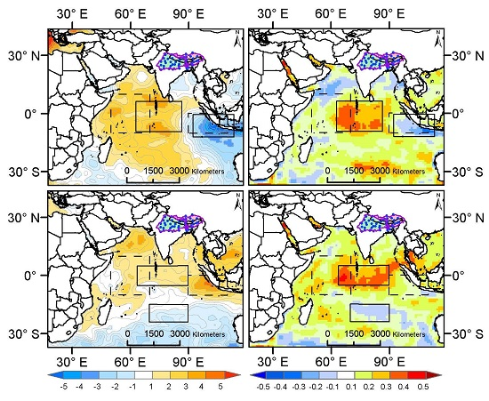
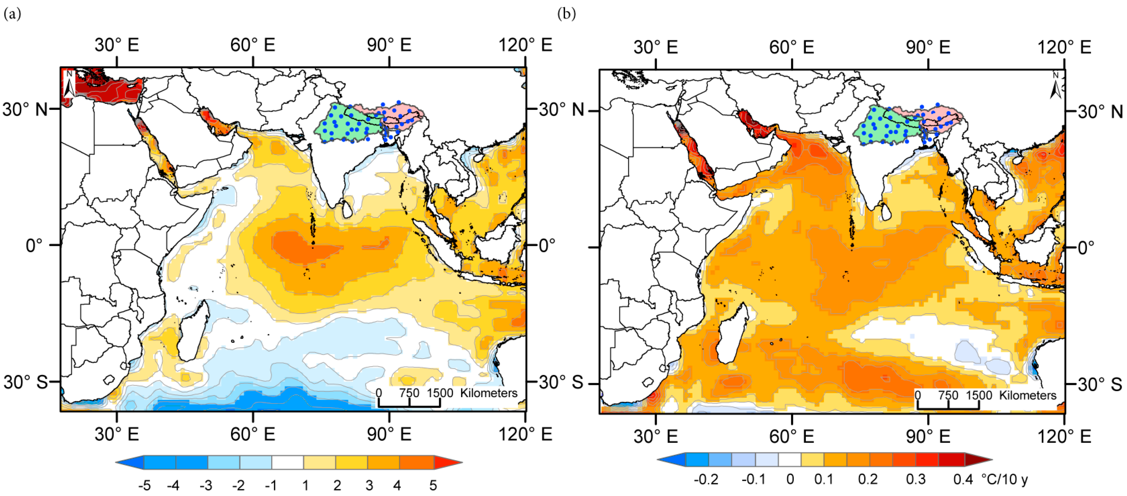
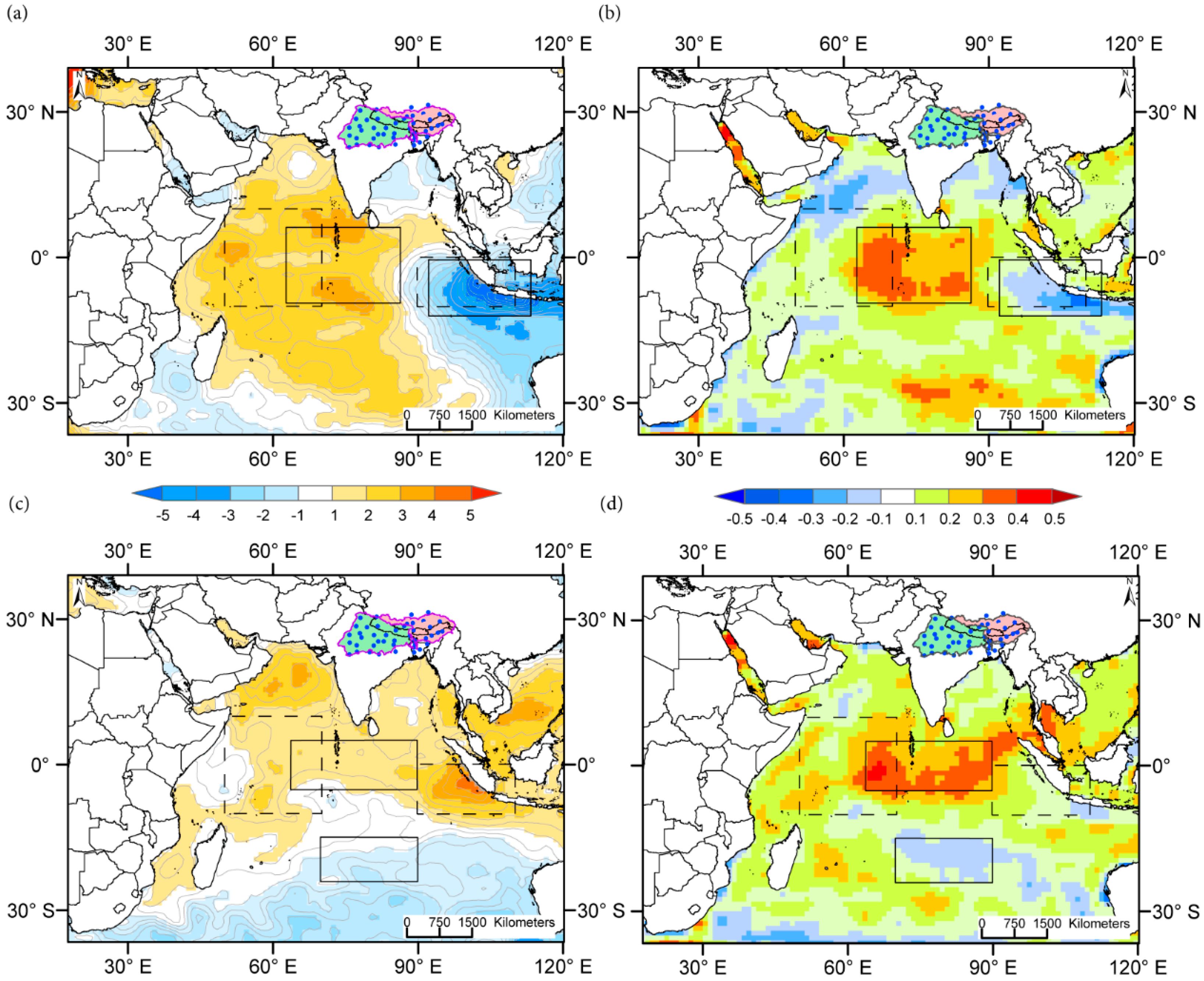
4.1. Patterns of IO SST Spatial Structure

Using EOF analysis of the unfiltered monthly average IO SST anomalies, we find the leading mode (EOF1) differentiates the northern warmer tropical IO from the cooler southern IO (>20°S) and explains 37% of the SST variability during 1982–2010 (Figure 1a and Figure S1a). For this study, IO is defined by the coastal boundaries for the longitudes and north latitude and 20° in the south latitude. Here, we optimize the EOF1 for January–December averages to capture the annual average SST variation pattern in the IO domain. The modes of the EOF depict dominant patterns in the SST variations; however, they do not explain the underlying processes responsible for the variations [41]. Thus, we analyzed the gridded SST rate of change map to explain the observed variation in EOF1. By regressing the gridded SSTs linearly with time [41], we created an SST change map of the IO (Figure 1b) that shows the IO SST increased at a rate between 0.1 °C and 0.4 °C per 10-year during 1982–2010. A nonparametric Mann Kendall trend test (MK-stat 2.8, p = 0.002) also detects a significant increasing trend in the mean IO SST during the study period, which is in agreement with other studies [16,42].

The second leading mode (EOF2) shows a recognizable dipole pattern in the SST variability along the equatorial IO, which accounts for 12.5% of the SST variation (Figure 2a). In Figure 2b, a dipole pattern, similar in structure to EOF2, emerges in the correlation (teleconnection) between grid cells of monthly SST anomalies and the Ganges precipitation. The EOF2 and correlations are optimized for June–November monthly averages when variations in SST are large. The EOF2 identifies the high SST variation sectors (positive and negative), and the correlations between SST and Ganges precipitation illustrates high positive and negative influential sectors for the Ganges precipitation along the west-east direction. Considering the SST variation pattern and the correlations, we propose a new west-east Differential Heating Index (DHI_west-east), computed from the zonal difference SST anomalies from the optimized western and eastern sectors at 63°E–86°E, 6°N–9°S, and 92°E–113°E, equator–12°S (solid-lined boxes in Figure 2a,b). DHI_west-east appears to capture the SST influence on the Ganges precipitation better than DMI_saji (partial correlation $r_{DHIwest-east}=0.41,p<0.0001$ and $r_{NINO3}=-0.40,p<0.0001$ compared to $r_{DMIsaji}=0.30,p<0.0001;r_{NINO3}=-0.35,p<0.0001$). The time series associated with IO EOF2 agrees well with DHI_west-east $r=0.80,p<0.0001$, matching the positive and negative extreme DHI_west-east events in 1994, 1997, 2006 ($>2\sigma$ differential warming over 63°E–86°E, 6°N–9°S region), and 1998 ($>1.5\sigma$ differential warming over 92°E–113°E, equator–12°S region), as shown in Figure S1b.

In the third leading mode (EOF3) also optimized for June through November, we find another 11% of the SST variation is depicted in a distinct recognizable pattern but, unlike the EOF2, the pattern is polarized in the north-south direction (Figure 2c). The correlations between the Brahmaputra precipitation and gridded SST in Figure 2d also shows distinguishable spatial structure where the sector in the central IO is positively correlated to the Brahmaputra precipitation, and the sector in the southern IO is negatively correlated with the same precipitation. Based on the convergence of evidence from these two spatial structures shown in Figure 2c,d, we proposed another new DHI with north-south orientation (DHI_north-south). It is computed from the zonal difference SST anomalies from northern and southern sectors at 61°E–93°E, 5°N–7°S, and 69°E–92°E, 12°S–21°S (solid-lined boxes in Figure 2c,d), and exhibits better correlation than that of DMI_saji with Brahmaputra precipitation (partial correlation $r_{DHInorth-south}=0.59,p<0.0001$ and $r_{NINO3}=-0.20,p<0.009$ compared to $r_{DMIsaji}=0.06,p<0.46;r_{NINO3}=-0.19,p<0.0001$).

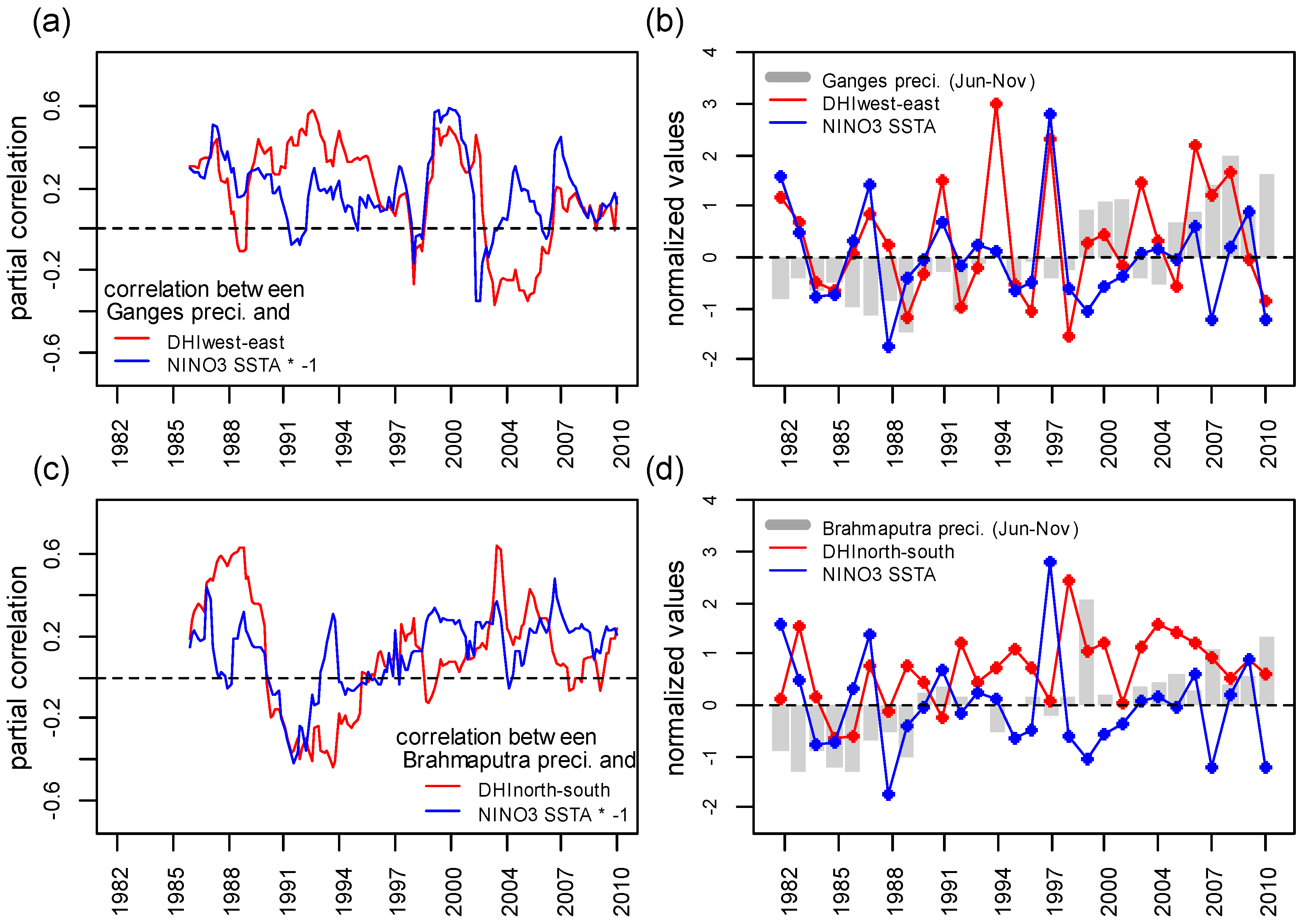
4.2. Interactive Influence of DHI and ENSO on Basin Precipitation

As the influence of the IO dipole and ENSO on precipitation have shown changes over time [13,43], we analyzed moving partial correlation between the basin precipitation and the newly constructed DHIs (DHI_west-east and DHI_north-south), along with those between basin precipitation and ENSO indices to examine the climate modes’ interactive influence during the study period (Figure 3a,c for the Ganges and Brahmaputra, respectively). The moving partial correlation following the method provided in [13] is computed with an interval of 4 years, which is recognized as a typical recurrence interval of the dipole modes [43]. Figure 3b,d shows the time evolution of the complementary influence of these new DHIs and ENSO on precipitation in the Ganges (Figure 3b) and the Brahmaputra (Figure 3d) basins. The correlation coefficient between ENSO index and the Ganges precipitation is about −0.5 in 1987, after which the correlation drops abruptly (Figure 3a). The strong El Niños of 1982 and 1987 (>1.5σ higher SST over NINO3 region, Figure 3b) as well as the moderate El Niños of 1983 and 1986 (about 0.5σ higher SST over NINO3 region, Figure 3b), which were associated with neutral DHI_west-east, dominated the influence on the precipitation (Figure 3b) and resulted in below average precipitation during the 1980s in the Ganges basin. Starting in the late 1980s, the ENSO-precipitation relationship weakened until 1998 (Figure 3a). This sequence agrees with other research findings indicating a weak correlation between ENSO and all-India precipitation [13,44]. Meanwhile, during this period, the influence shifted to DHI_west-east. The strongly positive phases of DHI_west-east during 1991 (>1.5σ differential warming over 63°E–86°E, 6°N–9°S region, Figure 3b) and 1994 (>3.0σ differential warming over 63°E–86°E, 6°N–9°S region, Figure 3b) contributed to a high correlation (>+0.3) between DHI_west-east and the Ganges precipitation during much of the 1990s with close to average precipitation in the Ganges basin. The exceptionally strong El Niño of 1997 (>3.0σ higher SST over NINO3 region, Figure 3b) shifted the influence on precipitation back to ENSO (>−0.5, Figure 3a) until 2000. Although the 1997 El Niño produced below average precipitation, its impact was minimized by the presence of a strong positive DHI_west-east (>2.0σ differential warming over 63°E–86°E, 6°N–9°S region, Figure 3b) in the same year. Prevailing concurrent La Niña during the late 1990s and early 2000s contributed to the high correlation between ENSO and precipitation (Figure 3a). A shift toward the influence of DHI_west-east occurred during the mid-2000s; however, the influence of ENSO was still active during the same time period. While both ENSO-precipitation and DHI_west-east-precipitation relationships were weak, the presence of concurrent strongly positive DHI_west-east in 2006, 2007, and 2008 (>1.0σ differential warming over 63°E–86°E, 6°N–9°S region), coupled with the La Niña of 2007 (<1.0σ lower SST over NINO3 region), produced higher precipitation (>1.5σ higher precipitation) during the latter part of the 2000s in the Ganges basin (Figure 3b).

The correlation coefficient between DHI_north-south and Brahmaputra precipitation was above 0.5 during the latter half of the 1980s (Figure 3c). Precipitation was below average during the 1980s as a result of the El Niño episodes (>1.5σ higher SST over NINO3 region, Figure 3d) in 1982 and 1987. During the first half of the 1990s, the relationships between precipitation and both DHI_north-south and ENSO weakened significantly, and the neutral influence of the climate modes led to average precipitation in the basins. With the help of the exceptional El Niño of 1997 (~3.0σ higher SST over NINO3 region, Figure 3d) followed by La Niña phases, the ENSO again started to dominate the influence on Brahmaputra precipitation during late 1990s and early 2000s. Precipitation was below average in 1997, but in 1999 it was exceptionally high (>2.0σ higher precipitation in the Brahmaputra basin, Figure 3d) from the combined influence of La Niña and positive DHI_north-south (higher differential SST over 61°E–93°E, 5°N–7°S region, Figure 3d). The influence shifted to DHI_north-south when a positive DHI_north-south prevailed during 2003–2006 (>1.0σ differential warming over 61°E–93°E, 5°N–7°S region, Figure 3d). During that period, precipitation in the Brahmaputra basin was above average (>0.5σ precipitation) under neutral phases of ENSO (Figure 3d). The development of a strong La Niña in 2007 and 2010 (<1.0σ cooler SST over NINO3 region) helped the correlation of ENSO with precipitation once again rising for the Brahmaputra basin.

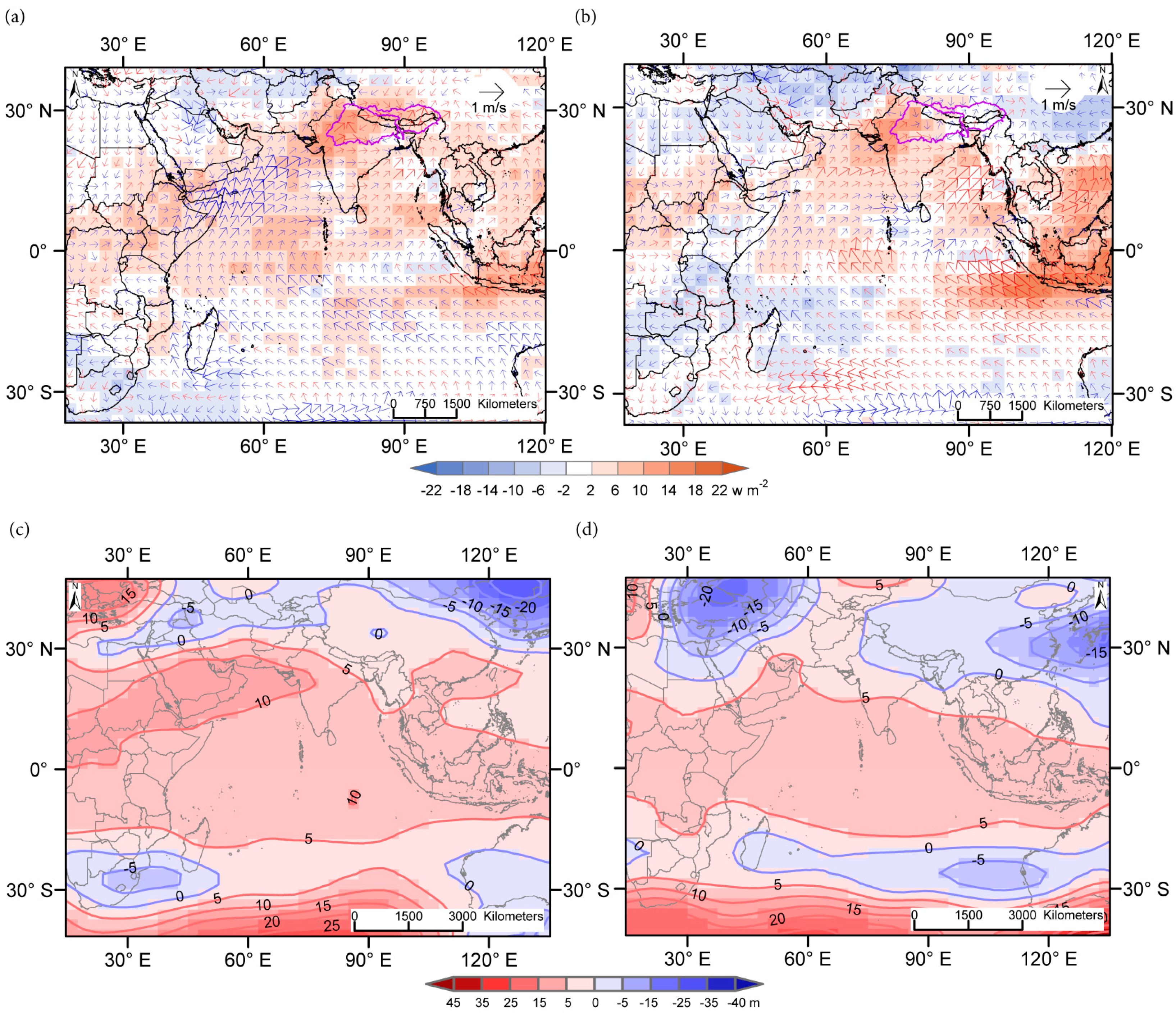
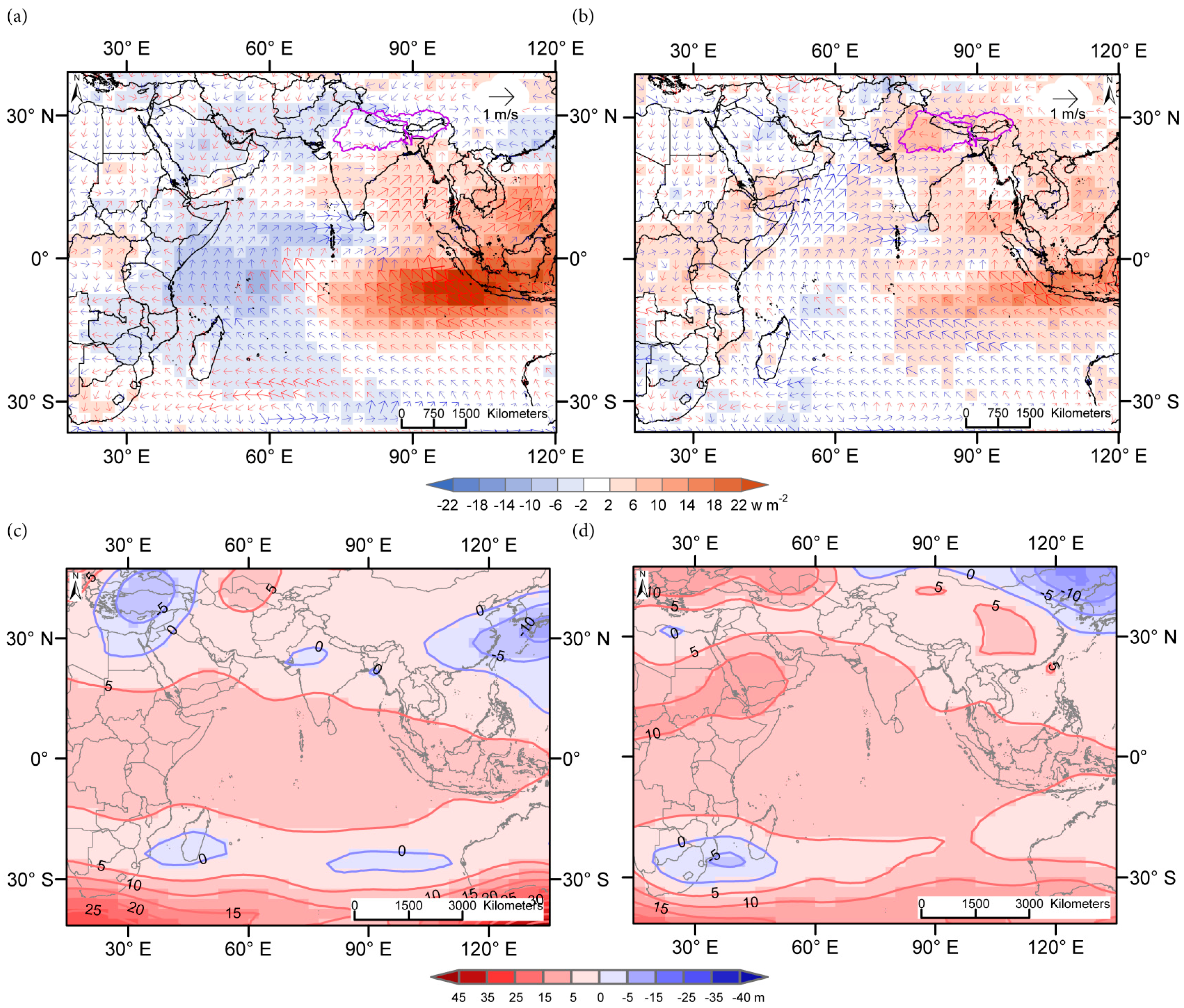
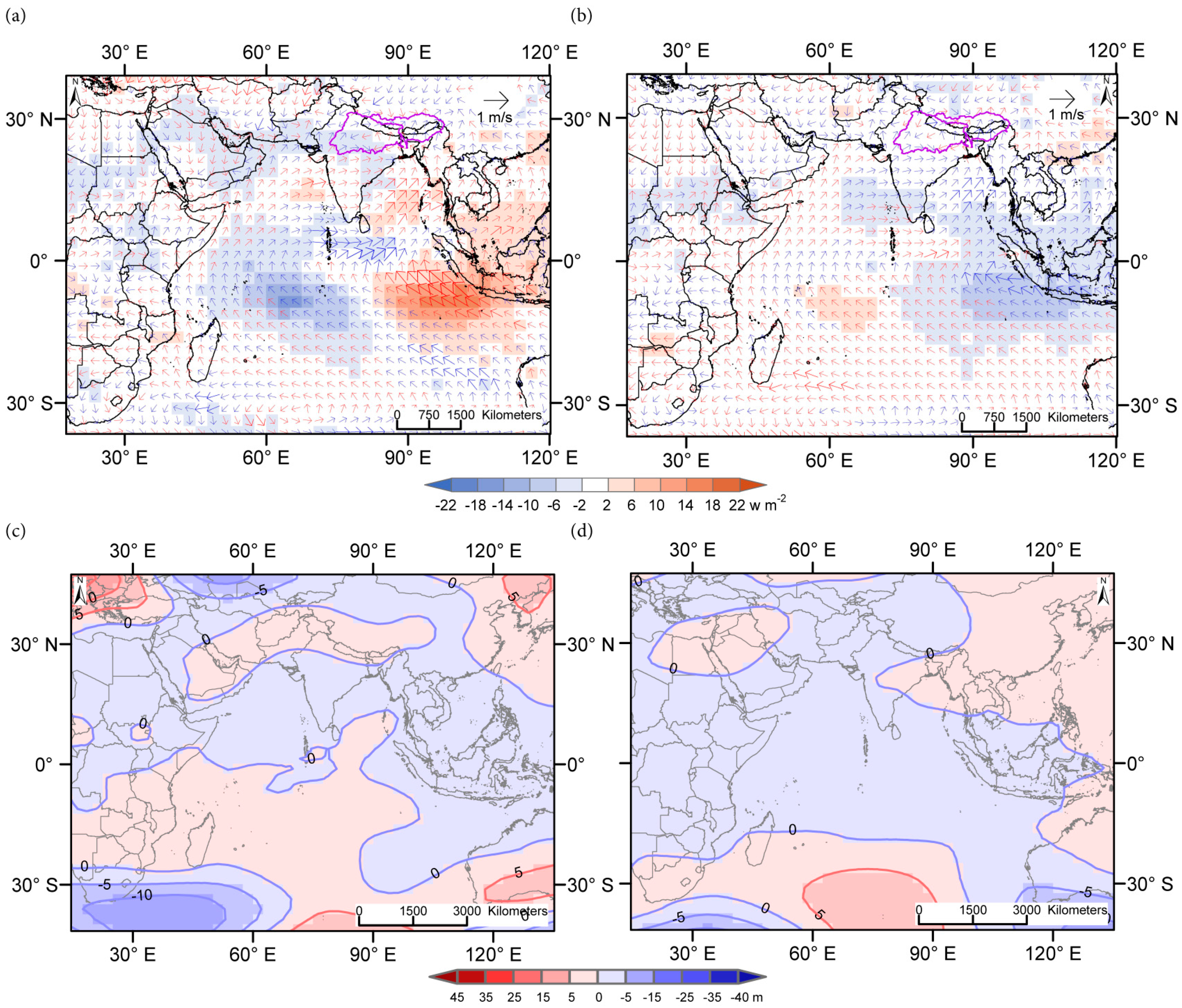
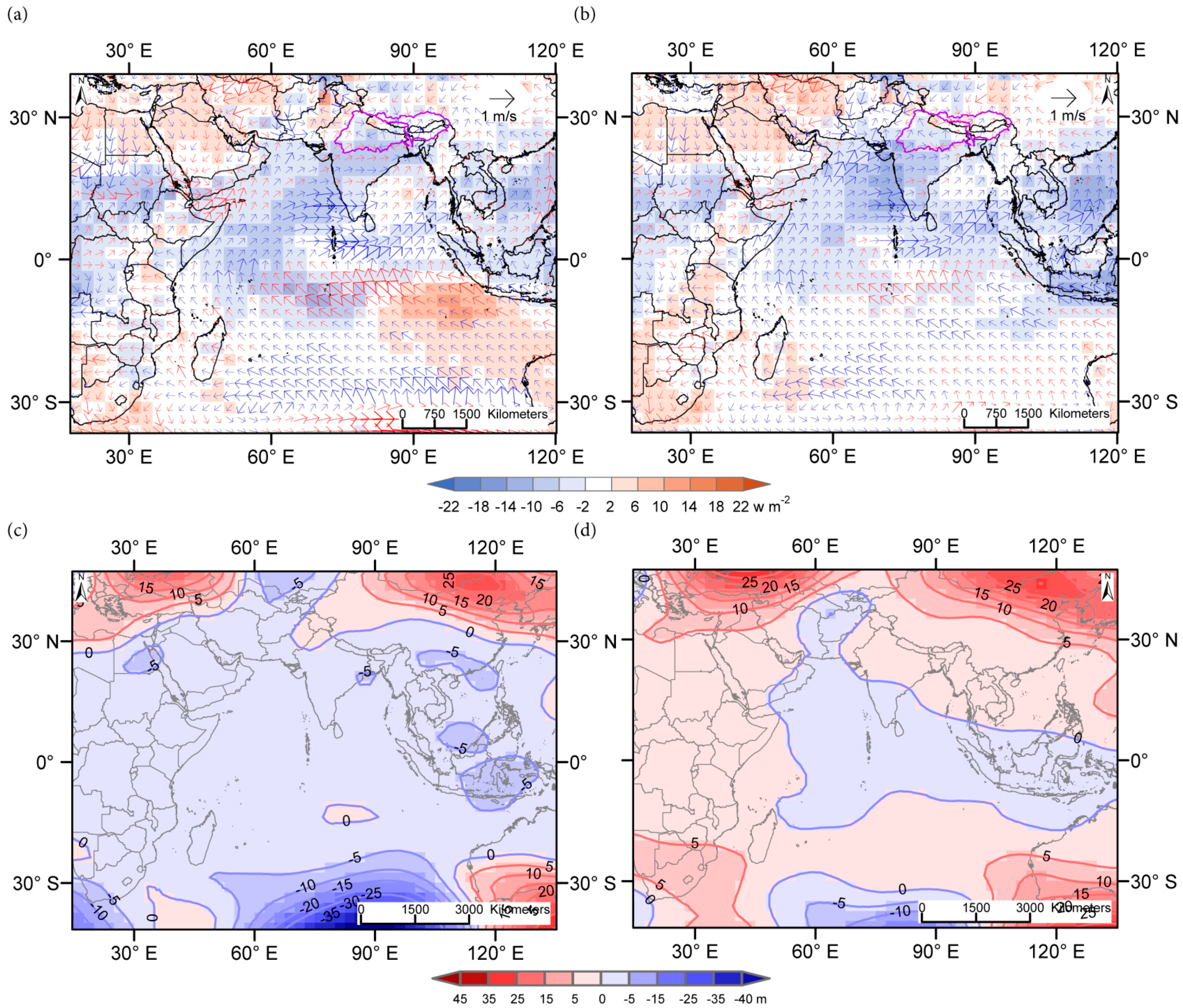
4.3. Wind, OLR, and Geopotential Height Anomalies during Interactive Climate Modes

To further assess the impacts of the interactivity of these climate modes on the basin precipitation, we classify in

Table 1. Classification of years based on impacts of occurrence, co-occurrence, or absence of climate mode (DHI_west-east, ENSO) extremes. Precipitation values are averaged over the July through November period, with the baseline being the observed precipitation during the absence of climate mode extremes (neutral years). In no year was the co-occurrence of El Niño and negative DHI_west-east observed for the Ganges basin during the period 1982–2010 (excluding 2002).

El Niño & Negative DHIwest-east	El Niño& Neutral DHIwest-east	El Niño & Positive DHIwest-east
No years observed	1987, 2009	1982, 1997, 2006
	Avg.: 651 mm, 71% of baseline	Avg.: 866 mm, 94% of baseline
Neutral & Negative DHIwest-east	Neutral	Neutral & Positive DHIwest-east
1989, 1992, 1996, 1998	1983, 1986, 1990, 1993, 1995, 2000, 2001, 2004, 2005	1991, 1994, 2003, 2008
Avg.: 699 mm, 76% of baseline	Baseline = 921 mm	Avg.: 1022 mm, 111% of baseline
La Niña & Negative DHIwest-east	La Niña and Neutral DHIwest-east	La Niña & Positive DHIwest-east
1984, 1985	1988, 2010	1999, 2007
Avg.: 739 mm, 80% of baseline	Avg.: 1035 mm, 112% of baseline	Avg.: 1277 mm, 138% of baseline

and

Table 2. Classification of years based impacts of occurrence, co-occurrence, or absence of climate mode (DHI_north-south, ENSO) extremes. Brahmaputra precipitation values are averaged over the July through November period, with the baseline being the observed precipitation during the absence of climate mode extremes (neutral years). In no year was the co-occurrence of El Niño/neutral and negative DHI_north-south observed for the Brahmaputra basin during the period 1982–2010 (excluding 2002).

El Niño & Negative DHInorth-south	El Niño & Neutral DHInorth-south	El Niño & Positive DHInorth-south
No years observed	1982, 1997	1987, 2006, 2009
	Avg.: 609 mm, 87% of baseline	Avg.: 786 mm, 111% of baseline
Neutral &Negative DHInorth-south	Neutral	Neutral & Positive DHInorth-south
No years observed	1983, 1986, 1990, 1991, 1993, 1994, 1996, 2001, 2008	1989, 1992, 1995, 1998, 2000, 2003, 2004, 2005
	Baseline = 704 mm	Avg.: 799 mm, 113% of baseline
La Niña & Negative DHInorth-south	La Niña & Neutral DHInorth-south	La Niña & Positive DHInorth-south
1984, 1985	1988	1999, 2007, 2010
Avg.: 606 mm, 86% of baseline	Avg.: 620 mm, 88% of baseline	Avg.: 1192 mm, 169% of baseline

the years according to the independent, combined, or neutral influence of the climate modes on the basin precipitation, and analyze the anomalies for precipitation, surface wind velocity, OLR, and geopotential height anomalies. OLR is a measure of the amount of energy emitted to space by the Earth’s surface, oceans, and atmosphere. OLR anomalies are of particular interests because OLR values are often used as a proxy for convection in tropical and subtropical regions since cloud top temperatures (colder is higher) are an indicator of cloud height [45], cloudiness, or cloud cover [46]. While surface wind and OLR state the conditions at surface to near surface, geopotential height anomalies at 500 hPa pressure level state the conditions at upper atmosphere (at variable altitude ~5.5 km). The geopotential height anomalies consist of a positive phase featuring below average geopotential heights, which are also referred to as negative geopotential height anomalies, and a negative phase featuring above average geopotential heights. These phases depict synoptic atmospheric circulation patterns at the mid-troposphere level that correlate well with variabilities in precipitation and temperature [47,48,49]. A positive geopotential height phase compared to other locations at the same latitude indicates the presence of a storm or trough, while the negative phase indicates a ridge associated with quiescent weather. Precipitation under neutral conditions of both ENSO and new DHIs was considered as the baseline. During the studied 28 years, the El Niño impact produced lower precipitation regimes, 71% and 87% of baseline, in the Ganges and Brahmaputra basins, respectively (Table 1 and Table 2); these results are supported by other studies [46,50]. Classification of years in Table 1 and Table 2 for the occurrence, co-occurrence, or absence of climate modes (DHI_west-east, DHI_north-south, El Niño, La Niña) were done based around one standard deviation departure of the climate mode indices from their long-term respective means [51]. During an independent El Niño influence on the Ganges precipitation, the surface wind strengthens along the east coast of Africa, but it weakens over the northern Arabian Sea and Indian sub-continent shown in Figure 4a. The OLR increases anomalously over the same region along with anomalously high (up to 10 m above average) geopotential heights extending up to 30°N (Figure 4c). When El Niño influence persists in the Brahmaputra precipitation, below average wind and positive OLR anomalies prevail over the eastern equatorial IO, but the surface winds increase along with colder cloud tops in the western equatorial IO (Figure 4b). Anomalously high geopotential heights still persist in the equatorial IO, but extend only up to about 20°N (Figure 4d). Beyond 20°N, a wave of cold air mass covers the upper latitudes including much of continental India.

When El Niño co-occurs with positive modes of the new DHIs, the influence of El Nino on precipitation is attenuated. Precipitation increases to 94% and 111% of baseline in the Ganges and Brahmaputra basins, respectively; although it is still below the baseline for the Ganges (Table 1). When positive DHI_west-east (warmer 63°E–86°E, 6°N–9°S region) prevails during an El Niño year, the surface wind increases along with reduced OLR in the western IO and the opposite in the eastern IO. However, the geopotential height anomalies are still positive extending up to 15°N (Figure 5a,c).

When El Niño and positive DHI_north-south (warmer 61°E–93°E, 5°N–7°S region) co-occur, the positive OLR anomalies decrease over the eastern equatorial IO and turns neutral (average convection or cloud cover) over the Arabian Sea and Bay of Bengal along with increased wind (Figure 5b) compared to El Niño conditions (Figure 4b).

Precipitation regime is enhanced during positive phases of the new DHIs in both basins. The Ganges precipitation reaches 111% of baseline and the Brahmaputra precipitation attains 113% of baseline during positive phases of DHI_west-east (warmer 63°E–86°E, 6°N–9°S region) and DHI_north-south (warmer 61°E–93°E, 5°N–7°S region), respectively, when ENSO is neutral. During positive phases of DHI_west-east, the anomalously negative OLR (colder cloud top or higher cloud) along with increased surface winds prevails in the western IO, while positive OLR (warmer cloud top) with reduced surface winds persists in the eastern equatorial IO and the Bay of Bengal forming a dipole pattern (Figure 6a). The condition of the upper atmosphere air mass is mostly average to below average across the region (Figure 6c). When positive DHI_north-south is active, the anomalously low OLR (enhanced convection) accompanied by increased surface winds persists in the eastern equatorial IO and the Bay of Bengal (Figure 6b) and the geopotential height anomalies are average to below average over the region (Figure 6d).

The most favorable conditions for precipitation in both basins are manifested by positive modes of the new DHIs co-occurring with La Niña. Precipitation is observed to increase to 138% and 169% of baseline in the Ganges and Brahmaputra basins, respectively. During the co-occurrences of positive DHI_west-east (warmer 63°E–86°E, 6°N–9°S region) and La Niña, surface wind increases accompanied by strong negative OLR (colder cloud top or enhanced convection) over the western IO, the Arabian Sea, and the Indian subcontinent extending up to 30°N as shown in Figure 7a. Anomalously low geopotential heights prevail in the IO extending up to 30°N with even stronger troughs located in the eastern equatorial IO (Figure 7c). Strong ridges are also noticeable north of the trough at 30°N. The anomaly map of the geopotential height with the influence of La Niña and positive DHI_west-east is observed to be the opposite of the same with the influence of El Niño.

When positive DHI_north-south (warmer 61°E–93°E, 5°N–7°S region) co-occurs with La Niña, the convection enhances with increased surface wind over the Arabian Sea, the Bay of Bengal, and the eastern equtorial IO (Figure 7b). During the combined influence of La Niña and positive DHI_north-south, the 500 hPa geopotential heights are observed to be anomalously low across the eastern equatorial IO followed by two waves of anomalously high geopotential heights beyond 30°N (Figure 7d).

5. Discussions

The observed SST spatial structure from EOF1 (Figure 1a) exhibits shallow gradients in the warmer IO. These shallow gradients have been called “spatially formless” [5,52] and are found to resemble the rate of the mean SST increase map shown in Figure 2b. This increase in mean IO SST captured by EOF1 is in response to El Niño and La Niña in the Pacific [52]. To demonstrate this linkage, we plot and compare time series associated with EOF1 and IO mean SST anomalies. We note that the EOF1 correlates well with mean IO SST anomalies (Figure S1a), which again correlate well with the modes of ENSO ($r=0.61,p<0.0001$ and $r=0.62,p<0.0001$; not shown). We also note that the response of the mean IO SST lags ENSO by about 4 months (not shown). As the proposed two new DHIs show improved correlation with respective basin precipitation for EOF2 and EOF3, what emerges here is strong evidence that the SST differences between the central and eastern IO are influencing precipitation in the Ganges basin, possibly by modulating the Walker circulation [42,50]. Additionally, the precipitation in the Brahmaputra basin is affected by the SST difference between the northern and southern IO, perhaps through modulation of the Hadley circulation [42,50] during the last 28 years. Therefore, the evidence suggests that the differential heating in the IO and ENSO are equally influential for the variabilities in both basins’ precipitation, but they impact the basins’ precipitation differently.

When El Niño is active, the enhanced OLR over the Arabian Sea and Indian-subcontinent indicates warmer cloud tops, which is associated with suppressed convection. During active El Niño, warm air mass also persists in the upper atmosphere associated with the high geopotential heights at 500 hPa pressure level. Below average surface winds associated with suppressed convection, and warm air mass at the upper atmosphere (Figure 4a,c) help to weaken the Walker and Hadley circulations [50], leading to suppressed precipitation in the Ganges basins. For Brahmaputra precipitation, while the warmer air mass over the equatorial IO and suppressed convection over the eastern equatorial IO impacts the Brahmaputra precipitation adversely, the colder air mass and below average OLR beyond 20°N attenuate the impacts (Figure 4b,d). Therefore, like the Ganges, El Niño suppressed precipitation in the Brahmaputra basin but at a lesser magnitude compared to that of the Ganges precipitation. During the co-occurrences of El Niño and positive DHI_west-east the warmer air mass along the equator and suppressed convection in the eastern IO impacts the Walker and Hadley circulations adversely, but the impacts get attenuated by increased convections in the western IO and neutral to colder upper atmosphere air mass beyond 15°N (Figure 5a,c) resulting in more precipitation in the Ganges compared to precipitation under El Niño condition alone. When Brahmaputra precipitation is impacted by co-occurrence of El Niño and positive DHI_north-south, the average convective activities associated with neutral OLR help maintain above average precipitation in the Brahmaputra basin despite anomalously high geopotential heights across the equatorial IO (Figure 5b,d). During the influence of positive DHI_west-east, the dipole pattern of low and high OLR and surface wind in the western and eastern IO help strengthen the Walker circulation, shaping its ascending motion in the west and descending motion in the east over the Bay of Bengal [50]. The subsiding air from the east joins the divergent easterlies in the southern IO and part of it crosses the equator, which helps strengthen the Hadley cell with ascending motion extending up to 30°N [13,50], affecting the Ganges precipitation positively (Table 1, Figure 6a,c). When positive DHI_north-south is active, the combined impacts of low OLR, increased surface winds, and average to low geopotential heights affect Brahmaputra precipitation positively by strengthening the Hadley circulation [50] (Table 2, Figure 6b,d). During co-occurrences of La Niña and positive DHI_west-east, although the cross-equatorial moisture transport diminishes due to anomalously low winds in the southern IO, the Walker and Hadley cells become well developed [50] because of anomalously high wind accompanied by enhanced convection activities, more persistent cloud cover, and a mid-troposphere cold air mass associated with low geopotential height anomalies across the region (Figure 7a,c). As a result, precipitation increases in the Ganges basin (Table 1). For the Brahmaputra, the enhanced convection, increased surface wind, and colder air mass in the upper atmosphere across the Arabian Sea and Bay of Bengal during co-occurrences of La Niña and positive DHI_north-south (Figure 7b,d) favor well-developed Hadley circulation and subsequently Brahmaputra precipitation increases substantially (Table 2).

6. Conclusions

We have demonstrated that two modes of interannual variability of IO SST, which are evident in the anomalies, can be characterized through a west-east and a north-south Differential Heating Index (DHI). The conventional IO dipole index DMI_saji weakly explains the Ganges precipitation variation (partial correlation $r_{DMIsaji}=0.30,p<0.0001$) and does not explain the Brahmaputra precipitation variation (partial correlation $r_{DMIsaji}=0.06,p<0.46$). In contrast, the new DHI_west-east shows improved association with the Ganges precipitation variation (partial correlation $r_{DHIwest-east}=0.41,p<0.0001$), and the new DHI_north-south captures more precipitation variation in the Brahmaputra basin (partial correlation r_{DHInorth-south} = 0.59, p < 0.0001). These newly constructed IO DHIs have been optimized to assess modal influences on the precipitation dynamics in these two major river basins. Although the length of the observational record is relatively brief, the precipitation anomalies are traceable to the interactive impacts of DHI and ENSO. This new perspective on the dynamic role that the IO plays for regional climatic anomalies offers insights about the distribution, variability, and predictability of precipitation in these major South Asian river basins that can be used for climate change impact assessment and natural hazards forecasting as well as for analysis and contextualization of land cover and land use change.

References

1. Lindzen, R.S.; Nigam, S. On the role of sea surface temperature gradients in forcing low-level winds and convergence in the tropics. J. Atmos. Sci. 1987, 44, 2418–2435. [Google Scholar] [CrossRef]
2. Annamalai, H.; Liu, P.; Xie, S.P. Southwest Indian Ocean SST variability: Its local effect and remote influence on Asian monsoons. J. Clim. 2005, 18, 4150–4167. [Google Scholar] [CrossRef]
3. Cherchi, A.; Gualdi, S.; Behera, S.; Luo, J.J.; Masson, S.; Yamagata, T.; Navarra, A. The influence of tropical Indian Ocean SST on the Indian summer monsoon. J. Clim. 2007, 20, 3083–3105. [Google Scholar] [CrossRef]
4. Van Loon, H.; Meehl, G.A. The Indian summer monsoon during peaks in the 11 years sunspot cycle. Geophys. Res. Lett. 2012, 39, L13701. [Google Scholar] [CrossRef]
5. Saji, N.H.; Goswami, B.N.; Vinayachandran, P.N.; Yamagata, T. A dipole mode in the tropical Indian Ocean. Nature 1999, 401, 360–363. [Google Scholar] [CrossRef] [PubMed]
6. Bjerknes, J. Atmospheric teleconnections from the equatorial Pacific. Mon. Weather Rev. 1969, 97, 163–172. [Google Scholar] [CrossRef]
7. Webster, P.J.; Moore, A.M.; Loschnigg, J.P.; Leben, R.R. Coupled ocean-atmosphere dynamics in the Indian Ocean during 1997–1998. Nature 1999, 401, 356–360. [Google Scholar] [CrossRef] [PubMed]
8. Conway, D.; Hanson, C.E.; Doherty, R.; Persechino, A. GCM simulations of the Indian Ocean dipole influence on east african rainfall: Present and future. Geophys. Res. Lett. 2007, 34, L03705. [Google Scholar] [CrossRef]
9. Reason, C.J.C. Subtropical Indian Ocean SST dipole events and southern african rainfall. Geophys. Res. Lett. 2001, 28, 2225–2227. [Google Scholar] [CrossRef]
10. Abram, N.J.; Gagan, M.K.; McCulloch, M.T.; Chappell, J.; Hantoro, W.S. Coral reef death during the 1997 Indian Ocean dipole linked to indonesian wildfires. Science 2003, 301, 952–955. [Google Scholar] [CrossRef] [PubMed]
11. Zubair, L.; Rao, S.A.; Yamagata, T. Modulation of Sri Lankan Maha rainfall by the Indian Ocean dipole. Geophys. Res. Lett. 2003, 30, 1063. [Google Scholar] [CrossRef]
12. Ummenhofer, C.C.; Gupta, A.S.; Briggs, P.R.; England, M.H.; McIntosh, P.C.; Meyers, G.A.; Pook, M.J.; Raupach, M.R.; Risbey, J.S. Indian and Pacific Ocean influences on southeast Australian drought and soil moisture. J. Clim. 2011, 24, 1313–1336. [Google Scholar] [CrossRef]
13. Ashok, K.; Guan, Z.; Yamagata, T. Impact of the Indian Ocean dipole on the relationship between the Indian monsoon rainfall and ENSO. Geophys. Res. Lett. 2001, 28, 4499–4502. [Google Scholar] [CrossRef]
14. Ashok, K.; Saji, N.H. On the impacts of ENSO and Indian Ocean dipole events on sub-regional Indian summer monsoon rainfall. Nat. Hazards 2007, 42, 273–285. [Google Scholar] [CrossRef]
15. Pervez, M.S.; Henebry, G.M. Spatial and seasonal responses of precipitation in the ganges and brahmaputra river basins to ENSO and Indian Ocean dipole modes: Implications for flooding and drought. Nat. Hazards Earth Syst. Sci. 2015, 15, 147–162. [Google Scholar] [CrossRef]
16. Stocker, T.; Dahe, Q.; Plattner, G.; Alexander, L.; Allen, S.; Bindoff, N.; Breon, F.; Church, J.; Cubasch, U.; Emori, S.; et al. Climate Change 2013: The Physical Science Basis; Working Group I Contribution to the IPCC Fifth Assessment Report; Intergovernmental Panel on Climate Change: Stockholm, Sweden, 2013. [Google Scholar]
17. Chowdhury, M.; Ward, N. Hydro-meteorological variability in the greater ganges–brahmaputra–meghna basins. Int. J. Climatol. 2004, 24, 1495–1508. [Google Scholar] [CrossRef]
18. Pervez, M.S.; Henebry, G.M. Projections of the ganges–brahmaputra precipitation—Downscaled from gcm predictors. J. Hydrol. 2014, 517, 120–134. [Google Scholar] [CrossRef]
19. The World Bank South Asian Water Initiative. The Ganges Strategic Basin Assessment: A Discussion of Regional Opportunities and Risks; 67668-SAS; The World Bank: Washington, DC, USA, 2014. [Google Scholar]
20. Rasul, G. Water for growth and development in the ganges, brahmaputra, and meghna basins: An economic perspective. Int. J. River Basin Manag. 2015, 13, 387–400. [Google Scholar] [CrossRef]
21. Alexandratos, N.; Bruinsma, J. World Agriculture Towards 2030/2050: The 2012 Revision; ESA Working Paper; Food and Agriculture Organization of the United Nations: Rome, Italy, 2012. [Google Scholar]
22. Thenkabail, P.S.; Schull, M.; Turral, H. Ganges and indus river basin land use/land cover (LULC) and irrigated area mapping using continuous streams of MODIS data. Remote Sens. Environ. 2005, 95, 317–341. [Google Scholar] [CrossRef]
23. Ghosh, S.; Vittal, H.; Sharma, T.; Karmakar, S.; Kasiviswanathan, K.; Dhanesh, Y.; Sudheer, K.; Gunthe, S. Indian summer monsoon rainfall: Implications of contrasting trends in the spatial variability of means and extremes. PLoS ONE 2016, 11, e0158670. [Google Scholar] [CrossRef] [PubMed]
24. Immerzeel, W.W. Historical trends and future predictions of climate variability in the Brahmaputra basin. Int. J. Climatol. 2008, 28, 243–254. [Google Scholar] [CrossRef]
25. Mirza, M.Q. Climate change, flooding in South Asia and implications. Reg. Environ. Chang. 2011, 11, 95–107. [Google Scholar] [CrossRef]
26. Jian, J.; Webster, P.J.; Hoyos, C.D. Large-scale controls on ganges and brahmaputra river discharge on intraseasonal and seasonal time-scales. Q. J. R. Meteorol. Soc. 2009, 135, 353–370. [Google Scholar] [CrossRef]
27. Reynolds, R.W.; Rayner, N.A.; Smith, T.M.; Stokes, D.C.; Wang, W. An improved in situ and satellite SST analysis for climate. J. Clim. 2002, 15, 1609–1625. [Google Scholar] [CrossRef]
28. Liebmann, B.; Smith, C.A. Description of a complete (interpolated) outgoing longwave radiation dataset. Bull. Am. Meteorol. Soc. 1996, 77, 1275–1277. [Google Scholar]
29. Kalnay, E.; Kanamitsu, M.; Kistler, R.; Collins, W.; Deaven, D.; Gandin, L.; Iredell, M.; Saha, S.; White, G.; Woollen, J.; et al. The NCEP/NCAR 40-year reanalysis project. Bull. Am. Meteorol. Soc. 1996, 77, 437–471. [Google Scholar] [CrossRef]
30. National Oceanic and Atmospheric Administration, Oceanic and Atmospheric Research/Earth System Research Laboratory Physical Science Division, Climate Research and Reanalysis Datasets. Available online: http://www.esrl.noaa.gov/psd/ (accessed on 6 October 2012).
31. National Climatic Data Center. Global Surface Summary of the Day—GSOD, Version 7. 2001. Available online: ftp://ftp.ncdc.noaa.gov/pub/data/gsod (accessed on 5 January 2012). [Google Scholar]
32. Pervez, M.S.; Henebry, G.M. Assessing the impacts of climate and land use and land cover change on the freshwater availability in the Brahmaputra river basin. J. Hydrol. Reg Stud. 2015, 3, 285–311. [Google Scholar] [CrossRef]
33. Qian, Y.; Gong, D.; Leung, R. Light rain events change over North America, Europe, and Asia for 1973–2009. Atmos. Sci. Lett. 2010, 11, 301–306. [Google Scholar] [CrossRef]
34. Räsänen, T.A.; Kummu, M. Spatiotemporal influences of ENSO on precipitation and flood pulse in the Mekong River Basin. J. Hydrol. 2013, 476, 154–168. [Google Scholar] [CrossRef]
35. Siddique-E-Akbor, A.H.M.; Hossain, F.; Sikder, S.; Shum, C.K.; Tseng, S.; Yi, Y.; Turk, F.J.; Limaye, A. Satellite precipitation data–driven hydrological modeling for water resources management in the Ganges, Brahmaputra, and Meghna basins. Earth Interact. 2014, 18, 1–25. [Google Scholar] [CrossRef]
36. Joyce, R.J.; Janowiak, J.E.; Arkin, P.A.; Xie, P. Cmorph: A method that produces global precipitation estimates from passive microwave and infrared data at high spatial and temporal resolution. J. Hydrometeorol. 2004, 5, 487–503. [Google Scholar] [CrossRef]
37. Huffman, G.J.; Adler, R.F.; Bolvin, D.T.; Nelkin, E.J. The trmm multi-satellite precipitation analysis (TMPA). In Satellite Rainfall Applications for Surface Hydrology; Springer: Dordrecht, The Netherlands, 2010; pp. 3–22. [Google Scholar]
38. Fisher, R.A. Statistical Methods for Research Workers, 5th ed.; Oliver and Boyd: London, UK, 1925. [Google Scholar]
39. Kendall, M.G. Rank Correlation Methods, 5th ed.; Griffin: London, UK, 1990. [Google Scholar]
40. Mann, H.B. Nonparametric tests against trend. Econometrica 1945, 13, 245–259. [Google Scholar] [CrossRef]
41. Dommenget, D. An objective analysis of the observed spatial structure of the tropical Indian Ocean SST variability. Clim. Dyn. 2011, 36, 2129–2145. [Google Scholar] [CrossRef]
42. Han, W.; Meehl, G.A.; Rajagopalan, B.; Fasullo, J.T.; Hu, A.; Lin, J.; Large, W.G.; Wang, J.W.; Quan, X.W.; Trenary, L.L.; et al. Patterns of Indian Ocean sea-level change in a warming climate. Nat. Geosci. 2010, 3, 546–550. [Google Scholar] [CrossRef]
43. Abram, N.J.; Gagan, M.K.; Cole, J.E.; Hantoro, W.S.; Mudelsee, M. Recent intensification of tropical climate variability in the Indian Ocean. Nat. Geosci. 2008, 1, 849–853. [Google Scholar] [CrossRef]
44. Trenberth, K.E.; Caron, J.M. The southern oscillation revisited: Sea level pressures, surface temperatures, and precipitation. J. Clim. 2000, 13, 4358–4365. [Google Scholar] [CrossRef]
45. National Center for Atmospheric Research Staff (Ed.) The Climate Data Guide: Outgoing Longwave Radiation (OLR): AVHRR. Available online: https://climatedataguide.ucar.edu/climate-data/outgoing-longwave-radiation-olr-avhrr (accessed on 6 October 2015).
46. Ardanuy, P.E.; Kyle, H.L. El Niño and outgoing longwave radiation: Observations from Nimbus-7 ERB. Mon. Weather Rev. 1986, 114, 415–433. [Google Scholar] [CrossRef]
47. Tymvios, F.; Savvidou, K.; Michaelides, S. Association of geopotential height patterns with heavy rainfall events in Cyprus. Adv. Geosci. 2010, 23, 73–78. [Google Scholar] [CrossRef] [Green Version]
48. Xoplaki, E.; Luterbacher, J.; Burkard, R.; Patrikas, I.; Maheras, P. Connection between the large-scale 500 hPa geopotential height fields and precipitation over greece during wintertime. Clim. Res. 2000, 14, 129–146. [Google Scholar] [CrossRef]
49. Kożuchowski, K.; Wibig, J.; Maheras, P. Connections between air temperature and precipitation and the geopotential height of the 500 hPa level in a meridional cross-section in Europe. Int. J. Climatol. 1992, 12, 343–352. [Google Scholar] [CrossRef]
50. Ashok, K.; Guan, Z.; Saji, N.H.; Yamagata, T. Individual and combined influences of ENSO and the Indian Ocean dipole on the Indian summer monsoon. J. Clim. 2004, 17, 3141–3155. [Google Scholar] [CrossRef]
51. Meyers, G.; McIntosh, P.; Pigot, L.; Pook, M. The years of el niño, la niña and interactions with the tropical Indian Ocean. J. Clim. 2007, 20, 2872–2880. [Google Scholar] [CrossRef]
52. Wallace, J.M.; Rasmusson, E.M.; Mitchell, T.P.; Kousky, V.E.; Sarachik, E.S.; von Storch, H. On the structure and evolution of ENSO-related climate variability in the tropical Pacific: Lessons from TOGA. J. Geophys. Res. 1998, 103, 14241–14259. [Google Scholar] [CrossRef]
53. Pervez, M.S.; Henebry, G.M. Differential Heating in the Indian Ocean Differentially Modulates Precipitation in the Ganges and Brahmaputra Basins. U.S. Geological Survey Data Release, 2016. Available online: https://dx.doi.org/10.5066/F77P8WH6 (accessed on 25 October 2016). [Google Scholar]
Figure 1. (a) Leading mode of the empirical orthogonal function (EOF1) of January through December Sea Surface Temperature (SST) anomaly during 1982 to 2010, showing the dipole in SST with the divergence occurring around 20°S; (b) Spatial pattern of the rate of change (°C/10 year) in SST in the Indian Ocean. The rate of change in SST was computed by linearly regressing time series SST anomalies at each grid cell. Light green and pink polygons indicate the Ganges and Brahmaputra basins, respectively. Blue dots are GSOD precipitation station locations.
Remotesensing 08 00901 g001
Figure 2. (a) Second mode of the empirical orthogonal function (EOF2) of the SST anomalies showing a dipole pattern along the west-east direction in the Indian Ocean; (b) Spatial pattern of the correlations between each grid cell of the SST anomaly and the Ganges precipitation; (c) Third mode of the empirical orthogonal function (EOF3) of the SST anomalies showing the north-south dipole pattern; (d) Spatial pattern of the correlations between each grid cell of the SST anomaly and the Brahmaputra precipitation. The EOF and correlation map are optimized for June-November averages. Solid-lined boxes in (a,b) are the sectors used to compute the new west-east Differential Heating Index (DHIwest-east); and in (c,d) are the sectors to compute the new north-south DHI (DHInorth-south). Dash-lined boxes are the original sectors defined by [5] DMIsaji. Light green and pink polygons indicate the locations of the Ganges and Brahmaputra basins, respectively. Blue dots are the GSOD precipitation station locations.
Remotesensing 08 00901 g002
Figure 3. (a) Four-year moving partial correlations between Ganges precipitation (June–November) and DHIwest-east (red line), and Ganges precipitation and NINO3 SST (blue line; to be multiplied by −1); (b) Ganges precipitation (June–November) anomalies (gray bars) with values of DHIwest-east (red line with filled circles) and NINO3 SST (blue line with filled circles); (c) Four-year moving partial correlations between Brahmaputra precipitation (June–November) and DHInorth-south (red line), and Brahmaputra precipitation and NINO3 SST (blue line; to be multiplied by −1); (d) Brahmaputra precipitation (June–November) anomalies (gray bars) with values of DHInorth-south (red line with filled circles) and NINO3 SST (blue line with filled circles).
Remotesensing 08 00901 g003
Figure 4. Average anomalies of outgoing longwave radiation (OLR) and wind for El Niño years (a) From Table 1 (b) From Table 2; and average anomalies of 500 hPa geopotential heights with contours for El Niño years (c) From Table 1 and (d) From Table 2. OLR anomalies are for June-November relative to the 1982–2010 average, and near surface winds and geopotential height anomalies are for June-September relative to the 1981–2010 average, respectively. Red arrows are decreased wind velocities and blue arrows are increased wind velocities. Arrow length indicates the magnitude of the velocity and arrow bearing indicates wind direction.
Remotesensing 08 00901 g004
Figure 5. Average anomalies of outgoing longwave radiation (OLR) and wind for El Niño and positive DHIs years (a) From Table 1 (b) From Table 2; and average anomalies of 500 hPa geopotential heights with contours for El Niño and positive DHIs years (c) From Table 1 and (d) From Table 2. OLR anomalies are for June–November relative to the 1982–2010 average, and near surface winds and geopotential height anomalies are for June-September relative to the 1981–2010 average, respectively. Red arrows are decreased wind velocities and blue arrows are increased wind velocities. Arrow length indicates the magnitude of the velocity and arrow bearing indicates wind direction.
Remotesensing 08 00901 g005
Figure 6. Average anomalies of outgoing longwave radiation (OLR) and wind for (a) Positive DHIwest-east years from Table 1 (b) Positive DHInorth-south years from Table 2; and average anomalies of 500 hPa geopotential heights with contours for (c) Positive DHIwest-east years from Table 1 and (d) Positive DHInorth-south years from Table 2. OLR anomalies are for June–November relative to the 1982–2010 average, and near surface winds and geopotential height anomalies are for June–September relative to the 1981–2010 average, respectively. Red arrows are decreased wind velocities and blue arrows are increased wind velocities. Arrow length indicates the magnitude of the velocity and arrow bearing indicates wind direction.
Remotesensing 08 00901 g006
Figure 7. Average anomalies of outgoing longwave radiation (OLR) and wind for La Niña and positive DHIs years (a) From Table 1 (b) From Table 2; and average anomalies of 500 hPa geopotential heights with contours for La Niña and positive DHIs years (c) From Table 1 and (d) From Table 2. OLR anomalies are for June–November relative to the 1982–2010 average, and near surface winds and geopotential height anomalies are for June–September relative to the 1981–2010 average, respectively. Red arrows are decreased wind velocities and blue arrows are increased wind velocities. Arrow length indicates the magnitude of the velocity and arrow bearing indicates wind direction.
Remotesensing 08 00901 g007